Vegetation Dynamics of Sub-Mediterranean Low-Mountain Landscapes under Climate Change (on the Example of Southeastern Crimea)

Abstract

In the context of a changing environment, understanding the interaction between vegetation and climate is crucial for assessing, predicting, and adapting to future changes in different vegetation types. Vegetation exhibits high sensitivity to external environmental factors, making this understanding particularly significant. This study utilizes geospatial analysis techniques, such as geographic information systems, to investigate vegetation dynamics based on remote sensing data and climatic variables, including annual air temperature, annual precipitation, and annual solar radiation. The research methodology encompasses data collection, processing, and analysis, incorporating multispectral imagery and multilayered maps of various parameters. The calculation of the normalized difference vegetation index serves to evaluate changes in vegetation cover, identify areas experiencing variations in green biomass, and establish strategies for the future development of different vegetation types. During the period from 2001 to 2022, the average normalized difference vegetation index value in the Southeastern Crimea region amounted to 0.443. The highest average values were recorded in the year 2006, reaching a magnitude of 0.469. Conversely, the lowest values were observed in the years 2001–2002, constituting 0.397. It has been ascertained that an overarching positive trend in the evolution of NDVI values from 2001 to 2022 is apparent, thus implying a notable augmentation in vegetative biomass. However, adversarial trends manifest in discrete locales adjacent to the cities of Sudak and Feodosia, along with the coastal stretches of the Black Sea. Correlation analysis is employed to establish relationships between vegetation changes and climatic indicators. The findings contribute to our understanding of the vulnerability of various vegetation types and ecosystems in the Southeastern Crimea region. The obtained data provide valuable insights for the development of sustainable vegetation resource management strategies and climate change adaptation in the region.

1. Introduction

Vegetation change is considered a key indicator of ecosystem response to environmental factors and conditions [1,2]. Global vegetation change has become a pressing issue in recent years, posing a significant threat [3,4]. Consequently, all countries are actively involved in addressing the drastic reduction of global vegetation cover, as evidenced by the inclusion of this topic in various regulatory documents worldwide [5,6]. Climate factors exert a profound influence on vegetation change [7,8,9,10], while endogenous catastrophic processes, such as earthquakes [11], volcanic eruptions [12], fires [13], erosion-induced loss of topsoil fertility [14,15], floods [16], adverse atmospheric phenomena (e.g., hurricanes, typhoons) [17], and plant diseases caused by fungi, lichens, insects, and other agents [18,19], further contribute to the transformation of vegetation. Moreover, anthropogenic activities, encompassing both complex processes and intentional clearing of vegetation for various purposes [20,21,22], significantly impact vegetation change. Deforestation is particularly acute in large timber-rich countries such as Brazil, Canada, China, Russia, and others. Various approaches are employed to assess vegetation change, including computer modeling, remote sensing methods [23,24,25], changes in land cover composition [26,27,28], alterations in vegetation index characteristics [29,30,31], and the utilization of multispectral satellite imagery for classification purposes [32,33].

Li et al. [34] point out that traditional vegetation dynamics monitoring based on field-sampled data has limitations due to the intricate data collection process, which presents challenges in analyzing long-term changes in vegetation. Consequently, the application of remote sensing methods addresses many challenges when studying vegetation dynamics. In recent years, the use of remote sensing data has enabled the near real-time monitoring of vegetation change, including its qualitative characteristics. The analysis of NDVI dynamics has gained prominence as a widely employed method for assessing vegetation change [30,34,35]. This can be attributed to the simplicity of NDVI calculation and the availability of extensive archives of high-resolution multispectral satellite imagery, such as MODIS, Landsat, Sentinel, and others. Traditionally, NDVI has found practical applications in agriculture [36] for crop condition analysis and the calculation of norms for various land improvement operations. NDVI has been actively applied in recent years to evaluate vegetation change in diverse regions worldwide, including China [37,38,39,40], India [41,42], the United States [43], Russia [41], Bangladesh [28], Argentina [35], Iran [44], Pakistan [31], among others. Gandhi et al. [30] demonstrated the potential of employing NDVI in analyzing vegetation change in the Vellore District, India. They found that forest or shrub land and barren land cover types decreased by approximately 6% and 23%, respectively, from 2001 to 2006. In contrast, agricultural land, built-up areas, and water areas increased by approximately 19%, 4%, and 7%, respectively. Jiang et al. [38], utilizing NDVI calculations, revealed a significant increase in vegetation NDVI in Tibet from 2001 to 2020, with the annual mean NDVI fluctuating between 0.31 and 0.34. Han et al. [37] demonstrated that the NDVI values in Anhui Province ranged between 0.5 and 0.58, with a multi-year annual mean of 0.55. Vegetation cover in Anhui Province gradually improved from 2001 to 2019. Johnson et al. [43] assessed crop productivity in the United States using MODIS NDVI.

It Is essential to recognize that forest landscapes hold significant value within the spectrum of vegetation cover due to their crucial contributions, as highlighted by numerous researchers [45,46,47]. Forests play a vital role in carbon sequestration, exhibiting the highest potential in this regard [48]. They also function as complex ecosystems that influence global substance and energy transformation cycles [49,50], while providing recreational benefits [51]. Among the most vulnerable and susceptible ecosystems are the forests of the Amazon [52,53], Equatorial Africa [54,55], Vietnam [56], and Siberia [57]. Additionally, forests situated at the boundaries of their natural distribution range, subject to negative impacts from both natural and anthropogenic factors, warrant special attention. However, the study of forest landscape functioning often receives insufficient attention.

The Crimean Peninsula, particularly Southeastern Crimea, represents a typical region characterized by vulnerable forest landscapes. Moreover, Southeastern Crimea marks the northern limit of downy oak forests [58]. In addition to forests, the region encompasses a limited number of steppe landscapes, which also respond to climate change.

This study aims to: (1) assess changes in NDVI values within different vegetation communities in Southeastern Crimea from 2001 to 2022; (2) analyze climatic changes in Southeastern Crimea during the same period; (3) establish relationships between climatic changes and vegetation dynamics in Southeastern Crimea from 2001 to 2022; and (4) evaluate trends in vegetation change in Southeastern Crimea from 2001 to 2022.

Section 1 addresses foundational theoretical inquiries concerning the feasibility of investigating vegetation dynamics through the application of the normalized difference vegetation index (NDVI) in conjunction with geoinformatics methodologies. Elaborate scrutiny is directed towards discerning the multifarious factors that exert potential influence upon the alterations within the vegetative canopy. Of particular emphasis is the intricate topic of global forest dynamics and transformation. The inaugural section endeavors to posit the proposition that the assimilation of the NDVI and the employment of remote sensing techniques, including the dissection of satellite-derived imagery and the computation of pertinent vegetation indices, confer the analytical capacity to evaluate the intricate trajectory of vegetation dynamics, encompassing sylvan ecosystems, within the expanse of the delimited study area. Section 2, elucidates the geographical parameters of the research locale, encapsulating its physiogeographic attributes and the botanical composition indigenous to the study domain. Concomitantly, it expounds upon the research methodology grounded in the exploitation of spatiotemporal variations intrinsic to the NDVI. This methodological framework encompasses the computation of trend analyses, coefficient of variation assessments, the application of the Hurst index, and the discernment of climatic influencers shaping vegetational metamorphosis. Within Section 3, a compendium of cartographic representations and graphical depictions, conceived through the implementation of the methodology outlined in Section 2, is presented. Section 4 provides a comprehensive evaluation of the obtained results, including a detailed exploration of their implications and significance. Additionally, this section outlines the inherent limitations that have constrained the scope and applicability of the conducted research. Section 5 encapsulates the definitive postulates derived from the research endeavor. Furthermore, it undertakes a discourse on the potential trajectories for future investigations in this domain.

2. Materials and Methods

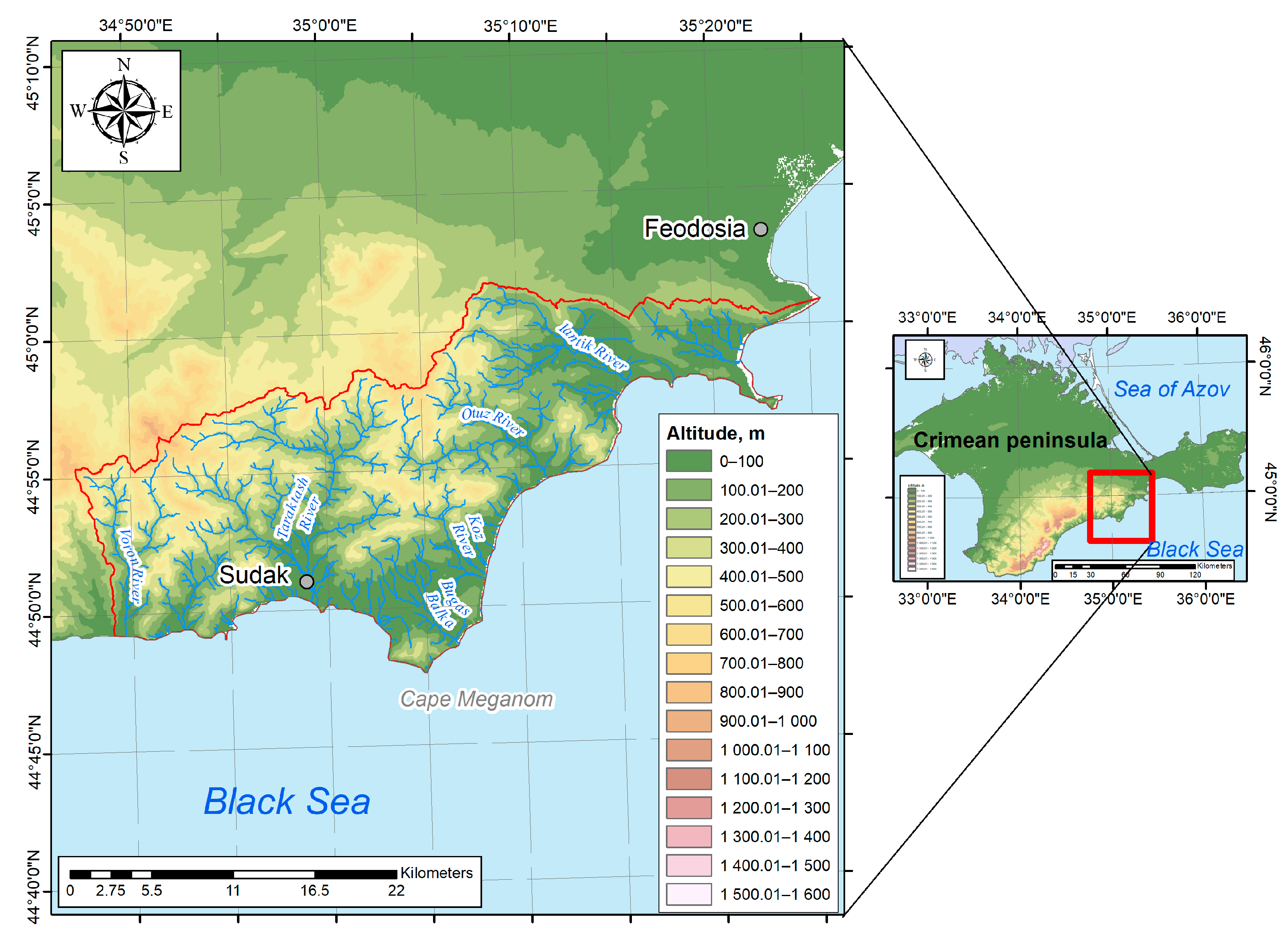
2.1. Study Area

Southeastern Crimea is situated in Eastern Europe, in the southeastern part of the Crimean Peninsula (Figure 1). Its geographical coordinates range from 34°45–35°25′ E and 44°45–44°55′ N. The area of Southeastern Crimea is approximately 568 square kilometers. The boundary of Southeastern Crimea is defined according to [59]. The region is characterized by a complex and rugged terrain, with limited surface water resources. A detailed geographic description of the study area is provided in [58]. The territory of Southeastern Crimea is characterized by Mediterranean climatic features. The average annual air temperature within the Southeastern Crimea area, which varies from the northwest to the southeast, ranges from +9° to +13°. Southeastern Crimea experiences between 100 and 300 mm of precipitation during the winter period. The precipitation field decreases from west to east, with the greatest amount falling in the northwestern part of the study area. In summer, 80 to 160 mm of precipitation falls over the territory of Southeastern Crimea, with the precipitation field decreasing from the northwest to the southeast. Both in winter and in summer, the coastal areas of Southeastern Crimea are the most arid. The annual distribution of precipitation varies from 700 to 350 mm in the west-to-east and northwest-to-northeast directions [58].

2.2. Data

2.2.1. Vegetation of Southeastern Crimea

The vegetation data for Southeastern Crimea were obtained from the vegetation map presented in [60]. This map served as the primary source of information on the vegetation cover within the study area (Figure 2).

According to [60], the spatial distribution of vegetation in the study region is influenced by elevation gradients. However, the elevation zones are not continuous belts due to various local orographic factors. From north to south, as the absolute elevation decreases, a succession of vegetation types can be observed. These include beech forests with a mixture of Stephen maple, durmast oak forests with a blend of hornbeam and ash, pubescent oak forests, pubescent oak light forest in the complex with tomillares- and savannoids-like elements, and forb-feather grass true submontane steppes of the Crimean Mountains. The flatter regions and lower coastal areas of Southeastern Crimea are predominantly occupied by agricultural lands featuring orchards, vineyards, and cultivated fields. Along the coastline, juniper forests can be found. Urban communities are widespread across the region.

Table 1. Major vegetation types in Southeastern Crimea.

Plant Community	Area, km2
Juniper forests	38.42
Beech forests with Stephen maple	18.11
Durmast oak with hornbeam and ash forests	80.54
Pubescent oak forests and their derivative hornbeam forests	61.28
Pubescent oak light forest in the complex with tomillares and savannoids	169.03
Forb-feather grass true submontane steppes	85.39
Orchards and vineyards in the place of pubescent oak forests and forb-feather grass genuine steppes	84.31
Cultivated areas under grain and tilled crops in the place of forb-feather grass steppes and pubescent oak forests	2.58

provides an overview of the distribution of the major vegetation types within Southeastern Crimea.

2.2.2. Satellite Data

The study utilized MODIS satellite imagery covering the period from 2001 to 2022. The use of MODIS imagery (500 m/pixel, 8-day composite) was primarily motivated by its broader temporal coverage, including the acquisition of cloud-free and sparsely clouded satellite images within the study area, in comparison with competitors such as Landsat (30 m/pixel) and Sentinel-2 (10 m/pixel), which may offer higher spatial resolution. MODIS has a higher frequency of Earth observation within the study area. Processing and computation of NDVI values from MODIS satellite imagery were conducted using the Google Earth Engine (GEE) cloud computing platform.

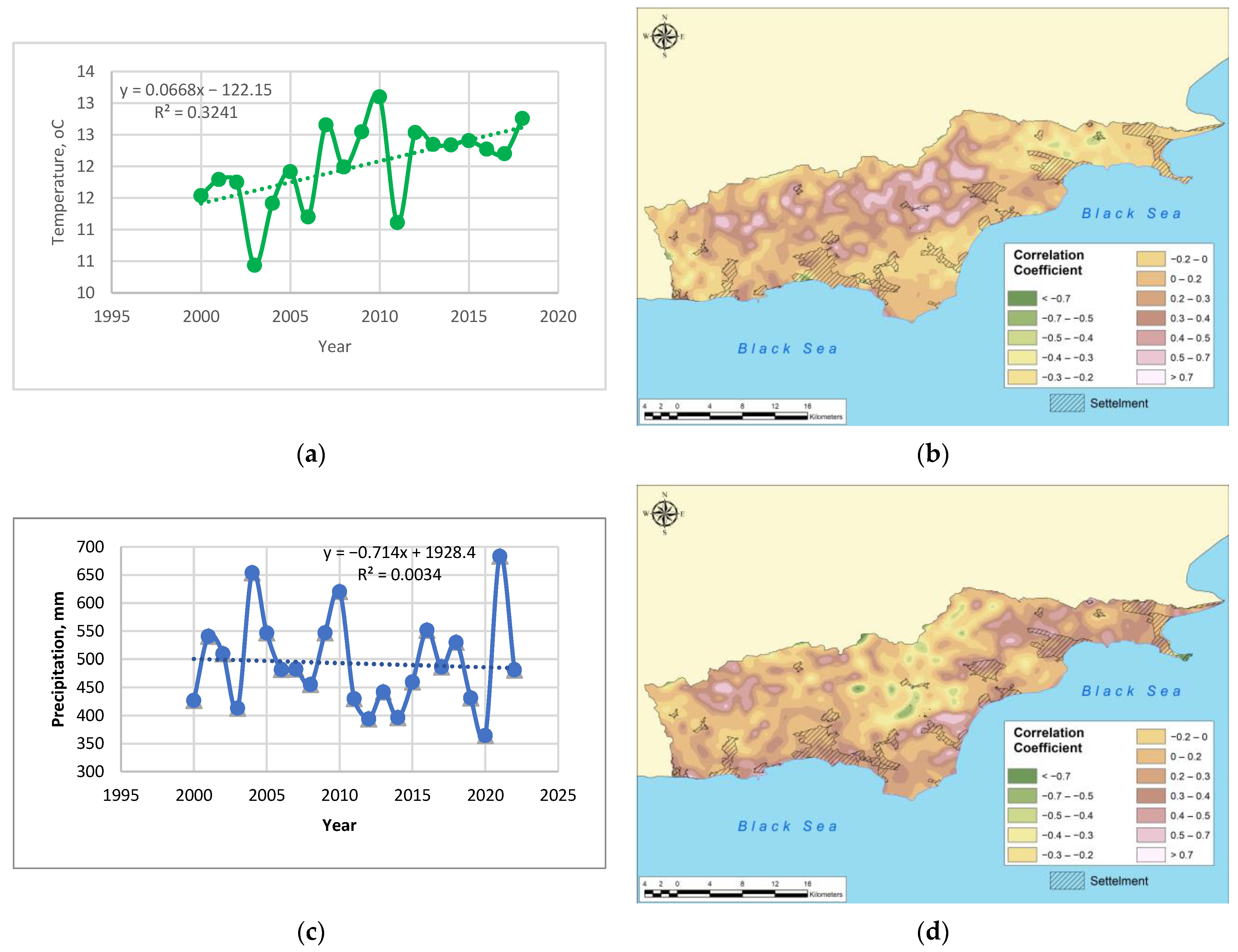
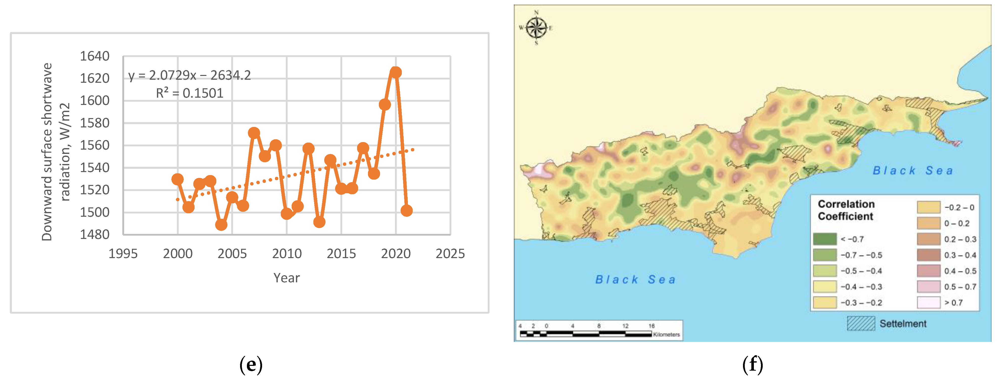
2.2.3. Temperature, Precipitation, and Solar Radiation Data

In recent years, extensive analysis has been conducted on various meteorological databases [61,62]. Spatial and temporal distribution data of air temperature, precipitation, and solar radiation fields were obtained from publicly available databases and published works by other researchers. Air temperature data within the Southeastern Crimea region were sourced from the ClimateEU database [63]. Precipitation and solar radiation data were retrieved using the Google Earth Engine platform from the CHIRPS [62] and ERA5-Land [64] datasets, respectively.

2.3. Methods

2.3.1. NDVI Trend Analysis

The analysis of NDVI trend changes within Southeastern Crimea was conducted for the entire study area and for each pixel of the NDVI raster. The linear regression model was extensively applied to assess the trend changes [38,65,66]. The assessment of NDVI changes over time was performed using the formula:

$$Slope=\frac{n\ast {NDVI}_i\ast {\sum }_{i=1}^{n}i-\sum _{i=1}^{n}i\ast \sum _{i=1}^{n}i}{n\ast \sum _{i=1}^n{i}^2-{\left({\sum }_{i=1}^{n}i\right)}^2}$$

(1)

where i—year; n—the number of years of observation; NDVI_i—NDVI value for year i.

Negative slope values indicate a decrease in NDVI values over time, while positive slope values indicate an increase in NDVI values over time. Additionally, the p-values were evaluated using the R Studio software (Version 2023.09.0+463; Posit PBC, Boston, MA, USA).

2.3.2. Coefficient of Variation

In order to evaluate the stability of NDVI values changes in the Southeastern Crimea region from 2001 to 2022, the coefficient of variation was calculated. The coefficient of variation was computed using the following formula:

$$CV=\frac{\sqrt{\frac{1}{n}{\sum }_{i=1}^n{\left({NDVI}_i-NDVI\right)}^2}}{NDVI}$$

(2)

where CV—coefficient of variation; n—the number of years in the study period; NDVI_i—NDVI value in year i; NDVI—the mean NDVI value for the entire study period [38].

The assessment of the coefficient of variation was performed using the R Studio software package for each pixel within the raster in the study region. Data values from the raster were extracted using the Quantum GIS software package (Version 3.16.16; Open Source Geospatial Foundation (OSGeo), Beaverton, OR, USA). To gauge the stability of changes, the coefficient of variation values was categorized into four classes based on the guidelines provided in [37]: very stable (CV ≤ 0.04), stable (0.04 < CV ≤ 0.08), slightly changed (0.08 < CV ≤ 0.12), and significantly changed (CV > 0.12) for each pixel in the analyzed image.

2.3.3. Hurst Index

In order to assess strategies for the development of forest ecosystems, the Hurst index was calculated as a means to forecast the evolution of temporal trends. The Hurst index is an effective method for identifying long-term dependencies in time series [29]. Detailed descriptions and calculations of the Hurst index can be found in several works [29,37,38]. The R Studio software package was utilized to simplify the calculations and determine the Hurst index for each pixel within the study region. Data values were obtained from the raster using the Quantum GIS software package. To calculate the Hurst index, data for 8-day periods of measurements of the MODIS space satellite were used. The calculation of the Hurst index was conducted using the R Studio programming environment, facilitated by the «pracma» library. This method involves the computation of the Hurst index through R/S analysis. To execute the R/S analysis, temporal series spanning the years 2001 to 2022 were individually subjected to a comprehensive examination for stationarity or non-stationarity. This evaluation was undertaken for each spatial cell. The Augmented Dickey–Fuller test, available within the R Studio environment and facilitated by the «tseries» library, was employed for this purpose. In instances where non-stationary time series were encountered, a sequence of transformations was applied to render them stationary. The R Studio program was employed for this transformation process, utilizing techniques such as logarithmization and differencing. These methods were strategically utilized to normalize variance and mitigate the presence of trends within the data. Upon the attainment of stationary time series, the computation of the Hurst index was undertaken through the utilization of the «pracma» library within R Studio. This index is derived from the R/S analysis and serves as an indicator of long-range dependence or persistence within the data. The calculated Hurst index values offer insights into the underlying temporal dynamics of the analyzed variables across different spatial cells. It is worth noting that this methodological approach aligns with a comprehensive workflow involving data preprocessing, statistical analysis, and computational procedures, all orchestrated within the R Studio environment.

2.3.4. Correlation Analysis

A correlation analysis was conducted to assess the influence of climatic factors, including annual precipitation, annual air temperatures, and annual solar radiation, on the average annual NDVI values within the Southeastern Crimea region. Correlation analysis is a widely used technique for examining the relationships between climate factors and NDVI values in various research regions worldwide [38,67,68]. Data on average annual NDVI values, air temperatures, precipitation, and solar radiation were obtained for a grid of points using the Quantum GIS software package (specifically, the Vector–Raster SAGA toolset). Each point within the presented grid of points functions as the central reference for a square, measuring 500 by 500 m. Consequently, these points are uniformly separated by a distance of 500 m from one another. The correlation calculation was performed according to the following formula:

$$R_{xy}=\frac{\sum _{i=1}^n\left[\left(x_i-x\right)\left(y_i-y\right)\right]}{\sqrt{{\sum }_{i=1}^n{\left(x_i-x\right)}^2{\sum }_{i=1}^n(y_i-y)}}$$

(3)

where R_xy—the correlation coefficient; n—the number of years in the study period; x and y—the factors used for the correlation analysis, representing the sample means of the variables [38].

The correlation assessment was performed using the R Studio software package. For the purpose of conducting correlation analysis, NDVI and climatic datasets spanning the years 2001 to 2022 were subjected to rigorous examination in terms of their stationarity or non-stationarity. This examination was undertaken utilizing the Augmented Dickey–Fuller test, a statistical method, within the computational environment of R Studio, specifically leveraging the «tseries» library. Time series exhibiting non-stationarity underwent a process of transformation into stationary series, accomplished through the application of logarithmic and differencing techniques. These techniques were instrumental in homogenizing variance across the temporal dimension and effecting the elimination of underlying trends. Subsequent to the attainment of stationary time series, correlation coefficients were computed individually for each temporal data point, a crucial step in elucidating the relationships between the NDVI and climatic variables. Upon generation of these correlation datasets, a seamless transition was effected into the ArcGIS software package (Version 10.8; ESRI, Redlands, CA, USA). Within this geospatial environment, an interpolation procedure, employing the well-regarded «Spline» method, was executed. This interpolation operation facilitated the derivation of intermediate values between discrete data points. Subsequently, cartographic representations were generated to visually articulate the spatial patterns emerging from the interpolated data, providing valuable insights into the dynamics of the studied variables across the geographical extent.

3. Results

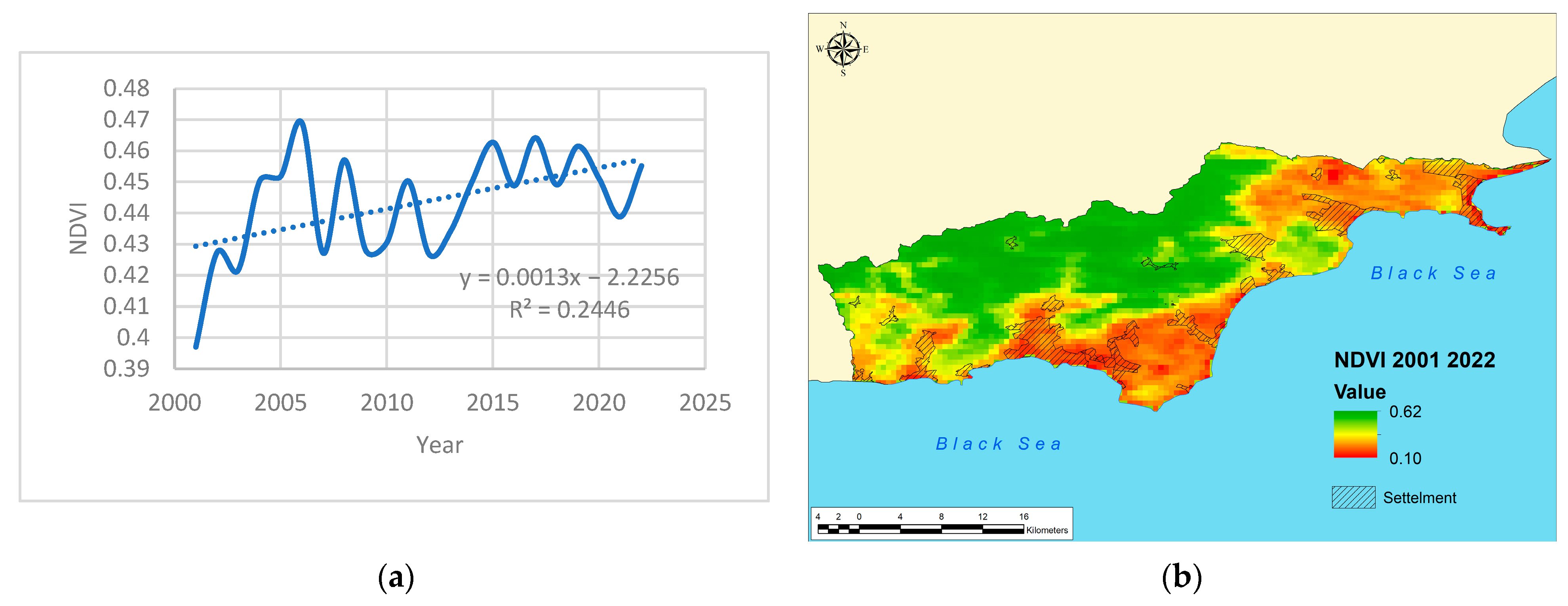
3.1. NDVI Dynamics in Southeastern Crimea

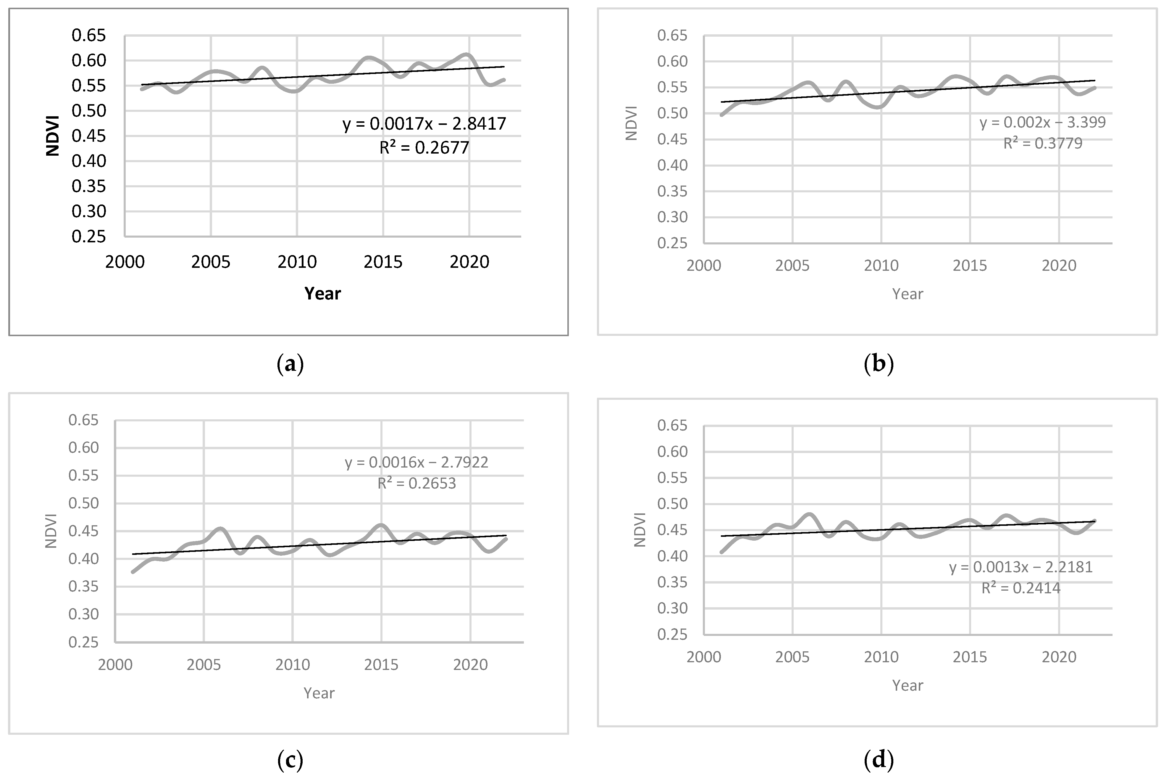
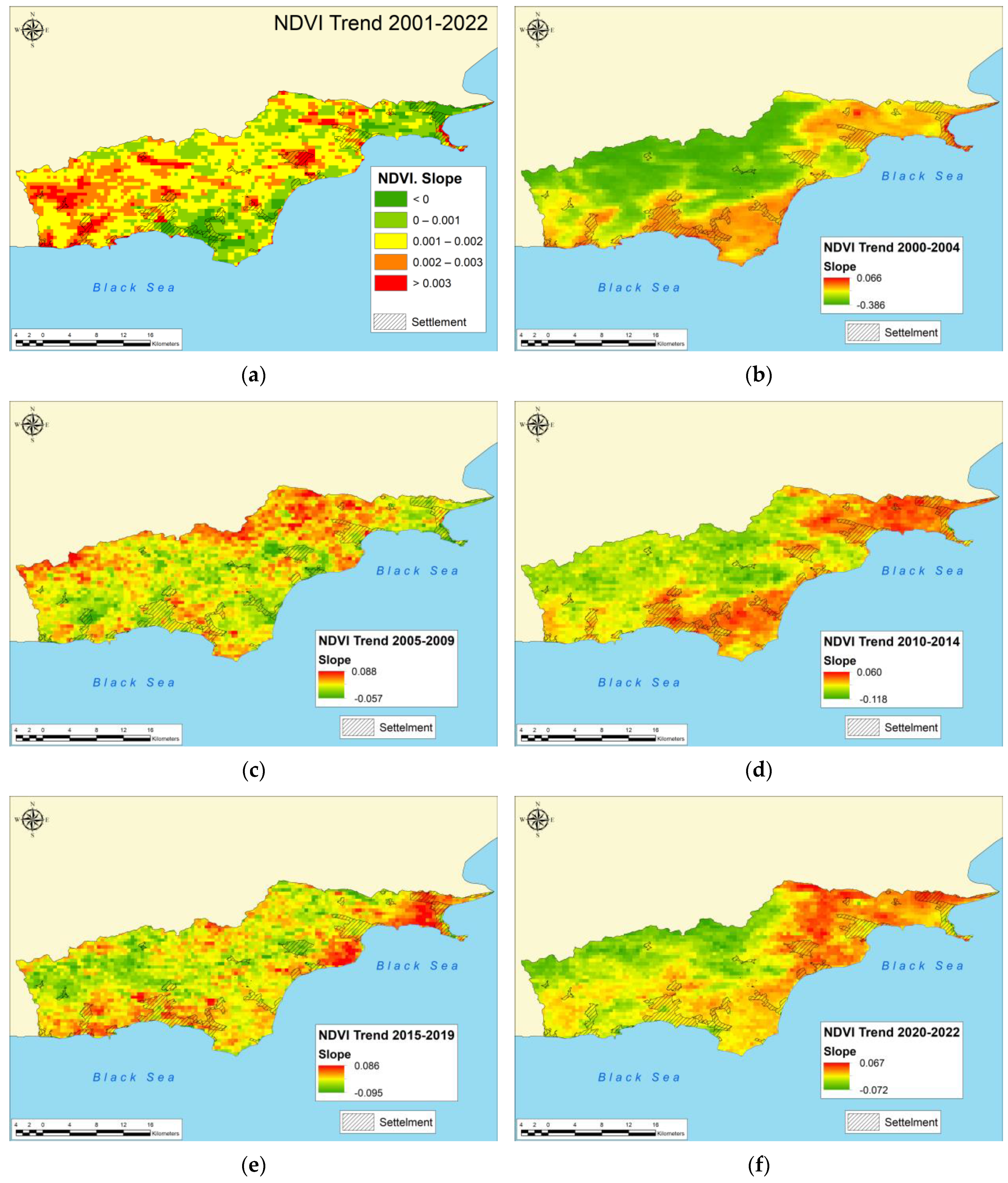
A consistent increase in the NDVI values has been observed in Southeastern Crimea from 2001 to 2022 (Figure 3 and Figure 4).

During the period from 2001 to 2022, the average NDVI value in Southeastern Crimea was 0.443. The highest average values were recorded in 2006, reaching 0.469, while the lowest values were observed in 2001–2002, at 0.397. In this context, the spatial distribution of the NDVI values within the investigated area from 2001 to 2022 exhibits a range of fluctuation spanning from 0.1 to 0.62. When comparing the annual average values for each year with the long-term mean, a clear trend of dividing the study period into two periods becomes apparent: before 2014, when the annual average NDVI values were consistently lower than the long-term mean, and after 2014, when the annual average NDVI values exceeded the long-term mean.

Figure 4 presents the dynamics of annual average NDVI values within the major vegetation communities in Southeastern Crimea.

Within the juniper forests, the average NDVI value was 0.43; within pubescent oak forests and their derivative hornbeam forests, it was 0.57; within the pubescent oak light forest in the complex with tomillares and savannoids, it was 0.54; and within the pubescent oak light forest in the complex with tomillares and savannoids, it was 0.45. Positive trends of increasing NDVI values are evident, particularly within the oak forests. From Figure 3 and Figure 4, it is evident that there is a trend of increasing NDVI values, indicating overall vegetation growth in Southeastern Crimea from 2001 to 2022. The distribution of annual average NDVI values within the major vegetation communities is presented in more detail in Figure 4, where the durmast oak with hornbeam and ash forests exhibit the highest NDVI values, while pubescent oak light forest in the complex with tomillares and savannoids show the lowest values.

In the southeastern region of Crimea, it is noteworthy that the peak of vegetation activity predominantly occurs in August. Figure 5 illustrates the monthly averages as well as the maximum and minimum values of the NDVI (Normalized Difference Vegetation Index) for the month of August, covering the period from 2001 to 2022.

Figure 6 presents the minimum, maximum, and average values of the NDVI vegetation index for various vegetation communities in Southeastern Crimea during August.

The graph illustrating maximum NDVI values across the extensive study area demonstrates a pronounced smoothing effect, thus limiting its ability to discern spatial and temporal differentiations within the analyzed region. Conversely, as we narrow down the spatial units under scrutiny and reduce their corresponding areas, the distinct differences become more apparent, rendering maximum data more meaningful. It is worth noting, however, that the practical application of maximum values should be exercised in light of the total count of maximum pixels within the designated study area. Meanwhile, the graph illustrating average NDVI values effectively captures discrepancies and offers the analytical and interpretive potential that underpins its utility. The smoothing effect evident in the graph of maximum values is an outcome of the representation of peak values of individual pixels, which can be spatially dispersed across various segments of the studied region, thereby rendering an incomplete reflection of the overarching patterns of change. A comparable circumstance applies to the distribution of minimum NDVI values in August, albeit, here, the scenario is characterized by a substantial dispersion of values, owing to certain pixels yielding negative NDVI values. Consequently, the application of analysis to both maximum and minimum values is, to a substantial extent, constrained. However, the validity of such analyses should be predicated on the proportional prevalence of minimum and maximum pixels within the examined region. We initially abstained from immediate utilization of minimum values due to the region’s characteristics, wherein minimum values could potentially encompass negative NDVI values attributed to the presence of water bodies and the dynamic sea coastline. Through comprehensive analysis of all NDVI values within the study area, we determined that for certain years, negative minimum values accounted for less than 0.1% of all data. A comparable pattern emerged in the distribution of maximum values. Specifically, we scrutinized NDVI values > 0.9 and ascertained that, for the majority of years, these values were either absent or constituted less than 0.5% of the complete dataset. However, while information about minimum and maximum values can serve to pinpoint localized growth or decline patterns, it is crucial to recognize that these values do not offer a holistic depiction of vegetation dynamics or the comprehensive operational landscape. Consequently, our study primarily relied upon the utilization of average NDVI values. This preference is rooted in the fact that minimum and maximum values, being isolated occurrences and accounting for a minute portion of the analyzed dataset, cannot adequately encompass the multifaceted character of the studied territory in Southeastern Crimea.

3.2. NDVI Trends

Significant spatial and temporal differentiation is observed within the territory of Southeastern Crimea, not only in the NDVI values themselves but also in the direction of their trends. Figure 7 illustrates the analysis of NDVI trend changes for the entire period from 2001 to 2022, as well as for five-year periods.

As shown in Figure 7a, there is an overall positive trend of NDVI values from 2001 to 2022, indicating an increase in vegetation biomass. However, negative trends are observed in specific areas near the cities of Sudak and Feodosia. When examining the spatial–temporal dynamics for five-year periods (Figure 7b–f), a complex pattern emerges within each spatial cell (pixel). During the period from 2001 to 2004, a noticeable decline in vegetation biomass and a decrease in NDVI values are observed in the central, northern, and northwestern parts of Southeastern Crimea. From 2005 to 2009, favorable conditions for vegetation growth are established in these areas, as indicated by positive values of the NDVI trend (Slope NDVI). Conversely, in areas where environmental conditions for vegetation growth were favorable from 2001 to 2004, conditions leading to a decrease in vegetation biomass are observed from 2005 to 2009. The situation in 2010–2014 is similar to that in 2001–2004. From 2015 to 2019, a complex pattern of growth and decline in vegetation is observed, yet the overall situation resembles the period of 2005–2009. Notably, starting from 2015, negative trends in NDVI values are observed in the western and northwestern parts of Southeastern Crimea, indicating a decrease in vegetation biomass. Therefore, quasi-five-year cycles can be identified, reflecting changes in vegetation cover in Southeastern Crimea.

If we consider the average values of the NDVI trend within the major vegetation communities, it can be observed that there is generally either an increase or a relatively stable trend in vegetation biomass (

Table 2. Average multi-year trend values within the vegetation communities of Southeastern Crimea from 2001 to 2022.

Variation Trend	Trend Prediction
	Minimum	Maximum	Average
Juniper forests	−0.0012	0.0060	0.0015
Beech forests with Stephen maple	0.0000	0.0040	0.0014
Durmast oak with hornbeam and ash forests	−0.0007	0.0050	0.0010
Pubescent oak forests and their derivative hornbeam forests	0.0000	0.0040	0.0014
Pubescent oak light forest in the complex with tomillares and savannoids	−0.0020	0.0050	0.0010
Forb-feather grass true submontane steppes	−0.0020	0.0103	0.0010
Orchards and vineyards in the place of pubescent oak forests and forb-feather grass genuine steppes	−0.0030	0.0050	0.0003
Cultivated areas under grain and tilled crops in the place of forb-feather grass steppes and pubescent oak forests	−0.0010	0.0030	0.0011
Urbocoenoses of inhabited localities	−0.0020	0.0050	0.0010

).

Anthropogenically created vegetation communities, such as gardens and vineyards, exhibit the least variability as they are artificially maintained throughout their existence due to human activities.

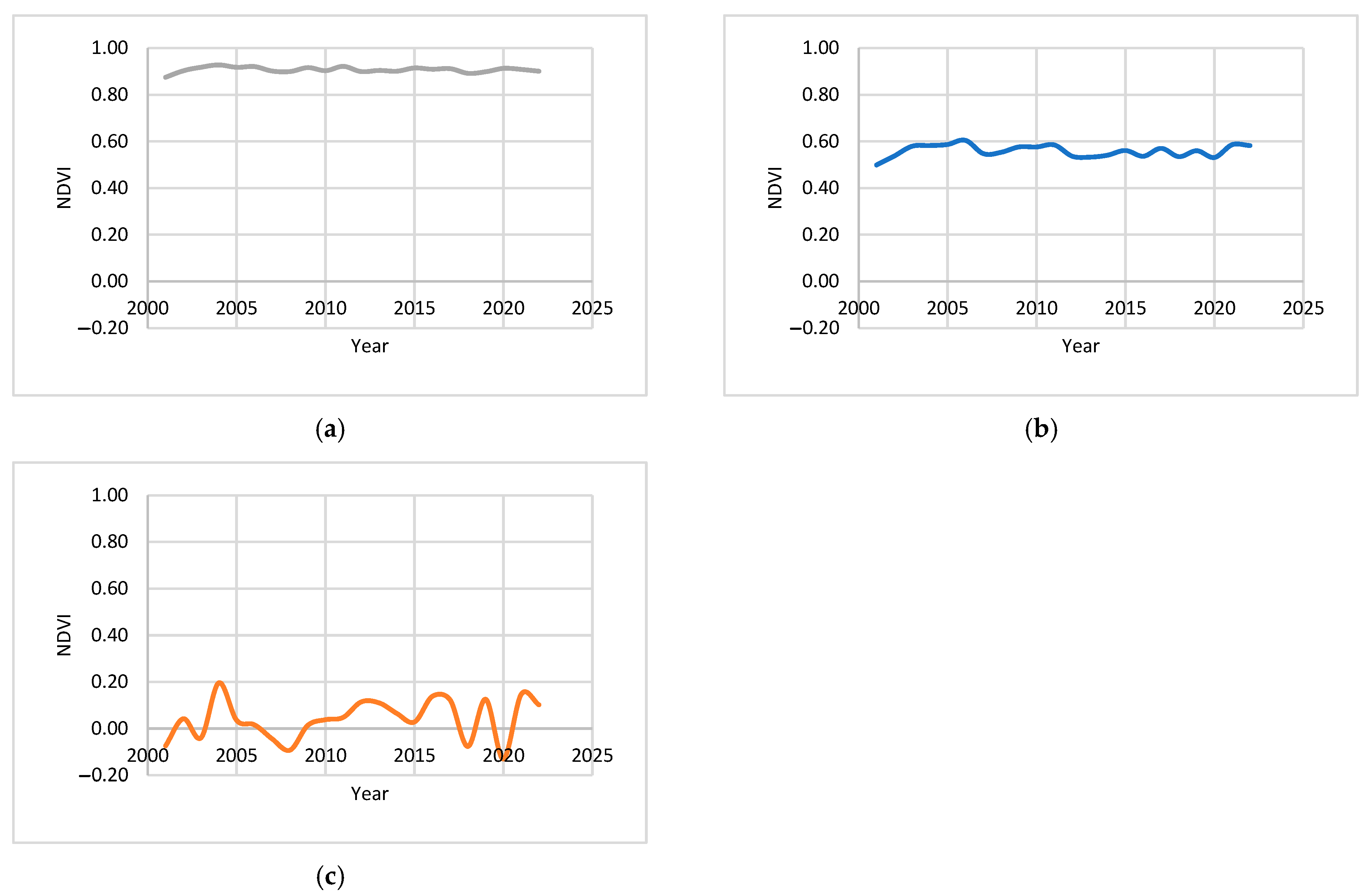
3.3. Coefficient of Variation

Let us now delve into a more detailed analysis of the coefficient of variation (CV) of NDVI values in Southeastern Crimea (Figure 8).

By assessing the CV of NDVI values, we were able to identify the most stable and highly variable areas within Southeastern Crimea. As shown in Figure 8, a significant portion of the study area exhibits a stable distribution of NDVI values. However, minor and significant fluctuations are predominantly observed in the southern and southeastern regions.

Table 3. Average multi-year changes in trend values within vegetation communities of Southeastern Crimea (2001–2022).

Variation Trend	CV
	Minimum	Maximum	Average
Juniper forests	0.04	0.21	0.06
Beech forests with Stephen maple	0.04	0.07	0.05
Durmast oak with hornbeam and ash forests	0.03	0.09	0.05
Pubescent oak forests and their derivative hornbeam forests	0.03	0.09	0.05
Pubescent oak light forest in the complex with tomillares and savannoids	0.03	4.43	0.06
Forb-feather grass true submontane steppes	0.04	2.90	0.08
Orchards and vineyards in the place of pubescent oak forests and forb-feather grass genuine steppes	0.03	0.44	0.08
Cultivated areas under grain and tilled crops in the place of forb-feather grass steppes and pubescent oak forests	0.06	0.13	0.09
Urbocoenoses of inhabited localities	0.04	0.19	0.08

presents the changes in the CV of NDVI within the vegetation communities of Southeastern Crimea from 2001 to 2022.

As can be observed from Table 3 and the Figure 8, the forest ecosystems exhibit greater stability compared with the steppe ecosystems and anthropogenically created agricultural lands and populated areas.

3.4. Hurst Index

The Hurst index provides a comprehensive assessment of vegetation variability and offers insights into forecasted changes. Figure 9 illuminates the spatial differentiation of Hurst index values in Southeastern Crimea, while

Table 4. Hurst index values within vegetation communities of Southeastern Crimea (2001–2022).

	Hurst Index
	Minimum	Maximum	Average
Juniper forests	0.49	0.85	0.73
Beech forests with Stephen maple	0.58	0.84	0.71
Durmast oak with hornbeam and ash forests	0.58	0.87	0.74
Pubescent oak forests and their derivative hornbeam forests	0.59	0.88	0.74
Pubescent oak light forest in the complex with tomillares and savannoids	0.56	0.93	0.76
Forb-feather grass true submontane steppes	0.54	0.94	0.76
Orchards and vineyards in the place of pubescent oak forests and forb-feather grass genuine steppes	0.59	0.93	0.77
Cultivated areas under grain and tilled crops in the place of forb-feather grass steppes and pubescent oak forests	0.65	0.87	0.74
Urbocoenoses of inhabited localities	0.61	0.94	0.78

furnishes a comprehensive account of the minimum, maximum, and mean Hurst index values pertaining to the principal vegetation communities within the same region.

It has been determined that the range of Hurst index values within Southeastern Crimea varies from 0.49 to 0.96, with a calculated mean value of 0.75. In the broader context of the Southeastern Crimea region, it is evident that the range of Hurst index values, calculated for NDVI data, exhibits pronounced spatial heterogeneity. The lowest Hurst index values are predominantly observed in the northernmost and northwestern sectors of the research area, while the highest values are consistently recorded in the coastal, southern, and southeastern regions. Notably, elevated Hurst index values are particularly prominent in proximity to urban settlements such as Shchebetovka, Kurortnoe, Sudak, Solnechnaya Dolina, and others.

3.5. Influence of Climatic Factors on NDVI Changes in Southeastern Crimea

To assess the impact of climatic factors on NDVI changes, an examination of the temporal dynamics of annual mean air temperature, precipitation, and solar radiation within Southeastern Crimea was conducted. Additionally, correlation coefficients were computed to determine the relationship between these factors and NDVI values (Figure 10).

The findings from Figure 10 reveal an upward trend in air temperature and solar radiation, accompanied by a slight reduction in precipitation levels in Southeastern Crimea. Notably, despite the modest decrease in precipitation, there exists a significant correlation between precipitation and NDVI values. Moreover, the correlation coefficients between NDVI and air temperature, as well as NDVI and solar radiation, indicate a moderate level of significance.

4. Discussion

Studying vegetation changes is a critical task as vegetation responds rapidly to various environmental factors. This is particularly important in regions with forests, which are valuable resources for multiple sectors. In this study, we analyzed the dynamics of NDVI and Hurst index values within the major vegetation communities of Southeastern Crimea.

Contrary to several published works [29,37,69], Southeastern Crimea does not exhibit significant variability in NDVI values. This can be attributed to the smaller study area compared with previous studies [69,70] and the prevalence of natural vegetation cover rather than contrasting or absent vegetation cover.

Although there are studies on NDVI dynamics for the Crimean Peninsula and its parts [42,43,71,72,73], Southeastern Crimea remains understudied. Notably, there are works assessing vegetation dynamics [74]. Fan et al. [70] calculated NDVI changes in the Crimean Peninsula within the Belt and Road Initiative region from 1982 to 2015. However, comparing their data with ours is challenging due to differences in spatial scales.

Comparing the Hurst index values of Southeastern Crimea with other regions worldwide, values below 0.5 prevail, similar to the Tibet Autonomous Region (China) [69] and Inner Mongolia (China) [29]. However, the Hurst index values (<0.4) indicate isolated centers of anti-sustainability within the downy oak forests of the Karadag Nature Reserve, supporting our previous findings [58]. Conversely, centers of instability predominantly occur at the boundaries of urban areas due to negative anthropogenic impact. Overall, studying NDVI dynamics and trends helps identify the most and least susceptible land and forest ecosystems. However, defining classes and boundaries presents challenges compared with previous studies [37,38], and alternative classification variants from [37,38] are not applicable in our research.

Forest ecosystems exhibit the highest correlation between vegetation cover and air temperature, precipitation, solar radiation, indicating favorable conditions for forest growth. However, the downy oak forests, located at the edge of their range, face unfavorable environmental conditions and cannot achieve their full potential in terms of green biomass. This underscores the presence of valuable and less vulnerable ecosystems within the Crimean Mountains.

Our findings are closely related to the data obtained by Han et al. [37] in Anhui Province (China), which indicates that the period around 2014–2015 marks a turning point in NDVI trend changes. However, unlike Han et al. [37], who attribute this to increased catastrophic natural phenomena, such as landslides and avalanches, this does not apply to Southeastern Crimea, where anthropogenic factors and global circulation processes play a significant role.

Considering vegetation-covered regions, NDVI values cannot be negative (unlike water surfaces), allowing us to analyze average values. However, due to pixel size limitations in satellite imagery, water bodies may be included, which are subject to boundary changes due to natural and anthropogenic factors, particularly relevant in the Crimean Peninsula [75]. Nevertheless, the influence on calculated NDVI values in our study region is minor since it belongs to water-deficient areas [58] and comprises numerous natural landscapes devoid of natural or human-created water bodies. Analyzing average annual NDVI values, as presented in Section 3, does not provide a clear understanding of change trends, necessitating more complex indicators to assess vegetation changes. The calculation of Hurst index and trend prediction values effectively addresses this research objective. Thus, the Hurst index proves to be a useful tool for analyzing future changes in regional NDVI, determining the stability or instability of trends, and predicting long-term vegetation cover changes.

The question of selecting the primary factor or combination of factors influencing vegetation growth within a specific research region remains unresolved. While temperature, precipitation, and solar radiation significantly contribute to the functioning of distinct vegetation communities in Southeastern Crimea, they are not the sole factors. Identifying and analyzing various environmental factors that influence vegetation functioning represent a promising research direction. The utilization of G.E. Hutchinson’s concept of multidimensional ecological niche [76] is highly relevant for studying vegetation dynamics. This framework provides valuable insights into the ecological requirements and responses of species within their respective environments. Simultaneously, our analysis has exclusively examined the impact of three climatic factors on vegetation change. Recognizing the intricate influence of climatic variables on the development and functioning of ecosystems and landscapes, it is imperative for future investigations to encompass a more comprehensive array of external factors. This expansion should not only encompass climatic variables but also extend to various other elements within the external environment.

When addressing the matter of selecting vegetation indices appropriate for the evaluation of vegetative landscape dynamics, the adoption of the NDVI demonstrates markedly heightened utility and applicability when compared with alternative vegetation indices. The preference for the NDVI vegetation index can primarily be attributed to its extensive prevalence and its capacity for facilitating inter-comparability among datasets generated by researchers. Esteemed scholars, including those referenced in sources [37,38,77], affirm that the NDVI possesses an enhanced capacity for delineating the growth status of vegetation, engendered by its heightened sensitivity to vegetative constituents. Accordingly, it is conventionally embraced as an efficacious evaluative metric for the surveillance of regional ecological systems. In the words of Li et al. [78], amongst the entire gamut of vegetation indices, the NDVI evinces a robust correlation with net primary productivity (NPP), canopy extent, and biomass. This confluence of attributes enables it to aptly encapsulate and gauge the trajectory of vegetative growth. Consequently, it assumes prominence within investigations into the temporal vicissitudes of regional vegetative ecosystems.

Concurrently, an extensive array of vegetation indices, amenable to computation based on satellite-derived imagery, exists. For instance, the ratio vegetation index (RVI) [79], infrared percentage vegetation index (IPVI) [80], and transformed vegetation index (TVI) [81], while relying on identical satellite image channels as NDVI for computation, are integrally linked to NDVI. Their autonomous consideration, dissociated from the NDVI framework, is bereft of practical import. Notably, NDVI’s ascendancy is underscored by its scalar range, spanning from −1 to 1, unlike the ratio vegetation index (RVI) [79] or the difference vegetation index (DVI) [82], both characterized by dimensionality sans constraints, thereby exacerbating the intricacies attendant upon inter-data comparison and interpretation.

Pioneers in the field, including Huete et al. [83] and Elvidge and Lyon [84], have underscored the substantive influence of soil cover upon vegetation indices. However, it is germane to apprehend that the sensitivity of all vegetation indices to the overprint of soil cover and unadorned tracts bereft of vegetation is ubiquitous. In the context of an examined image pixel, NDVI is amenable to calculation, encapsulating the entwined characteristics of soil and aquatic features. Yet, with the burgeoning of vegetative constituents within the confines of this pixel, the NDVI amplitude burgeons in tandem, reflective of the enshrouding of soil domains or the supplanting of erstwhile aquatic expanses. Moreover, certain vegetation indices encompass considerations of both soil and ground surface influence. Instances thereof comprise the transformed soil adjusted vegetation index (TSAVI) [85], modified soil adjusted vegetation index (MSAVI) [86], and enhanced vegetation index (EVI) [87]. Their deployment, however, is confined to locales characterized by a luxuriant mantle of vegetation, encompassing the studied region. This confinement emanates from the intricate constraints impeding precise delimitation of soil constants, as delineated extensively in the monograph [88]. Under these circumstances, the predilection for NDVI prevails, owing to its optimized resonance with vegetative profusion, emblematic of Southeastern Crimea’s ecological tapestry. Although the integration of the enhanced vegetation index (EVI) was contemplated during the preparatory stages of inquiry, its notable proclivity for inaccuracy precluded its integration into the investigative paradigm. Furthermore, as underscored in the discourse [42], EVI values evince marginal alignment with alternative vegetation index metrics (most notably NDVI). The calculus of EVI betrayed an elevated susceptibility to terrain topography, a consideration that becomes particularly salient in the backdrop of the study area’s intricate and variegated topographical terrain, thereby giving rise to pronounced disparities [89]. Martín-Ortega et al. [90] elucidate the fact that the enhanced vegetation index (EVI) displays enhanced sensitivity to biophysical parameters such as leaf area index (LAI), and is notably impacted by atmospheric conditions to a greater extent than the conventional normalized difference vegetation index (NDVI), owing to the inherent non-ratio nature of EVI. Moreover, empirical evidence underscores that EVI exhibits a heightened degree of responsiveness, approximately five times greater than NDVI, towards fluctuations in near-infrared reflectance (NIR). In contrast, Martín-Ortega et al. [90] observe that the ratio-based formulation of NDVI confers the ability to effectively ameliorate a substantial quantum of perturbations stemming from dynamic solar angles, topographical variations, cloud-induced interference, and shading effects. This inherent property endows NDVI with enhanced robustness against alterations in luminous conditions.

The incorporation of vegetation indices calibrated to ameliorate the influence of soil cover necessitates a nuanced incorporation of regional idiosyncrasies, concomitant with the integration of sundry correction coefficients. These coefficients, inevitably variably distributed across raster cells due to the heterogeneity characterizing soil and terrestrial substrate, preclude universal homogenization. Ergo, the electivity for NDVI culminates in its conspicuously salient relevance for the entire Crimea Peninsula, and Southeastern Crimea, specifically, as manifestly chronicled in scholarly contributions [73,74,91]. The ramifications of soil characteristics at localized and regional research junctures command prodigious endeavor and temporal investment in the context of field and laboratory spectroscopic evaluations of soil. Analogous undertakings, frequently conducted to fine-tune global models and extricate regional particularities across assorted scientific disciplines leveraging remote terrestrial sensing datasets, are amply discernible in the extant corpus [92,93].

Another crucial aspect to consider in the analysis of NDVI value changes and the calculation of the Hurst index was the transformation of time series into a stationary form. This was necessitated by the fact that one of the most widely used methods for calculating the Hurst exponent is the R/S analysis. Holl et al. [94] point out that in the natural world, real-life data often contains inherent trends that render the series nonstationary, thereby rendering the R/S analysis inappropriate. This phenomenon arises from the fact that the R/S analysis can be applied to series that exhibit a degree of stationarity on mean [95]. Furthermore, as indicated by reference [96], it is imperative to consider that in order to compute the Hurst index, the length of the observational series should encompass a minimum of 256 measurements.

Another limitation of this study is the paucity of data and the challenges associated with the geospatial processing of climatic characteristics within Southeastern Crimea. We concur with the findings of Han et al. [37], who highlighted that different interpolation methods for climatic data can lead to divergent raster fields of climate factors.

Furthermore, it is important to recognize the potential use of more detailed satellite imagery with higher spatial resolution (e.g., Sentinel-2 with a resolution of 10 m/pixel), in contrast to the MODIS data employed in this study. Nevertheless, the use of MODIS satellite imagery was primarily driven by its extensive spatial and temporal coverage, despite its lower resolution. As satellite imaging frequency increases in the future, endeavors should be made to enhance data quality and obtain higher-resolution datasets. Additionally, it is imperative to improve the quality of available open climatic data, which currently can only be spatially correlated with MODIS satellite imagery. Another pivotal constraint inherent to this research pertains to the observation duration, a parameter dictated by the accessibility of data procured from orbiting satellites. In the case of the MODIS satellite, as delineated within our investigation, the dataset spans from 2001 onwards. In the event alternative spaceborne satellites are employed for the acquisition of requisite multispectral satellite imagery, instrumental for NDVI computations, the temporal extent of observational records could conceivably expand (as in the case of Landsat) or conversely contract (as exemplified by Sentinel-2). Another salient consideration in research lies in the recognition that the computation of NDVI values, executed across diverse satellite platforms and software suites (such as MODIS, Landsat, Sentinel-2, among others), inherently yields variations due to discrepant imaging epochs. The challenge of coherently aligning images for a specific temporal point compounds this variation. Moreover, even in instances where alignment is achieved, the fact remains that MODIS, Landsat, Sentinel-2, and analogous satellite sensors capture imagery within distinct spectral ranges. Consequently, the comparative analysis of resultant data emerges as an intricate endeavor. It is imperative to duly acknowledge this intricacy as a prospective stipulation shaping the contours of the study’s limitations.

Addressing these limitations and incorporating advanced data sources and analytical methods will contribute to a more comprehensive understanding of vegetation dynamics and the underlying environmental factors in Southeastern Crimea.

5. Conclusions

Vegetation cover serves as a crucial indicator of the environmental condition and offers valuable insights into ecosystem health. It plays a significant role in assessing environmental parameters, monitoring anthropogenic activities, evaluating ecosystem services, and understanding forest landscape functions. Understanding the dynamics of vegetation change is essential for effective conservation planning, species preservation, sustainable forest management, and protection. However, it is crucial to recognize the conflicting interests between economic exploitation of forests and environmental conservation efforts.

To achieve a balance between economic development and environmental preservation, it is necessary to comprehend the impact of human activities and climate change on vegetation cover. Future research should focus on comprehensive analysis and comparison of various vegetation indices beyond NDVI, exploring functional characteristics of vegetation such as primary productivity and carbon sequestration, integrating NDVI calculations with other remote sensing techniques such as unmanned aerial vehicle (UAV) imagery for precise assessments of canopy structure and three-dimensional characteristics, and investigating localized redistribution of key meteorological parameters. An auspicious avenue of research lies in the utilization of detrended fluctuation analysis techniques for the assessment of NDVI dynamics.

The utilization of geospatial analysis and remote sensing techniques enables the acquisition of extensive spatial information regarding vegetation dynamics and its correlation with climate change. This knowledge facilitates improved environmental planning, decision making, and the implementation of sustainable practices for conservation and development.

Studying vegetation dynamics provides valuable insights into environmental changes and plays a pivotal role in preserving natural ecosystems, managing resources, and striving towards sustainable development objectives.

References

1. Miles, J. Vegetation Dynamics; Springer Science & Business Media: Dordrecht, The Netherlands, 1979; 80p. [Google Scholar] [CrossRef]
2. Zhou, Z.; Ding, Y.; Shi, H.; Cai, H.; Fu, Q.; Liu, S.; Li, T. Analysis and prediction of vegetation dynamic changes in China: Past, present and future. Ecol. Indic. 2020, 117, 106642. [Google Scholar] [CrossRef]
3. Piao, S.; Fang, J.; Zhou, L.; Zhu, B.; Tan, K.; Tao, S. Changes in vegetation net primary productivity from 1982 to 1999 in China. Glob. Biogeochem. Cycles 2005, 19, 2. [Google Scholar] [CrossRef]
4. Mayeux, H.S.; Johnson, H.B.; Polley, H.W. Global change and vegetation dynamics. In Noxious Range Weeds, 1st ed.; CRC Press: Boca Raton, FL, USA, 1992; pp. 62–74. [Google Scholar] [CrossRef]
5. Brancalion, P.H.; Garcia, L.C.; Loyola, R.; Rodrigues, R.R.; Pillar, V.D.; Lewinsohn, T.M. A critical analysis of the Native Vegetation Protection Law of Brazil (2012): Updates and ongoing initiatives. Nat. Conserv. 2016, 14, 1–15. [Google Scholar] [CrossRef]
6. Opoku, A. Biodiversity and the built environment: Implications for the Sustainable Development Goals (SDGs). Resour. Conserv. Recycl. 2019, 141, 1–7. [Google Scholar] [CrossRef]
7. Li, Z.; Chen, Y.; Li, W.; Deng, H.; Fang, G. Potential impacts of climate change on vegetation dynamics in Central Asia. J. Geophys. Res. Atmos. 2015, 120, 12345–12356. [Google Scholar] [CrossRef]
8. Jiang, L.; Bao, A.; Guo, H.; Ndayisaba, F. Vegetation dynamics and responses to climate change and human activities in Central Asia. Sci. Total Environ. 2017, 599, 967–980. [Google Scholar] [CrossRef]
9. Verrall, B.; Pickering, C.M. Alpine vegetation in the context of climate change: A global review of past research and future directions. Sci. Total Environ. 2020, 748, 141344. [Google Scholar] [CrossRef]
10. Kalisa, W.; Igbawua, T.; Henchiri, M.; Ali, S.; Zhang, S.; Bai, Y.; Zhang, J. Assessment of climate impact on vegetation dynamics over East Africa from 1982 to 2015. Sci. Rep. 2019, 9, 16865. [Google Scholar] [CrossRef]
11. Shen, P.; Zhang, L.M.; Fan, R.L.; Zhu, H.; Zhang, S. Declining geohazard activity with vegetation recovery during first ten years after the 2008 Wenchuan earthquake. Geomorphology 2020, 352, 106989. [Google Scholar] [CrossRef]
12. Malawani, M.N.; Lavigne, F.; Gomez, C.; Mutaqin, B.W.; Hadmoko, D.S. Review of Local and Global Impacts of Volcanic Eruptions and Disaster Management Practices: The Indonesian Example. Geosciences 2021, 11, 109. [Google Scholar] [CrossRef]
13. Thonicke, K.; Venevsky, S.; Sitch, S.; Cramer, W. The role of fire disturbance for global vegetation dynamics: Coupling fire into a Dynamic Global Vegetation Model. Glob. Ecol. Biogeogr. 2001, 10, 661–677. [Google Scholar] [CrossRef]
14. Touré, A.A.; Tidjani, A.D.; Rajot, J.L.; Marticorena, B.; Bergametti, G.; Bouet, C.; Garba, Z. Dynamics of wind erosion and impact of vegetation cover and land use in the Sahel: A case study on sandy dunes in southeastern Niger. Catena 2019, 177, 272–285. [Google Scholar] [CrossRef]
15. Tang, C.; Liu, Y.; Li, Z.; Guo, L.; Xu, A.; Zhao, J. Effectiveness of vegetation cover pattern on regulating soil erosion and runoff generation in red soil environment, southern China. Ecol. Indic. 2021, 129, 107956. [Google Scholar] [CrossRef]
16. Chen, J.; Shao, Z.; Huang, X.; Cai, B.; Zheng, X. Assessing the impact of floods on vegetation worldwide from a spatiotemporal perspective. J. Hydrol. Hydrol. 2023, 622, 129715. [Google Scholar] [CrossRef]
17. Hu, T.; Smith, R.B. The Impact of Hurricane Maria on the Vegetation of Dominica and Puerto Rico Using Multispectral Remote Sensing. Remote Sens. 2018, 10, 827. [Google Scholar] [CrossRef]
18. Olivero, J.; Fa, J.E.; Real, R.; Márquez, A.L.; Farfán, M.A.; Vargas, J.M.; Gaveau, D.; Salim, M.A.; Park, D.; Suter, J.; et al. Recent loss of closed forests is associated with Ebola virus disease outbreaks. Sci. Rep. 2017, 7, 14291. [Google Scholar] [CrossRef]
19. Romero-Alvarez, D.; Escobar, L.E. Vegetation loss and the 2016 Oropouche fever outbreak in Peru. Mem. Inst. Oswaldo Cruz 2017, 112, 292–298. [Google Scholar] [CrossRef]
20. McAlpine, C.A.; Fensham, R.J.; Temple-Smith, D.E. Biodiversity conservation and vegetation clearing in Queensland: Principles and thresholds. Rangel. J. 2002, 24, 36–55. [Google Scholar] [CrossRef]
21. Nogueira, E.M.; Yanai, A.M.; Fonseca, F.O.R.; Fearnside, P.M. Carbon stock loss from deforestation through 2013 in Brazilian Amazonia. Glob. Chang. Biol. 2015, 21, 1271–1292. [Google Scholar] [CrossRef]
22. Mederski, P.; Jakubowski, M.; Karaszewski, Z. The Polish landscape changing due to forest policy and forest management. iForest Biogeosciences For. 2009, 2, 140–142. [Google Scholar] [CrossRef]
23. Yurova, A.Y.; Volodin, E.M. Coupled simulation of climate and vegetation dynamics. Izv. Atmos. Ocean. Phys. 2011, 47, 531–539. [Google Scholar] [CrossRef]
24. Hobbs, R.J. Remote Sensing of Spatial and Temporal Dynamics of Vegetation. In Remote Sensing of Biosphere Functioning; Hobbs, R.J., Mooney, H.A., Eds.; Springer: New York, NY, USA, 1990; pp. 203–219. [Google Scholar] [CrossRef]
25. Sun, G.Q.; Li, L.; Li, J.; Liu, C.; Wu, Y.P.; Gao, S.; Wang, Z.; Feng, G.L. Impacts of climate change on vegetation pattern: Mathematical modelling and data analysis. Phys. Life Rev. 2022, 43, 239–270. [Google Scholar] [CrossRef] [PubMed]
26. Potapov, P.; Hansen, M.C.; Kommareddy, I.; Kommareddy, A.; Turubanova, S.; Pickens, A.; Adusei, B.; Tyukavina, A.; Ying, Q. Landsat Analysis Ready Data for Global Land Cover and Land Cover Change Mapping. Remote Sens. 2020, 12, 426. [Google Scholar] [CrossRef]
27. Liu, B.; Pan, L.; Qi, Y.; Guan, X.; Li, J. Land Use and Land Cover Change in the Yellow River Basin from 1980 to 2015 and Its Impact on the Ecosystem Services. Land 2021, 10, 1080. [Google Scholar] [CrossRef]
28. Abdullah, A.Y.M.; Masrur, A.; Adnan, M.S.G.; Baky, M.A.A.; Hassan, Q.K.; Dewan, A. Spatio-Temporal Patterns of Land Use/Land Cover Change in the Heterogeneous Coastal Region of Bangladesh between 1990 and 2017. Remote Sens. 2019, 11, 790. [Google Scholar] [CrossRef]
29. Kang, Y.; Guo, E.; Wang, Y.; Bao, Y.; Bao, Y.; Mandula, N. Monitoring Vegetation Change and Its Potential Drivers in Inner Mongolia from 2000 to 2019. Remote Sens. 2021, 13, 3357. [Google Scholar] [CrossRef]
30. Gandhi, G.M.; Parthiban, B.S.; Thummalu, N.; Christy, A. NDVI: Vegetation change detection using remote sensing and gis—A case study of Vellore District. Procedia Comput. Sci. 2015, 57, 1199–1210. [Google Scholar] [CrossRef]
31. Waseem, S.; Khayyam, U. Loss of vegetative cover and increased land surface temperature: A case study of Islamabad, Pakistan. J. Clean. Prod. 2019, 234, 972–983. [Google Scholar] [CrossRef]
32. Jełowicki, Ł.; Sosnowicz, K.; Ostrowski, W.; Osińska-Skotak, K.; Bakuła, K. Evaluation of Rapeseed Winter Crop Damage Using UAV-Based Multispectral Imagery. Remote Sens. 2020, 12, 2618. [Google Scholar] [CrossRef]
33. Keshta, A.E.; Riter, J.C.A.; Shaltout, K.H.; Baldwin, A.H.; Kearney, M.; Sharaf El-Din, A.; Eid, E.M. Loss of Coastal Wetlands in Lake Burullus, Egypt: A GIS and Remote-Sensing Study. Sustainability 2022, 14, 4980. [Google Scholar] [CrossRef]
34. Li, C.; Jia, X.; Zhu, R.; Mei, X.; Wang, D.; Zhang, X. Seasonal Spatiotemporal Changes in the NDVI and Its Driving Forces in Wuliangsu Lake Basin, Northern China from 1990 to 2020. Remote Sens. 2023, 15, 2965. [Google Scholar] [CrossRef]
35. Long, Q.; Wang, F.; Ge, W.; Jiao, F.; Han, J.; Chen, H.; Roig, F.A.; Abraham, E.M.; Xie, M.; Cai, L. Temporal and Spatial Change in Vegetation and Its Interaction with Climate Change in Argentina from 1982 to 2015. Remote Sens. 2023, 15, 1926. [Google Scholar] [CrossRef]
36. Dhillon, M.S.; Kübert-Flock, C.; Dahms, T.; Rummler, T.; Arnault, J.; Steffan-Dewenter, I.; Ullmann, T. Evaluation of MODIS, Landsat 8 and Sentinel-2 Data for Accurate Crop Yield Predictions: A Case Study Using STARFM NDVI in Bavaria, Germany. Remote Sens. 2023, 15, 1830. [Google Scholar] [CrossRef]
37. Han, W.; Chen, D.; Li, H.; Chang, Z.; Chen, J.; Ye, L.; Liu, S.; Wang, Z. Spatiotemporal Variation of NDVI in Anhui Province from 2001 to 2019 and Its Response to Climatic Factors. Forests 2022, 13, 1643. [Google Scholar] [CrossRef]
38. Jiang, F.; Deng, M.; Long, Y.; Sun, H. Spatial pattern and dynamic change of vegetation greenness from 2001 to 2020 in Tibet, China. Front. Plant Sci. 2022, 13, 892625. [Google Scholar] [CrossRef] [PubMed]
39. Li, M.; Yan, Q.; Li, G.; Yi, M.; Li, J. Spatio-Temporal Changes of Vegetation Cover and Its Influencing Factors in Northeast China from 2000 to 2021. Remote Sens. 2022, 14, 5720. [Google Scholar] [CrossRef]
40. Tong, S.; Zhang, J.; Bao, Y.; Lai, Q.; Lian, X.; Li, N.; Bao, Y. Analyzing vegetation dynamic trend on the Mongolian Plateau based on the hurst exponent and influencing factors from 1982–2013. J. Geogr. Sci. 2018, 28, 595–610. [Google Scholar] [CrossRef]
41. Saikia, A. NDVI variability in North East India. Scott. Geogr. J. 2009, 125, 195–213. [Google Scholar] [CrossRef]
42. Shibani, N.; Pandey, A.; Satyam, V.K.; Bhari, J.S.; Karimi, B.A.; Gupta, S.K. Study on the variation of NDVI, SAVI and EVI indices in Punjab State, India. IOP Conf. Ser. Earth Environ. Sci. 2023, 1110, 012070. [Google Scholar] [CrossRef]
43. Johnson, D.M.; Rosales, A.; Mueller, R.; Reynolds, C.; Frantz, R.; Anyamba, A.; Pak, E.; Tucker, C. USA Crop Yield Estimation with MODIS NDVI: Are Remotely Sensed Models Better than Simple Trend Analyses? Remote Sens. 2021, 13, 4227. [Google Scholar] [CrossRef]
44. Ghorbanian, A.; Mohammadzadeh, A.; Jamali, S. Linear and Non-Linear Vegetation Trend Analysis throughout Iran Using Two Decades of MODIS NDVI Imagery. Remote Sens. 2022, 14, 3683. [Google Scholar] [CrossRef]
45. Pimentel, D.; McNair, M.; Buck, L.; Pimentel, M.; Kamil, J. The Value of Forests to World Food Security. Hum. Ecol. 1997, 25, 91–120. [Google Scholar] [CrossRef]
46. Pearce, D.W. The economic value of forest ecosystems. Ecosyst. Health 2001, 7, 284–296. [Google Scholar] [CrossRef]
47. Grantham, H.S.; Duncan, A.; Evans, T.D.; Jones, K.R.; Beyer, H.L.; Schuster, R.; Walston, J.; Ray, J.C.; Robinson, J.G.; Callow, M.; et al. Anthropogenic modification of forests means only 40% of remaining forests have high ecosystem integrity. Nat. Commun. 2020, 11, 5978. [Google Scholar] [CrossRef]
48. Fearnside, P.M.; Guimarães, W.M. Carbon uptake by secondary forests in Brazilian Amazonia. For. Ecol. Manag. 1996, 80, 35–46. [Google Scholar] [CrossRef]
49. Landuyt, D.; De Lombaerde, E.; Perring, M.P.; Hertzog, L.R.; Ampoorter, E.; Maes, S.L.; De Frenne, P.; Ma, S.; Proesmans, W.; Blondeel, H.; et al. The functional role of temperate forest understorey vegetation in a changing world. Glob. Chang. Biol. 2019, 25, 3625–3641. [Google Scholar] [CrossRef]
50. Wieczynski, D.J.; Boyle, B.; Buzzard, V.; Duran, S.M.; Henderson, A.N.; Hulshof, C.M.; Kerkhoff, A.J.; McCarthy, M.C.; Michaletz, S.T.; Swenson, N.G.; et al. Climate shapes and shifts functional biodiversity in forests worldwide. Proc. Natl. Acad. Sci. USA 2019, 116, 587–592. [Google Scholar] [CrossRef]
51. Riccioli, F.; Marone, E.; Boncinelli, F.; Tattoni, C.; Rocchini, D.; Fratini, R. The recreational value of forests under different management systems. New For. 2019, 50, 345–360. [Google Scholar] [CrossRef]
52. Negrón-Juárez, R.I.; Holm, J.A.; Marra, D.M.; Rifai, S.W.; Riley, W.J.; Chambers, J.Q.; Koven, C.D.; Knox, R.G.; E McGroddy, M.; Di Vittorio, A.V.; et al. Vulnerability of Amazon forests to storm-driven tree mortality. Environ. Res. Lett. 2018, 13, 054021. [Google Scholar] [CrossRef]
53. Hutyra, L.R.; Munger, J.W.; Nobre, C.A.; Saleska, S.R.; Vieira, S.A.; Wofsy, S.C. Climatic variability and vegetation vulnerability in Amazonia. Geophys. Res. Lett. 2005, 32, L24712. [Google Scholar] [CrossRef]
54. Laurance, W.F.; Campbell, M.J.; Alamgir, M.; Mahmoud, M.I. Road expansion and the fate of Africa’s tropical forests. Front. Ecol. Evol. 2017, 5, 75. [Google Scholar] [CrossRef]
55. Potapov, P.; Hansen, M.C.; Laestadius, L.; Turubanova, S.; Yaroshenko, A.; Thies, C.; Smith, W.; Zhuravleva, I.; Komarova, A.; Minnemeyer, S.; et al. The last frontiers of wilderness: Tracking loss of intact forest landscapes from 2000 to 2013. Sci. Adv. 2017, 3, e1600821. [Google Scholar] [CrossRef] [PubMed]
56. Van Khuc, Q.; Tran, B.Q.; Meyfroidt, P.; Paschke, M.W. Drivers of deforestation and forest degradation in Vietnam: An exploratory analysis at the national level. For. Policy Econ. 2018, 90, 128–141. [Google Scholar] [CrossRef]
57. Fan, L.; Wigneron, J.P.; Ciais, P.; Chave, J.; Brandt, M.; Sitch, S.; Yue, C.; Bastos, A.; Li, X.; Qin, Y.; et al. Siberian carbon sink reduced by forest disturbances. Nat. Geosci. 2023, 16, 56–62. [Google Scholar] [CrossRef]
58. Gorbunov, R.; Tabunshchik, V.; Gorbunova, T.; Safonova, M. Water Balance Components of Sub-Mediterranean Downy Oak Landscapes of Southeastern Crimea. Forests 2022, 13, 1370. [Google Scholar] [CrossRef]
59. Bokov, V.A. (Ed.) Landscape and Geophysical Conditions for the Growth of Forests in the Southeastern Part of the Mountainous Crimea; Tavria-Plus: Simferopol, Crimea, 2001; 133p. [Google Scholar]
60. Rudenko, L.G. (Ed.) National Atlas of Ukraine; Cartography: Kiev, Ukraine, 2007; 435p. [Google Scholar]
61. Banerjee, A.; Chen, R.E.; Meadows, M.; Singh, R.B.; Mal, S.; Sengupta, D. An Analysis of Long-Term Rainfall Trends and Variability in the Uttarakhand Himalaya Using Google Earth Engine. Remote Sens. 2020, 12, 709. [Google Scholar] [CrossRef]
62. Funk, C.; Peterson, P.; Landsfeld, M.; Pedreros, D.; Verdin, J.; Shukla, S.; Husak, G.; Rowland, J.; Harrison, L.; Hoell, A.; et al. The climate hazards infrared precipitation with stations—A new environmental record for monitoring extremes. Sci. Data 2015, 2, 150066. [Google Scholar] [CrossRef]
63. Marchi, M.; Castellanos-Acuna, D.; Hamann, A.; Wang, T.; Ray, D.; Menzel, A. ClimateEU, scale-free climate normals, historical time series, and future projections for Europe. Sci. Data 2020, 7, 428. [Google Scholar] [CrossRef]
64. Muñoz Sabater, J. ERA5-Land Monthly Averaged Data from 1981 to Present. Copernicus Climate Change Service (C3S) Climate Data Store (CDS). Available online: https://cds.climate.copernicus.eu/cdsapp#!/dataset/10.24381/cds.68d2bb30?tab=overview (accessed on 7 July 2023).
65. Ndayisaba, F.; Guo, H.; Bao, A.; Guo, H.; Karamage, F.; Kayiranga, A. Understanding the Spatial Temporal Vegetation Dynamics in Rwanda. Remote. Sens. 2016, 8, 129. [Google Scholar] [CrossRef]
66. Gu, Z.; Duan, X.; Shi, Y.; Li, Y.; Pan, X. Spatiotemporal variation in vegetation coverage and its response to climatic factors in the Red River Basin, China. Ecol. Indic. 2018, 93, 54–64. [Google Scholar] [CrossRef]
67. Jiang, F.; Kutia, M.; Ma, K.; Chen, S.; Long, J.; Sun, H. Estimating the aboveground biomass of coniferous forest in Northeast China using spectral variables, land surface temperature and soil moisture. Sci. Total Env. 2021, 785, 147335. [Google Scholar] [CrossRef] [PubMed]
68. Sun, J.; Hou, G.; Liu, M.; Fu, G.; Zhan, T.Y.; Zhou, H.; Tsunekawa, A.; Haregeweyn, N. Effects of climatic and grazing changes on desertification of alpine grasslands, northern Tibet. Ecol. Indic. 2019, 107, 105647. [Google Scholar] [CrossRef]
69. Wang, J.; Zhao, J.; Zhou, P.; Li, K.; Cao, Z.; Zhang, H.; Han, Y.; Luo, Y.; Yuan, X. Study on the Spatial and Temporal Evolution of NDVI and Its Driving Mechanism Based on Geodetector and Hurst Indexes: A Case Study of the Tibet Autonomous Region. Sustainability 2023, 15, 5981. [Google Scholar] [CrossRef]
70. Fan, D.; Ni, L.; Jiang, X.; Fang, S.; Wu, H.; Zhang, X. Spatiotemporal analysis of vegetation changes along the belt and road initiative region from 1982 to 2015. IEEE Access 2020, 8, 122579–122588. [Google Scholar] [CrossRef]
71. Tabunshchik, V.A. The distribution of the values of the NDVI on the territory of the Razdolnensky district of the Republic of Crimea in January–June 2018. Geopolit. Ecogeodynamics Reg. 2019, 5, 225–242. [Google Scholar]
72. Lupyan, E.A.; Bartalev, S.A.; Krasheninnikova Yu, S.; Plotnikov, D.E.; Tolpin, V.A.; Uvarov, I.A. Analysis of winter crops development in the southern regions of the European part of Russia in spring of 2018 with use of remote monitoring. Sovrem. Probl. Distantsionnogo Zondirovaniya Zemli Iz Kosmosa 2019, 15, 272–276. [Google Scholar] [CrossRef]
73. Shadchinov, S.M. Dependence of the Normalized Difference Vegetation Index Level on the Spatial Structure of the Landscape and Its Time Variability Using the Example of the West End of the Crimean Peninsula (Tarkhankut Peninsula). Izv. Atmos. Ocean. Phys. 2021, 57, 1586–1595. [Google Scholar] [CrossRef]
74. Gorbunov, R. Productivity dynamics of oak forests of the Crimean Peninsula. E3S Web Conf. 2020, 169, 03007. [Google Scholar] [CrossRef]
75. Shinkarenko, S.; Solodovnikov, D.; Bartalev, S.; Vasilchenko, A.; Vypritskii, A. Dynamics of the reservoir’s areas of the Crimean Peninsula. Mod. Probl. Remote Sens. Earth Space 2021, 18, 226–241. [Google Scholar] [CrossRef]
76. Hutchinson, G.E. Concluding Remarks. Cold Spring Harb. Symp. Quant. Biol. 1957, 22, 415–427. [Google Scholar] [CrossRef]
77. Yang, J.; Wan, Z.; Borjigin, S.; Zhang, D.; Yan, Y.; Chen, Y.; Gu, R.; Gao, Q. Changing Trends of NDVI and Their Responses to Climatic Variation in Different Types of Grassland in Inner Mongolia from 1982 to 2011. Sustainability 2019, 11, 3256. [Google Scholar] [CrossRef]
78. Li, P.; Wang, J.; Liu, M.; Xue, Z.; Bagherzadeh, A.; Liu, M. Spatio-temporal variation characteristics of NDVI and its response to climate on the Loess Plateau from 1985 to 2015. Catena 2021, 203, 105331. [Google Scholar] [CrossRef]
79. Jordan, C.F. Derivation of Leaf-Area Index from Quality of Light on the Forest Floor. Ecology 1969, 50, 663–666. [Google Scholar] [CrossRef]
80. Crippen, R.E. Calculating the vegetation index faster. Remote. Sens. Environ. 1990, 34, 71–73. [Google Scholar] [CrossRef]
81. McDaniel, K.C.; Haas, R.H. Assessing mesquite-grass vegetation condition from Landsat. Photogramm. Eng. Remote Sens. 1982, 48, 441–450. [Google Scholar]
82. Richardson, A.J.; Everitt, J.H. Using spectral vegetation indices to estimate rangeland productivity. Geocarto Int. 1992, 7, 63–69. [Google Scholar] [CrossRef]
83. Huete, A.; Jackson, R.; Post, D. Spectral response of a plant canopy with different soil backgrounds. Remote. Sens. Environ. 1985, 17, 37–53. [Google Scholar] [CrossRef]
84. Elvidge, C.D.; Lyon, R.J. Influence of rock-soil spectral variation on the assessment of green biomass. Remote. Sens. Environ. 1985, 17, 265–279. [Google Scholar] [CrossRef]
85. Baret, F.; Guyot, G.; Major, D. TSAVI: A Vegetation Index Which Minimizes Soil Brightness Effects on LAI And APAR Estimation. In Proceedings of the 12th Canadian Symposium on Remote Sensing Geoscience and Remote Sensing Symposium, Vancouver, BC, Canada, 10–14 July 1989; Volume 3, pp. 1355–1358. [Google Scholar] [CrossRef]
86. Qi, J.; Chehbouni, A.; Huete, A.; Kerr, Y.; Sorooshian, S. A modified soil adjusted vegetation index. Remote. Sens. Environ. 1994, 48, 119–126. [Google Scholar] [CrossRef]
87. Huete, A.; Didan, K.; Miura, T.; Rodriguez, E.; Gao, X.; Ferreira, L. Overview of the radiometric and biophysical performance of the MODIS vegetation indices. Remote. Sens. Environ. 2002, 83, 195–213. [Google Scholar] [CrossRef]
88. Kauth, R.J.; Thomas, G.S. The tasseled Cap—A Graphic Description of the Spectral-Temporal Development of Agricultural Crops as Seen by LANDSAT. In Proceedings of the Symposium on Machine Processing of Remotely Sensed Data, West Lafayette, IN, USA, 29 June–1 July 1976; pp. 4B-41–4B-51. [Google Scholar]
89. Matsushita, B.; Yang, W.; Chen, J.; Onda, Y.; Qiu, G. Sensitivity of the Enhanced Vegetation Index (EVI) and Normalized Difference Vegetation Index (NDVI) to Topographic Effects: A Case Study in High-density Cypress Forest. Sensors 2007, 7, 2636–2651. [Google Scholar] [CrossRef] [PubMed]
90. Martín-Ortega, P.; García-Montero, L.G.; Sibelet, N. Temporal Patterns in Illumination Conditions and Its Effect on Vegetation Indices Using Landsat on Google Earth Engine. Remote Sens. 2020, 12, 211. [Google Scholar] [CrossRef]
91. Gorbunov, R. Functioning and Dynamics of Regional Geoecosystems in the Conditions of Climate Change (on the Example of the Crimean Peninsula); KMK Publisher: Moscow, Russia, 2023. [Google Scholar]
92. Skorokhod, E.Y.; Churilova, T.Y.; Efimova, T.V.; Moiseeva, N.A.; Suslin, V.V. Bio-Optical Characteristics of the Black Sea Coastal Waters near Sevastopol: Assessment of the MODIS and VIIRS Products Accuracy. Phys. Oceanogr. 2021, 28, 216. [Google Scholar] [CrossRef]
93. Wu, Z.; Lei, S.; Bian, Z.; Huang, J.; Zhang, Y. Study of the desertification index based on the albedo-MSAVI feature space for semi-arid steppe region. Environ. Earth Sci. 2019, 78, 232. [Google Scholar] [CrossRef]
94. Höll, M.; Kantz, H.; Zhou, Y. Detrended fluctuation analysis and the difference between external drifts and intrinsic diffusionlike nonstationarity. Phys. Rev. E 2016, 94, 42201. [Google Scholar] [CrossRef] [PubMed]
95. Kantelhardt, J.W. Fractal and Multifractal Time Series. arXiv 2008, arXiv:0804.0747. [Google Scholar] [CrossRef]
96. Crevecoeur, F.; Bollens, B.; Detrembleur, C.; Lejeune, T. Towards a “gold-standard” approach to address the presence of long-range auto-correlation in physiological time series. J. Neurosci. Methods 2010, 192, 163–172. [Google Scholar] [CrossRef]
Figure 1. Geographical location of the study area [58].
Forests 14 01969 g001
Figure 2. Vegetation of Southeastern Crimea (adapted from [60]).
Forests 14 01969 g002
Figure 3. Dynamics of annual average NDVI values from 2001 to 2022 in Southeastern Crimea: (a) annual average values; (b) map of average NDVI values.
Forests 14 01969 g003
Figure 4. Dynamics of annual average NDVI values from 2001 to 2022 within the major vegetation communities in Southeastern Crimea: (a) durmast oak with hornbeam and ash forests; (b) pubescent oak forests and their derivative hornbeam forests; (c) juniper forests; (d) pubescent oak light forest in the complex with tomillares and savannoids.
Forests 14 01969 g004
Figure 5. NDVI values in southeastern Crimea in August: (a) maximum values; (b) average values; (c) minimum values.
Forests 14 01969 g005
Figure 6. NDVI values within vegetation communities of Southeastern Crimea in August: (a) maximum values; (b) average values; (c) minimum values (numerical indicators on the graphs denoted as: 1—juniper forests; 2—beech forests with Stephen maple; 3—durmast oak with hornbeam and ash forests; 4—pubescent oak forests and their derivative hornbeam forests; 5—pubescent oak light forest in the complex with tomillares and savannoids; 6—forb-feather grass true submontane steppes; 7—orchards and vineyards in the place of pubescent oak forests and forb-feather grass genuine steppes; 8—cultivated areas under grain and tilled crops in the place of forb-feather grass steppes and pubescent oak forests; 9—urbocoenoses of inhabited localities.
Forests 14 01969 g006
Figure 7. NDVI trend analysis: (a) 2001–2022; (b) 2001–2004; (c) 2005–2009; (d) 2010–2014; (e) 2015–2019; (f) 2020–2022.
Forests 14 01969 g007
Figure 8. Coefficient of variation of NDVI in Southeastern Crimea.
Forests 14 01969 g008
Figure 9. Hurst index of NDVI in Southeastern Crimea.
Forests 14 01969 g009
Figure 10. Relationship between air temperature, precipitation, solar radiation, and NDVI: (a) dynamics of annual mean air temperature in Southeastern Crimea; (b) correlation coefficient between annual mean NDVI values and air temperature; (c) dynamics of annual mean precipitation in Southeastern Crimea; (d) correlation coefficient between annual mean NDVI values and precipitation; (e) dynamics of annual mean solar radiation in Southeastern Crimea; (f) correlation coefficient between annual mean NDVI values and solar radiation.
Forests 14 01969 g010aForests 14 01969 g010b