Abstract
Evaluating the responses of ecosystem services (ESs) to local land-use changes is critical for understanding the effects of ecological projects related to land planning. Change patterns in the interrelationships between ESs delivered by land-use changes, which are helpful for formulating future strategies, have not been well studied. In this study, we quantified four ESs, namely water yield (WY), water and soil conservation, nonpoint pollution control, and carbon sequestration services, based on the soil and water assessment tool model (SWAT) in the Zhangjiakou section of the Guanting Reservoir watershed, a region with a high concentration of afforestation projects. The impacts of land-use changes on changes in ESs and interrelationships of ESs were investigated by redundancy analysis. The results showed that, along with afforestation, regional water conservation and soil organic carbon content increased by 3.22% and 1.08%, respectively, whereas sediment output, WY, phosphorus output, and nitrogen output decreased by 1.82%, 3.07%, 8.08%, and 12.51%, respectively. Significant tradeoffs of regional ESs were observed between WY and other ESs, while synergies existed between other ESs. Increased areas of evergreen and deciduous forests helped in conserving water, fixing carbon, and regulating runoff. Evergreen forests tended to conserve more water than deciduous forests. With the increase in grassland area, most of the ESs can be improved while introducing fewer tradeoffs compared with those of most of other land-use types. This study provided a better understanding of the effects of afforestation on ESs tradeoffs and benefits to develop better ecological conservation strategies in afforestation regions.
1. Introduction
Ecosystem services (ESs) are the benefits that humans derive directly or indirectly from ecosystems [1] that enhance human livelihoods and provide the basis for sustainable development with rational exploitation [2,3]. According to the Millennium Ecosystem Assessment Program, ESs can be classified into four main types, namely provisioning, supporting, regulating, and cultural services [4]. ESs are not independent of each other, and the two main kinds of relationships between different ESs are tradeoff and synergy [5]. A tradeoff usually enhances one ES over the consumption of other ESs [5,6]. Synergy, as opposed to tradeoff, is a situation in which two ESs are enhanced or degenerated simultaneously [5,7]. Regional development policies are guided by people’s demand for ESs, which leads to impacts on other ESs while pursuing one or more ES [8]. Ignoring relationships between ESs may threaten the stability and security of an entire ecosystem [9].
Over the past 50 years, 60% of the world’s ESs have been degraded [10], with problems such as soil erosion, desertification, and biodiversity loss. In the past four decades, a series of ecological and environmental construction projects with huge investments and significant contributions have been launched in China and the world, including notable afforestation projects such as the Three North Shelter Forest Program, the Natural Forest Protection Program, and the Grain for Green Project [11,12]. Zhangjiakou City is the frontier of the Beijing–Tianjin–Hebei region and is facing the hazards of wind and sand; as such, it was involved in all these projects. Moreover, it is located upstream of the Yongding River, which is the main water source for Beijing. The quality and quantity of water resources in Zhangjiakou are key factors to restoring the water system and supporting ESs of the Beijing–Tianjin–Hebei region. However, irrational agricultural management in recent decades has strongly affected regional water resources. The increase in irrigation area is accompanied by an increase in fertilizer and pesticide application, which increases the risk of water pollution in the watershed [13]. Previous research suggested that afforestation reduces the water yield (WY) [14,15], but it could help to purify water by holding back nutrients from entering the water system [16,17], and it also contributes to mitigating climate change by fixing carbon [15]. However, some studies have suggested that forests may lead to tradeoffs between ESs [18,19]. Recognizing the trade-off mechanism of ESs caused by afforestation, in particular those related to the water system, is critical to the development of land-use strategies for better ecological restoration in Zhangjiakou City and other regions with overlapping afforestation and agricultural development.
Estimating the response of multiple ESs to ecoengineering implementation and establishing a sustainable balance between different ESs have emerged as a new research field [20]. Studies are carried out on different processes, such as agricultural management pattern change [21,22], urbanization [23,24], and ecological restoration [25,26]. The research covers ecoengineering projects, such as agricultural land consolidation and the Grain for Green Project (GFGP), all of which are effective in improving some ESs, but which have exacerbated tradeoffs [18,27,28,29,30,31]. However, in some areas, ecoengineering implementation can also enhance certain ESs without sacrificing others [32].
Afforestation projects contribute to regional sustainable development by changing regional land use and altering ecosystem patterns and processes, which lead to ES optimization [20,33]. The quantified expression of ecosystems and the analysis of ESs’ relationships are a guarantee for the development of scientific management policies [34]. Therefore, ES assessment and relation analysis are widely used in land-use policy development and management practices [35,36,37]. Quantification and trade-off analysis of ESs are key techniques used before land-use planning, management, and decision making [27,29,31]. Ecosystem process models, combined with the remote sensing technique, provide the basis for quantitative spatial representation of ESs and can be used to study the effects of future land-use change on a series of ESs interrelationships [38,39,40].
To help decision-makers develop regional land-use planning schemes, numerous studies have recently started to explore the impact of ecological projects, such as reforestation, on ESs and their relationships. The two main research methods are as follows: (1) Field surveys in different regions or building ecosystem models to obtain ES characterization indicators; the ability of different land uses contributing to ESs and the impact on ES relationships are analyzed according to the natural environment [19,41]. This is a static method. (2) The ecosystem model is used to simulate ESs under baseline and different optimization scenarios to find the one with the most significant ecosystem enhancement effect and the fewest tradeoffs to use as a reference for future land-use planning [42]. This approach is a pseudo-dynamic approach, which compares various static scenarios and draws conclusions. In reality, land-use change and changes in ESs and their interrelationships are dynamic; such dynamics can rationally be reflected through the analysis of the relationship between land-use change and ES change. Current research focuses only on finding the scenario that achieves more ecological benefits, not on changes in ESs and their relationships when scenarios are switched; such a method cannot determine what kind of land-use change scenario, or combination of scenarios, can improve the regional ecological environment. Finding land-use change patterns that are conducive to ecological development is a necessary step in determining land-use optimization scenarios.
The following three questions were addressed in this study: (1) Has the current planning program for land use in the study area improved the regional ecological environment? (2) How has the change in land use affected ESs and their relationships? (3) Is there a land-use change pattern that enhances ESs without tradeoffs? If not, what land-use planning scheme would satisfy the different ecological improvement needs? To address these questions, we quantified four ESs (WY, water conservation and soil conservation, nonpoint pollution control, and carbon sequestration) using the soil and water assessment tool (SWAT) model; next, we clarified relationships, in particular tradeoffs between ESs that affect the sustainability of regional ecosystem development. Finally, we dynamically investigated the relationship between changes in ESs and their interrelationships with land-use changes, and we discussed the implications for future land-use management. The integrated dynamic analysis of ESs relationships will provide references for the evaluation of regional afforestation projects and the formulation of future land-use policies under different demands.
2. Material and methods
2.1. Study Area and Data Source
The spatial location of the study area is shown in Figure 1. Zhangjiakou (113°50′–116°30′ E, 39°30′–42°10′ N) is adjacent to Beijing in the southeast. There are two rivers, Sangan and Yang, in the administrative region, with a total area of 3.68 × 10⁴ km2. The region is semiarid, under the Eastern Asia continental monsoon climate. The average annual temperature is 7.6 °C, and the annual precipitation is 330–400 mm. As a part of the GFGP, a large-scale vegetation restoration project has been implemented in the Zhangjiakou area since 1999. At the same time, as the host of the 2022 Winter Olympic Games, the regional urbanization process has accelerated. These two projects have dramatically changed the regional land-use type and resulted in significant changes in ESs in the region. Because the delineation of watersheds differs from that of the administrative boundaries, all subbasins within the overlapping area of the administrative area are taken as the study area, which can simultaneously reflect the characteristics of land-use change and quantify the regional hydrological processes without interrupting the watershed boundaries.
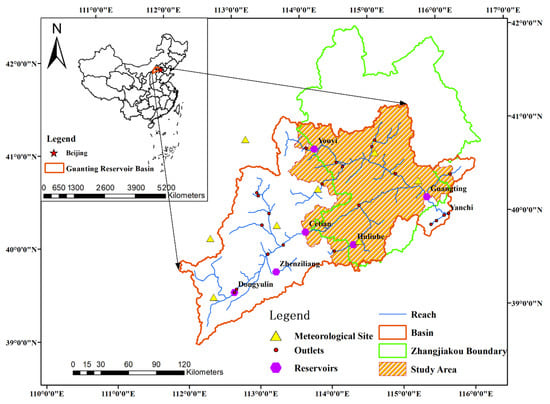
Figure 1.
Location of the Guanting Reservoir watershed and study area.
The input data of this study were meteorological, hydrological, statistical, and spatial. The spatial data included topographic data, land-use data, and soil-type data.
Meteorological data, which included the average temperature, precipitation, average wind speed, relative humidity, and sunshine hours, were obtained from the daily dataset of eight national meteorological stations provided by the National Meteorological Information Center (http://data.cma.cn, 14 February 2019). The stations’ location information is shown in Table 1. Hydrological data, which contained information about a total of 18 hydrological stations, were obtained from the Hydrological Yearbook of the People’s Republic of China. In addition, there are six reservoirs, namely the Dongyulin, Cetian, Zhenziliang, Huliuhe, Youyi, and Guanting Reservoirs. Reservoir information (surface area and volume when the reservoir is filled to the principal and emergency spillway, initial reservoir volume, initial sediment concentration, and the year the reservoir became operational) was added to the model according to the reservoir design index and the outflow data provided by the hydrological yearbook and Zhangjiakou water authority. Yanchi station, the nearest hydrological station downstream from Guanting Reservoir, was selected as the final outflow station, and the measured data were used to calibrate the water quantity and sediment yield. The measured ammonia and phosphorus data of the Bahaoqiao station, the water quality station nearest the Yanchi station, were used to calibrate the water quality data. The agricultural management data, containing irrigation and fertilizer application information, were provided by the Zhangjiakou Academy of Agricultural Sciences and were input into SWAT through the management module.

Table 1.
Location Information of Meteorological Stations, Reservoirs, Hydrological Stations, and Water Quality Stations.
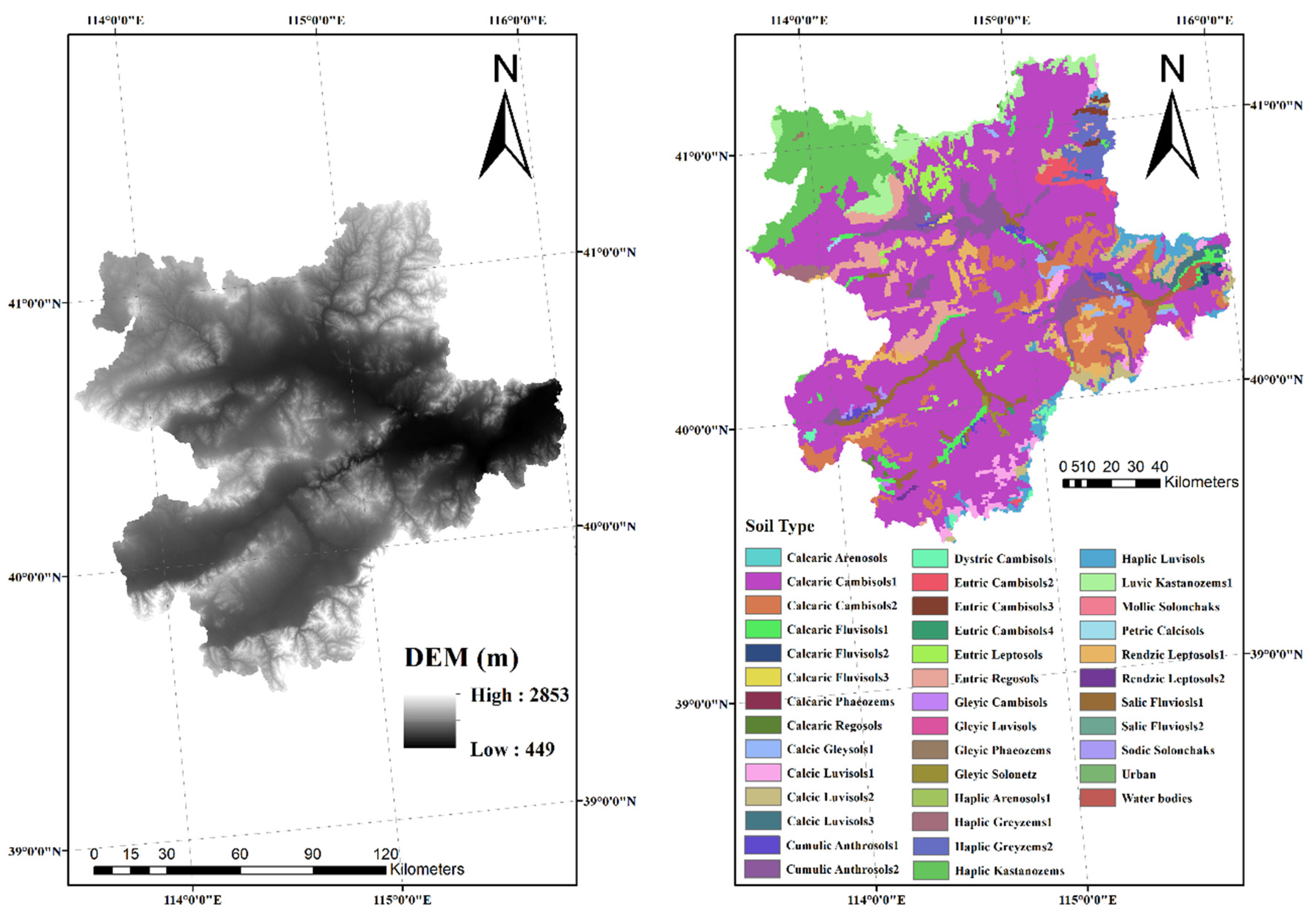
Topographic data were obtained from the Shuttle Radar Topography Mission (SRTM) 90 m resolution Digital Elevation Model (DEM) data (Figure 2) provided by the China Geospatial Data Cloud (http://www.gscloud.cn, 26 December 2018) and were used to generate river-network and subbasin boundaries within the watershed. Additionally, SWAT can overlay the river-network data on the DEM to assist in generating river channels, which can improve the hydrologic segmentation and depiction of subbasin boundaries when DEM data quality is not very good. The river-network data were obtained from the river-network dataset of Chinese watersheds provided by the Resource Environment Data Cloud (http://www.resdc.cn, 18 April 2019). Finally, SWAT generated 53 subbasins in the study area.
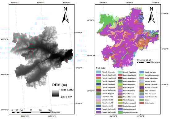
Figure 2.
DEM and distribution of soil types in the study area in 2016.
Soil data (Figure 2) were obtained from the Homogenized World Soil Database published by the Food and Agriculture Organization, which provides a global map of soil types at 1 km resolution and a database of the physical and chemical properties of different soil types.
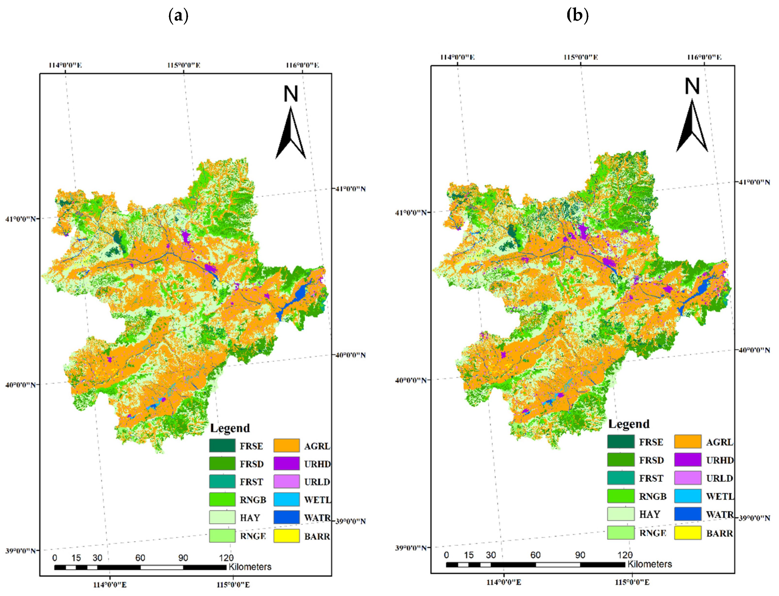
The land-use distribution was generated by China’s 1:250,000 land-cover data produced by the Aerospace Information Research Institute, the Chinese Academy of Sciences, and reclassified according to the SWAT land-use input code (Figure 3). After reclassification, it mainly includes six types of land use, namely forest, grassland, cropland, settlement, water body, and barren land. Under each type, there are several subtypes, among which, forest is divided into four types: evergreen forest (FRSE), deciduous forest (FRSD), mixed forest (FRST), and shrubland (RNGB). Grassland is further divided into grassland (HAY) and shrub grassland (RNGE); cropland (AGRL) is not divided into subtypes; settlement is divided into urban (URHD) and township (URLD); water body is divided into wetlands (WETL) and water (WATR); and barren land (BARR) is not divided into subtypes.

Figure 3.
The distribution of land-use types in the study area. (a): 2000, (b): 2016.
2.2. Assessment of Model Availability
In this study, the SWAT model was calibrated and validated in monthly steps. The warm-up period was set from 2008 to 2009, the calibration period from 2010 to 2013, and the validation period from 2014 to 2016. The Nash efficiency factor (NSE) [43], goodness of fit (R2), and percentage error (PBIAS) were used to evaluate the error introduced by the input data or the initial database of the model between simulated and observed values. The three indicators were calculated as follows:
where and are the observed and simulated values, respectively; and and are the average of the observed and simulated values, respectively. R2 describes the degree of deviation between the model simulation and the measured results. Its value is between 0 and 1, and a larger value indicates a better simulation; it is generally believed that a value of approximately 0.5 means an acceptable simulation result [44]. For the simulation of the monthly step size, when 0.75 < NSE ≤ 1, the fitting effect is very good; when 0.65 < NSE ≤ 0.75, the fitting effect is good; when 0.50 < NSE ≤ 0.65, the fitting effect is satisfactory; and when 0.50 ≤ NSE, the fitting is not acceptable [45]. PBIAS ≤ ±25% is acceptable [46].
Because the measured sediment output data of the Yanchi station during the study period were all zero, the parameters affecting sediment yield were calibrated along with the calibration of water quality data. SWAT considered the contribution of nutrients attached to the sediment when calculating the nutrients entering the river. When the simulation results of the nutrients met the requirements, we considered that the simulation results of the sediment were also acceptable.
2.3. Quantification of ESs
This study quantified different ESs using the SWAT model. The ESs covered a watershed-scale, a semi-distributed mechanistic model developed by the US Department of Agriculture, Agricultural Research Service, which was developed to predict the effects of different land management on water, sediment, and agrochemical yields in large, complex watersheds. The model decomposes watersheds into subbasins and hydrological response units (HRUs). Each HRU represents a unique combination of land use, soil type, and topographic slope to characterize the different ES quality outputs of plots with different hydrological characteristics.
2.3.1. WY and Water Conservation
The water balance method is used to calculate the water content. The difference between precipitation and evapotranspiration and surface runoff is considered the WC capacity [47,48]. The WY consists of three components: surface runoff, lateral flow, and baseflow [49].
where PCP is precipitation, ET is evapotranspiration, SURQ is the surface runoff, LATQ is the lateral flow, and GWQ is the baseflow; all components are measured in millimeters.
2.3.2. Soil Conservation
Erosion without human influence is called geologic erosion, and some human activities can increase the rate of erosion. Organic matter forms complexes with soil particles, so erosion of soil particles will also remove nutrients. Excessive erosion can deplete soil nitrogen and phosphorus needed for plant growth. Extreme erosion will degrade the soil function, and the soil will no longer sustain plant life. The erosion due to rainfall and runoff was calculated using the modified universal soil loss equation (MUSLE) [50].
where is the sediment yield in a given day (metric tons), is the surface runoff volume (mm H2O/ha), is the peak runoff rate (m3/s), is the area of the HRU (ha), is the universal soil loss equation (USLE) soil erodibility factor (0.013 metric ton m2 hr/(m3-metric ton cm)), is the USLE cover and management factor, is the USLE support practice factor, is the USLE topographic factor, and is the coarse fragment factor. After obtaining SY, its inverse was taken as the evaluation index of the SC capacity.
2.3.3. Nonpoint Pollution Control
The SWAT model assigns a different nutrient export to the river to different pathways; the main pathways include surface runoff, subsurface runoff, and sediment trapping. In this study, the total nitrogen and total phosphorus were calculated by summing the organic and inorganic nitrogen and phosphorus considered in SWAT, respectively. The calculation method is given as follows:
where (kg/ha) is the total nonpoint output of nitrogen;(kg/ha) is the organic nitrogen output; and (kg/ha), (kg/ha), and (kg/ha) are the NO3 entering the river through the surface runoff, lateral flow, and baseflow, respectively. is the ammonia nitrogen content entering the river with the surface runoff. is the total nonpoint output of phosphorus, (kg/ha) is the organic phosphorus output, (kg/ha) is the amount of inorganic phosphorus that enters the river with the surface runoff, and (kg/ha) is the inorganic phosphorus attached to the sediment. After obtaining the total nitrogen and phosphorus yields, their inverse values were taken as the evaluation indices of nitrogen (NF) and phosphorus fixation (PF) capacities, respectively.
2.3.4. Soil Carbon
The SWAT carbon submodule mainly considers the contribution of soil organic matter and litters to soil carbon. Based on the conceptual description of the soil carbon model of previous studies [51], SWAT calculates soil carbon as follows:
where is soil carbon (kg/ha), is the rate of humification (kg/kg), is the contribution of litters (kg/m2) provided by the crop database in SWAT, is the apparent turnover rate of soil organic matter provided by the HRU database in SWAT, is saturation soil organic carbon mass (kg/ha), clay is the proportion of soil clay content. The obtained soil carbon content is used as an evaluation index of carbon sequestration capacity (CF). SWAT only describes the stable carbon pool, and there might be some differences between the simulation results and the real situation, but it can still be used for trend analysis.
2.4. Quantitative Analysis of ESs Relationships
The implementation of ecological projects reflects the human pursuit of different goals in practice, usually changing regional land-use types. It is a subjective driving force that affects the changes of various resources in the region. Afforestation is a common ecological project for improving the regional ecological environment.
2.4.1. Quantitative Expression of ES Relationships and Intensity
Different ESs were calculated in the 53 subbasins. The ESs were normalized to identify the relationships between these different ESs before the Spearman correlation analysis.
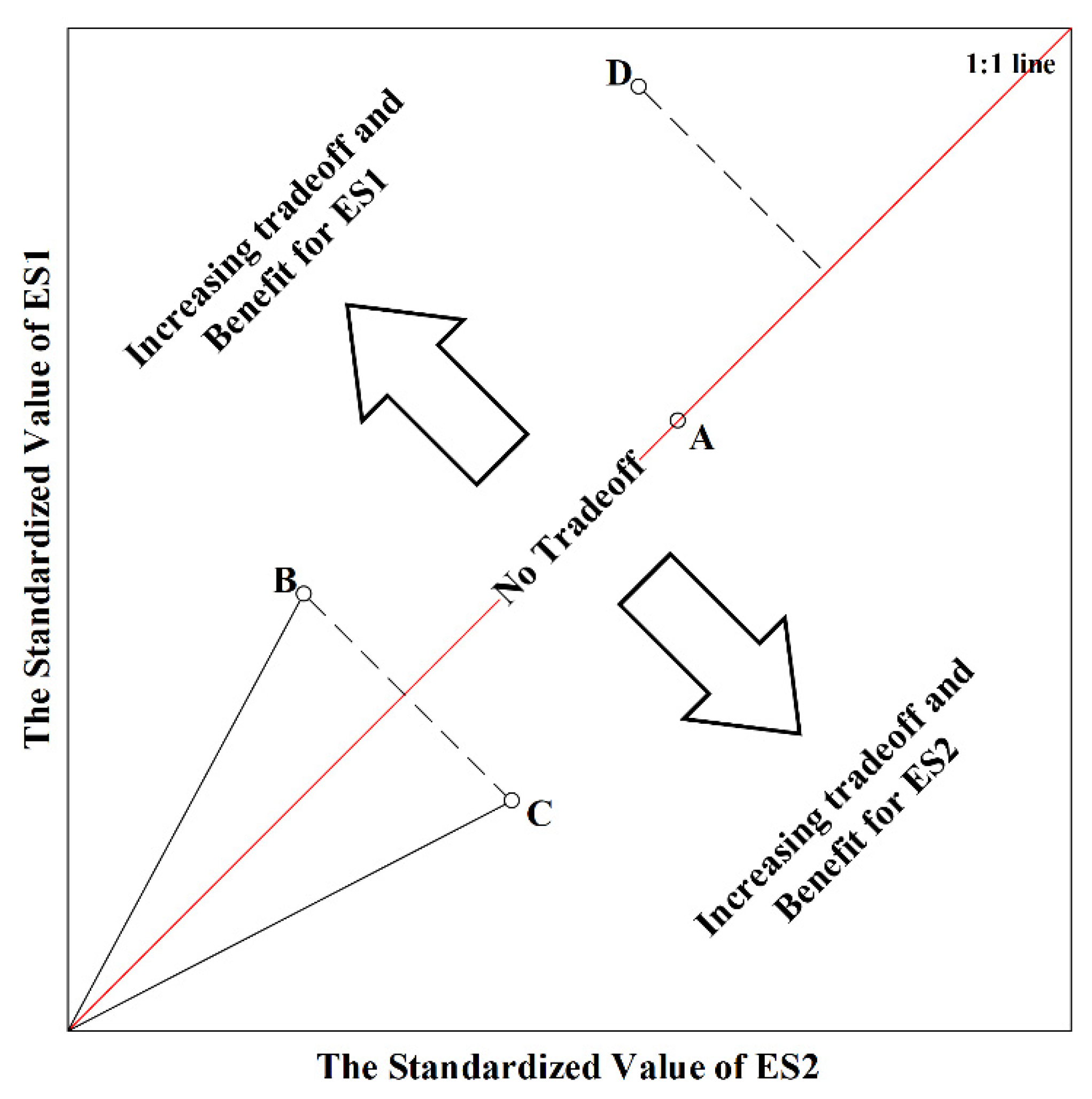
The intensity of the ES trade-off relationship was measured using the root mean square error (RMSE) [19,52,53,54]. Mathematically, RMSE is the distance from the coordinates of a pair of ESs to the 1:1 line. The 1:1 line in two dimensions indicates that there is no tradeoff between the two ESs. The further away the coordinates from the line, the stronger the tradeoff. The RMSE indicates the average distance between all the points and the line (Figure 4). The calculation formula is given as follows:
where represents the standardized value of any ES, and , , and represent the simulated value of the ES, and the minimum and maximum of the simulated values, respectively; Tr is trade-off intensity. is the standardized value of ES i, and is the expected value of several ESs.
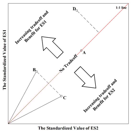
Figure 4.
Quantitative expression of the trade-off intensity between two ESs. There is no tradeoff between the two ecosystems at point A. The tradeoff is stronger at point D than those at points B and C. The equal distance between points B and C and the 1:1 line indicates that the trade-off intensity is the same at both points, but B is more beneficial to ES1, and C is more beneficial to ES2. This figure was adapted from a previous study [54].
Different land-use types are located in different spatial locations which have different precipitation. Different precipitation will lead to changes in water-related ecosystem services, and the introduction of a new variable will compromise the study of ecosystem service response to land-use change. To eliminate the effect of the difference in the spatial distribution of precipitation, all ESs mentioned above were divided by precipitation.
2.4.2. Analysis of Factors Influencing ESs Relationships
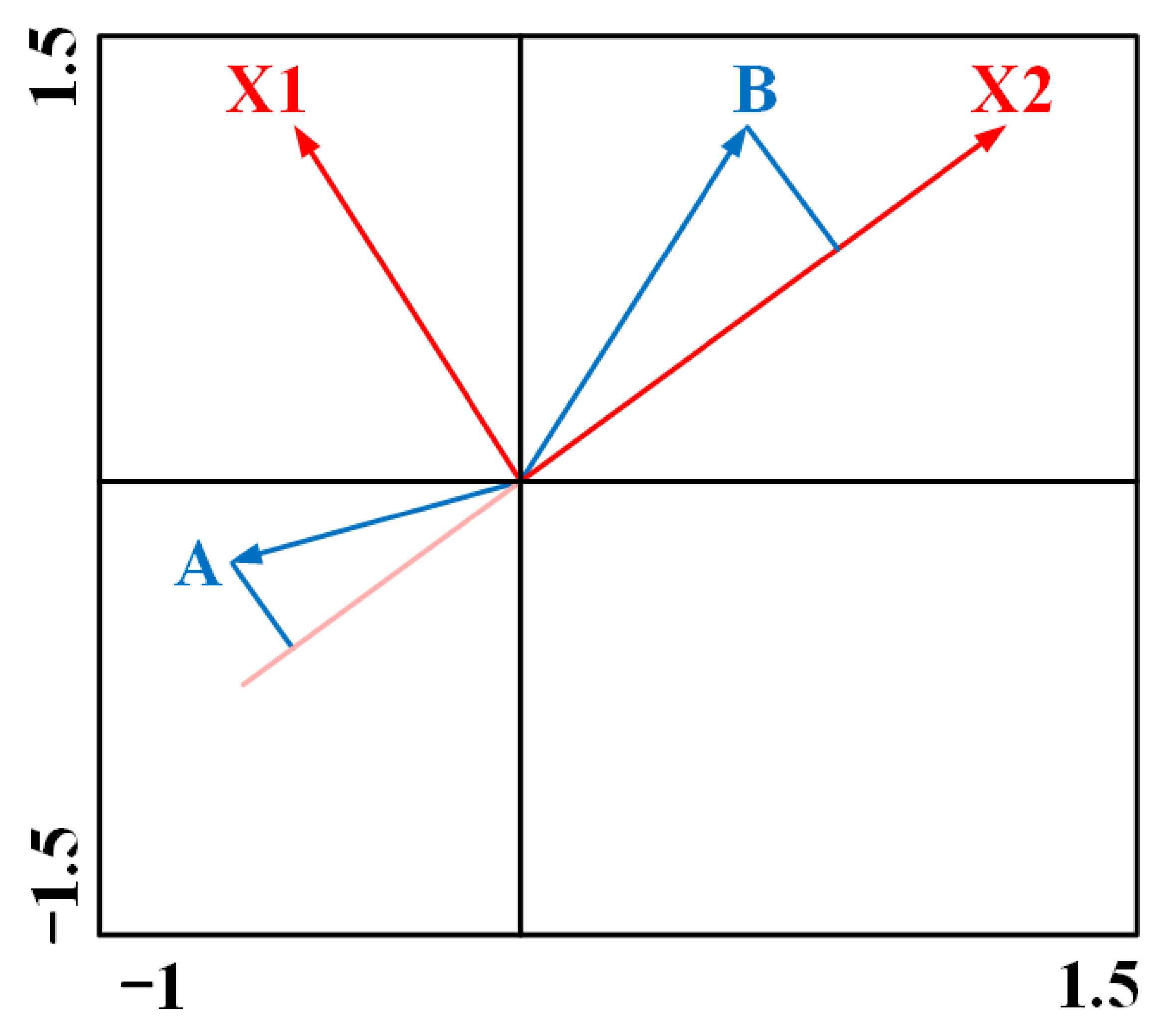
A multivariate analysis was applied to explore the impact of land-use change on changes in ESs due to the implementation of afforestation. A detrended correspondence analysis (DCA) was performed to determine whether a linear or unimodal numerical approach should be used. In this study, the maximum DCA gradient length value was shorter than 3.0, which indicates a linear approach is more rational [41]. Therefore, the relationships between the variables were analyzed using redundancy analysis (RDA), with the percentage changes in land-use area (environmental factors), change in trade-off intensity, and the corresponding percentage change in ESs (species factor) in different subbasins as input data. Monte Carlo permutation tests based on 499 random permutations were conducted to test the significance of the eigenvalues of all canonical axes and the significance of marginal and conditional effects. The effect of the explanatory variables on the response variables was evaluated by conditional and marginal effects, with higher values indicating a stronger effect [19]. The marginal effect reflects a degree of influence of environmental factors on ESs, and the conditional effect reflects the degree of influence of the current environmental factor on ESs after removing the previous environmental factor [41]. The example graphical result of the RDA analysis is shown in Figure 5.
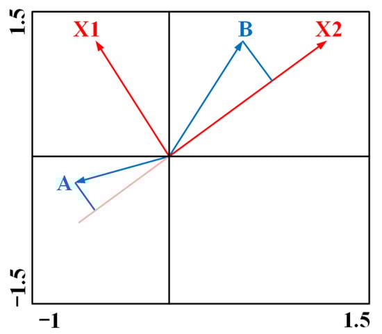
Figure 5.
Biplot of RDA. We can approximate the correlation between the response variables (A,B) and an explanatory variable (X2) by a perpendicular projection of the species arrow tips (A,B) onto the line overlaying the environmental variable arrow (X2). The further a projection point falls in the direction indicated by the arrow, the higher the correlation, with a projection point near the coordinate origin (zero point) suggesting no correlation. If the projection point lies in the opposite direction (A), the predicted correlation is negative. A similar, but less precise interpretation can be based on the angle between the two compared arrows. The statistics were carried out using the R vegan packages.
3. Results
3.1. Validation of SWAT
The parameters related to different hydrological processes were selected from the SWAT input/output documentation for sensitivity analysis. Sensitive parameters were determined using global sensitivity analysis and one-at-a-time sensitivity analysis in SWAT-–CUP. The optimized ranges of sensitive parameters were automatically calibrated by the SUFI-2 algorithm in SWAT–CUP, and the most fitted parameter values are shown in Table 2.
Table 2.
Optimal Parameter Values After Calibration.
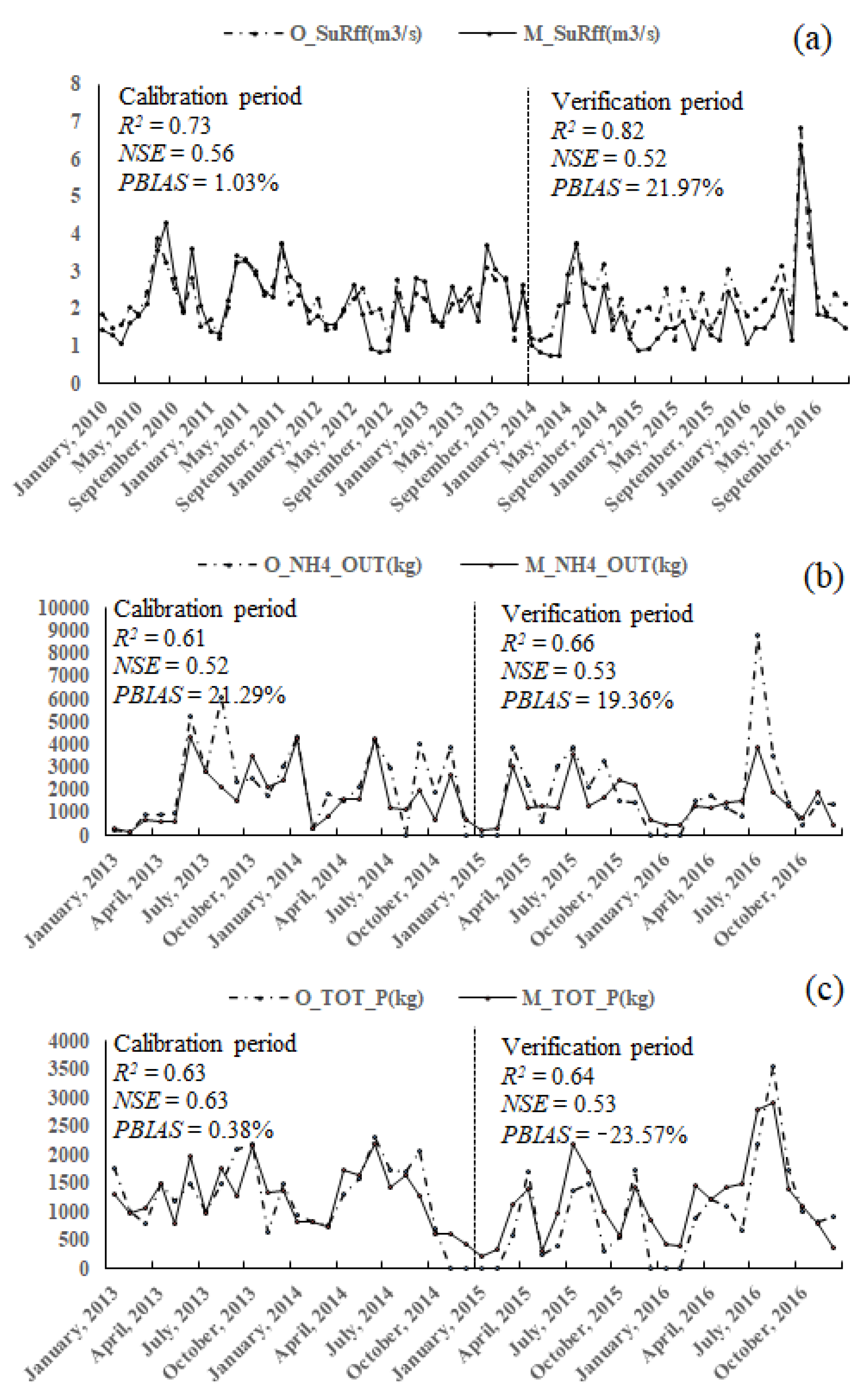
The calibrated model performed well (Figure 6); the monthly simulation result is available. NSE were all higher than 0.5, R2 were all higher than 0.6, and PBIAS were all less than 25%. The SWAT model built in this study is applicable to simulating the hydrologically related process in the Zhangjiakou section of the Guanting Reservoir basin.
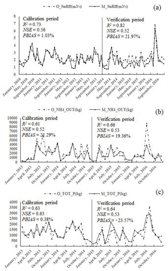
Figure 6.
Simulation results of monthly runoff (a), ammonia (b), and total phosphorus (c). SuRff, NH4_OUT and NH4_OUT demotes monthly outputs of runoff, ammonia, and total phosphorus, and the letters O and M denote observed and simulated values, respectively. R2, NSE, and PBIAS denote goodness of fit, Nash efficiency factor, and percentage error, respectively.
3.2. Land Use and ESs Changes under Afforestation
The interconversion between the different land-use subclasses and the amount of net change in the conversion process is shown in Figure 7. Forest area increased the most, with grassland contributing the most, followed by cropland. Grassland had the most area converted to evergreen forests, and cropland had the most area converted to deciduous forests. Except for the conversion to forest, the largest area of grassland was converted to settlement, but the largest contribution to the increase in settlement was made by cropland. The growth rate of urban area (144.97%) follows that of forest, with a small increase in township area (1.39%). The overall percentage of settlement area was low.
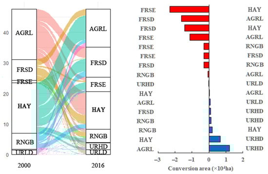
Figure 7.
Land-use subclass conversions in the study area from 2000 to 2016. The right panel shows the net subclass conversions; only 16 change patterns with change areas greater than 100 ha are shown in the figure. Positive and negative values indicate the direction of land-use conversion. AGRL, FRSD, FRSE, HAY, RNGB, URHD, and URLD denote cropland, deciduous forest, evergreen forest, grassland, shrubland, urban, and township, respectively. The structure of land-use percentage has changed (Figure 8). The area of land use other than water bodies and barrens covered more than 97% of the entire study area. Land uses are mainly dominated by croplands, and the other types in descending order of area are grassland, forest, shrub, and settlement. The area of grassland, cropland, and shrub decreased by 1.97%, 1.86%, and 0.41%, respectively, in 2016 compared with 2000. The land use that increased in the area was forest and settlement, which increased by 3.32% and 1.04%, respectively.
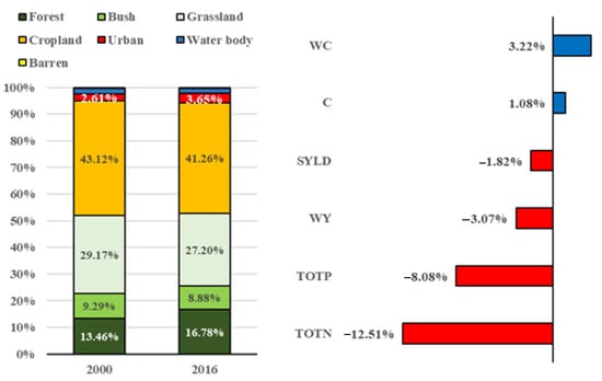
Figure 8.
Land-use change from 2000 to 2016. The left panel shows the percentages of different land-use classes in 2000 and 2016. The right graph shows the change rate of different ESs.
Figure 8.
Land-use change from 2000 to 2016. The left panel shows the percentages of different land-use classes in 2000 and 2016. The right graph shows the change rate of different ESs.

Along with land-use change, different ESs have also changed. The amount of water content and soil organic carbon content increased, with a 3.22% increase in water content, and 1.08% in soil carbon content. WY, sediment yield, total nitrogen output, and total phosphorus output decreased, and the largest decrease occurred in total nitrogen output (–12.51%). The process of mutual transformation of land uses is complex, and the general trend of change is the transformation of different land-use types to evergreen forests and urban areas. Afforestation and urbanization processes have a great impact on regional land use and various ESs. Because the area of forest, shrubland, grassland, cropland, and wetland accounts for more than 95% of the total study area, the following sections focus on these five land-use types and their subclasses.
3.3. ESs Relationships and Their Linkages with Land-Use Changes
3.3.1. Analysis of Relationships between ESs
As shown in Table 3, WY had a trade-off relationship with WC, SC, NF, and PF, whereas WC, SC, NF, and PF had synergistic relationships with each other (Table 2). NF and PF had a significant synergistic relationship with each other, and both of them had significant trade-off relationships with WY and synergistic relationships with SC. NF had a stronger relationship with WY, while PF had a stronger relationship with SC since most of the phosphorus in the soil appeared insoluble and is mostly lost with soil erosion [55]. CF had nonsignificant relationships with the other ESs.
Table 3.
Change Matrix of the Spearman Correlation Coefficient between Different ESs from 2000 to 2016.
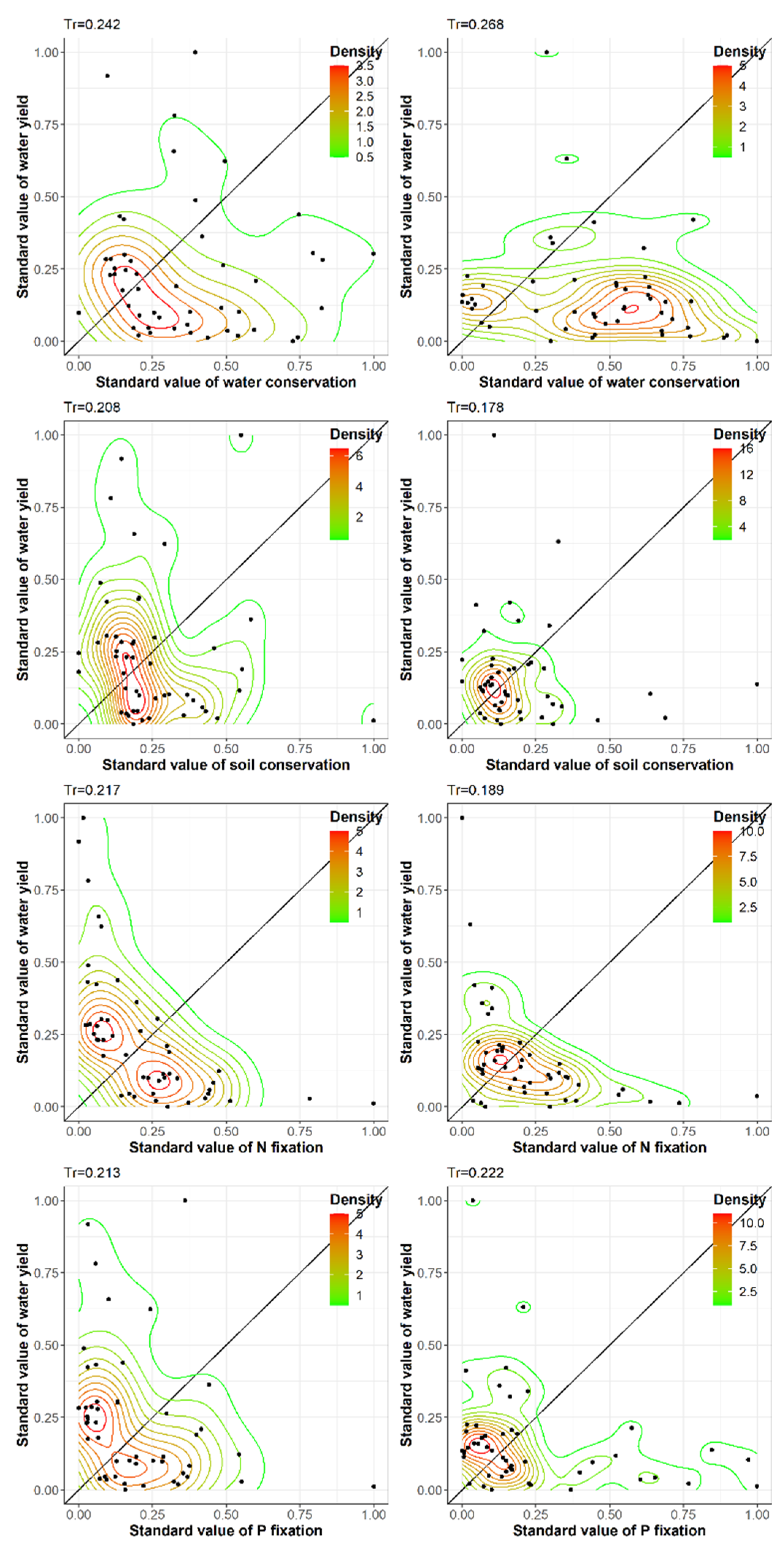
Strong tradeoffs between ESs will encumber the development of multi-ES synergies. We then focused on ES pairs that have significant tradeoffs to see how they changed. The tradeoff between WY and WC is the strongest, the WY–SC tradeoff is the weakest, and the trade-off intensities of WY–NF and WY–PF were similar (Figure 9). The WC–WY trade-off intensity (Tr) became stronger, and more points were distributed below the 1:1 line, indicating that the afforestation projects had largely promoted the ability of WC in Zhangjiakou City; however, this has weakened the capacity of the water supply downstream. The WY–SC trade-off intensity changed from 0.208 to 0.178, meaning that there was a more balanced relationship between WY and SC. The points on the plots showing relationships of NF and PF with WY tended to be more clustered in the NF and PF sides in 2016 compared with 2000, indicating that land-use changes in Zhangjiakou had more benefited the NF fixation and PF fixation than the WY.
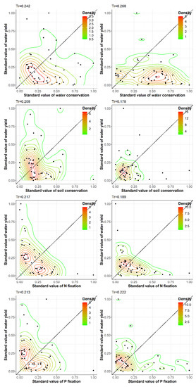
Figure 9.
ESs trade-off intensity of 2000 (left column) and 2016 (right column). Tr indicates trade-off intensity. The area with dense contours has dense point distribution, and the overall trend of point distribution can be identified by the change of contour distribution.
3.3.2. Impact of Land-Use Change on ESs Change
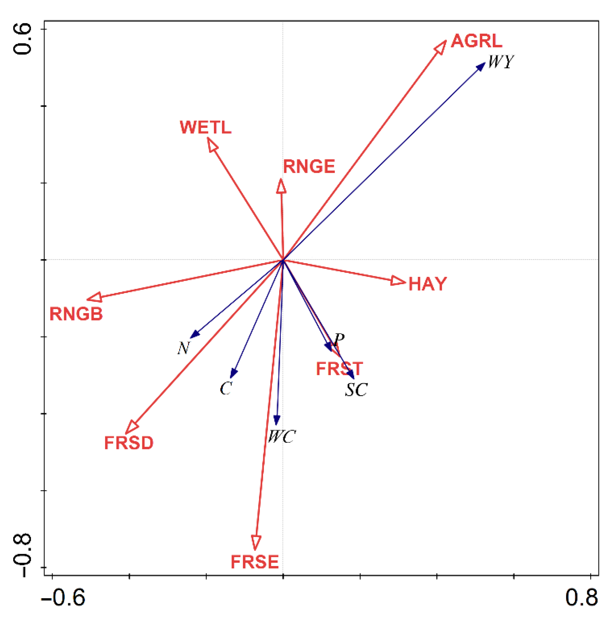
RDA was performed to analyze the contribution of different land-use changes to various ES changes. As shown in Table 4, the canonical relationship was significant (p < 0.01), with a cumulative explanation of 20.15% for the first two axes of the RDA, which means that RDA is capable of explaining the role of land-use change in the change of ESs. Biplot results are shown in Figure 10.
Table 4.
Eigenvalues and Explained Variance of the RDA Axes for the ESs.
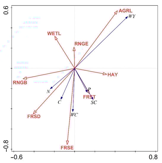
Figure 10.
Biplot diagram for the RDA between the ESs and land uses.
Table 5 shows the marginal and conditional effects generated by the Monte Carlo test for the environmental factors in the forward selection process. Most of the conditional effects were insignificant, indicating that there were interactive effects of different environmental factors on the ESs. The land-use effects on each ES are listed in Table 5.
Table 5.
Marginal and Conditional Effects from the Summary of Forward Selection for Different ESs.
As shown in Figure 10 and Table 5, forest, shrubland, and grassland with a good canopy structure contributed to various ESs. The soils under FRSE have high soil porosity, and the water infiltration rate is fast [56,57], which gives FRSE a strong WC capacity. Canopy retention reduces some of the precipitation reaching the ground [58], thus reducing WY. With the decrease in WY, the loss of nitrogen and phosphorus with runoff decreases [59]; thus, FRSE contributes to NF and PF. FRSD’s canopy is more depressed and will trap more precipitation [14,60]. Thus, FRSD can significantly reduce WY, and the smaller capillary porosity of the understory soil [57] makes FRSD less capable of conserving water than FRSE. However, easily decomposed litter will provide more carbon accumulation in FRSD understory soil [61,62], which gives FRSD a strong CF capability. Most of the nitrogen is lost with runoff [63]; FRSD reduces water yield, the main carrier of nitrogen, so it has good NF capability. A higher soil aggregate retention rate and clay content provide higher water stability of the soil under FRST [61], resulting in a superior SC capacity. Most phosphorus attaches to the soil and is lost with runoff [55], and reduction in soil loss has led to lower phosphorus loss, resulting in a good PF capacity of FRST.
RNGB is vegetation having a similar structure to forests [64], but its canopy structure is not as rich as that of the forest [65]; its ability to decrease WY and increase CF is weaker. The contribution of RNGE to all of the ESs was not significant. Grasslands are rich in roots [66], enabling them to provide multiple ESs. However, the soil physical and chemical properties of grassland substrates, such as higher soil density [67,68] and less litter [64], result in a smaller contribution to ESs. The relatively simple canopy structure of AGRL makes its canopy-retention capacity poorer than that of trees and shrubs, so that more precipitation will fall to the ground, thus increasing the water yield. In addition, more precipitation falling directly onto the soil has weakened the erosion resistance of cropland soils and reduced field water content, humus, and organic matter content [69]. Ultimately, the soil carbon content decreases, and the amount of flow production and soil loss increases, coupled with the application of chemical fertilizers, causing a serious loss of nitrogen and phosphorus. Although WETL can enhance soil and WC capacity, the capacity is weaker than that of other land uses [67]. When its area is transferred to other land uses or reverse conversion occurs, soil and water conservation capacity will be enhanced and reduced, respectively, indicating that the change in WETL area and the change in soil and water conservation capacity are negatively correlated.
Generally speaking, vegetation types with rich canopy structures can effectively reduce WY by intercepting a significant portion of precipitation when it occurs [14]. By contrast, bare soil under vegetation with a relatively simple structure will be directly eroded by precipitation and runoff [17], which results in a weaker SC, and this will increase the risk of nitrogen and phosphorous diffusion with runoff and sediment.
3.3.3. Impact of Land-Use Change on Change of Relationship between ESs
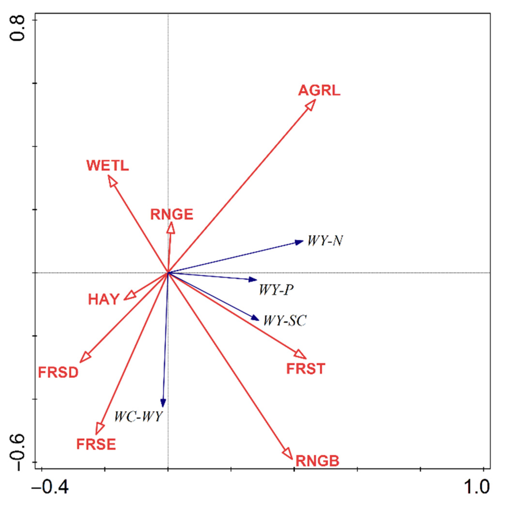
ESs are related to each other, and afforestation affects ESs by changing land use, which in turn affects tradeoffs. The effect of land-use change on trade-off intensity was evaluated by marginal and conditional effects. As shown in Table 6, the canonical relationship was significant, with a cumulative explanation of 23.34% for the first two axes of RDA, which means that RDA is capable of explaining the role of land-use change in the change of ES tradeoff intensities. Biplot results are shown in Figure 11.
Table 6.
Eigenvalues and Explained Variance of the RDA Axes for Various Tradeoffs.
Figure 11.
Biplot diagram of the RDA between various tradeoffs and environmental factors.
Table 7 shows the marginal and conditional effects generated by the Monte Carlo test for the environmental factors in the forward selection process. As shown in Table 7, there are markedly more environmental factors with significant marginal effects than with significant conditional effects, indicating a strong interactive effect of environmental factors on ESs tradeoffs. The land-use effects on ESs relationships are presented in Table 7.
Table 7.
Marginal and Conditional Effects from the Summary of Forward Selection for Different ES Tradeoffs.
The difference in the contribution of different ecosystem types to the ESs will affect the relationship between ESs. For example, in a WC–WY tradeoff, AGRL can reduce the extent of the tradeoff. Although it tends to increase WY, the difference between the degree of favoring WY and favoring WC is smaller. RNGB, FRSD, and FRSE will increase the extent of the tradeoff. FRSD and RNGB have a strong ability to reduce WY, and FRSE is the largest contributor to WC increase; the ranking of increasing capacities is FRSE > RNGB > FRSD. A comparison of Table 4 and Table 6 shows that tradeoffs arise between various ecosystem types although all ecosystem types can enhance one or more ESs. It is remarkable that HAY has a weaker contribution to the improvement of ESs, but fewer tradeoffs occur with the increase in HAY area, which implies that HAY can enhance ESs without weakening other ESs.
A combination analysis with Figure 9 reveals that changes in ESs and their relationships are associated with changes in land use, which are led by afforestation projects in the study area. The decrease in AGRL and increase in FRSE were responsible for the exacerbation in the WY–WC tradeoff. The decrease in FRST and increase in WETL weakened the WY–SC tradeoff. The weakened WY–NF tradeoff was caused by the combined effects of the reduced AGRL and RNGB and increased FRSE, FIRST, and AGRL, which exacerbated the WY–PF tradeoff. HAY, which mitigated the WY–PF tradeoff, were simultaneously reduced, resulting in the exacerbation of the WY–PF tradeoff.
4. Discussion
Afforestation is a powerful anthropogenic intervention, adjusting and rearranging land management practices. It aims to achieve sustainable development by changing regional land use and is widely implemented in several countries around the world. Studies have shown that afforestation improves ecosystem regulation services and the quality of local ecosystems [29,70]. However, some studies have also found that the tradeoff between provision and regulatory services will become increasingly evident with the implementation of GFGP [71,72].
Therefore, the complexity of the trade-off relationships between ESs under afforestation projects needs to be considered to understand the integrated benefits of afforestation, which is critical for promoting the sustainable development of services in each ecosystem. In terms of synergies and tradeoffs between ESs, the tradeoff between WY and other ESs is one of the challenges that constrain sustainable development [73]. When tradeoffs are unavoidable, the selective change in land-usage strategies according to regional ecological development requirements is an effective way to maximize ecological benefits.
The results of this study are very similar to those of previous researchers in terms of ESs and their interrelationships. For example, in Yunnan, which is located in the tropical monsoon climate zone of southwest China, the GFGP also enhanced the local carbon sequestration and water conservation functions by 3.49% and 0.83%, respectively, while decreasing the water yield by 0.83% [18]. In Shandong province, which is located in a temperate monsoon climate zone in eastern China, studies have shown that the GFGP can significantly improve the control of nonpoint source pollution [74]. Another study in Yunnan Province showed that the GFGP would effectively contribute to the enhancement of soil retention, but at the cost of a decrease in streamflow production [29]. Water yield in Nanjing, located in the subtropical monsoon zone, increased by 33.03% from 2005 to 2010, while carbon sequestration and soil conservation decreased by 0.75% and 7.75%, respectively, forming a trade-off relationship between these ESs [73]. An assessment of ESs in southern China using the InVEST model found a significant synergistic relationship between water yield and nitrogen and phosphorus export, suggesting a trade-off between water yield and pollution diffusion control [75]. In the Heihe River Basin, which is located in a temperate continental climate zone in northwest China, synergy between water conservation, soil conservation, pollution control, and carbon sequestration is a dominant relationship [66]. A study in the YLN basin (the basin of Yarlung Tsangpo River, Lhasa River, and Nianchu River) in Tibet, which is located in a mountain plateau climate zone, indicated a significant synergistic relationship between water conservation and both carbon sequestration and soil conservation [76]. Most of the characteristics of ESs and the relationships between them were the same as those obtained in previous studies in different climate zones. The synergistic WC–SC relationship observed in 2016 differs from some previous conclusions [77], but it has also been pointed out that the implementation of ecological projects changes the WC–SC tradeoff relationship [77,78]. The implementation of afforestation projects in the study area enhanced both WC and SC, making the relationship between them develop in a synergistic direction.
Over a long period of time, the characteristics of changes in ESs and their relationships are similar to this study, while the main influencing factors of these changes evolved significantly. In the analysis of the relationship between flow production, water purification, soil conservation, carbon sequestration, and habitat quality in the South Four Lakes Basin of Shandong Province from 1980 to 2018, it was found that, with the increasing area of land for construction in economic development, the water yield is becoming stronger and flood risk is increasing; the strength and direction of ESs relationships change over time, and the trade-off between water yield and water purification is always the most obvious and exacerbating [79]. In terms of changes in the relationship between supply and regulating services in each administrative region in the Greater Bay Area from 2000–2015, the overall relationship is dominated by synergies with varying degrees, and it is accompanied by the occurrence of trade-off relationships of varying degrees [80]. Analysis of the factors influencing ES changes in the Heihe River Basin from 1980–2010 found that climate change factors on larger time scales had a more significant impact on water-related ESs than land-use changes [81].The contribution of different land uses to ESs was different. Land uses with a good canopy structure can effectively improve the regional ecological environment but may also result in more drastic tradeoffs. In the study area, FRSE exacerbated the WC–WY tradeoff because of a relatively weak negative effect on WY and a strong positive effect on WC. Compared with other land uses, FRSE is more suitable for planting in areas where WC and NF fixation are needed. FRSD has an average WC capacity, but it can enhance CF and reduce WY, and planting FRSD is a good choice when runoff regulation and carbon fixing are needed. The contribution of FRST to different ESs is quite different [41], which leads to multiple tradeoffs. Considering the coordinated development of the ecological environment, FRST is not suitable in areas with similar climatic conditions and topographical features as the study area. In terms of water retention, soil sequestration, and nitrogen and phosphorus diffusion control, RNGB and FRSE have similar tradeoff characteristics, but RNGB has a smaller contribution [64,82]. RNGE does not contribute significantly to any ES or tradeoff compared with other land-use types in the study area. Some studies have pointed out that shrubs can make a prominent contribution to soil organic carbon accumulation. Studies suggested that soil carbon accumulation is affected by soil type. In soils with a high sand content, trees are more conducive to organic carbon accumulation. By contrast, shrubs are more likely to accumulate organic carbon in soils with more silty clay particles and agglomerates [64]; 10.09% of the shrubs in the study area were planted in areas with a high soil sand content, which may be the reason for the shrubs not fully performing their ecological functions. Conversion of shrubs planted on sandy soil to other land uses can be considered when afforestation is carried out to improve ESs. HAY contributes to all ESs except CF and NF. Because of its weaker capacity of enhancing CF and NF, with the constant study area, an increase in the HAY area leads to a relative weakening of ESs. Meanwhile, HAY exacerbates the weakest tradeoffs [19]. HAY can enhance multiple ESs without exacerbating too many tradeoffs; considering the integrated development of regional ecosystems, partially changing land use that deteriorates the tradeoffs to HAY may be an effective method to maintain ESs while preventing overconsumption of other ESs. The specific ecological problems and corresponding solutions are shown in Table 8.
Table 8.
Solutions for Different Ecological Problems and the Scenarios under Different Restoring Scheme Strengths Consisting of Different Solutions.
Soil pH affects soil fertility; intense nitrogen deposition is the main reason for soil acidification, and land-use-type conversion is the main factor affecting soil properties [83,84]. While studying the control of nitrogen and phosphorus surface source pollution by land-use policies, it is also necessary to extend the focus to the nitrogen and phosphorus content in soils to form a theoretical support for future land-health-restoration strategies. The influencing factors of different ESs vary at different spatial scales; human activities are more likely to affect ESs at small scales. At larger scales, the influence of environmental factors are dominant [85]. Similarly, the factors influencing ES relationships differ across time scales; long-term ES changes are more sensitive to climatic elements. This study checked changes in meteorological factors, resulting in a relatively low cumulative explained variation of the RDA. Water-related ESs are highly sensitive to precipitation and temperature [41], and meteorological elements should be considered in future studies to further complete the analysis of factors influencing ESs. The change patterns of ESs with time are becoming clear, and the next step is to analyze the ESs and their interrelationships at different time intervals to find the time scales that are sensitive to changes in ESs and their relationships, which can help in formulating a more comprehensive land-use strategy under the goal of the sustainable development of ESs. Moreover, the effects of environmental factors on tradeoffs can be statistically described by RDA, but individual ESs are influenced by multiple land uses, and each land use affects multiple ESs. Besides, ESs are not isolated from each other, and relationships that exist between ESs will blur the judgment of factors influencing ESs relationships [8]. The response mechanism of ESs and their changes to land-use changes needs to be further studied.
5. Conclusions
In this study, we quantified four ESs (water yield, water and soil conservation, nonpoint pollution control, and soil carbon sequestration) of Zhangjiakou in the Guanting Reservoir basin by the SWAT model. Changes in different ESs and the tradeoffs between them were analyzed; then, we further analyzed the response of changes in tradeoffs to land-use changes caused by afforestation projects. The afforestation project changed ESs and relationships between ESs by changing land uses. With changes of land use, water conservation and soil carbon content have increased, whereas those of WY, sediment yield, nitrogen and phosphorus loss have decreased. The regional ecological environment has improved. Significant tradeoffs occur between WY and other ESs, except soil carbon sequestration. The intensity of the tradeoffs has changed. Tradeoffs between WC and WY, and phosphorus loss control and WY were exacerbated, whereas tradeoffs between SC and WY, and nitrogen and WY were mitigated.
Several ESs have been enhanced at the cost of WY in the study area. When tradeoffs cannot be avoided, we should focus on ESs that need to be enhanced urgently and bring forward a corresponding land-use planning scheme by selecting one or several land-use combinations under the premise of causing no excessive losses of other ESs. Mixed forest has the function of SC and phosphorus loss control, but it exacerbates too many tradeoffs, so mixed forest not a suitable afforestation species from the perspective of ecological sustainable development. Planting evergreen forest is not only an effective way to enhance WC, but it also benefits nitrogen loss control. Planting a deciduous forest can control WY and enhance soil carbon sequestration. Grasslands contribute to multiple ESs and do not excessively exacerbate tradeoffs. Replacing land-use types with strong tradeoffs with grassland can help achieve a synergistic development of ESs.
Author Contributions
Conceptualization, T.P.; methodology, T.P.; software, T.P.; formal analysis, T.P.; data curation, T.P. and Y.L.; writing—original draft, T.P.; writing—review & editing, L.Z., F.S. and Z.Z. (Zijuan Zhu); visualization, T.P.; validation, L.Z.; supervision, L.Z., Z.Z. (Zengxiang Zhang), X.Z. and F.S.; funding acquisition, L.Z.; project administration, Z.Z. (Zengxiang Zhang) and X.Z. All authors have read and agreed to the published version of the manuscript.
Funding
This work was funded by China’s Major Science and Technology Program for Water Pollution Control and Treatment, grantnumber 2017ZX07101001005 and the Aerospace Information Research Institute, Chinese Academy of Sciences, grant number Y8Q0050036.
Institutional Review Board Statement
Not applicable.
Informed Consent Statement
Not applicable.
Data Availability Statement
The data used to support the findings of this study are available from the corresponding author upon request.
Conflicts of Interest
The authors declare no conflict of interest.
References
- Costanza, R.; d’Arge, R.; de Groot, R.; Farber, S.; Grasso, M.; Hannon, B.; Limburg, K.; Naeem, S.; O’Neill, R.V.; Paruelo, J.; et al. The value of the world’s ecosystem services and natural capital. Ecol. Econ. 1998, 25, 3–15. [Google Scholar] [CrossRef]
- Khosravi Mashizi, A.; Sharafatmandrad, M. Assessing ecological success and social acceptance of protected areas in semiarid ecosystems: A socio-ecological case study of Khabr National Park, Iran. J. Nat. Conserv. 2020, 57, 125898. [Google Scholar] [CrossRef]
- Li, S.; Zhang, C.; Liu, J.; Zhu, W.; Ma, C.; Wang, J. The tradeoffs and synergies of ecosystem services: Research progress, development trend, and themes of geography. Geogr. Res. 2013, 32, 1379–1390. [Google Scholar]
- Douglas, I. Ecosystems and Human Well-Being; Island Press: Washington, DC, USA, 2017; Volume 1–5, ISBN 9780128096659. [Google Scholar]
- Bennett, E.M.; Peterson, G.D.; Gordon, L.J. Understanding relationships among multiple ecosystem services. Ecol. Lett. 2009, 12, 1394–1404. [Google Scholar] [CrossRef] [PubMed]
- Raudsepp-Hearne, C.; Peterson, G.D.; Bennett, E.M. Ecosystem service bundles for analyzing tradeoffs in diverse landscapes. Proc. Natl. Acad. Sci. USA 2010, 107, 5242–5247. [Google Scholar] [CrossRef] [Green Version]
- Haase, D.; Schwarz, N.; Strohbach, M.; Kroll, F.; Seppelt, R. Synergies, trade-offs, and losses of ecosystem services in urban regions: An integrated multiscale framework applied to the leipzig-halle region, Germany. Ecol. Soc. 2012, 17, 1–22. [Google Scholar] [CrossRef]
- Rodriguez, R.P.; Beard, T.D.; Bennet, E.M.; Cumming, G.S.; Cork, S.J.; Agard, J.; Dobson, A.P.; Peterson, G.D. Trade-offs across Space, Time, and Ecosystem Services. Ecol. Soc. 2006, 11, 1–14. [Google Scholar] [CrossRef] [Green Version]
- Wu, J. Landscape sustainability science: Ecosystem services and human well-being in changing landscapes. Landsc. Ecol. 2013, 28, 999–1023. [Google Scholar] [CrossRef]
- Posner, S.M.; McKenzie, E.; Ricketts, T.H. Policy impacts of ecosystem services knowledge. Proc. Natl. Acad. Sci. USA 2016, 113, 1760–1765. [Google Scholar] [CrossRef] [Green Version]
- Bryan, B.A.; Gao, L.; Ye, Y.; Sun, X.; Connor, J.D.; Crossman, N.D.; Stafford-Smith, M.; Wu, J.; He, C.; Yu, D.; et al. China’s response to a national land-system sustainability emergency. Nature 2018, 559, 193–204. [Google Scholar] [CrossRef]
- Chen, C.; Park, T.; Wang, X.; Piao, S.; Xu, B.; Chaturvedi, R.K.; Fuchs, R.; Brovkin, V.; Ciais, P.; Fensholt, R.; et al. China and India lead in greening of the world through land-use management. Nat. Sustain. 2019, 2, 122–129. [Google Scholar] [CrossRef]
- Dechmi, F.; Burguete, J.; Skhiri, A. SWAT application in intensive irrigation systems: Model modification, calibration and validation. J. Hydrol. 2012, 470–471, 227–238. [Google Scholar] [CrossRef] [Green Version]
- Jia, X. Water Conservation Services of Different Land Uses—A Case Study of Balinyouqi. Ph.D. Dissertation, University of The Inner Mongol, Inner Mongol, China, 2013. [Google Scholar]
- Ou, C.; Sun, Y.; Deng, Z.; Feng, D. Trade-offs in forest ecosystem services: Cognition, approach and driving. Sci. Soil Water Conserv. 2020, 18, 150–160. [Google Scholar] [CrossRef]
- Liu, J.; Kuang, W.; Zhang, Z.; Xu, X.; Qin, Y.; Ning, J.; Zhou, W.; Zhang, S.; Li, R.; Yan, C.; et al. Spatiotemporal characteristics, patterns and causes of land use changes in China since the late 1980s. Dili Xuebao Acta Geogr. Sin. 2014, 69, 3–14. [Google Scholar] [CrossRef]
- Zhang, C.; Zhang, B.; Yang, Y.; Wang, B. Research on soil nutrients of forests nearby Xitiaoxi river in the upper reaches of Taihu Lake Basin. J. Soil Water Conserv. 2011, 25, 53–58. [Google Scholar] [CrossRef]
- Peng, J.; Hu, X.; Wang, X.; Meersmans, J.; Liu, Y.; Qiu, S. Simulating the impact of Grain-for-Green Programme on ecosystem services trade-offs in Northwestern Yunnan, China. Ecosyst. Serv. 2019, 39, 100998. [Google Scholar] [CrossRef]
- Feng, Q.; Zhao, W.; Fu, B.; Ding, J.; Wang, S. Ecosystem service trade-offs and their influencing factors: A case study in the Loess Plateau of China. Sci. Total Environ. 2017, 607–608, 1250–1263. [Google Scholar] [CrossRef]
- Fu, B.; Zhang, L.; Xu, Z.; Zhao, Y.; Wei, Y.; Skinner, D. Ecosystem services in changing land use. J. Soils Sediments 2015, 15, 833–843. [Google Scholar] [CrossRef]
- Li, Z.; Deng, X.; Jin, G.; Alnail, M.; Arowolo, A.O. Tradeoffs between agricultural production and ecosystem services: A case study in Zhangye, Northwest China. Sci. Total Environ. 2020, 707, 136032. [Google Scholar] [CrossRef]
- Zhong, L.; Wang, J.; Zhang, X.; Ying, L. Effects of agricultural land consolidation on ecosystem services: Trade-offs and synergies. J. Clean. Prod. 2020, 264, 121412. [Google Scholar] [CrossRef]
- Richards, D.R.; Law, A.; Tan, C.S.Y.; Shaikh, S.F.E.A.; Carrasco, L.R.; Jaung, W.; Oh, R.R.Y. Rapid urbanisation in Singapore causes a shift from local provisioning and regulating to cultural ecosystem services use. Ecosyst. Serv. 2020, 46, 101193. [Google Scholar] [CrossRef]
- Wang, Z.; Xu, M.; Lin, H.; Qureshi, S.; Cao, A.; Ma, Y. Understanding the dynamics and factors affecting cultural ecosystem services during urbanization through spatial pattern analysis and a mixed-methods approach. J. Clean. Prod. 2021, 279, 123422. [Google Scholar] [CrossRef]
- Constant, N.L.; Taylor, P.J. Restoring the forest revives our culture: Ecosystem services and values for ecological restoration across the rural-urban nexus in South Africa. For. Policy Econ. 2020, 118, 102222. [Google Scholar] [CrossRef]
- Luo, Y.; Lü, Y.; Fu, B.; Zhang, Q.; Li, T.; Hu, W.; Comber, A. Half century change of interactions among ecosystem services driven by ecological restoration: Quantification and policy implications at a watershed scale in the Chinese Loess Plateau. Sci. Total Environ. 2019, 651, 2546–2557. [Google Scholar] [CrossRef] [Green Version]
- Yang, Y.; Wang, K.; Liu, D.; Zhao, X.; Fan, J. Effects of land-use conversions on the ecosystem services in the agro-pastoral ecotone of northern China. J. Clean. Prod. 2020, 249, 119360. [Google Scholar] [CrossRef]
- Zeng, L.; Jing, L.; Zixiang, Z.; Yuyang, Y. Optimizing land use patterns for the grain for Green Project based on the efficiency of ecosystem services under different objectives. Ecol. Indic. 2020, 114, 106347. [Google Scholar] [CrossRef]
- Wang, J.; Peng, J.; Zhao, M.; Liu, Y.; Chen, Y. Significant trade-off for the impact of Grain-for-Green Programme on ecosystem services in North-western Yunnan, China. Sci. Total Environ. 2017, 574, 57–64. [Google Scholar] [CrossRef]
- Fan, M.; Xiao, Y. Impacts of the grain for Green Program on the spatial pattern of land uses and ecosystem services in mountainous settlements in southwest China. Glob. Ecol. Conserv. 2020, 21, e00806. [Google Scholar] [CrossRef]
- Zhou, J.; Zhao, Y.; Huang, P.; Zhao, X.; Feng, W.; Li, Q.; Xue, D.; Dou, J.; Shi, W.; Wei, W.; et al. Impacts of ecological restoration projects on the ecosystem carbon storage of inland river basin in arid area, China. Ecol. Indic. 2020, 118, 106803. [Google Scholar] [CrossRef]
- Wang, Y.; Zhao, J.; Fu, J.; Wei, W. Effects of the Grain for Green Program on the water ecosystem services in an arid area of China—Using the Shiyang River Basin as an example. Ecol. Indic. 2019, 104, 659–668. [Google Scholar] [CrossRef]
- Foley, J.A.; DeFries, R.; Asner, G.P.; Barford, C.; Bonan, G.; Carpenter, S.R.; Chapin, F.S.; Coe, M.T.; Daily, G.C.; Gibbs, H.K.; et al. Global consequences of land use. Science 2005, 309, 570–574. [Google Scholar] [CrossRef] [PubMed] [Green Version]
- Hou, Y.; Ding, S.; Chen, W.; Li, B.; Burkhard, B.; Bicking, S.; Müller, F. Ecosystem service potential, flow, demand and their spatial associations: A comparison of the nutrient retention service between a human- and a nature-dominated watershed. Sci. Total Environ. 2020, 748, 141341. [Google Scholar] [CrossRef] [PubMed]
- Li, R.; Li, R.; Zheng, H.; Yang, Y.; Ouyang, Z. Quantifying ecosystem service trade-offs to inform spatial identification of forest restoration. Forests 2020, 11, 563. [Google Scholar] [CrossRef]
- Kennedy, C.M.; Hawthorne, P.L.; Miteva, D.A.; Baumgarten, L.; Sochi, K.; Matsumoto, M.; Evans, J.S.; Polasky, S.; Hamel, P.; Vieira, E.M.; et al. Optimizing land use decision-making to sustain Brazilian agricultural profits, biodiversity and ecosystem services. Biol. Conserv. 2016, 204, 221–230. [Google Scholar] [CrossRef] [Green Version]
- Doody, D.G.; Withers, P.J.A.; Dils, R.M.; McDowell, R.W.; Smith, V.; McElarney, Y.R.; Dunbar, M.; Daly, D. Optimizing land use for the delivery of catchment ecosystem services. Front. Ecol. Environ. 2016, 14, 325–332. [Google Scholar] [CrossRef] [Green Version]
- Melaku, N.D.; Wang, J. A modified SWAT module for estimating groundwater table at Lethbridge and Barons, Alberta, Canada. J. Hydrol. 2019, 575, 420–431. [Google Scholar] [CrossRef]
- Dimassi, B.; Guenet, B.; Saby, N.P.A.; Munoz, F.; Bardy, M.; Millet, F.; Martin, M.P. The impacts of CENTURY model initialization scenarios on soil organic carbon dynamics simulation in French long-term experiments. Geoderma 2018, 311, 25–36. [Google Scholar] [CrossRef]
- Zheng, H.; Li, Y.; Robinson, B.E.; Liu, G.; Ma, D.; Wang, F.; Lu, F.; Ouyang, Z.; Daily, G.C. Using ecosystem service trade-offs to inform water conservation policies and management practices. Front. Ecol. Environ. 2016, 14, 527–532. [Google Scholar] [CrossRef]
- Feng, Q.; Zhao, W.; Hu, X.; Liu, Y.; Daryanto, S.; Cherubini, F. Trading-off ecosystem services for better ecological restoration: A case study in the Loess Plateau of China. J. Clean. Prod. 2020, 257, 120469. [Google Scholar] [CrossRef]
- Yang, S.; Zhao, W.; Liu, Y.; Wang, S.; Wang, J.; Zhai, R. Influence of land use change on the ecosystem service trade-offs in the ecological restoration area: Dynamics and scenarios in the Yanhe watershed, China. Sci. Total Environ. 2018, 644, 556–566. [Google Scholar] [CrossRef]
- O’connell, P.E.; Nash, J.E.; Farrell, J.P. River flow forecasting through conceptual models part II-the Brosna catchment at Ferbane. J. Hydrol. 1970, 10, 282–290. [Google Scholar] [CrossRef]
- Van Liew, M.W.; Garbrecht, J. Hydrologic simulation of the Little Washita River experimental watershed using SWAT. J. Am. Water Resour. Assoc. 2003, 39, 413–426. [Google Scholar] [CrossRef]
- Morias, D.; Arnold, J.; Van Liew, M.W.; Bingner, R.; Harmel, R.D.; Veith, T.L. Model evaluation guidelines for systematic quantification of accuracy in watershed simulations. Trans. ASABE 2007, 50, 885–900. [Google Scholar] [CrossRef]
- Moriasi, D.N.; Gitau, M.W.; Pai, N.; Daggupati, P. Hydrologic and water quality models: Performance measures and evaluation criteria. Trans. ASABE 2015, 58, 1763–1785. [Google Scholar] [CrossRef] [Green Version]
- Zeng, L.; Li, J.; Li, T.; Yang, X.; Wang, Y. Optimizing spatial patterns of water conservation ecosystem service based on Bayesian belief networks. Dili XuebaoActa Geogr. Sin. 2018, 73, 1809–1822. [Google Scholar] [CrossRef]
- Zhang, B.; Li, W.; Xie, G.; Xiao, Y. Water conservation function and its measurement methods of forest ecosystem. Chin. J. Ecol. 2009, 28, 529–534. [Google Scholar]
- Lin, F.; Chen, X.; Yao, W.; Fang, Y.; Deng, H.; Wu, J.; Lin, B. Multi-time scale analysis of water conservation in a discontinuous forest watershed based on SWAT model. Dili XuebaoActa Geogr. Sin. 2020, 75, 1065–1078. [Google Scholar] [CrossRef]
- Williams, J.R. The EPIC model. Computer Models of Watershed Hydrology; Singh, V.P., Ed.; Water Resources Publications: Highlands Ranch, CO, USA, 1995; Chapter 25. [Google Scholar]
- Kemanian, A.R.; Stöckle, C.O. C-Farm: A simple model to evaluate the carbon balance of soil profiles. Eur. J. Agron. 2010, 32, 22–29. [Google Scholar] [CrossRef]
- Wu, X.; Wang, S.; Fu, B.; Liu, Y.; Zhu, Y. Land use optimization based on ecosystem service assessment: A case study in the Yanhe watershed. Land Use Policy 2018, 72, 303–312. [Google Scholar] [CrossRef]
- Wang, C.; Wang, S.; Fu, B.; Li, Z.; Wu, X.; Tang, Q. Precipitation gradient determines the tradeoff between soil moisture and soil organic carbon, total nitrogen, and species richness in the Loess Plateau, China. Sci. Total Environ. 2017, 575, 1538–1545. [Google Scholar] [CrossRef]
- Lu, N.; Fu, B.; Jin, T.; Chang, R. Trade-off analyses of multiple ecosystem services by plantations along a precipitation gradient across Loess Plateau landscapes. Landsc. Ecol. 2014, 29, 1697–1708. [Google Scholar] [CrossRef]
- Wang, D.; Liang, C. Transportation of agriculture phosphorus and control to reduce the phosphorus loss to water: A review. Soil Environ. Sci. 2002, 11, 183–188. [Google Scholar] [CrossRef]
- Shi, Z.; Li, J. Characteristics of water conservation functions of soils in different forest types in Changbai mountains. Res. Soil Water Conserv. 2019, 26, 158–164. [Google Scholar] [CrossRef]
- Li, Y.; Wan, F. Water conservation capacities of litters and soils in five typical stands in the middle reaches of Huangpu river. J. Soil Water Conserv. 2019, 33, 264–271. [Google Scholar] [CrossRef]
- Ji, S. Progress in the study of forest water conservation. Prot. For. Sci. Technol. 2017, 7, 82–99. [Google Scholar]
- Li, L.; Liu, C. A review of non-point source pollution in the Three Gorges Reservoir Area (TGRA). Ecol. Sci. 2020, 39, 215–226. [Google Scholar] [CrossRef]
- Wu, Q. Research on Hydrological Function of Three Forest Types in Saihanba Area Based on Leaf Area Index. Ph.D. Dissertation, Hebei Agricultural University, Baoding, China, 2016. [Google Scholar]
- Xu, X. Study on Soil and Water Conservation Function of Different Forest Vegetation Types of Small Watershed of Mianyang Guuansi River. Master Dissertation, Sichuan Agricultural University, Chengdu, China, 2015. [Google Scholar]
- Liu, S.; Wang, H.; Luan, J. A review of research progress and future prospective of forest soil carbon stock and soil carbon process in China. Shengtai Xuebao Acta Ecol. Sin. 2011, 31, 5437–5448. [Google Scholar]
- Wang, S.; Zhu, C.; Geng, B. Research advancement in loss pathways of nitrogen and phosphorus in soils. Chin. Agric. Sci. Bull. 2013, 29, 22–25. [Google Scholar]
- Wang, L.; Zhang, Q.; Bai, L.; Ma, A.; Zhang, H.; Li, L.; Zhang, J.; Fu, G.; Dong, Q. Effects of three artificial vegetation types on soil particle composition and carbon fixation in the Mu Us sandy land. Res. Soil Water Conserv. 2020, 27, 88–94. [Google Scholar] [CrossRef]
- Wu, G.; Ruan, H.; Li, X.; Ju, W.; Geng, J. Spatial-temporal variations of leaf area index (LAI) in Jiangxi province during 2000–2011 based on MODIS data. J. Nanjing For. Univ. 2013, 37, 11–17. [Google Scholar]
- Hu, X.; Zhao, J.; Wang, B.; Gao, C. Change of spatial synergies or trade-offs of ecosystem services in Heihe River Basin. Chin. J. Ecol. 2021. [Google Scholar] [CrossRef]
- Wang, M.; Ruan, J.; Yao, J.; Sha, C.; Wang, Q. Study on soil conservation service of ecosystem based on InVEST Model—A case study of Ningde city, Fujian province. Res. Soil Water Conserv. 2014, 21, 184–189. [Google Scholar] [CrossRef]
- Fang, W.; Kang, X.; Zhao, H.; Huang, X.; Gong, Z.; Gao, Y.; Feng, Q. Soil characteristics and water conservation of different forest types in Changbai Mountain. J. Beijing For. Univ. 2011, 33, 40–47. [Google Scholar] [CrossRef]
- Wang, X.; Wang, H.; Wang, Q. On the hydrological response to the land use/cover change of Four-lake Basin in Jianghan plain. J. Huazhong Norm. Univ. Sci. 2014, 48, 101–105. [Google Scholar] [CrossRef]
- Deng, L.; Shangguan, Z.P.; Li, R. Effects of the grain-for-green program on soil erosion in China. Int. J. Sediment Res. 2012, 27, 120–127. [Google Scholar] [CrossRef]
- Liu, D.; Chen, Y.; Cai, W.; Dong, W.; Xiao, J.; Chen, J.; Zhang, H.; Xia, J.; Yuan, W. The contribution of China’s Grain to Green Program to carbon sequestration. Landsc. Ecol. 2014, 29, 1675–1688. [Google Scholar] [CrossRef]
- Jia, X.; Fu, B.; Feng, X.; Hou, G.; Liu, Y.; Wang, X. The tradeoff and synergy between ecosystem services in the Grain-for-Green areas in Northern Shaanxi, China. Ecol. Indic. 2014, 43, 103–113. [Google Scholar] [CrossRef]
- Zhao, J.; Li, C. Investigating spatiotemporal dynamics and trade-off/synergy of multiple ecosystem services in response to land cover change: A case study of Nanjing city, China. Environ. Monit. Assess. 2020, 192, 701. [Google Scholar] [CrossRef] [PubMed]
- Li, K.; Hou, Y.; Andersen, P.S.; Xin, R.; Rong, Y.; Skov-Petersen, H. Identifying the potential areas of afforestation projects using cost-benefit analysis based on ecosystem services and farmland suitability: A case study of the Grain for Green Project in Jinan, China. Sci. Total Environ. 2021, 787, 147542. [Google Scholar] [CrossRef]
- Liang, J.; Li, S.; Li, X.; Li, X.; Liu, Q.; Meng, Q.; Lin, A.; Li, J. Trade-off analyses and optimization of water-related ecosystem services (WRESs) based on land use change in a typical agricultural watershed, southern China. J. Clean. Prod. 2020, 279, 123851. [Google Scholar] [CrossRef]
- An, C.; Jingji, L.; Maosheng, W.; Han, Z.; Lijiao, B.; Wenting, L.; Wenlai, X. Research for change of ecosystem service and tradeoff-Synergy relation of YLN Basin in the Tibet autonomous region. Res. Soil Water Conserv. 2022, 29, 313–329. [Google Scholar] [CrossRef]
- Pan, J.; Wei, S.; Li, Z. Spatiotemporal pattern of trade-offs and synergistic relationships among multiple ecosystem services in an arid inland river basin in NW China. Ecol. Indic. 2020, 114, 106345. [Google Scholar] [CrossRef]
- Li, J.; Li, H.Y.; Zhang, L. Ecosystem service trade-offs in the Guanzhong-Tianshui economic region of China. Shengtai Xuebao Acta Ecol. Sin. 2016, 36, 3053–3062. [Google Scholar] [CrossRef]
- Wenjing, Z.; Xiaoyin, S.; Jun, Z. Spatial-temporal dynamics of tradeoffs between crutial ecosystem services in Nansihu Lake Basin. ACTA Geogr. Sin. 2021, 41, 8003–8015. [Google Scholar] [CrossRef]
- Wang, S.; Huang, L.; Xu, X.; Xu, S. Spatial and temporal evolution of ecosystem services and its trade-offs and synergies in Guangdong-Hong Kong-Macao greater bay area. Acta Ecol. Sin. 2020, 40, 8403–8416. [Google Scholar] [CrossRef]
- Yang, L.; Feng, Q.; Yin, Z.; Wen, X.; Si, J.; Li, C.; Deo, R.C. Identifying separate impacts of climate and land use/cover change on hydrological processes in upper stream of Heihe River, Northwest China. Hydrol. Process. 2017, 31, 1100–1112. [Google Scholar] [CrossRef]
- Zhang, B.; Li, W.; Xie, G.; Xiao, Y. Comprehensive assessment of soil conservation capacity of forest ecosystems in Beijing. Res. Soil Water Conserv. 2009, 16, 240–244. [Google Scholar]
- Hong, S.; Gan, P.; Chen, A. Environmental controls on soil pH in planted forest and its response to nitrogen deposition. Environ. Res. 2019, 172, 159–165. [Google Scholar] [CrossRef]
- Jobbágy, E.G.; Jackson, R.B. Patterns and mechanisms of soil acidification in the conversion of grasslands to forests. Biogeochemistry 2003, 64, 205–229. [Google Scholar] [CrossRef]
- Liu, Y.; Bi, J.; Lv, J.; Ma, Z.; Wang, C. Spatial multi-scale relationships of ecosystem services: A case study using a geostatistical methodology. Sci. Rep. 2017, 7, 9486. [Google Scholar] [CrossRef] [Green Version]

Publisher’s Note: MDPI stays neutral with regard to jurisdictional claims in published maps and institutional affiliations. |
© 2022 by the authors. Licensee MDPI, Basel, Switzerland. This article is an open access article distributed under the terms and conditions of the Creative Commons Attribution (CC BY) license (https://creativecommons.org/licenses/by/4.0/).