Article

A Hierarchical FFT–ANFIS Algorithm for Detection, Localization, and Severity Assessment of Inter-Turn Short-Circuit Faults in Doubly Fed Induction Generators


1
L2GEGI Laboratory, Department of Electrical Engineering, University of Tiaret, Tiaret 14000, Algeria
2
Department of Electrical Engineering, Faculty of Technology, Hassiba Benbouali University of Chlef, B.P 78C, Ouled Fares, Chlef 02180, Algeria
3
Department of Electrical Engineering, Institute of Technology, University Centre of Naama, Naama 45000, Algeria
4
Pitești University Centre, The National University of Science and Technology POLITEHNICA Bucharest, 110040 Pitesti, Romania
*
Author to whom correspondence should be addressed.
Algorithms 2026, 19(9), 718; https://doi.org/10.3390/a19090718
Submission received: 14 July 2026 / Revised: 20 August 2026 / Accepted: 24 August 2026 / Published: 26 August 2026
(This article belongs to the Special Issue AI-Driven Control and Optimization in Power Electronics)

Abstract

Early and reliable diagnosis of inter-turn short-circuit (ITSC) faults is critical to maintaining the reliability, availability, and safe operation of doubly fed induction generators (DFIGs) used in wind energy conversion systems (WECSs). Incipient winding faults are particularly challenging to identify because their electrical signatures can be masked by the inherent spectral complexity of DFIG operation and variations in wind and operating conditions. This study proposes a hybrid Fast Fourier Transform-Adaptive Neuro-Fuzzy Inference System (FFT–ANFIS) diagnostic framework for the detection, localization, and severity assessment of ITSC faults in both stator and rotor windings. The proposed approach employs the FFT method to extract fault-sensitive harmonic components from stator-current signals, which are subsequently used as diagnostic features by an Adaptive Neuro-Fuzzy Inference System (ANFIS). By integrating spectral feature extraction with nonlinear neuro-fuzzy classification, the proposed framework provides an efficient and interpretable mechanism for distinguishing healthy and faulty operating conditions and assessing fault severity. The methodology is evaluated using MATLAB/Simulink simulations under healthy and multiple ITSC fault conditions with different fault locations and severity levels. The results demonstrate 100% classification accuracy for stator faults, rotor faults, and multiple short-circuit (MSC) fault conditions, together with near-zero prediction error in fault-severity estimation. These results confirm the high discriminative capability of the selected FFT-based spectral features and the effectiveness of ANFIS in establishing the nonlinear relationship between fault signatures and fault conditions. In addition, the proposed framework maintains low computational complexity and is therefore suitable for real-time condition-monitoring applications. Compared with existing diagnostic approaches, the proposed method provides a unified framework for multi-fault diagnosis while combining high diagnostic accuracy, computational efficiency, and interpretable decision-making. The proposed FFT–ANFIS framework consequently offers a practical approach for early fault detection and condition-based maintenance of DFIG-based wind turbines, with the potential to reduce unplanned downtime, maintenance requirements, and energy-production losses.

1. Introduction

The global energy landscape has undergone substantial transformation in response to steadily increasing energy demand, technological development, and the need to ensure reliable access to electricity. Although the diversification of energy resources has supported economic development and the continuity of essential services worldwide, it has also generated significant environmental and operational challenges [1,2]. For more than a century, fossil fuels—including coal, oil, and natural gas—have remained the dominant sources of primary energy because of their high energy density, established infrastructure, and reliable availability [3]. However, their extensive use has resulted in considerable environmental consequences, including greenhouse-gas emissions, atmospheric pollution, and ecosystem degradation [4].
Climate change has consequently become one of the most critical challenges to sustainable development and human well-being, intensifying the global imperative to accelerate the transition toward cleaner and more sustainable energy systems [5]. At the same time, global energy consumption is projected to increase by approximately 56% by 2040, driven primarily by population growth, urbanization, and industrialization, particularly across developing economies [6]. Meeting this growing demand while limiting environmental impacts requires a fundamental transformation of the global energy mix. In this context, renewable energy is expected to play a dominant role, with projections indicating that it could account for at least 70% of global energy production by 2050 [7].
Among renewable energy technologies, wind energy (WE) has emerged as a key component of the global energy transition owing to its technological maturity, relatively low operating costs, scalability, and substantial remaining resource potential [8]. By 2023, global installed WE capacity had reached approximately 837 GW, corresponding to an average annual growth rate of about 11% over the preceding decade [9,10]. China has become the leading contributor to this expansion, with more than 370 GW of installed capacity, followed by the United States and Germany with approximately 145 GW and 68 GW, respectively. Offshore wind deployment has also accelerated considerably, exceeding 50 GW of global installed capacity by the end of 2022. In parallel, the European Union has established an ambitious target of approximately 300 GW of offshore wind capacity by 2050 within the framework of its Green Deal strategy. The competitiveness of wind power has been further strengthened by the substantial decline in its levelized cost of energy (LCOE). In 2023, the LCOE of onshore WE was approximately 30–50 $/MWh, whereas offshore WE ranged from approximately 60 to 80 $/MWh, depending on geographical location and technological maturity [11,12,13,14]. In addition, advances in turbine architecture, including larger rotor diameters, increased hub heights, and improved materials, have enabled capacity factors exceeding 50% in favorable regions.
A wind energy conversion system (WECS) generally consists of three fundamental subsystems: a wind turbine (WT), which converts the kinetic energy of wind into mechanical energy; an electrical generator, which converts mechanical energy into electrical power; and power electronic converters, which regulate voltage, frequency, and the active and reactive powers (Ps and Qs) exchanged with the grid [15,16]. Among the generator technologies employed in modern WECSs, the doubly fed induction generator (DFIG) has been extensively adopted in large-scale wind farms, particularly for ratings above 1 MW, owing to its variable-speed operation, flexible power control, and comparatively low converter rating and cost [17]. In the conventional DFIG configuration, the stator is directly connected to the grid, whereas the rotor is interfaced with a bidirectional back-to-back power converter, enabling decoupled control of Ps and Qs [18]. This configuration allows the generator to operate over a broad range of wind speeds (WSs), thereby improving energy capture and facilitating effective grid integration [19]. Because the converter is typically rated at only approximately 30–35% of the generator’s total power, the DFIG architecture can significantly reduce the size, losses, and cost of the power electronic interface compared with full-scale converter-based configurations. Within the back-to-back converter, the rotor-side converter (RSC) regulates the rotor currents and consequently controls the generator’s electromagnetic power, whereas the grid-side converter (GSC) primarily regulates the DC-link voltage and manages the exchange of Ps and Qs with the grid [20,21]. This coordinated architecture enables DFIG-based WECSs to respond effectively to WS variations while providing important grid-support functionalities, including power regulation and fault ride-through (FRT) capability.
Despite these advantages, DFIG-based WECSs remain vulnerable to a broad range of electrical, mechanical, and environmental disturbances that can compromise operational reliability, increase maintenance requirements, and, in severe cases, result in catastrophic generator failure [22,23]. Consequently, considerable research has focused on developing advanced control strategies capable of improving the dynamic performance, robustness, and grid-support capability of DFIG-based systems. Kumar et al. [24] developed an Adaptive Neuro-Fuzzy Inference System (ANFIS)-based controller for a static synchronous compensator (STATCOM) to enhance voltage and transient stability in a power system incorporating a DFIG-based wind farm, demonstrating the potential of intelligent control for improving system-level stability. Yessef et al. [25] investigated two direct power control (DPC) strategies for DFIGs and experimentally validated their performance through real-time implementation on a dSPACE 1104 control platform, highlighting the practical feasibility of advanced control techniques. Chhipa et al. [26] proposed an ANFIS-based maximum power point tracking (MPPT) controller for a variable-speed WECS, demonstrating improved extraction of the available WE under varying operating conditions. In [27], a genetic algorithm (GA) was combined with a terminal sliding surface to enhance the performance of the proportional–integral (PI) controller employed for DPC of an induction-generator-based power system, illustrating the potential of optimization techniques to improve conventional control structures. Hete et al. [28] proposed a coordinated DFIG-STATCOM point-to-point grid-connected system incorporating the RMSProp optimization algorithm, further demonstrating the applicability of intelligent optimization techniques to renewable-energy systems.
Beyond optimization-based control, several studies have explored nonlinear, adaptive, and hybrid control structures. The authors in [29] developed a sliding-mode controller (SMC) incorporating a neural-network regulator for DFIG control under a two-level neural pulse-width-modulation (PWM) strategy, combining the robustness of SMC with the adaptive approximation capability of neural networks. Kadi et al. [30] proposed a direct vector-control (DVC) strategy based on a modified SMC for variable-speed, contra-rotating WTs equipped with DFIGs, with the objective of improving Ps and Qs regulation under variable operating conditions. Nasim et al. [31] developed a hybrid ANFIS-PI controller for DFIG-based WTs, exploiting the nonlinear approximation and learning capabilities of ANFIS while retaining the simplicity and established practical advantages of PI control. In [32], a comparative investigation of DVC and fuzzy SMC was conducted for Ps and Qs regulation of a DFIG using a three-level space vector-modulated inverter, demonstrating the potential advantages of intelligent and nonlinear control methods over conventional strategies. Behara [33] investigated the multi-objective optimization of controllers for frequency and voltage stability in WE-integrated distribution networks, emphasizing the importance of coordinated controller design for maintaining grid stability. The authors in [34] proposed an intelligent control strategy for an asynchronous-generator-based dual-rotor WE system under different operating conditions, further illustrating the growing role of intelligent methodologies in renewable-energy applications. Finally, Azizpour et al. [35] investigated the enhancement of DFIG fault ride-through performance using resistive and inductive superconducting fault current limiters (SFCLs), demonstrating that appropriate auxiliary technologies can substantially improve generator protection and grid-support capability during fault events.
Collectively, these studies demonstrate a clear evolution from conventional PI- and vector-control strategies toward intelligent, adaptive, optimization-based, nonlinear, and hybrid control frameworks incorporating ANFIS, neural networks (NNs), fuzzy logic (FL), GAs, and SMC. These approaches have contributed significantly to improving the robustness, adaptability, power regulation, and dynamic stability of DFIG-based WECSs. Nevertheless, improved control performance does not eliminate the underlying vulnerability of DFIGs to electrical and mechanical faults. Reliable condition monitoring and early fault diagnosis therefore remain essential for ensuring the long-term availability and economic operation of WE systems.
DFIG failures can broadly be classified into three major categories: electrical, mechanical, and environmental faults. Electrical faults include inter-turn short-circuit (ITSC) faults in the stator and rotor windings, which may originate from insulation deterioration, overvoltage, thermal stress, or aging. Converter-related failures, particularly insulated-gate bipolar transistor (IGBT) faults, together with voltage imbalance and ground faults, represent additional important electrical failure mechanisms [36,37]. Mechanical faults include rotor–stator friction and eccentricity arising from mechanical misalignment or structural degradation [38]. Such faults can induce excessive vibration, accelerate component wear, increase mechanical and electromagnetic losses, and ultimately reduce the overall efficiency of the generating unit. Environmental conditions, including high humidity, extreme temperatures, dust, and salt contamination, can further accelerate the degradation of insulation systems and mechanical components [39,40].
Among these failure modes, ITSC faults in the stator and rotor windings are particularly critical because they directly alter the electromagnetic field distribution of the machine. As the fault progresses, it can produce increased torque pulsations and losses, deteriorate power quality (PQ), reduce conversion efficiency, and potentially develop into more severe winding or generator failures [41]. Recent investigations indicate that electrical faults account for approximately 35% of wind-generator failures, with a substantial proportion associated with short-circuit (SC) faults between winding turns. Furthermore, more than 3000 ITSC cases were reportedly documented in China between 2018 and 2023, corresponding to approximately 450 MW of lost production capacity [42,43]. These figures underline the considerable operational and economic impact of reliable ITSC detection.
Early diagnosis of ITSC faults in DFIGs, however, remains challenging. Under healthy operation, the electrical signals of a DFIG already exhibit complex spectral characteristics resulting from continuously varying WS, nonlinear electromagnetic interactions, converter dynamics, and grid disturbances. The spectral signature of an incipient ITSC fault may therefore be weak and easily masked by normal operating variations. Conventional diagnostic techniques based on spectral analysis or time-domain signal processing may consequently experience reduced reliability under variable-speed operation, measurement noise, and changing load conditions [43,44,45]. Delayed or inaccurate detection of ITSC faults can allow fault propagation, ultimately leading to generator failure, unplanned downtime, significant energy-production losses, and costly component replacement. These limitations highlight the need for diagnostic methodologies that can extract fault-sensitive features while maintaining high classification accuracy and low computational complexity under realistic operating conditions.
To address this challenge, this study proposes a hybrid ANFIS-FFT diagnostic framework for the detection and classification of ITSC faults in the stator and rotor windings of DFIG-based WECSs. The proposed approach combines the computational efficiency and spectral-resolution capabilities of the Fast Fourier Transform (FFT) with the nonlinear learning and decision-making capabilities of an Adaptive Neuro-Fuzzy Inference System (ANFIS). FFT is employed to transform the measured stator-current signals into the frequency domain and extract characteristic spectral components associated with fault type and severity. These diagnostic features are subsequently supplied to the ANFIS classifier, which combines the learning capability of NNs with the rule-based reasoning and interpretability of FL. This combination enables the proposed framework to establish nonlinear relationships between spectral features and fault conditions while remaining computationally suitable for practical implementation.
The proposed methodology achieves near-zero prediction error and 100% classification accuracy for the investigated fault categories, including stator, rotor, and MSC faults, despite the relatively limited size of the available dataset. These results demonstrate the potential of the proposed framework to provide accurate, robust, and computationally efficient condition monitoring of DFIG-based WECSs. More importantly, the integration of FFT-based feature extraction with ANFIS classification provides a practical compromise between diagnostic accuracy, computational burden, and interpretability, making the approach particularly attractive for real-time fault detection and early-stage condition monitoring. By enabling earlier identification of incipient winding faults, the proposed method can support condition-based maintenance, reduce unplanned downtime and associated production losses, and improve the operational reliability and availability of WECSs.
The main contributions of this study can be summarized as follows:
  • Development of a DFIG-specific hierarchical diagnostic framework: A hierarchical fault-diagnosis architecture is proposed for the detection, localization, and severity assessment of ITSC faults in both stator and rotor windings of DFIGs. The hierarchical organization decomposes the diagnostic process into successive decision levels, providing a structured and interpretable diagnosis rather than relying on a conventional single-stage classification scheme.
  • Integration of FFT-based spectral analysis and ANFIS: Fault-sensitive harmonic components are extracted from stator-current signals using FFT and subsequently employed as diagnostic features for an ANFIS-based inference system. This combination exploits the ability of FFT to reveal characteristic spectral signatures of ITSC faults and the nonlinear learning and inference capabilities of ANFIS.
  • Unified detection, localization, and severity assessment: The proposed framework extends beyond simple fault detection by integrating three complementary diagnostic functions—fault detection, fault localization, and severity assessment—within a unified DFIG-oriented architecture. This provides more comprehensive information about the fault condition and its progression.
  • Distinctive positioning with respect to existing methods: As demonstrated in Table 1, the proposed approach differs from representative methods in the literature in terms of diagnostic architecture, feature extraction, fault coverage, and diagnostic outputs. In particular, it provides an alternative to zero-sequence current-based DFIG diagnostic methods, observer-based fault estimation approaches, and ANFIS-based methods developed for conventional induction motors. The principal distinction lies in the hierarchical integration of FFT-derived spectral features and ANFIS for comprehensive ITSC diagnosis in DFIGs.
  • Computationally efficient diagnostic formulation: By relying on a limited set of informative spectral features rather than a large number of raw signal samples, the proposed approach provides a compact diagnostic representation with relatively low computational requirements, making it potentially suitable for online condition-monitoring applications.
  • Comprehensive numerical validation: The proposed framework is evaluated using MATLAB 2021/Simulink simulations under healthy and multiple ITSC fault conditions, considering different fault locations and severity levels. Diagnostic performance is assessed using classification accuracy, convergence analysis, and confusion-matrix evaluation.
Based on the proposed methodology and the obtained results, the following objectives are achieved:
  • Reliable ITSC fault detection: The proposed FFT–ANFIS framework successfully distinguishes healthy operating conditions from faulty DFIG conditions based on the spectral characteristics of the stator current.
  • Fault localization: The diagnostic architecture identifies the affected winding/location associated with the ITSC fault, thereby providing information beyond binary fault detection.
  • Fault-severity assessment: The proposed ANFIS-based decision process provides an estimation of the ITSC severity level, enabling the diagnostic system to distinguish between different degrees of winding deterioration.
  • Effective utilization of spectral features: The results confirm that the selected FFT harmonic components contain sufficient fault-related information to discriminate between the considered operating and fault conditions.
  • Accurate and robust classification: The obtained classification results and confusion-matrix analysis demonstrate the capability of the proposed framework to achieve reliable diagnostic performance across the considered fault scenarios.
  • Structured and interpretable diagnosis: The hierarchical organization of the diagnostic process provides a clear progression from fault detection to localization and severity assessment, facilitating the interpretation of the diagnostic outcome.
  • Foundation for condition monitoring and predictive maintenance: By providing early information on the presence, location, and severity of ITSC faults, the proposed methodology establishes a basis for condition-monitoring strategies and future predictive-maintenance applications in DFIG-based WECSs.
To further contextualize the proposed contribution within the evolution of DFIG-based WECS fault diagnosis, Figure 1 illustrates the progression of ITSC fault-diagnosis approaches from conventional signal-processing techniques to artificial-intelligence-based and hybrid diagnostic methods. This evolution reflects the increasing emphasis on extracting informative fault signatures and developing intelligent decision-making mechanisms capable of addressing the complexity of DFIG operating conditions. In this context, the proposed hierarchical FFT–ANFIS framework represents a hybrid diagnostic approach that combines efficient frequency-domain feature extraction with intelligent multi-stage inference for ITSC fault detection, localization, and severity assessment. Figure 1 therefore provides a concise visual context for positioning the proposed methodology within the broader development of DFIG fault-diagnosis techniques. The following section reviews representative signal-based, AI-based, and hybrid diagnostic approaches, with particular emphasis on their objectives, diagnostic features, capabilities, and limitations, in order to identify the research gaps addressed by the proposed framework.
Table 1 highlights that existing studies have addressed different aspects of DFIG and induction-machine fault diagnosis, including fault ride-through and power optimization, zero-sequence current-based detection and localization, observer-based fault estimation, machine-learning classification, and ANFIS-based diagnosis. However, these approaches generally focus on one or two diagnostic functions, rely on specific analytical indicators or model-based observers, or are developed for conventional induction motors rather than DFIGs. In contrast, the proposed method introduces a hierarchical FFT–ANFIS diagnostic framework specifically designed for DFIG inter-turn short-circuit faults. The proposed architecture combines FFT-based spectral feature extraction with ANFIS decision-making to provide a unified sequence of fault detection, localization, and severity assessment. This hierarchical organization improves the interpretability and structure of the diagnostic process while retaining a relatively low computational burden. Therefore, the main contribution of this work is not merely the use of FFT or ANFIS individually, but their integration into a DFIG-oriented hierarchical diagnostic architecture capable of transforming spectral current signatures into comprehensive information about the presence, location, and severity of ITSC faults.
The remainder of this paper is organized as follows: Section 2 presents a review of the relevant literature, highlighting existing fault detection methodologies for DFIG-based WECSs. Section 3 details the mathematical modeling of the DFIG, including fault scenarios and system dynamics. Section 4 describes the proposed diagnostic method, integrating FFT-based feature extraction with the ANFIS-based classifier, and evaluates its performance through simulation results while comparing it with existing approaches. Finally, Section 5 concludes the paper and outlines directions for future research.

2. Related Works

Numerous studies have focused on DFIG ITSC faults because these faults produce severe negative impacts on WECS performance reliability. The presence of faults leads to higher losses in torque production from machines while diminishing PQ and increasing efficiency issues. Several approaches have been proposed to detect and diagnose ITSC faults early. Still, most existing approaches have limitations in noise sensitivity, computational complexity, adaptability to varying operating conditions, and the ability to estimate fault severity accurately. A method based on current-flux correlation analysis has been proposed to detect, locate, and identify the ITSC fault phase in DFIGs. This method has shown high accuracy in detecting faults at low levels, but it requires high-resolution sensors and advanced signal processing, which increases the complexity and cost of implementation. This technique achieved limited effectiveness in real operations because of its sensitivity to network disturbances and load variations [53]. A research investigation revealed that high-resistance connections worsen fault severity while modifying stator current harmonics in DFIG stator windings when ITSC occurs. The technique faces challenges relating to real-time detection capabilities because it requires complex models alongside high computational time [54]. A method to detect ITSC faults based on a DQ reference frame model has been developed and applied to different power levels. The method showed high fault location and quantification accuracy but remains sensitive to noise and variations in machine parameters, limiting its effectiveness in real operating environments [55]. Another approach based on the extended park vector transform has been proposed for the early detection of ITSC faults in the stator windings of offshore wind DFIGs. This approach showed good sensitivity to fault signatures at low fault levels but reduced accuracy under high noise and load transients [56]. A diagnostic technique fusing vibration signals and external magnetic field data achieved better detection outcomes by analyzing separate measurements. The system complexity and its associated cost increased because of the need for multiple sensors and signal synchronization [57]. The evaluation revealed that vibration signals better detect mechanical issues, but electrical problems respond best to quadrature current examination. The combined method resulted in higher system complexity and needed accurate vibration sensor calibration, according to [58]. The research team built a dynamic simulation model to analyze the unbalanced magnetic forces from ITSC faults in the DFIG stator and better explain magnetic field effects and harmonic distortion patterns. However, it remains very computationally complex and requires fine calibration of machine parameters, limiting its real-time applicability [59]. An approach for modeling and diagnosing ITSC in the rotor of DFIGs used in WTs has been proposed, combining spectral analysis with machine-learning techniques to classify fault types and estimate their severity. However, the model’s accuracy degraded in the presence of noise, and the learning process required large databases for optimal performance [60]. A Ps optimization method for wind farms in the presence of ITSC faults allowed the power losses induced by the fault to be compensated, thus improving overall system efficiency. However, the complexity of the model and the need for centralized control have limited the scaling-up capability for large wind farms [61]. A fault diagnosis method based on the fusion of vibration and turbo-generator current signals showed high sensitivity to combined mechanical and electrical faults. The high-frequency sampling and signal fusion requirement increased computational requirements and implementation expenses [62]. A complete modeling system for detecting DFIG ITSC faults considers both the electrical and magnetic aspects to generate improved forecasting accuracy. The model presents such complexity that researchers find it challenging to implement real-time monitoring [63]. An ITSC fault detection method based on voltage and current in the DFIG stator showed fast response and high steady-state accuracy. Still, its performance under dynamic load conditions and transient disturbances has not been sufficiently evaluated [64]. A fault diagnosis and severity estimation method based on harmonic analysis showed an ability to estimate fault severity, but its dependence on high-order harmonic components reduced its robustness in the presence of noise [65]. Researchers have introduced a computational method to evaluate SC faults between stator turns in DFIGs. Researchers achieve better knowledge of magnetic fields and harmonic output through this methodology; although its industrial application remains limited by simulation complexity and exact parameter requirements [66]. Another neural network approach was developed to detect SC faults in inverters connected to DFIGs. This method showed good detection capability under different operating conditions, but the need for extensive training and large databases increased the computational load [67]. Finally, a method for improving the ability to maintain operation in the presence of faults in grid-connected WTs was proposed. This method enhanced system stability by adjusting control strategies during fault conditions. However, the need for real-time feedback and fast response times complicated its implementation in large wind farms [68]. Despite advances in ITSC fault detection, existing methods suffer from several limitations: noise sensitivity, computational complexity, limited adaptability, imprecise severity estimation, and high dependence on machine parameters. The hybrid ANFIS-FFT method proposed in this paper addresses these limitations by combining the high spectral resolution of FFT with the pattern recognition and adaptation capability of ANFIS. The method involves FFT for spectral analysis of stator current components alongside the ANFIS classifier that detects fault patterns and severity measurement, demonstrating good performance. By uniting FFT with an ANFIS classifier, the system achieves better outcomes from varying operating environments, improves real-time diagnosis of fault severity, and decreases false positive results. The proposed method reaches maximum implementation simplicity and uses fewer computational resources than Park vector-based and DQ transformation-based methods, thus making it ideal for industrial applications.

3. Description of DFIG-Based WECS Model

3.1. Modeling of DFIG

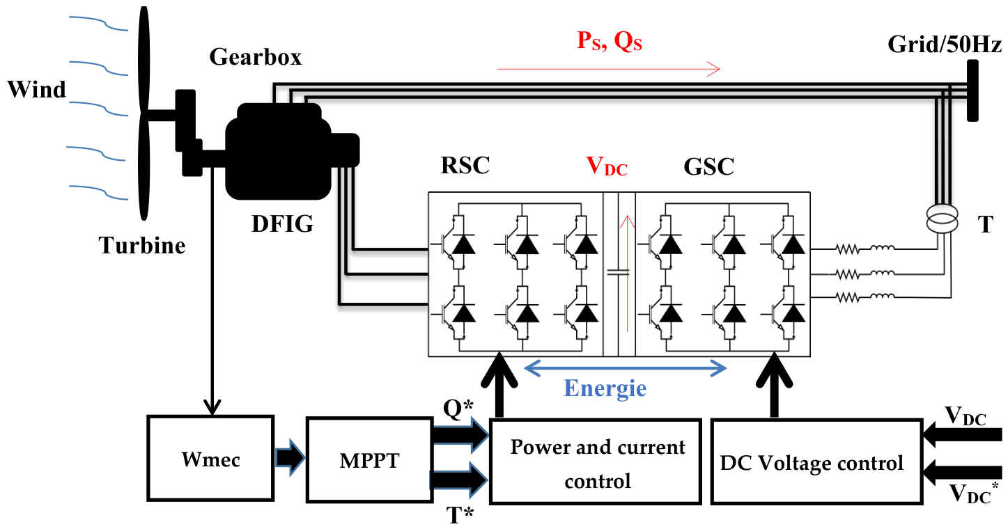
The fundamental structure of WCES depends on the DFIG since it has a clear structure, flexible power regulation, and a small converter capacity, so these generators are frequently used in variable-speed wind systems. In DFIGs, the stator is directly connected to the main grid, while the RSC is connected with converters. The system’s power losses are particularly high since the converter deals with the rated energy immediately; hence, to reduce the rotor’s electricity losses, the converter offers around 30% of the rated energy within the DFIG. Adopting this method can bring about a discounted machine value compared to other technologies, as shown in Figure 1. The RSC guarantees a decoupled stator power regulation (Ps and Qs) [69,70,71]. MPPT method determines the turbine’s speed to generate the most power attainable. It will be a question of controlling energy exchanges and, in particular, the transfers of Ps and Qs sent to the grid in the case of the vector control of the DFIG. The RSC control principle provides for indirect control of power (Ps and Qs) and maximum WE extraction. Traditional PI controllers implement the DFIG’s power control. Rotor currents are thus controlled using PI controllers [72,73]. Figure 2 presents the topology of DFIG-based WECS.
The stator and rotor voltage equations can be expressed using matrix notation as follows [74]:
V s = R s I s + d φ s d t
V r = R r I r + d φ r d t
With:
R s = R s 0 0 0 R s 0 0 0 R s ,   R r = R r 0 0 0 R r 0 0 0 R r
where Rs and Rr denote resistances of stator and rotor windings; Vs and Vr represent stator and rotor voltage, respectively. Is and Ir denote the stator current and rotor current, respectively. Φ s and Φ r represent stator flux and rotor, respectively.
The instantaneous stator and rotor fluxes per phase are given by:
[ φ s ] = [ L s · I s + M s r I r ]
[ φ r ] = [ L r · I r + M r s I s ]
where Ls and Lr are the stator and rotor inductance matrices, respectively, as defined below:
[ L s ] = l s M s M s M s l s M s M s M s l s ,   L r = l r M r M r M r l r M r M r M r l r
The mutual inductance matrix can be expressed as:
[ M s r ] = M c o s ( θ r ) c o s ( θ r + 2 π 3 ) c o s ( θ r + 2 π 3 ) c o s ( θ r + 2 π 3 ) c o s ( θ r ) c o s ( θ r + 2 π 3 ) c o s ( θ r + 2 π 3 ) c o s ( θ r + 2 π 3 ) c o s ( θ r )
where M is maximum value of the mutual inductance between a stator phase and a rotor phase, Ms is the mutual inductance between two distinct stator phases, Mr is the mutual inductance between two distinct rotor phases, and Msr and Mrs represent the mutual inductances between stator and rotor phases, which depend on the rotor angular position θr. The DQ model of the MADA, described in the reference frame rotating at the stator field speed, is expressed as follows:
V s d = R S i s d + d ф s d d t ω s ф s q V s q = R s i s q + d ф s q d t + ω s ф s d V r d = R r i r d + d ф r d d t ω r ф r q V r q = R r i r q + d ф r q d t + ω r ф r d
Such as:
ф s d = L s i s d + M s r i r d ф s q = L s i s q + M s r i r q ф r d = L r i r d + M s r i s d ф r q = L r i r q + M s r i s q
The electromagnetic torque can be expressed as a function of stator fluxes and currents by the following expression:
T e m = p · M s r I s q · I r d I s d · I r q
where Msr represents mutual inductance between the stator and the rotor, and p is the number of pole pairs.
The active and reactive powers are expressed as follows:
P s = V s d i s d + V s q i s q   Q s = V s q i s d V s d i s q
The stator voltage frequency is determined by the power grid, while the rotor current pulsation is given by:
ω r = ω s p Ω
The mechanical equation of the generator is represented by:
T e m = T r + f r · Ω + J · d Ω d t
where:
Tem: Electromagnetic torque of the machine;
Tr: Load (resisting) torque;
fr: Viscous friction coefficient of the DFIG;
Ω: Rotational speed of the DFIG shaft;
J·dΩ/dt: Moment of inertia of the rotating parts, where J is the inertia of the machine.

3.2. DFIG Modeling with Stator/Rotor Fault (SC Between Turns)

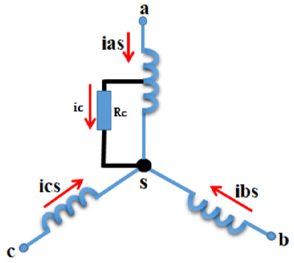
The SC fault is more common in the stator/rotor because it is linked to the SC between the phase turns. It is assumed that several turns (Nt) in phase (a) are short-circuited to model this part. This short-circuited part is represented by the ratio (rcc) from the number of short-circuited turns to the overall number of turns in phase (a), which is entered in the mathematical model guiding the operation of the machine, as can be shown in Figure 3, which shows the three short-circuited stator windings. As a result, the self-inductance and resistance of the faulted phase change, as well as the mutual inductance of that phase, with all the other machine windings. An SC fault in the winding of the stator or the rotor results in a large current in the short turns.
This SC can affect currents in other phases and produce a phase-to-ground and phase-to-phase SC, damaging the equipment. Modeling the DFIG with the fault involves introducing a resistor (Rc) in parallel with the short-circuited turns in the affected phase, as shown in Figure 3 [75,76]. As a result of all this, the resistance matrix of the stator and rotor windings can be rewritten as follows:
R S = ( 1 r C C ) R s 0 0 r C C R S 0 R s 0 0 0 0 R s 0 0 0 0 r C C R S
R r = ( 1 r C C ) R r 0 0 r C C R r 0 R r 0 0 0 0 R r 0 0 0 0 r C C R r
And the mutual inductance matrix becomes the following form:
M s r = M s 1 r c c c o s θ r 1 r c c c o s ( θ r + 2 π 3 ) 1 r c c c o s ( θ r 2 π 3 ) c o s ( θ r 2 π 3 ) c o s θ r c o s ( θ r + 2 π 3 ) c o s ( θ r + 2 π 3 ) c o s ( θ r 2 π 3 ) c o s θ r r c c c o s θ r r c c c o s ( θ r + 2 π 3 ) r c c c o s ( θ r 2 π 3 )
M r s = M r 1 r c c c o s θ r 1 r c c c o s ( θ r 2 π 3 ) 1 r c c c o s ( θ r + 2 π 3 ) c o s ( θ r + 2 π 3 ) c o s θ r c o s ( θ r 2 π 3 ) c o s ( θ r 2 π 3 ) c o s ( θ r + 2 π 3 ) c o s θ r r c c c o s θ r r c c c o s ( θ r 2 π 3 ) r c c c o s ( θ r + 2 π 3 )
where Ms: The magnetizing inductance of the stator winding.
Mr: The magnetizing inductance of the rotor winding.
The proportion of short-circuited turns in stator phase ‘a’ is represented by the coefficient rcc. Consequently, the healthy part corresponds to a fraction (1 − rcc) of the turns. It is also assumed that phases b and c remain intact. Under these conditions, the new stator inductance matrix can be written as follows:
L s s = L f s d i a g 1 r c c 1 1   r c c   + M s 1 r c c 2 1 r c c 2 1 r c c 2 r c c ( 1 r c c ) 1 r c c 2 1 1 2 r c c 2 1 r c c 2 r c c ( 1 r c c ) 1 2 r c c 2 1 r c c 2 r c c 2 r c c 2
If rcc denotes the fraction of short-circuited turns in rotor phase a, then the new rotor inductance matrix can be defined as follows:
L r r = L f r d i a g 1 r c c 1   1   r c c   + M r 1 r c c 2 1 r c c 2 1 r c c 2 r c c ( 1 r c c ) 1 r c c 2 1 1 2 r c c 2 1 r c c 2 r c c ( 1 r c c ) 1 2 r c c 2 1 r c c 2 r c c 2 r c c 2

4. Fault Diagnostic Method and Simulation Results

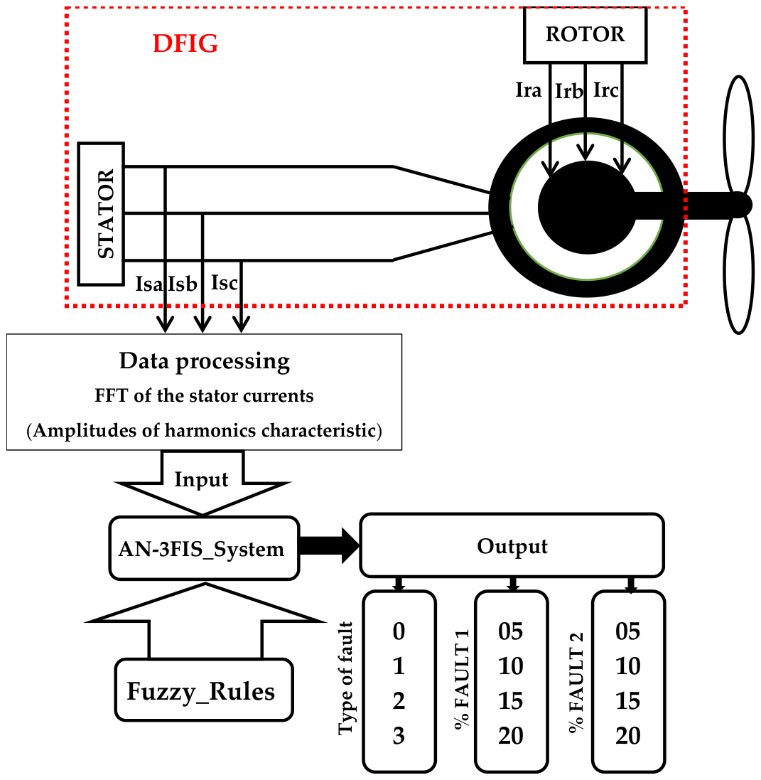
The procedure for detecting and diagnosing rotor and stator short circuits in the WCES DFIG relies on analyzing the machine’s stator current using the AN-3FIS-FFT technique, as shown in Figure 4.
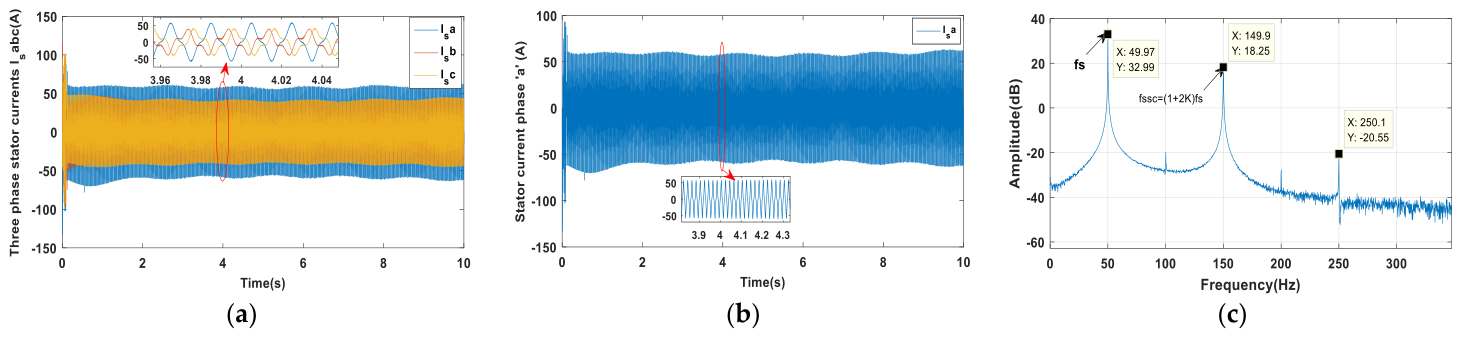
Like other fault detection methods, spectral analysis is one of the simpler methods. In this context, a spectral analysis of the stator current was performed to detect faults occurring in the DFIG [77,78]. The resulting spectral values revealed the effects predicted by theoretical analysis (the occurrence of fault-characteristic harmonics, enabling the fault’s occurrence detection). The SC fault characteristics between the stator (FAULT1) and rotor turns (FAULT2) of the DFIG in WCES for healthy and faulty operation are defined as follows: In the case of healthy DFIG operation, a single harmonic occurs in the current spectrum at a frequency of 50 Hz, which is the fundamental (fs). The imbalance caused by the DFIG stator coil SC fault influences the impedances between the three phases. The stator current spectrum contains, in addition to the fundamental, harmonics characteristic of the stator fault, at whose expression is given by:
f s s c = ( 1 + 2 k ) f s ,       k = 1 , 2 , 4
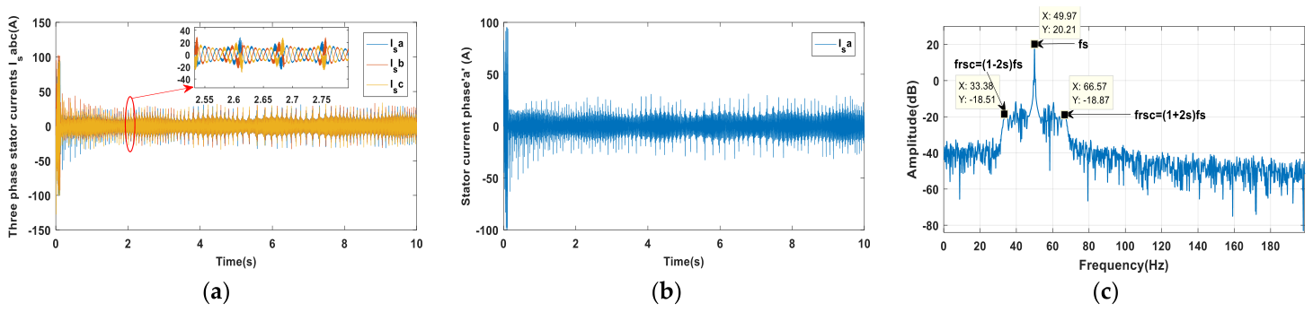
As for the SC fault between rotor turns, for the short-circuit fault between rotor turns, the spectrum of the stator current contains, in addition to the fundamental, new harmonics that appear on both sides of the fundamental. The following expression gives their frequencies:
f r s c = 1 ± 2 k s f s ,       k = 1 , 2 , 4
where:
s is the slip of the machine. The slip s quantifies the difference in rotational speed between the rotor and the stator:
s = f r f s = w s w m w s
where wm is mechanical angular speed, ws is stator angular speed, fr is rotor frequency, and fs is stator frequency.
With:
w m = p Ω
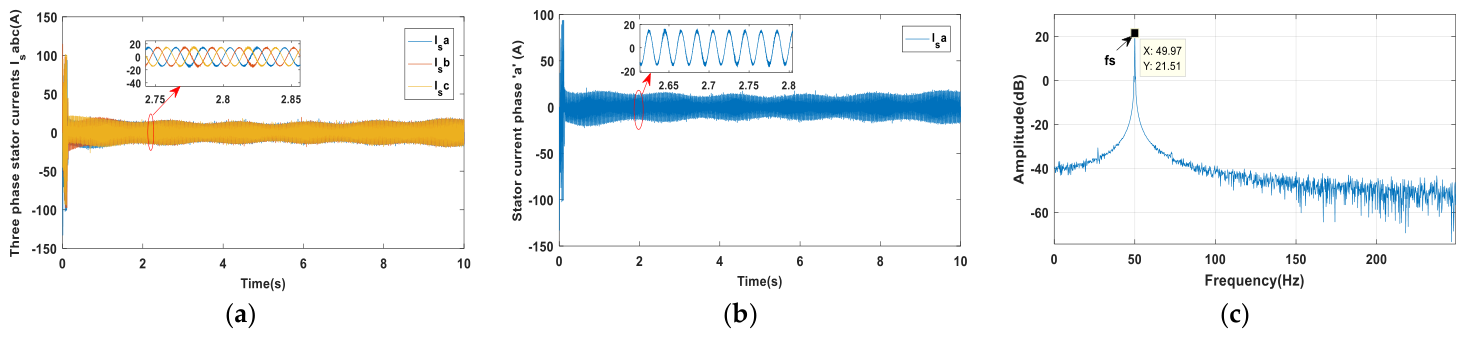
The analysis of stator current response in a DFIG-based WE conversion system for normal and faulty operations are shown in Figure 5, Figure 6 and Figure 7. Time-domain stator currents are considered in the work, along with instantaneous frequency-domain analysis of stator current using FFT for phase a. The magnitude 10% fault severity is selected considering both the cases of rotor short circuit and stator short-circuit fault conditions.
The FFT algorithm is used to simulate DFIG in its three previously mentioned states and clarify each case by spectral analysis, which is applied to a rectangular window of the steady state signal, as shown in subfigures (Figure 5c, Figure 6c and Figure 7c).
Under healthy operating conditions, the DFIG’s three-phase stator currents exhibit symmetrical amplitudes and a constant phase displacement of 120°, confirming the generator’s electrical and magnetic symmetry. After a brief transient period, the time-domain waveforms exhibit a nearly perfect sinusoidal shape with stable amplitude, indicating typical steady-state operation. The fundamental component at the grid frequency (50 Hz) (Figure 5c) dominates the FFT spectrum of stator current phase a, with other harmonic components being insignificant. In addition to acting as a reference signature for fault detection and comparison with faulty operating conditions, this clean spectral profile indicates the lack of electromagnetic disturbances.
Operation under stator short-circuit (S_SC): For a stator ITSC fault with a severity of 10%, the stator current waveforms become clearly unbalanced and distorted. In the time domain, the affected phase exhibits increased amplitude and noticeable waveform deformation. This behavior results from the asymmetry introduced in the stator winding impedance and the consequent disturbance of the air-gap magnetic field.
In the frequency domain, characteristic harmonic components emerge in addition to the fundamental frequency, particularly at odd multiples defined by fssc = (1 + 2k)fs. The appearance and amplification of these harmonics—such as those observed at 150 Hz and 250 Hz (Figure 6c)—constitute a distinct spectral signature of stator winding degradation. These findings confirm the high sensitivity of stator current analysis for detecting stator inter-turn faults.
Operation under rotor short-circuit (R_SC): For a rotor ITSC fault with a severity of 10%, the stator currents are significantly affected despite the fault originating in the rotor circuit. In the time domain, the signals exhibit pronounced high-frequency oscillations and increased ripple, reflecting the strong electromagnetic coupling between the rotor and stator.
In contrast to the stator fault case, the frequency spectrum reveals sideband harmonics distributed symmetrically around the fundamental component, defined by frsc = (1 ± 2ks)fs (Figure 7c). This broader spectral dispersion, along with the presence of symmetric sidebands—such as those appearing at 27.47 Hz and 72.48 Hz—forms a distinctive signature of rotor inter-turn short-circuit faults. These features enable reliable discrimination between stator and rotor faults.
Overall, the clear differentiation of spectral signatures between S_SC and R_SC conditions enhances diagnostic accuracy, supporting more effective condition monitoring and contributing to improved reliability and PQ in WE conversion systems.

4.1. ANFIS Diagnostic Method

This section examines the performance of the proposed diagnosis method for DFIG-based WT. The performance of the method of detecting faults suggested in this paper has been tested by simulation in various possible cases, whether in the healthy mode of the generator or when a short-circuit failure occurs in the stator windings, the rotor windings, or in both of them at the same time, where this simulation is implemented by MATLAB for a DFIG using an ANFIS method. The WCES parameters are shown in Table 2.

4.2. Structure and Designing of the Neuro-Fuzzy Networks System

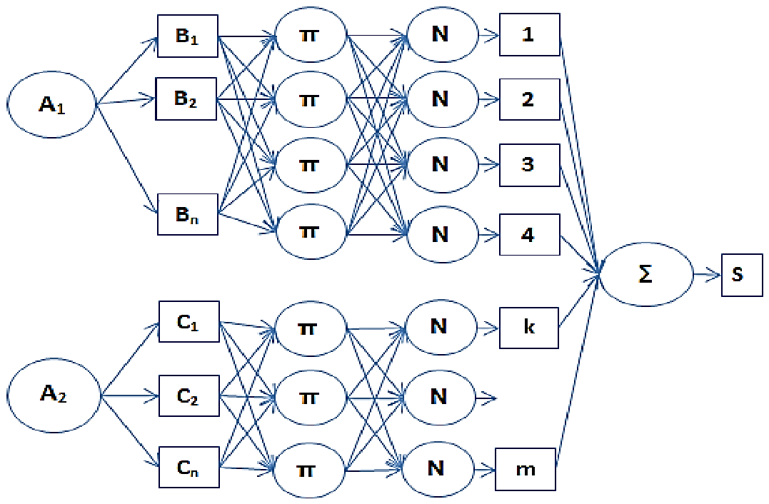
The neuro-fuzzy network used in our work is of the ANFIS type. Figure 8 shows its classical architecture.
The proposed fault diagnosis system is designed around the ANFIS architecture due to its ability to model nonlinear relationships while preserving interpretability through fuzzy rules. In the context of DFIG-based WECS, fault behavior is highly nonlinear and influenced by electromagnetic coupling between stator and rotor circuits, making conventional linear diagnostic methods insufficient.
To address this challenge, three independent ANFIS models are constructed, all sharing the same five frequency-domain inputs but producing distinct outputs. The first ANFIS model is responsible for identifying the fault type, distinguishing between healthy operation, stator ITSC, rotor ITSC, and combined-fault conditions. The second and third ANFIS models estimate the severity percentage of stator and rotor ITSC faults, respectively. This modular configuration avoids output interference, enhances numerical stability, and enables precise tuning of each diagnostic task.
Each ANFIS is initialized using a first-order Sugeno fuzzy inference system. Generalized bell-shaped membership functions are employed to ensure smooth transitions between operating states and to effectively represent the gradual evolution of ITSC faults. The initial fuzzy rule base is generated using grid partitioning, ensuring comprehensive coverage of the input space and the ability to capture subtle fault-induced variations.
The ANFIS receives the following extracted features as input variables:
  • In_amp_h_F: The amplitudes of harmonics characteristic in the healthy state of DFIG (Amp(fs)).
  • In_amp_h_c_S_SC: The amplitudes of harmonics characteristic in the S_SC faults of DFIG (Amp(1 + 2k)fs) with k = 1.
  • In_amp_h_c_S_SC: The amplitudes of harmonics characteristic in the S_SC faults of DFIG (Amp(1 + 2k)fs) with k = 2.
  • In_amp_h_c_R_SC: The amplitudes of harmonics characteristic in the R_SC faults of DFIG (Amp((1 + 2ks)fs))with k = 1.
  • In_amp_h_c_R_SC: The amplitudes of harmonics characteristic in the R_SC faults of DFIG (Amp((1 − 2ks)fs)) with k = 1.
In this study, the input features of the ANFIS were extracted under both healthy operating conditions and the investigated faulty conditions. For each fault type, several severity levels were considered to accurately represent the system behavior under realistic operating scenarios. These severity levels were quantified using the amplitudes of the characteristic harmonic components, denoted as Amp5%, Amp10%, Amp15%, and Amp20%, which correspond to fault severities of 5%, 10%, 15%, and 20%, respectively. This comprehensive dataset was employed to train the ANFIS model.
Three ANFIS models were developed, all using the same five inputs but with different outputs for specific diagnostic tasks. The first model identifies and classifies faults, while the second and third estimate the severity of the first and second detected faults, respectively. The outputs of the three models are defined as follows:
Out ANFIS_network_1 = [
0
1
2
3];
With:
  • 0: health of DFIG.
  • 1: S_SC faults of DFIG.
  • 2: R_SC faults of DFIG.
  • 3: M_SC faults of DFIG.
Out ANFIS_network_2 = [
5
10
15
20];
With:
  • 05: A 05% severity of an S_SC
    fault in the statorof DFIG.
  • 10: A 10% severity of an S_SC
    fault in the statorof DFIG.
  • 15: A 15% severity of an S_SC
    fault in the statorof DFIG.
  • 20: A 20% severity of an S_SC
    fault in the stator of DFIG.
Out ANFIS_network_3 = [
5
10
15
20];
With:
  • 05: A 05% severity of an R_SC fault in the rotorof DFIG.
  • 10: A 10% severity of an R_SC fault in the rotorof DFIG.
  • 15: A 15% severity of an R_SC fault in the rotorof DFIG.
  • 20: A 20% severity of an R_SC fault in the rotor of DFIG.
S_SC: stator short circuit, R_SC: rotor short circuit, and M_SC: combined faults.

4.2.1. Model Structure, Training Settings, Training and Testing Results

A. 
Model_1: Fault-Type Classification
The first-order Sugeno-type ANFIS employs a compact fuzzy rule base consisting of five fuzzy rules, generated to represent the nonlinear relationships between the five input features and the corresponding fault classes. The model uses Gaussian membership functions in the antecedent part and a linear consequent structure, providing sufficient local flexibility while maintaining a relatively compact model architecture. The ANFIS training process combines the least-squares estimation method for identifying the consequent parameters with gradient-descent optimization for adjusting the antecedent parameters. The model was trained for 100 epochs, with checking data evaluated during training to monitor the generalization behavior and obtain a suitable balance between model expressiveness and robustness. The final architecture comprises 68 nodes, 30 linear parameters, and 50 nonlinear parameters, resulting in a total of 80 adjustable parameters.
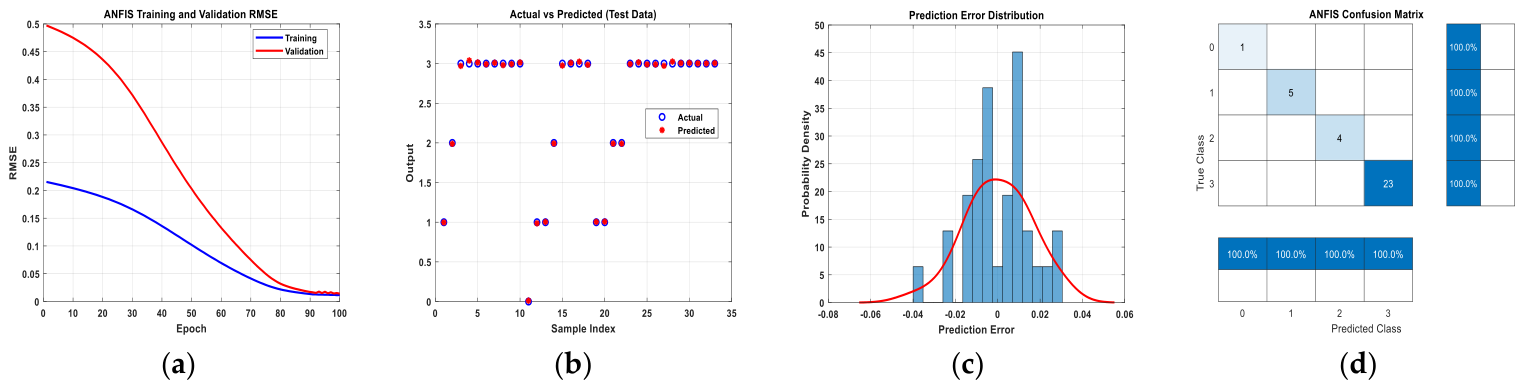
The evolution of the training and checking RMSE over the 100 training epochs is presented in Figure 9a. Both curves exhibit a progressive reduction in error throughout the training process, with the training RMSE decreasing from approximately 0.22 at the beginning of training to a minimum value of 0.011416, while the minimum checking RMSE reaches 0.014018. The close values of the final training and checking errors indicate that the trained model achieves a low prediction error while maintaining a comparable performance on the checking data. Importantly, the curves converge toward very small error values without exhibiting a persistent and substantial divergence between training and checking errors in the final training stages. This behavior suggests that the selected five-rule fuzzy structure provides an adequate representation of the nonlinear input–output relationship while avoiding unnecessary model complexity. The resulting architecture therefore provides a compact ANFIS representation with sufficient modeling capacity for the considered fault-classification problem.
Figure 9b shows the comparison between the predicted and actual outputs for the independent test dataset. The predicted outputs are closely aligned with the corresponding actual class labels across all test samples. The final testing RMSE is 0.015228, which remains very small relative to the numerical separation between the fault classes. In addition, the predicted values show no systematic displacement toward a specific class, indicating consistent classification behavior over the complete test set. The close correspondence between the actual and predicted outputs demonstrates that the trained ANFIS successfully captures the nonlinear decision boundaries associated with the considered fault classes.
The prediction-error distribution is illustrated in Figure 9c. The histogram shows that the prediction errors are concentrated around zero, with most errors distributed within a relatively narrow interval. The limited spread of the residuals and their concentration close to zero indicate a low overall prediction deviation and support the high predictive accuracy observed on the test dataset. The error distribution also does not reveal an evident systematic bias toward either positive or negative prediction errors, suggesting that the model does not consistently overestimate or underestimate the target class values.
Finally, Figure 9d shows the ANFIS confusion matrix derived using the test dataset. It is seen that the ANFIS model perfectly classifies all the samples belonging to the four classes, leading to 1/1 perfect classification in case 0, 5/5 for case 1, 4/4 for case 2, and 23/23 for case 3. Therefore, there are 33 test samples in the diagonal of the confusion matrix and no classification error in the off-diagonal part. Thus, the accuracy rate of the test dataset is 100%. The perfect diagonal structure of the confusion matrix confirms the strong discriminative performance of the trained ANFIS for the tested observations. However, because the dataset is relatively limited and the model contains a substantial number of adjustable parameters relative to the available training observations, the obtained performance should be further examined under controlled perturbations of the input variables. Therefore, a subsequent sensitivity and robustness analysis is performed using the fixed trained ANFIS model, without retraining, to evaluate the stability of its classification performance under variations in the input features.
A.1. 
Sensitivity Analysis of Model_1:
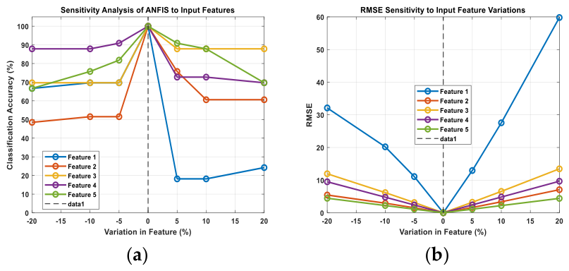
To further assess the stability of the developed ANFIS classifier, a one-at-a-time sensitivity analysis was performed by perturbing each input feature independently by −20%, −10%, −5%, +5%, +10%, and +20%, while keeping the remaining features unchanged and without retraining the ANFIS model. The performance of the unperturbed model at 0% variation was considered the baseline, corresponding to a classification accuracy of 100% and a testing RMSE of 0.015228. As shown in Figure 10a, the response of the classifier varies significantly among the five input features, indicating that their contributions to the learned decision boundaries are not equivalent.
Feature 1 exhibits the highest sensitivity, with the classification accuracy decreasing from 100% at the baseline to 69.70% at −5% and falling sharply to 18.18% at +5% and +10%, while it reaches only 24.24% at +20%. This pronounced degradation is accompanied by the largest increase in RMSE, as shown in Figure 10b, reaching 59.804 at +20% and 32.123 at −20%. Feature 2 represents the second-most influential input, with the accuracy decreasing to 48.48% at −20% and the RMSE increasing to 5.448. In comparison, Features 3 and 4 exhibit relatively greater stability. Feature 3 maintains an accuracy of 87.88% for positive variations up to +20%, whereas Feature 4 maintains 87.88–90.91% accuracy for negative variations but decreases to 69.70% at +20%. Feature 5 shows an intermediate sensitivity, retaining 81.82% and 90.91% accuracy at −5% and +5%, respectively, although its performance decreases to approximately 67–70% at ±20%. Based on the maximum degradation from the baseline, the sensitivity ranking is Feature 1 > Feature 2 > Feature 5 > Features 3 ≈ Feature 4.
The corresponding RMSE trends in Figure 10b support the accuracy-based observations, since larger perturbations generally produce larger prediction errors, particularly for Feature 1. These results demonstrate that the classifier relies more strongly on Features 1 and 2 for maintaining its learned class separation, whereas Features 3 and 4 have a comparatively lower influence on classification stability. However, the results also show that the model does not maintain its baseline performance under large perturbations, and therefore the obtained 100% baseline accuracy should not be interpreted as unconditional robustness. Moreover, several ±20% perturbations extend beyond the input ranges represented in the original training data, as indicated by the evalfis-range warnings. Accordingly, the substantial degradation observed at these levels should be interpreted as the combined effect of input sensitivity and extrapolation beyond the learned feature domain. Overall, the sensitivity analysis provides a quantitative assessment of the dependence of the ANFIS decision process on its input features and identifies Feature 1 as the dominant sensitivity factor, while Features 3 and 4 exhibit comparatively greater stability under the investigated perturbations.
A.2. 
Robustness Analysis under Measurement Noise
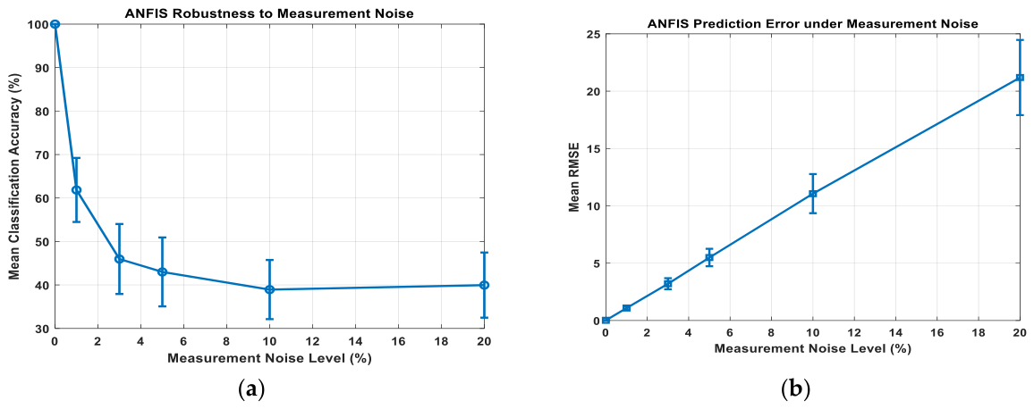
To further assess the reliability of the proposed diagnostic framework under non-ideal measurement conditions, a Monte Carlo robustness analysis was performed by introducing random perturbations into the five FFT-based input features. Unlike the sensitivity analysis, which evaluates the individual influence of each spectral feature, this analysis investigates the overall response of the trained ANFIS model to simultaneous input disturbances. For each perturbation level (1%, 3%, 5%, 10%, and 20%), 100 independent Monte Carlo trials were conducted, while the trained ANFIS model was kept fixed without retraining or parameter adjustment. The mean and standard deviation of the classification accuracy and RMSE were calculated to quantify the diagnostic stability under increasing measurement uncertainty. Table 3 presents the robustness performance of the ANFIS diagnostic model under random input disturbances.
The robustness results are summarized in Table 3 and illustrated in Figure 11a,b. Under nominal conditions, the ANFIS model achieved 100% classification accuracy with an RMSE of 0.0152. As the magnitude of the random input perturbation increased, the classification accuracy generally decreased, reaching 61.85%, 45.97%, 43.00%, and 38.94% at perturbation levels of 1%, 3%, 5%, and 10%, respectively. At 20% perturbation, the mean accuracy was 39.97%. In contrast, the mean RMSE exhibited a clear increasing trend, rising from 0.0152 under nominal conditions to 1.0885, 3.2047, 5.4910, 11.0621, and 21.1877 at 1%, 3%, 5%, 10%, and 20% perturbation, respectively. These results demonstrate that increasing measurement disturbances progressively affect both the diagnostic decision and the numerical accuracy of the ANFIS output.
The observed degradation can primarily be attributed to the increasing deviation of the perturbed feature vectors from the data distribution encountered during model development. At higher perturbation levels, some input features may extend beyond the ranges represented in the training data, forcing the ANFIS model to operate, at least partially, outside its learned input domain. Accordingly, the robustness analysis provides a quantitative characterization of the model’s tolerance and degradation behavior under measurement uncertainty, rather than implying unrestricted robustness to severe disturbances. Importantly, no retraining or parameter adjustment was performed during these experiments. Therefore, the reported degradation directly reflects the response of the trained diagnostic model to increasing levels of input perturbation.
It should also be emphasized that the proposed framework was developed using data generated under variable wind-speed conditions. Consequently, variations in wind speed are inherently represented in the training and evaluation datasets, providing the model with a degree of robustness to this operating-condition variability. The measurement-noise analysis complements this inherent robustness by explicitly quantifying the sensitivity of the diagnostic performance to perturbations in the measured input variables, while keeping the trained ANFIS model unchanged. This distinction is important because robustness to operating-condition variations and robustness to measurement uncertainty represent different aspects of diagnostic reliability. The present study focuses on these two aspects within the considered experimental framework. A more comprehensive assessment involving specific grid disturbances, load variations, sensor-specific uncertainty models, and uncertainties in model parameters would require additional scenarios and dedicated experimental analyses. These aspects are therefore left for future investigations.
A.3. 
Comparative evaluation with conventional machine-learning methods
To further assess the effectiveness of the proposed fault-type classification approach, a quantitative comparison was performed with two representative machine-learning classifiers, namely Support Vector Machine (SVM) and Random Forest (RF). For a fair comparison, all three classifiers were evaluated using the same five FFT-based spectral features, the same four fault classes, and identical training and testing partitions. The evaluation considered Accuracy, Macro-Precision, Macro-Recall, Macro-F1 score, Balanced Accuracy, and RMSE. In addition, the training and per-sample inference times were measured to assess the computational suitability of the investigated approaches for online fault diagnosis.
As reported in Table 4, the proposed ANFIS achieved a classification accuracy of 100%, with a Macro-F1 score and Balanced Accuracy of 1.0000. This performance is equivalent to that of RF and higher than that obtained by SVM, which achieved 90.91% accuracy, a Macro-F1 score of 0.8776, and a Balanced Accuracy of 0.8500. The proposed ANFIS also produced a very low RMSE of 0.0152, indicating a highly consistent correspondence between its numerical output and the target fault classes. These results demonstrate that the proposed fuzzy inference-based classifier can effectively discriminate among the considered healthy, stator-fault, rotor-fault, and combined-fault conditions.
From the computational perspective, RF required the shortest training time (1.97 s), followed by SVM (2.65 s) and ANFIS (4.30 s). However, training is performed offline and therefore has less significance for online diagnostic operation. In contrast, inference time is directly relevant to real-time monitoring. The proposed ANFIS required only 3.88 ms per sample, compared with 8.49 ms/sample for RF and 9.94 ms/sample for SVM. Thus, although ANFIS required a slightly longer offline training time, it provided substantially faster online inference than both benchmark classifiers while maintaining the highest classification performance observed in the comparison. Overall, the comparative results indicate that the proposed ANFIS provides a favorable balance between diagnostic ac-curacy and online computational efficiency. In particular, it achieved the same classifi-cation performance as RF while reducing the inference time by approximately 54.3%, and it outperformed SVM in both classification performance and inference speed. These findings support the suitability of the proposed ANFIS classifier for rapid fault-type identification under the considered simulation conditions. Overall, the comparative results indicate that the proposed ANFIS provides a favorable balance between diag-nostic accuracy and online computational efficiency. In particular, it achieved the same classification performance as RF while reducing the inference time by approximately 54.3%, and it outperformed SVM in both classification performance and inference speed. These findings support the suitability of the proposed ANFIS classifier for rapid fault-type identification under the considered simulation conditions.
From the computational perspective, RF required the shortest training time (1.97 s), followed by SVM (2.65 s) and ANFIS (4.30 s). However, training is performed offline and therefore has less significance for online diagnostic operation. In contrast, inference time is directly relevant to real-time monitoring. The proposed ANFIS required only 3.88 ms per sample, compared with 8.49 ms/sample for RF and 9.94 ms/sample for SVM. Thus, although ANFIS required a slightly longer offline training time, it provided substantially faster online inference than both benchmark classifiers while maintaining the highest classification performance observed in the comparison.
Overall, the comparative results indicate that the proposed ANFIS provides a favorable balance between diagnostic accuracy and online computational efficiency. In particular, it achieved the same classification performance as RF while reducing the inference time by approximately 54.3%, and it outperformed SVM in both classification performance and inference speed. These findings support the suitability of the proposed ANFIS classifier for rapid fault-type identification under the considered simulation conditions.
B. 
Model _2: Stator-Fault Severity Regression
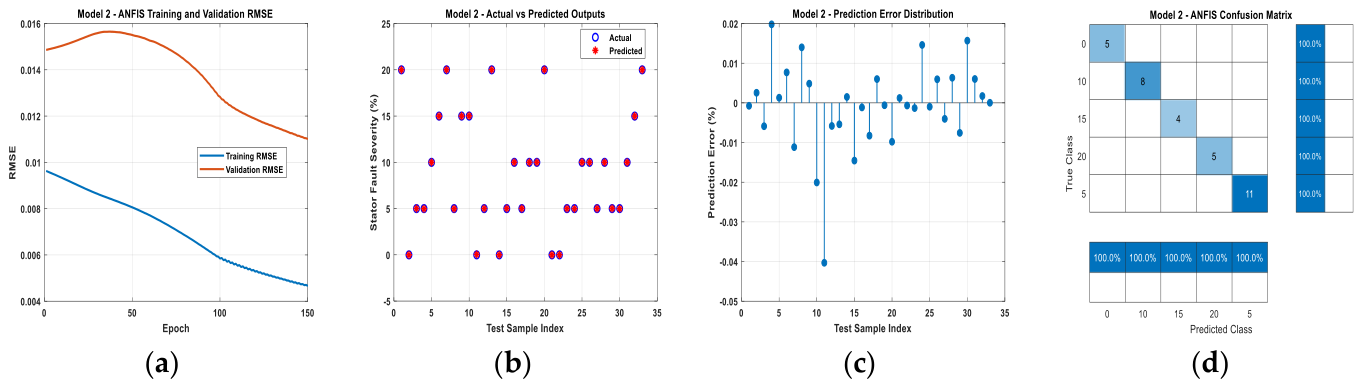
Figure 12, together with the numerical performance indicators, provides a comprehensive evaluation of the ANFIS model in terms of accuracy, convergence behavior, and generalization capability. In terms of quantitative performance, the training RMSE is 0.00466%, while the checking RMSE is 0.01101%. Both values are very low, indicating small prediction errors and a limited generalization gap. The resulting checking error remains sufficiently small relative to the considered stator-fault severity levels, confirming the model’s ability to accurately estimate the fault severity.
The absolute difference is only 0.00635 percentage points, despite the checking RMSE being almost 2.36 times higher than the training RMSE. This suggests that despite the small amount of accessible examples, the model has high generalization power. The findings imply that, without showing significant overfitting, the suggested neuro-fuzzy model effectively represents the nonlinear relationship between the retrieved spectral features and stator-fault severity.
From a structural perspective, the final ANFIS model consists of 116 nodes and 144 adjustable parameters, including 54 linear parameters and 90 nonlinear parameters, governed by 9 fuzzy rules. The model was trained using 77 samples and evaluated using 33 checking samples. Although the number of training samples is smaller than the total number of adjustable parameters, as indicated by the training warning, the obtained convergence behavior and low checking error demonstrate that the hybrid learning algorithm was able to identify the relevant input–output relationships while maintaining stable predictive performance.
As shown in Figure 12a, the training RMSE decreases from approximately 0.00963% at the beginning of training to 0.00466% after 150 epochs. The checking RMSE initially exhibits a slight increase, reaching approximately 0.01565%, before progressively decreasing to its minimum value of 0.01101% toward the end of the training process. The eventual reduction of the checking error, together with the absence of divergence between the two curves, indicates that the training process converges toward a model with good generalization capability. The relatively small difference between the final training and checking errors further supports the numerical stability of the obtained solution.
Figure 12b further supports the numerical results by showing a strong agreement between the actual and predicted outputs for the complete checking dataset. The predicted values closely coincide with the corresponding target severity levels of 0%, 5%, 10%, 15%, and 20%. This close correspondence demonstrates that the learned fuzzy rules provide accurate severity estimation over the complete range of considered stator fault conditions rather than being limited to a specific severity level. The result is consistent with the low checking RMSE of 0.01101% and checking MAE of 0.00750%.
The prediction-error distribution in Figure 12c provides additional evidence of the model’s predictive behavior. Most errors are distributed around zero, indicating limited systematic bias. Although several individual samples exhibit larger positive or negative deviations, these errors remain isolated and have only a negligible effect on the overall prediction performance, as reflected by the very low checking RMSE of 0.01101%. The approximately symmetric distribution of positive and negative deviations also indicates that the model does not exhibit a pronounced systematic tendency to overestimate or underestimate the fault severity.
Finally, the confusion matrix in Figure 12d demonstrates the discriminative capability of the proposed model when the continuous ANFIS outputs are mapped to the five predefined severity classes. All five classes—0%, 5%, 10%, 15%, and 20%—achieve a 100% class-wise recognition rate, with no misclassified samples. Specifically, the diagonal elements contain 5, 11, 8, 4, and 5 correctly classified samples, respectively, resulting in 33 correctly classified samples out of 33, and consequently an overall classification accuracy of 100%. Furthermore, the obtained Macro-Precision, Macro-Recall, and Macro-F1 score are all equal to 1.0000. This result indicates clear separability among the considered stator-fault severity levels. Nevertheless, the confusion matrix is considered complementary to the regression metrics, since perfect discrete-class recognition does not imply zero continuous prediction error, as confirmed by the checking RMSE of 0.01101% and MAE of 0.00750%.
B.1. 
Sensitivity analysis of Model_2:
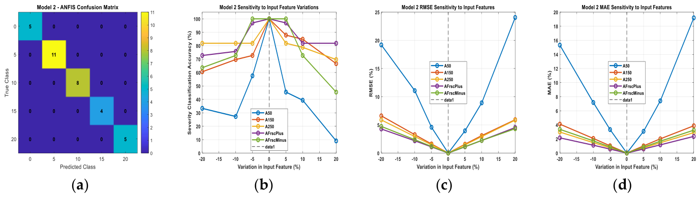
A sensitivity analysis was performed to investigate the robustness of the trained Model_2 to perturbations of the five spectral inputs, A50, A150, A250, AFrsc+ and AFrsc−. Each feature was varied independently by −20%, −10%, −5%, +5%, +10% and +20% while the trained ANFIS parameters were fixed and not retrained. Under the nominal condition (0% variation), the model was able to maintain its baseline performance with RMSE = 0.011008, MAE = 0.007503 and classification accuracy = 100%.
The results show a clear difference in sensitivity among the input features. A50 was the most sensitive feature with accuracy falling to 9.09% with +20% perturbation and an overall maximum degradation of 90.91 percentage points. The RMSE and MAE reached maximum values of 24.0566 and 19.1961, respectively. AFrsc− achieved the second-highest sensitivity with a drop of 54.55 percentage points in accuracy. The corresponding degradations for A150 and A250 were 39.39 and 30.30 percentage points, respectively.
In contrast, AFrsc+ exhibited the highest robustness according to the adopted perturbation criterion. Its maximum accuracy degradation was only 27.27 percentage points, while its maximum RMSE and MAE were 4.5347 and 2.3721, respectively. Therefore, the sensitivity ranking based on accuracy degradation is: A50 > AFrsc− > A150 > A250 > AFrsc+.
Overall, the sensitivity analysis confirms that the model is most dependent on A50, whereas AFrsc+ provides the greatest tolerance to input perturbations. The asymmetric response observed for positive and negative variations also reflects the nonlinear mapping established by the ANFIS model.
Figure 13 presents the sensitivity and robustness characteristics of Model_2 under independent perturbations of the five spectral input features. Figure 13a shows the baseline confusion matrix, where all 33 testing samples are correctly assigned to the five severity levels (0%, 5%, 10%, 15%, and 20%), yielding an accuracy of 100% under the nominal condition. Figure 13b illustrates the corresponding variation in classification accuracy as each input feature is independently perturbed from −20% to +20%. The A50 curve exhibits the strongest degradation, with accuracy decreasing from 100% under the nominal condition to 9.09% at +20%, whereas AFrsc+ shows the most stable response, retaining 96.97% accuracy at both −5% and +5% perturbations. Figure 13c and Figure 13d show the associated RMSE and MAE responses, respectively, and confirm the same sensitivity trend. In particular, perturbing A50 produces the largest prediction errors, with RMSE and MAE reaching 24.0566 and 19.1961, respectively, while AFrsc+ results in the lowest maximum RMSE and MAE of 4.5347 and 2.3721. Overall, the figure demonstrates that the trained ANFIS model exhibits non-uniform sensitivity to the spectral inputs, with A50 being the most sensitive feature and AFrsc+ the most robust according to the adopted accuracy-degradation criterion.
B.2. 
Robustness analysis under measurement noise
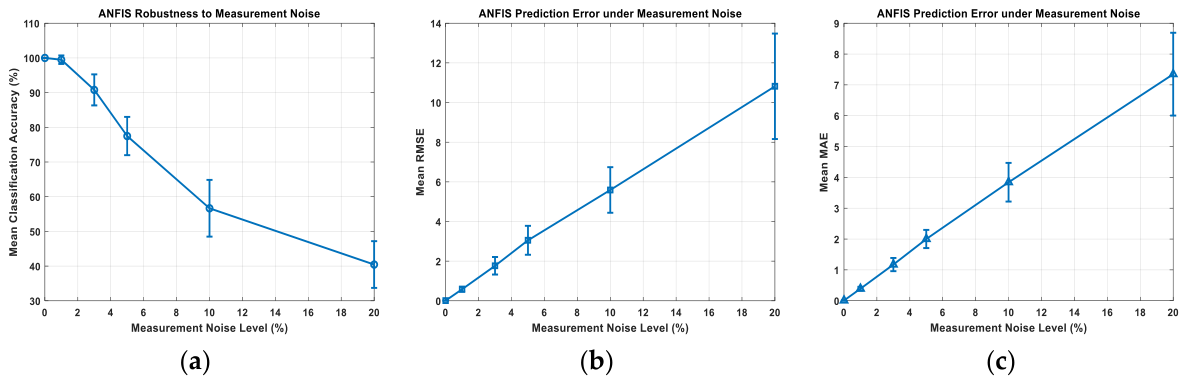
To assess the robustness of Model_2, the five extracted spectral features were perturbed with Gaussian noise and the trained ANFIS model was kept fixed without retraining. A Monte Carlo procedure with 100 independent trials was performed at 0%, 1%, 3%, 5%, 10% and 20% levels of perturbation. The quantitative results are shown in Table 5. The model has 100% classification accuracy under the nominal condition (0% perturbation) with RMSE 0.01101 and MAE 0.00750. At 1% perturbation, the accuracy is almost unchanged at 99.48%, which corresponds to only 0.52 percentage points of degradation. With 3% perturbation, the model still achieves 90.79% accuracy, which shows that it is robust to moderate measurement uncertainties. With further increase in the perturbation, the performance degrades gradually to 77.48%, 56.67% and 40.45% accuracy at 5%, 10% and 20%, respectively. Meanwhile, under nominal conditions, the mean RMSE and MAE are increased from 0.01101 and 0.00750 to 10.81901 and 7.34748 at 20% perturbation. These results confirm that Model_2 has good robustness against low-level measurement uncertainty while severe input perturbations have a significant impact on both severity estimation and severity-class recognition.
The robustness trends are further illustrated in Figure 14a,c. Figure 14a shows the progressive decrease in mean classification accuracy with increasing measurement noise, while Figure 14b,c show the corresponding increase in mean RMSE and MAE. The error bars represent the standard deviation obtained from the 100 Monte Carlo trials, reflecting the variability of the model response under repeated perturbations. The limited variation at 1% and 3% noise levels, together with the small accuracy degradation reported in Table 4, demonstrates stable model behavior under low-to-moderate measurement uncertainty. In contrast, the pronounced increase in prediction errors and accuracy degradation at 10% and 20% perturbations indicates that severe measurement disturbances exceed the effective robustness range of the trained ANFIS model.
B.3. 
Comparative Evaluation with Conventional Machine-Learning Regression Methods
To assess the effectiveness of the proposed Model_2 for stator-fault severity estimation, it was compared with SVR and RF regression using the same five FFT-based features and identical training/testing datasets. The comparison considered regression accuracy, severity-level accuracy, and computational time. Table 6 presents a quantitative comparison between the proposed ANFIS model and the SVR and Random Forest Regression models for estimating the severity of stator faults.
As illustrated in Table 6, the suggested ANFIS clearly achieved the best regression performance, with a MAE of 0.0075%, RMSE of 0.0110%, R2 of 0.999997, and MAPE of only 0.1028%. SVR provided the second-best performance, whereas RF showed considerably larger prediction errors. After converting the continuous outputs into the predefined severity levels (0%, 5%, 10%, 15%, and 20%), ANFIS achieved 100% severity accuracy and a Macro-F1 of 1.0000, compared with 96.97% and 0.9691 for SVR, and 51.52% and 0.4648 for RF.
Regarding computational cost, SVR required the shortest training time (0.2128 s), followed by RF (0.7062 s) and ANFIS (2.4369 s). However, ANFIS achieved the lowest inference time (0.0417 ms/sample), making it approximately 6.8 times faster than SVR and 41 times faster than RF during online prediction. Therefore, although ANFIS requires longer offline training time, it provides substantially superior estimation accuracy and faster online inference, supporting its suitability for real-time stator-fault severity estimation.
C. 
Model_3: Rotor-Fault Severity Regression
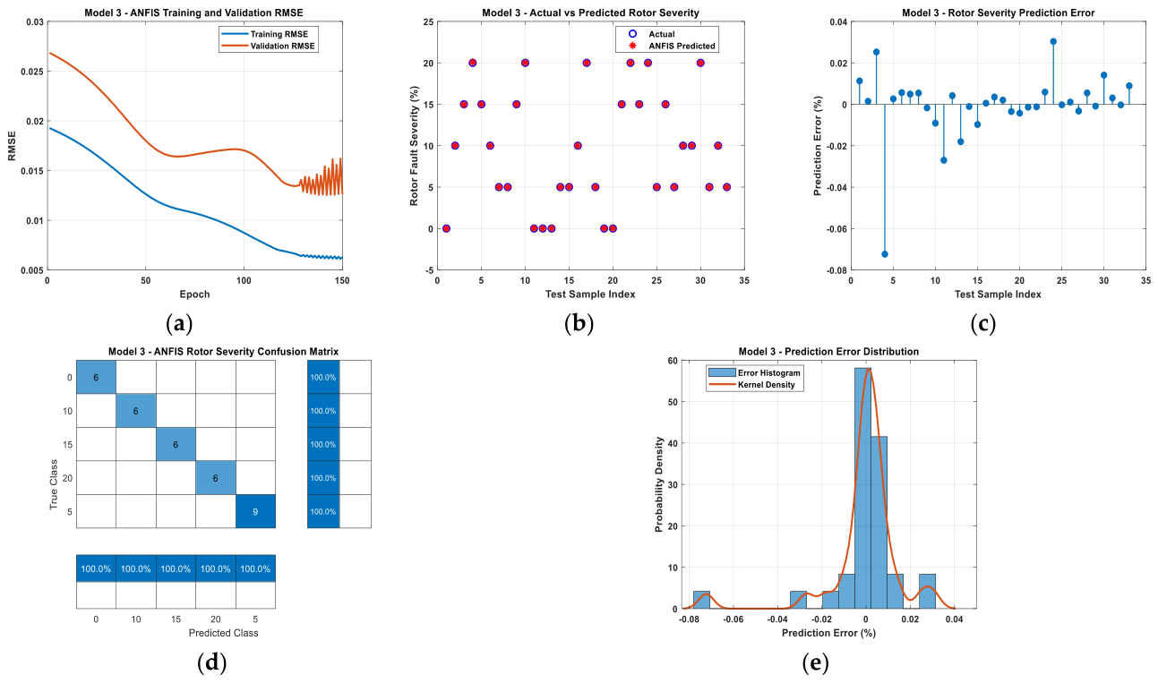
The RMSE curves for the training and checking datasets in Figure 15a show a continuous decrease followed by stable convergence, indicating a well-behaved learning process. The minimum training RMSE reached 0.006111, while the minimum checking RMSE was 0.012505 at epoch 142. The final testing performance yielded an RMSE of 0.016228 and an MAE of 0.008790, confirming the low prediction error and good generalization capability of the proposed ANFIS model.
Figure 15b shows a close agreement between the actual and predicted rotor-fault severity levels for all considered conditions (0%, 5%, 10%, 15%, and 20%). The predictions are almost perfectly aligned with the reference values, resulting in a testing R2 of 0.999994 and a very low MAPE of 0.067586%. These results demonstrate the capability of the proposed ANFIS model to accurately capture the nonlinear relationship between the extracted spectral features and rotor-fault severity.
The prediction error shown in Figure 15c remains tightly distributed around zero, with limited deviations and no evident systematic bias. This behavior is consistent with the low-testing MAE of 0.008790, confirming the numerical stability of the severity estimation. Figure 15e further illustrates this behavior through the prediction-error histogram and kernel-density estimate, where the highest concentration of errors is located close to zero, indicating low overall error dispersion.
According to the confusion matrix in Figure 15d, all test samples were correctly assigned to their corresponding severity levels, yielding 100% severity accuracy. The model also achieved Macro-Precision, Macro-Recall, Macro-F1 score, and Balanced Accuracy of 1.0000. Overall, the combined results in Figure 15a–e, together with the very low regression errors and R2 of 0.999994, demonstrate the strong capability of the proposed ANFIS model for accurate rotor-fault severity estimation under the considered simulation conditions.
C.1. 
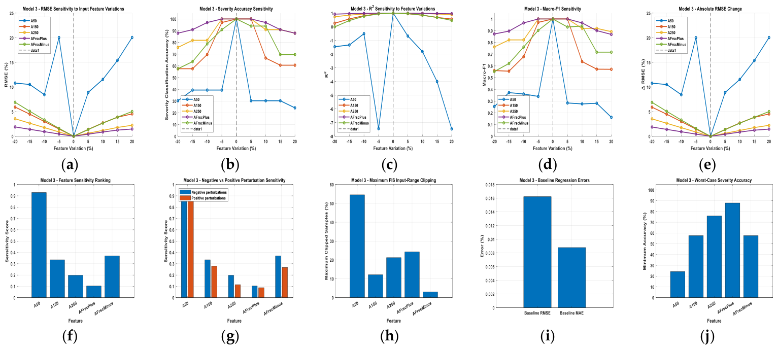
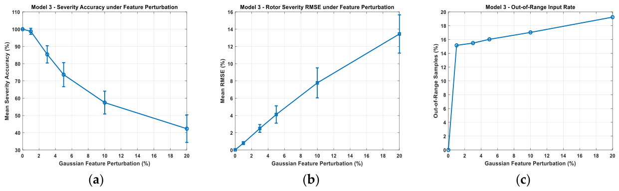
Sensitivity and robustness analysis of Model_3:
Figure 16 presents the sensitivity and robustness analysis of Model_3 rotor-fault severity regression under controlled perturbations of ±20% applied independently to the five spectral features. The baseline model achieved excellent performance, with RMSE = 0.016228%, MAE = 0.008790%, (R2) = 0.999994, 100% severity-level accuracy, and Macro-F1 = 1.0000. As shown in Figure 16a–e, the model exhibited a clearly non-uniform and nonlinear response to feature perturbations. A50 was the most sensitive feature, with an overall sensitivity score of 0.9291, followed by AFrsc− (0.3689), A150 (0.3349), A250 (0.1973), and AFrsc+ (0.1029), as summarized in Figure 16f. Perturbing A50 by −20% and +20% increased RMSE to 10.803% and 20.052%, respectively, while (R2) decreased to −1.456 and −7.461, confirming its dominant influence on the learned severity mapping. In contrast, AFrsc+ showed the highest robustness, maintaining RMSE below 1.91% and (R2 > 0.92) even under ±20% perturbation. A250 also exhibited relatively good robustness, whereas A150 and AFrsc− produced intermediate degradation levels.
The comparison of negative and positive perturbations in Figure 16g confirms a directional and nonlinear sensitivity, particularly for A50. Figure 16h further shows that input-range clipping contributes to performance degradation, with the maximum clipping ratio reaching 54.55% for A50 at +20%; however, clipping alone does not fully explain the observed sensitivity, indicating an additional contribution from the nonlinear ANFIS rule mapping. The baseline error levels in Figure 16i confirm the high nominal accuracy, while the worst-case results in Figure 16j highlight the substantially greater vulnerability of A50 compared with the other features. Overall, the analysis demonstrates that Model_3 maintains good robustness to perturbations in most spectral inputs, while A50 requires the highest measurement reliability because of its dominant influence on rotor-fault severity estimation.
C.2. 
Robustness analysis under measurement noise
To check how robustness Model_3 is when there is uncertainty in the measurements the five input features that were taken out were changed with noise. The ANFIS model that was already trained stayed the same and was not trained again. A Monte Carlo analysis was performed with 100 tests at different levels of noise, which were 0%, 1%, 3%, 5% 10% and 20%. The inputs that had the noise added were put into the trained model directly. There was no limit set on the values that went beyond what the FIS model could handle. The number of times the inputs went out of range was watched carefully. The results on how strong the models are shown in Table 7.
Under nominal conditions, Model_3 achieves 100% classification accuracy with an MAE of 0.008790, an RMSE of 0.016228, and an R2 of 0.999994, confirming the high predictive consistency of the fixed baseline model. At 1% perturbation, the accuracy remains high at 98.76%, with only 1.24 percentage points of degradation and R2 still equal to 0.986016. However, the effect of measurement noise becomes progressively more pronounced beyond this level. At 3% and 5% perturbation, the accuracy decreases to 85.39% and 73.64%, respectively, while RMSE increases to 2.494919 and 4.112547. At 10% perturbation, the accuracy falls to 57.45% and R2 becomes negative (−0.335806), indicating a substantial loss in regression quality. Under the most severe perturbation of 20%, the accuracy decreases to 42.33%, accompanied by RMSE and MAE values of 13.446344 and 9.228069, respectively, while R2 reaches −2.907093. Thus, Model_3 exhibits strong robustness to very low measurement perturbations, whereas perturbations above approximately 3–5% produce a marked deterioration in both severity estimation and severity-class recognition.
The FIS operating range had an effect that was looked into by dividing the samples that were changed into two groups: in range and out of range. When the samples were changed by 1% 15.15% of them were already found to be out of range. This number went up slowly to 19.24% when the samples were changed by 20%. Even though the number of out-of-range samples did not go up much, the predictions got a lot worse. This shows that the FIS range being violated is not the reason the predictions are not as good. The accuracy of the samples that were still in range went down from 98.55% at 1% change to 37.75% at 20% change. This means that noise in the measurements can really affect what the model predicts, even when the changed inputs are still within the FIS operating ranges.
On the one hand, the samples that were out of range still had somewhat high accuracy when the changes were small or moderate. The accuracy went down from 100.00% at 1% change to 94.12% at 5% change. Then, it went down to 81.97% and 61.52% when the changes were 10% and 20%, respectively. This means that reason for the predictions getting worse is mostly because the changes are increasing, not just because the inputs are out of range.
The trends presented in Figure 17 further confirm the progressive deterioration of Model_3 as the perturbation level increases. Figure 17a shows a clear decrease in classification accuracy, from 100% under nominal conditions to 98.76%, 85.39%, 73.64%, 57.45%, and 42.33% at 1%, 3%, 5%, 10%, and 20% perturbation, respectively. Figure 17b exhibits the corresponding increase in RMSE, indicating a progressive deterioration in the continuous severity estimation. The error bars represent the standard deviation across the 100 Monte Carlo trials and show increasing variability at higher perturbation levels, particularly at 10% and 20%. Figure 17c shows that the proportion of out-of-range samples increases from 0% at nominal conditions to 19.24% at 20% perturbation. The relatively gradual increase in out-of-range occurrence, compared with the much stronger degradation in accuracy and regression error, supports the conclusion that the loss of robustness is mainly driven by the magnitude of feature uncertainty rather than by FIS range violations alone.
The overall robustness analysis shows that Model_3 is robust under low-level measurement uncertainty, especially with 1% perturbation. However, the performance of Model_3 degrades significantly under moderate-to-severe perturbations. The results indicate that the level of measurement uncertainty should be kept low to maintain the accuracy of the rotor-fault severity estimation and classification.
C.3. 
Comparative Evaluation with Conventional Machine-Learning Regression Methods
In order to further validate the performance of the proposed Model_3, comparisons were made between the results of the severity estimation of rotor faults with the results from SVR and Random Forest models. Table 8 summarizes the main performance and computational metrics of each model.
The ANFIS method has performed the best amongst the given methods according to Table 8. The calculated RMSE, MAE, and R2 values for ANFIS were found to be 0.016228%, 0.008790%, and 0.999994 with MAPE being only 0.067586%. This means that there was very little deviation between the estimated rotor-fault severity levels and actual levels. In contrast, both SVR and RF have shown sizeable errors with RMSE values of 1.090398% and 3.157485%, respectively. The superiority in the performance of ANFIS was also confirmed at the level of severity classification where it attained a rate of 100% and Macro-F1 of 1.0000, whereas SVR scored 93.94% and 0.9143 and RF scored 84.85% and 0.7357, respectively. It should be noted that benchmark methods were less discriminate at a 20% level of severity, whereas ANFIS managed to classify all samples correctly.
In terms of computation, SVR needed the least amount of time for training (2.106348 s), then the RF came in at 2.817974 s, and finally ANFIS came last at 3.017180 s in terms of training time taken. Also, SVR and RF predicted more rapidly than ANFIS. However, this computational ease came with a cost as there was a significant decrease in accuracy of estimation. To sum up the results, we can see that proposed ANFIS comes with much higher accuracy and severity-discrimination capability compared to slightly higher computational time in the ranking of methods.
D. 
Computational Complexity and Real-Time Feasibility
The assessment of the computational cost for the novel hierarchical FFT-ANFIS technique was carried out using fixed baseline models without any need for retraining them. Results presented in Table 9 show that in both cases, the three models utilize five spectral inputs and need 5–11 fuzzy rules corresponding to 80–176 overall parameters. The total time required for inference is 0.01547 ms/sample–0.02633 ms/sample; the memory consumption has not exceeded 0.18 MB. It can be inferred that the method is characterized by low computational and memory requirements allowing its use in real-time applications. Since a dedicated embedded hardware has not been used, the embedded implementation has not been tested directly.

4.2.2. Validation Test of Resultants

The results presented in Figure 18 represent a representative subset of the full test database. These selected samples highlight the model’s accuracy, robustness, and generalization capability for ANFIS-based fault diagnosis of generators under a range of operating conditions. The samples cover healthy operation as well as instances of single stator and rotor short-circuit faults with varying severity levels, including combinations of both fault types. This selection provides a comprehensive and scientifically rigorous evaluation of the model’s diagnostic performance.
Under healthy operating conditions (Figure 12a), the fault output converges to 2.358 × 10⁻⁵, while the S_SC and R_SC severity indices remain within the 10−5 to 10−4 range. These very low residuals demonstrate strong noise rejection and a minimal false alarm rate. Methodologically, this behavior indicates an absence of overfitting and confirms that the trained ANFIS model maintains stable discriminative performance when exposed to previously unseen normal data.
The classifier correctly identified type ‘1’ for stator short-circuits (S_SCs) faults at severity levels of 5% and 20% (Figure 18b,c) and provided highly accurate quantitative estimates of fault magnitude. The predicted severity values closely match the injected fault levels, while the rotor fault index remains effectively zero. This clear class separability demonstrates that the nonlinear mapping learned during training successfully captured the intrinsic characteristics of stator faults without any cross-interference from other fault types.
Similarly, for R_SC faults at 10% and 15% severity (Figure 18d–e), the system consistently classifies these events as Class 2 while providing precise severity estimates. The stator-related outputs remain in the 10−6 range, demonstrating excellent fault isolation and minimal cross-sensitivity. This highlights the effectiveness of the fuzzy inference rule base in modeling discrete electro-mechanical fault patterns.
The most technically significant validation results were obtained under combined-fault conditions (M_SC) (Figure 18f–h). In these scenarios, the ANFIS model accurately classified and simultaneously estimated the severity of both S_SC and R_SC faults as a Type 3 fault. The close correspondence between the injected and estimated fault levels (e.g., 15–20%, 5–5%, 15–15%) indicates that the proposed architecture can effectively capture the multidimensional nonlinear coupling effects. This capability is particularly noteworthy, as multi-fault diagnosis is a well-known challenge in intelligent condition monitoring due to the overlapping and interacting features present in each fault signature.

4.3. Discussion Section

The combination of FFT-based harmonic feature extraction and ANFIS networks demonstrated strong diagnostic capability. Stator-current signals were analyzed using FFT to extract characteristic harmonic amplitudes, which were then fed into dedicated ANFIS networks trained to recognize specific fault types, as described in Section 4.2. The system successfully identified each fault type across varying severity levels (5%, 10%, 15%, and 20%), confirming the robustness of the model and its ability to capture nonlinear relationships between harmonic features and fault classes.
The results indicate that the ANFIS models are sensitive to variations in harmonic amplitude corresponding to fault progression. As amplitudes increased (e.g., from Amp5% to Amp20%), the system consistently mapped these changes to higher severity levels, demonstrating that the model not only detects faults but also provides reliable fault quantification—a critical aspect for predictive maintenance.
Thanks to the efficiency of FFT for feature extraction and the relatively low computational demands of ANFIS, the hybrid approach effectively handles uncertainty and imprecision in measurement data. The FL membership functions on smooth decision boundaries, allowing realistic modeling of system behavior, particularly in borderline cases or during gradual fault development. The ANFIS-FFT method also proved resilient to variations in operating conditions, including WSs between 7 and 12 m/s.
The system achieved high performance metrics, including rapid response times and classification accuracies reaching 100% for each fault type. The integration of FL with neural networks enabled precise extraction of fault-specific harmonics while effectively managing measurement uncertainty. These capabilities make the system suitable for real-time condition monitoring, though experimental validation under practical operating conditions remains a task for future work.
Therefore, the findings show that the proposed strategy achieves a high degree of diagnostic precision in the investigation, while also bridging the gap between qualitative fault detection and quantitative multi-fault severity evaluation, which many of the present fault diagnosis studies do not address sufficiently from a methodical standpoint.

4.4. Comparative Analysis with Existing Methods

To further assess the effectiveness of the proposed ANFIS-FFT diagnostic framework, its performance was systematically compared with representative fault-diagnosis approaches reported in the literature, including signal processing-, decomposition-, observer-, and deep learning-based methods. The comparison considers the reported classification accuracy for stator and rotor faults, the ability to address multiple short-circuit fault conditions, and the associated computational requirements. The results are summarized in Table 10.
As reported in Table 10, several fault-diagnosis strategies have been proposed in the literature based on observer-based, signal-processing, decomposition, and machine-learning techniques. The adaptive observer-based approach in [74] demonstrated effective stator-fault detection and simulation for a fault level of γ = 5%, while also providing high performance for rotor-fault diagnosis. However, the diagnostic performance was not explicitly quantified in terms of a percentage-based accuracy, and the primary emphasis of the study was on the observer and control strategy rather than on computational speed. In comparison, the STFT + WPEDL method [79] reported quantitatively higher diagnostic performance, achieving stator-fault accuracies of 99.60% and 99.52% using current and vibration signals, respectively, and rotor-fault accuracies of 99.10% and 99.50%. Nevertheless, MSC faults were not considered in [79].
The VMD + RCMDE method [80] also demonstrated high diagnostic performance for both stator and rotor faults; however, the corresponding accuracy values were not explicitly reported as percentages. Similarly, the ECOC-SVM approach [81] achieved 94% accuracy for stator-fault diagnosis, but rotor and MSC faults were not addressed. The conventional FFT-based diagnosis method [82] showed high performance in detecting both stator and rotor faults and was characterized by low computational complexity. However, no exact percentage-based accuracy was provided, and MSC faults were not included in the reported evaluation. The ZSC method [83] successfully detected rotor faults even at a low severity level of μ = 0.05, demonstrating good sensitivity to low-severity fault conditions. Nevertheless, the study did not report a percentage-based diagnostic accuracy and did not address stator or MSC faults. In addition, the spectral, wavelet, and ratio-computation analyses reported in [84] were able to reliably detect faults with increasing severity levels. Although this approach demonstrated a computational time of approximately 0.5 s, its performance was not expressed as a specific percentage-based classification accuracy.
Among the learning-based decomposition methods, the VMD-HHT-CNN approach [85] achieved a stator-fault accuracy of 98.8% and was described as computationally efficient and less computationally demanding than conventional EMD-based processing. However, the reported study did not explicitly evaluate rotor or MSC faults. The TS-PI observer presented in [86] accurately estimated the short-circuit fraction (μ) using a PI-based observer and was reported to be capable of real-time operation under varying wind and system parameters. Nevertheless, the study did not provide a percentage-based classification accuracy or evaluate rotor and MSC faults. Similarly, the fault ride-through strategy in [87] employed a Luenberger observer to reliably detect and mitigate inter-turn short-circuit (ITSC) faults. The method was characterized by fast response, real-time capability, and practical feasibility; however, its performance was primarily evaluated from the perspective of fault detection and mitigation rather than percentage-based multi-class classification. Finally, the CEEMD-LSTM method [88] achieved a stator-fault accuracy of 95% while maintaining low computational complexity and fast execution. Nevertheless, rotor and MSC fault diagnosis were not explicitly reported.
In contrast to the aforementioned methods, the proposed ANFIS-FFT framework achieves 100% diagnostic accuracy for stator, rotor, and MSC faults, as shown in Table 10. This result represents a consistently high classification performance across all three fault categories and, importantly, extends the diagnostic capability to MSC faults, which were not explicitly covered by the majority of the compared methods [74,79,80,81,82,83,84,85,86,87,88]. The proposed framework therefore provides a unified diagnostic architecture capable of addressing multiple fault types without requiring separate diagnostic schemes for individual fault categories.
The computational characteristics of the proposed approach further enhance its practical relevance. While several previous methods have demonstrated low computational complexity or real-time capability, including FFT-based diagnosis [82], spectral/wavelet/ratio-based analysis [84], VMD-HHT-CNN [85], TS-PI observer [86], fault ride-through [87], and CEEMD-LSTM [88], the proposed ANFIS-FFT framework combines FFT-based feature extraction with the nonlinear classification capability of ANFIS. This configuration avoids the computational burden associated with more intensive signal-decomposition procedures while maintaining 100% accuracy for all evaluated fault categories. Consequently, the proposed approach provides a favorable balance between diagnostic accuracy, computational efficiency, and real-time implementation potential.
Overall, the comparison presented in Table 10 indicates that the proposed ANFIS-FFT framework offers a highly accurate and comprehensive fault-diagnosis solution compared with the methods reported in [74,79,80,81,82,83,84,85,86,87,88]. Its 100% accuracy for stator, rotor, and MSC faults, combined with its fast computational characteristics and potential for real-time implementation, highlights its suitability for reliable condition monitoring and early fault detection in electrical machines. However, this comparison should be interpreted with caution because the referenced studies employ different datasets, fault severities, operating conditions, measurement signals, diagnostic objectives, and evaluation protocols. Therefore, the reported accuracy values should not be considered as results obtained under identical experimental conditions; rather, they provide an indication of the relative diagnostic capabilities and scope of the methods considered.

5. Limitations and Challenges

Despite the promising results achieved with the proposed ANFIS-FFT framework, several limitations and challenges should be acknowledged. First, the models were trained and validated primarily using simulated data generated in MATLAB. Although the simulation environment provides controlled and comprehensive operating conditions, it may not fully reproduce the measurement noise, parameter uncertainties, sensor imperfections, environmental disturbances, and other complexities associated with real-world WT operation. Therefore, experimental validation using measurements acquired from laboratory test rigs and operating wind turbines is required to further assess the reliability and robustness of the proposed framework under practical conditions.
Second, although the proposed hybrid framework demonstrates high accuracy and stable learning with a relatively limited dataset, some ANFIS networks contain a number of tunable parameters that may be large relative to the available training samples. Constrained parameterization and data augmentation were employed to mitigate the risk of overfitting; however, the limited amount and diversity of the available data may still affect the model’s ability to generalize to highly diverse operating conditions and rare or previously unseen fault scenarios. Future studies should therefore consider larger and more diverse datasets collected under different loading conditions, WSs, fault severities, and environmental conditions.
Third, the current framework is primarily designed to diagnose ITSC faults in the stator and rotor windings of DFIGs. Other important WT failure modes, including bearing faults, gearbox faults, eccentricity, converter faults, thermal faults, and combined electrical–mechanical failures, are not currently considered. Extending the diagnostic framework to these fault categories would provide a more comprehensive condition-monitoring solution and enable the identification of multiple and simultaneous fault conditions.
Fourth, the performance of the proposed ANFIS models can be influenced by the initial FL rule-base configuration, clustering strategy, and associated hyperparameters. Although the adopted configuration provides satisfactory performance, alternative initialization and optimization strategies may further improve model robustness and reduce the dependence on manual parameter tuning. Future research could investigate metaheuristic optimization, adaptive clustering, and automated rule-generation techniques to enhance the self-learning capability of the framework.
Finally, the current study does not explicitly address the challenges associated with online implementation, computational constraints, sensor availability, or communication delays in practical WT monitoring systems. Future work should therefore investigate the computational efficiency of the proposed framework and its deployment on embedded or edge-computing platforms for online condition monitoring. In addition, the framework could be extended toward adaptive and transfer-learning architectures capable of updating their diagnostic knowledge when operating conditions or turbine characteristics change.
Overall, these limitations define important directions for future research. Experimental validation with real measurement data, expansion to larger and more representative datasets, inclusion of additional and combined fault types, automated optimization of the ANFIS structure, and investigation of online implementation will be essential to further establish the generalizability, robustness, and practical applicability of the proposed ANFIS-FFT framework in real-world renewable-energy systems.

6. Conclusions

This study introduced an ANFIS-FFT framework for diagnosing ITSC faults in DFIGs used in WE systems. The proposed approach employs a hierarchy of three cooperative ANFIS models, enabling the separate identification of fault location and the estimation of fault severity for stator, rotor, and combined winding faults. This modular architecture improves the interpretability of the diagnostic process while providing consistent and reliable learning across the different stages of fault diagnosis.
The obtained results demonstrate that the integration of FFT-based spectral feature extraction with ANFIS provides highly accurate fault classification and reliable fault-severity estimation. The proposed framework also exhibits stable learning behavior under varying operating conditions, including changes in WS, and maintains satisfactory performance despite the relatively limited amount of training data. These characteristics demonstrate the potential of the proposed methodology as an effective tool for condition monitoring and early fault diagnosis in DFIG-based WTs.
Compared with several existing fault-diagnosis approaches that primarily focus on fault detection or provide limited information regarding fault severity, the proposed framework offers a more comprehensive diagnostic strategy by combining fault identification with severity estimation. This capability can support earlier maintenance decisions, reduce unexpected downtime, and contribute to improved operational reliability of wind turbines. Consequently, the proposed approach has the potential to enhance turbine availability and reduce maintenance-related costs while supporting the reliable integration of renewable energy into modern power systems.
From a sustainability perspective, reliable early fault diagnosis can help maintain WT performance, improve the utilization of available wind resources, and extend the service life of critical generator components. By reducing unnecessary downtime and facilitating condition-based maintenance, the proposed framework can contribute indirectly to more efficient and sustainable WE generation.
Nevertheless, the present study is subject to several limitations, particularly the reliance on simulated data, the limited diversity of training samples, and the exclusive consideration of ITSC faults. Accordingly, several promising directions are identified for future research. First, experimental validation using real measurement data from laboratory prototypes and operating WTs should be conducted to evaluate the framework under realistic measurement noise, parameter uncertainties, and environmental conditions. Second, larger and more diverse datasets should be investigated to improve generalization across different operating regimes and rare fault conditions. Third, the diagnostic framework can be extended to other electrical, mechanical, and combined electro-mechanical faults to develop a more comprehensive multi-fault diagnostic system. Fourth, adaptive learning, transfer learning, and automated optimization techniques can be explored to reduce dependence on manually selected ANFIS parameters and improve adaptability to different turbines and operating conditions. Finally, future studies should investigate the computational requirements and real-time implementation of the proposed framework on embedded or edge-computing platforms, including online model updating and integration with WT supervisory control and condition-monitoring systems.
Overall, the findings confirm that the proposed ANFIS-FFT methodology provides a promising and flexible approach for DFIG fault diagnosis, combining accurate fault identification with severity estimation. The proposed future research directions are expected to further strengthen its generalizability, robustness, and practical applicability, thereby supporting the development of reliable, efficient, and sustainable WE generation systems.

Author Contributions

Conceptualization: M.A., S.L., H.B. and N.B.; Methodology: M.A., M.L., H.B. and R.B.; Software: M.A., S.L., H.B., and N.B.; Validation: M.A., S.L. and M.L.; Formal analysis: M.A., S.L., M.L., H.B., R.B. and N.B.; Investigation: M.A., M.L., H.B., R.B. and N.B.; Resources: M.A., S.L., M.L. and H.B.; Data curation: M.A., S.L. and H.B.; Writing—original draft preparation: M.A., S.L., M.L., H.B., R.B. and N.B.; Writing—review and editing: M.A., H.B., R.B. and N.B.; Visualization: M.A., S.L., H.B., R.B. and N.B.; Supervision: M.A., M.L., H.B., R.B. and N.B.; Project administration: M.A. and H.B.; Funding acquisition: H.B. and N.B. All authors have read and agreed to the published version of the manuscript.

Funding

The research was partially supported by the PubArt program of the National University of Science and Technology, POLITEHNICA Bucharest, the Experimental—Demonstration project PN-IV-P7-7.1-PED-2024-0567 (Improving the Fuel Cell Hybrid Electric Vehicle Drivetrain by Implementing a Novel Optimal Real-Time Power Management Strategy), contract no. 58PED, 2024-2025, and the project “The Effect of Low-Quality Power Supplies and Current Ripples on Water-Electrolysis-Based Hydrogen Production Systems (RippEly)”, funded by the Clean Energy Transition Partnership (CETP-FP-2024-00436) and co-funded by the UEFISCDI, project number COFUND-RippEly-1, No 145 ⁄ 2025.

Data Availability Statement

Data will be made available on request. For requesting data, please write to the corresponding author.

Conflicts of Interest

The authors declare that they have no known competing financial interests or personal relationships that could have appeared to influence the work reported in this paper.

Nomenclature

ANFISAdaptive Neuro-Fuzzy Inference System
FFTFast Fourier Transform
FLFuzzy Logic
WEWind Energy
ITSCInter-Turn Short-Circuit
SVMSupport Vector Machine
SVRSupport Vector Regression
RFRandom Forest
DFIGDoubly Fed Induction Generator
THDTotal Harmonic Distortion
ANNArtificial Neural Network
WTWind Turbine
WECSWind Energy Conversion System
RSCRotor-Side Converter
GSCGrid-Side Converter
List of Principal Symbols
irdd_axis rotor current
irqq_axis rotor current
isdd_axis stator current
isqq_axis stator current
φsStator flux
φrRotor flux
PsActive stator power
QsReactive stator power
Vrdd_axis rotor voltage
Vrqq_axis rotor voltage
Vsdd_axis stator voltage
Vsqq_axis stator voltage
φsdd_axis stator flux linkage
φsqq_axis stator flux linkage
φrdd_axis rotor flux linkage
φrqq_axis rotor flux linkage
ωsStator angular speed
ωrRotor angular speed
θsStator angle
θrRotor angle
TemElectromagnetic torque
LssStator inductances
LrrRotor inductances
pNumber of pole pairs.

References

  1. Zanganeh, M.; Samiei Moghaddam, M.; Azarfar, A.; Vahedi, M.; Salehi, N. Multi-area distribution grids optimization using D-FACTS devices by M-PSO algorithm. Energy Rep. 2023, 9, 133–147. [Google Scholar] [CrossRef] [Scilit]
  2. Nirbhi, J.; Shreya, S.; Vijyant, T.; Mounica, N.; Srihari, M. Prediction and analysis of household energy consumption integrated with renewable energy sources using machine learning algorithms in energy management. Int. J. Renew. Energy Res. 2024, 14, 354–362. [Google Scholar] [CrossRef] [Scilit]
  3. Nyoni, B.; Hlangothi, S.P. Evaluating the potential of algal pyrolysis bio-oil as a low-cost biodiesel for use in standby generators for home power generation. Int. J. Smart Grid 2022, 6, 128–131. [Google Scholar] [CrossRef] [Scilit]
  4. Gherairi, S. Zero-emission hybrid electric system: Estimated speed to prioritize energy demand for transport applications. Int. J. Smart Grid 2019, 3, 180–187. [Google Scholar] [CrossRef] [Scilit]
  5. Okedu, K.; Kingsley-Amaehule, M.; Uhunmwangho, R.; Nwazor, N. Investigation of the impact of soot on the efficiency of solar panels using a smart intelligent monitoring system. Int. J. Smart Grid 2023, 7, 1–14. [Google Scholar] [CrossRef] [Scilit]
  6. Rostami, H.F.; Samiei Moghaddam, M.; Radmehr, M.; Ebrahimi, R. Stochastic security-constrained transmission and energy storage expansion planning considering high penetration of renewable energy in integrated gas-electricity networks. Energy Storage 2024, 6, e555. [Google Scholar] [CrossRef] [Scilit]
  7. Rostamiyan, M.H.; Abardeh, M.H.; Azarfar, A.A.; Samiei Moghaddam, M.; Salehi, N. A MIQP approach based on demand response in distribution networks to improve the multi-objective function in the presence of renewable energy resources and batteries to the subway systems. IEEE Access 2023, 11, 17603–17612. [Google Scholar] [CrossRef] [Scilit]
  8. Farghaly, B.M.; Abdelghany, E.S. Study the effect of trailing edge flap deflection on horizontal axis wind turbine performance using computational investigation. Int. J. Renew. Energy Res. 2022, 12, 1942–1953. [Google Scholar] [CrossRef] [Scilit]
  9. Olczak, P.; Surma, T. Energy productivity potential of offshore wind in Poland and cooperation with onshore wind farm. Appl. Sci. 2023, 13, 4258. [Google Scholar] [CrossRef] [Scilit]
  10. Jørgensen, B.H.; Holttinen, H. IEA Wind TCP Annual Report 2021; IEA: Paris, France, 2022. [Google Scholar]
  11. Nieto-Morone, M.B.; Alonso-García, M.C.; Rosillo, F.G.; Santos, J.D.; Muñoz-García, M.A. State and prospects of photovoltaic module waste generation in China, USA, and selected countries in Europe and South America. Sustain. Energy Fuels 2023, 7, 2163–2177. [Google Scholar] [CrossRef] [Scilit]
  12. Barthelmie, R.J.; Pryor, S.C. Climate change mitigation potential of wind energy. Climate 2021, 9, 136. [Google Scholar] [CrossRef] [Scilit]
  13. Stehly, T.; Duffy, P.; Mulas Hernando, D. Cost of Wind Energy Review: 2024 Edition; NREL/PR-5000-91775; National Renewable Energy Laboratory: Golden, CO, USA, 2024. [Google Scholar]
  14. Bouddou, R.; Benhamida, F.; Zeggai, A.; Belgacem, M.; Khatir, M. Integration of wind power generation into a double-sided competitive electricity market for profit and social welfare maximization. In Proceedings of the 2020 International Conference on Electrical and Information Technologies (ICEIT), Rabat, Morocco, 4–7 March 2020; IEEE: New York, NY, USA, 2020; pp. 1–6. [Google Scholar]
  15. Elfarra, M.; Silini, S.; Gasaymeh, S. Prediction of ideal wind turbine blade angle and size for minimum electricity cost using CFD and actual wind records. Int. J. Renew. Energy Res. 2025, 15, 632–640. [Google Scholar] [CrossRef] [Scilit]
  16. Achar, A.; Djeriri, Y.; Benbouhenni, H.; Bouddou, R.; Elbarbary, Z.M.S. Modified vector-controlled DFIG wind energy system using robust model predictive rotor current control. Arab. J. Sci. Eng. 2025, 50, 11065–11089. [Google Scholar] [CrossRef] [Scilit]
  17. Kumar, A.S.; Kishore, D.R.; Kumar, K.P.; Sriram, S.; Vamsi, P. Whale optimization-based PI control for DFIG wind energy systems with modular multilevel grid-side converter. Int. J. Smart Grid 2025, 9, 94–104. [Google Scholar] [CrossRef] [Scilit]
  18. Benbouhenni, H.; Gasmi, H. Comparative study of synergetic controller with super twisting algorithm for rotor side inverter of DFIG. Int. J. Smart Grid 2022, 6, 144–156. [Google Scholar] [CrossRef] [Scilit]
  19. Benbouhenni, H.; Gasmi, H.; Bizon, N. Direct reactive and active power regulation of DFIG using an intelligent modified sliding-mode control approach. Int. J. Smart Grid 2022, 6, 157–171. [Google Scholar] [CrossRef] [Scilit]
  20. Reddy, C.R.; Naresh, K.; Reddy, P.U.; Sujatha, P. Control of DFIG-based wind turbine with hybrid controllers. Int. J. Renew. Energy Res. 2020, 10, 1488–1500. [Google Scholar] [CrossRef] [Scilit]
  21. Boris, D.; Bane, P.; Dragan, M.; Vladimir, K.; Djura, O. Artificial intelligence-based vector control of induction generator without speed sensor for use in wind energy conversion system. Int. J. Renew. Energy Res. 2025, 5, 299–307. [Google Scholar] [CrossRef] [Scilit]
  22. Fadi, O.; Abbou, A.; Mahmoudi, H.; Gaizen, S. Enhanced DC-link voltage regulation of autonomous squirrel cage generators with iron losses consideration in wind-powered conversion plants using direct power control, type-2 fuzzy logic control, and flower pollination algorithm optimization. Int. J. Renew. Energy Res. 2024, 14, 711–721. [Google Scholar] [CrossRef] [Scilit]
  23. Mahmoud, M.M.; Atia, B.S.; Abdelaziz, A.Y.; Aldin, N.A.N. Dynamic performance assessment of PMSG and DFIG-based WECS with the support of manta ray foraging optimizer considering MPPT, pitch control, and FRT capability issues. Processes 2022, 10, 2723. [Google Scholar] [CrossRef] [Scilit]
  24. Kumar, V.; Pandey, A.S.; Sinha, S.K. Stability Improvement of DFIG-Based Wind Farm Integrated Power System Using ANFIS Controlled STATCOM. Energies 2020, 13, 4707. [Google Scholar] [CrossRef] [Scilit]
  25. Yessef, M.; Taoussi, M.; Benbouhenni, H.; Lagrioui, A.; Colak, I.; Ameziane, H.; Majout, B.; Bossoufi, B. Two different controllers-based DPC of the doubly-fed induction generator with real-time implementation on dSPACE 1104 controller board. Meas. Control 2024, 57, 1123–1145. [Google Scholar] [CrossRef] [Scilit]
  26. Chhipa, A.A.; Kumar, V.; Joshi, R.R.; Chakrabarti, P.; Jasinski, M.; Burgio, A.; Leonowicz, Z.; Jasinska, E.; Soni, R.; Chakrabarti, T. Adaptive neuro-fuzzy inference system-based maximum power tracking controller for variable speed WECS. Energies 2021, 14, 6275. [Google Scholar] [CrossRef] [Scilit]
  27. Benbouhenni, H.; Colak, I.; Bizon, N. Application of genetic algorithm and terminal sliding surface to improve the effectiveness of the proportional–integral controller for the direct power control of the induction generator power system. Eng. Appl. Artif. Intell. 2023, 125, 106681. [Google Scholar] [CrossRef] [Scilit]
  28. Hete, R.R.; Mishra, S.K.; Dash, R.; Jyotheeswara Reddy, K.; Subburaj, V.; C, D. Design and analysis of DFIG-STATCOM coordinated P2P grid connected system using RMSProp. Sustainability 2022, 14, 15105. [Google Scholar] [CrossRef] [Scilit]
  29. Benbouhenni, H. Sliding mode with neural network regulator for DFIG using two-level NPWM strategy. Iran. J. Electr. Electron. Eng. 2019, 15, 411–419. [Google Scholar] [CrossRef] [Scilit]
  30. Kadi, S.; Imarazene, K.; Berkouk, E.M.; Benbouhenni, H.; Abdelkarim, E. A direct vector control based on modified SMC theory to control the double-powered induction generator-based variable-speed contra-rotating wind turbine systems. Energy Rep. 2022, 8, 15057–15066. [Google Scholar] [CrossRef] [Scilit]
  31. Nasim, F.; Khatoon, S.; Ibraheem; Urooj, S.; Shahid, M.; Ali, A.; Nasser, N. Hybrid ANFIS-PI-based optimization for improved power conversion in DFIG wind turbine. Sustainability 2025, 17, 2454. [Google Scholar] [CrossRef] [Scilit]
  32. Benbouhenni, H. Comparative study between direct vector control and fuzzy sliding mode controller in three-level space vector modulation inverter of reactive and active power command of DFIG-based wind turbine systems. Int. J. Smart Grid 2018, 2, 188–196. [Google Scholar] [CrossRef] [Scilit]
  33. Behara, K.; Behara, R.K. Multi-objective optimisation of controllers for frequency and voltage stability in wind-energy-integrated distribution networks. Eng. Proc. 2026, 140, 4. [Google Scholar] [CrossRef] [Scilit]
  34. Benbouhenni, H.; Gasmi, H.; Colak, I. Intelligent control scheme of asynchronous generator-based dual-rotor wind power system under different working conditions. Majlesi J. Energy Manag. 2022, 11, 8–15. [Google Scholar]
  35. Azizpour, A.; Hosseini, M.; Moghaddam, M.S. Enhancement Fault Ride-Through Capability of DFIG By Using Resistive and Inductive SFCLs. Indones. J. Electr. Eng. Comput. Sci. (IJEECS) 2014, 12, 5946–5953. [Google Scholar] [CrossRef] [Scilit]
  36. Ruzimov, S.; Zhang, J.; Huang, X.; Aziz, M.S. Detection of inter-turn short-circuit faults for inverter-fed induction motors based on negative-sequence current analysis. Sensors 2025, 25, 4844. [Google Scholar] [CrossRef] [Scilit]
  37. Abid, M.; Laribi, S.S.; Al-Asgar, Z.S.; Larbi, M. Artificial neural network approach assessment of short-circuit fault detection in a three-phase inverter. In Proceedings of the 2021 International Congress of Advanced Technology and Engineering (ICOTEN); IEEE: New York, NY, USA, 2021; pp. 1–5. [Google Scholar] [CrossRef] [Scilit]
  38. Belkhadir, A.; Pusca, R.; Romary, R.; Belkhayat, D.; Zidani, Y. Detection of external rotor PMSM inter-turn short circuit fault using extended Kalman filter. In Proceedings of the 2023 IEEE 14th International Symposium on Diagnostics for Electrical Machines, Power Electronics and Drives (SDEMPED); IEEE: New York, NY, USA, 2023; pp. 491–497. [Google Scholar]
  39. Gupta, A.; Chelliah, T.R. Vibration Assessment Due to Stator and Rotor Interturn Faults in a Doubly Fed Induction Generator for Wind Turbine Application. Energies 2026, 19, 2917. [Google Scholar] [CrossRef] [Scilit]
  40. Santelo, T.N.; de Oliveira, C.M.R.; Maciel, C.D.; de A. Monteiro, J.R.B. Wind turbine failures review and trends. J. Control Autom. Electr. Syst. 2022, 33, 505–521. [Google Scholar] [CrossRef] [Scilit]
  41. Chen, C.S.; Lin, C.J.; Yang, F.J.; Lin, F.C. Model design of inter-turn short circuits in internal permanent magnet synchronous motors and application of wavelet transform for fault diagnosis. Appl. Sci. 2024, 14, 9570. [Google Scholar] [CrossRef] [Scilit]
  42. Liu, H.; Wang, Y.; Zeng, T.; Wang, H.; Chan, S.C.; Ran, L. Wind turbine generator failure analysis and fault diagnosis: A review. IET Renew. Power Gener. 2024, 18, 3127–3148. [Google Scholar] [CrossRef] [Scilit]
  43. Verma, P.; Seethalekshmi, K.; Dwivedi, B. Comprehensive investigation on doubly fed induction generator wind farms at fault ride-through capabilities: Technical difficulties and improvements. Energy Sources Part A 2025, 47, 3621–3653. [Google Scholar] [CrossRef] [Scilit]
  44. Nandi, S. Fault diagnosis of electric machines using techniques based on frequency domain. In Electric Machines: Modeling, Condition Monitoring, and Fault Diagnosis; CRC: Boca Raton, FL, USA, 2017; p. 99. [Google Scholar]
  45. Gangsar, P.; Tiwari, R. Signal-based condition monitoring techniques for fault detection and diagnosis of induction motors: A state-of-the-art review. Mech. Syst. Signal Process. 2020, 144, 106908. [Google Scholar] [CrossRef] [Scilit]
  46. Ma, K.; Soltani, M.; Hajizadeh, A.; Zhu, J.; Chen, Z. Wind Farm Power Optimization and Fault Ride-Through under Inter-Turn Short-Circuit Fault. Energies 2021, 14, 3072. [Google Scholar] [CrossRef] [Scilit]
  47. Aziz, M.S.; Zhang, J.; Ruzimov, S.; Huang, X.; Ahmad, A. Detection, Discrimination, and Localization of Rotor Winding Faults in Doubly Fed Induction Generators Using a Three-Layer ZSC–CASI–CADI Framework. Sensors 2026, 26, 273. [Google Scholar] [CrossRef] [Scilit]
  48. Sayahi, Y.; Allouche, M.; Ghamgui, M.; Moreau, S.; Tadeo, F.; Mehdi, D. Fault-Tolerant Tracking Observer-Based Controller Design for DFIG-Based Wind Turbine Affected by Stator Inter-Turn Short Circuit. Symmetry 2025, 17, 1343. [Google Scholar] [CrossRef] [Scilit]
  49. Yu, W.; Jiang, D.; Wang, J.; Li, R.; Yang, L. Rotor-current-based fault detection for doubly-fed induction generator using new sliding mode observer. Trans. Inst. Meas. Control 2020, 42, 3110–3122. [Google Scholar] [CrossRef] [Scilit]
  50. Bebars, A.D.; Eladl, A.A.; Abdulsalam, G.M.; Badran, E.A. Internal electrical fault detection techniques in DFIG-based wind turbines: A review. Prot. Control Mod. Power Syst. 2022, 7, 18. [Google Scholar] [CrossRef] [Scilit]
  51. Rengifo, J.; Moreira, J.; Vaca-Urbano, F.; Alvarez-Alvarado, M.S. Detection of Inter-Turn Short Circuits in Induction Motors Using the Current Space Vector and Machine Learning Classifiers. Energies 2024, 17, 2241. [Google Scholar] [CrossRef] [Scilit]
  52. Mohamed, M.A.; Hassan, M.A.M.; Albalawi, F.; Ghoneim, S.S.M.; Ali, Z.M.; Dardeer, M. Diagnostic Modelling for Induction Motor Faults via ANFIS Algorithm and DWT-Based Feature Extraction. Appl. Sci. 2021, 11, 9115. [Google Scholar] [CrossRef] [Scilit]
  53. Rehman, A.U.; Chen, Y.; Zhao, S.; Huang, G.; Yang, Y.; Wang, S.; Zhao, Y.; Zhao, Y.; Cheng, Y.; Tanaka, T. Current and flux correlation analysis for detection, location, and phase identification of stator inter-turn short-circuit fault in doubly-fed induction generator. Comput. Electr. Eng. 2024, 117, 109281. [Google Scholar] [CrossRef] [Scilit]
  54. Afshari, M.; Moosavi, S.M.M.; Abadi, M.B.; Cruz, S.M. Inter-turn short circuit fault and high resistance connection in stator of doubly-fed induction generators. Renew. Energy Res. Appl. 2021, 2, 223–232. [Google Scholar]
  55. Bilal, H.; Sambatra, E.J.; Heraud, N.; Razafimahenina, J.M.; Dyagileva, S. Detection of inter-turn short-circuit on a doubly fed induction machine with dq axis representation—Application to different power levels. Prog. Electromagn. Res. B 2022, 95, 23–40. [Google Scholar] [CrossRef] [Scilit]
  56. Afshari, M.; Moosavi, S.M.; Abadi, M.B.; Cruz, S.M. Study on inter-turn short circuit fault and high resistance connection in the stator of doubly-fed induction generators. In Proceedings of the 7th Iran Wind Energy Conference (IWEC2021); IEEE: New York, NY, USA, 2021; pp. 1–6. [Google Scholar]
  57. Wei, S.; Zhang, X.; Xu, Y.; Fu, Y.; Ren, Z.; Li, F. Extended Park’s vector method in early inter-turn short circuit fault detection for the stator windings of offshore wind doubly-fed induction generators. IET Gener. Transm. Distrib. 2020, 14, 3905–3912. [Google Scholar] [CrossRef] [Scilit]
  58. Afshar, M.; Abdi, S.; Mortazavizadeh, A.; Fajri, P.; Ebrahimi, M. A new stator winding inter-turn short circuit fault detection method for brushless doubly fed induction machine. In Proceedings of the 2020 IEEE 29th International Symposium on Industrial Electronics (ISIE); IEEE: New York, NY, USA, 2020; pp. 223–228. [Google Scholar]
  59. Zhao, S.; Chen, Y.; Shahbaz, N.; Zhang, S.; Liang, F.; Wang, S.; Ma, Y.; Deng, W.; Zhao, Y. Fault diagnosis of inter-turn short circuits in doubly-fed induction generators based on external magnetic field and vibration signal fusion. In Proceedings of the 2024 International Conference on Sensing, Measurement & Data Analytics in the Era of Artificial Intelligence (ICSMD); IEEE: New York, NY, USA, 2024; pp. 1–5. [Google Scholar]
  60. Bilal, H.; Heraud, N.; Sambatra, E.J.R. Comparison of quadrature currents and vibration signal to detect inter-turn short circuit on a doubly fed induction machine (DFIM). In Proceedings of the 2021 IEEE 62nd International Scientific Conference on Power and Electrical Engineering of Riga Technical University (RTUCON); IEEE: New York, NY, USA, 2021; pp. 1–6. [Google Scholar]
  61. Khalili, A.; TaghipourBoroujeni, S.; Takorabet, N.; Rabiee, A. Dynamic simulation of unbalanced magnetic force in doubly-fed induction machine with inter-turn short-circuited stator. Iran. J. Sci. Technol. Trans. Electr. Eng. 2021, 45, 701–709. [Google Scholar] [CrossRef] [Scilit]
  62. Bouaziz, F.; Awedni, O.; Krichen, L. Modelling and fault diagnosis of rotor inter-turn short circuit fault in a doubly fed induction generator-based wind turbine. In Proceedings of the 2020 20th International Conference on Sciences and Techniques of Automatic Control and Computer Engineering (STA); IEEE: New York, NY, USA, 2020; pp. 189–194. [Google Scholar]
  63. Ma, K.; Soltani, M.; Hajizadeh, A.; Zhu, J.; Chen, Z. Active power optimization for wind farms under generator inter-turn short-circuit fault. IET Renew. Power Gener. 2020, 14, 2079–2088. [Google Scholar] [CrossRef] [Scilit]
  64. Fang, R.; Liu, Z.; Peng, C.; Yang, Y.; Zhang, S. Fault diagnosis of inter-turn short circuit in turbogenerator rotor windings based on vibration-current signal fusion. Energy Rep. 2023, 9, 316–323. [Google Scholar] [CrossRef] [Scilit]
  65. Yan, C.; Wang, W.; Liu, Q.; Liu, Z.; Shu, J.; Zhao, J.; Zhang, B. Comprehensive modeling and analysis of stator turn-to-turn short-circuit faults in a DFIG. IEEE Trans. Appl. Supercond. 2024, 34, 5208205. [Google Scholar] [CrossRef] [Scilit]
  66. Liu, Y.; Gong, Y.; Xue, Z.; Guo, Y.; Zhu, Y.; Ren, F. The detection method of an inter-turn short circuit fault in the DFIG stator based on voltage and current. In Proceedings of the 2023 4th International Conference on Smart Grid and Energy Engineering (SGEE); IEEE: New York, NY, USA, 2023; pp. 332–335. [Google Scholar]
  67. Yan, J.; Senemmar, S.; Zhang, J. Inter-turn short circuit fault diagnosis and severity estimation for wind turbine generators. J. Phys. Conf. Ser. 2024, 2767, 032021. [Google Scholar] [CrossRef] [Scilit]
  68. Dayo, S.A.; Memon, A.; Memon, Z.A.; Jumani, T.A.; Abbas, G.; Othmen, S.; Yousef, A.; Wijaya, A.A. A new approach for improving dynamic fault ride-through capability of grid-tied wind turbines. Sci. Rep. 2025, 15, 6144. [Google Scholar] [CrossRef] [Scilit]
  69. Hüseyin, C.; Ahmet, D.; Yuksel, O. Investigation of dynamic behavior of double-fed induction generator and permanent magnet synchronous generator wind turbines in failure conditions. Int. J. Renew. Energy Res. 2021, 11, 721–729. [Google Scholar] [CrossRef] [Scilit]
  70. Yamparala, S.; Lakshminarasimman, L.; Rao, G.S. Optimal design of FOPID controller for DFIG-based wind energy conversion system using grey-wolf optimization algorithm. Int. J. Renew. Energy Res. 2022, 12, 211–220. [Google Scholar] [CrossRef] [Scilit]
  71. Benbouhenni, H. Direct power control of a DFIG fed by a seven-level inverter using SVM strategy. Int. J. Smart Grid 2019, 3, 54–62. [Google Scholar] [CrossRef] [Scilit]
  72. Habib, B. Rotor flux and electromagnetic torque regulation of DFIG using dual PI controllers. Int. J. Smart Grid 2023, 7, 227–234. [Google Scholar] [CrossRef] [Scilit]
  73. Habib, B. Application of five-level NPC inverter in DPC-ANN of doubly fed induction generator for wind power generation systems. Int. J. Smart Grid 2019, 3, 128–137. [Google Scholar] [CrossRef] [Scilit]
  74. Tarek, B.; Islam, A.S.; Doaa, K.I. Performance enhancement of doubly-fed induction generator-based wind energy system. Int. J. Renew. Energy Res. 2023, 13, 311–325. [Google Scholar] [CrossRef] [Scilit]
  75. Tamer, A.; Toumi, D.; Bendiabdellah, A. The detection of inter-turn stator fault in doubly-fed induction generator based wind power system. In Proceedings of the 7th International Conference on Electrical Engineering, Batna, Algeria, 8–10 October 2012. [Google Scholar]
  76. Lu, Q. Fault Diagnosis and Fault Tolerant Control of DFIG—Based Wind Turbine System. Ph.D. Thesis, University of Manchester, Manchester, UK, 2012. [Google Scholar]
  77. Junqing, L.; Lipeng, Z.; Weiming, S. Fault characteristics of the DFIG rotor inter-turn short circuit considering inherent imbalance and static eccentricity. In Proceedings of the IEEE Energy Conversion Congress and Exposition (ECCE); IEEE: New York, NY, USA, 2015. [Google Scholar]
  78. Achar, A.; Djeriri, Y.; Bentaallah, A.; Hanafi, S.; Djehaf, M.A.; Bouddou, R. Lyapunov-based robust power controllers for a wind farm using parallel multicell converters. Przegląd Elektrotech. 2023, 99, 247–254. [Google Scholar]
  79. Ali, U.; Ali, W.; Ramzan, U. An improved fault diagnosis strategy for induction motors using weighted probability ensemble deep learning. arXiv 2024, arXiv:2412.18249. [Google Scholar]
  80. Zhao, S.; Chen, Y.; Rehman, A.U.; Liang, F.; Wang, S.; Zhao, Y.; Deng, W.; Ma, Y.; Cheng, Y. Detection of interturn short-circuit faults in DFIGs based on external leakage flux sensing and the VMD-RCMDE analytical method. IEEE Trans. Instrum. Meas. 2022, 71, 3516312. [Google Scholar] [CrossRef] [Scilit]
  81. Partha, M.; Shubhasish, S.; Sandip, S.C.; Santanu, D. Machine learning-based stator-winding fault severity detection in induction motors. Indones. J. Electr. Eng. Comput. Sci. 2025, 38, 182–192. [Google Scholar] [CrossRef] [Scilit]
  82. Abadi, M.B.; Cruz, S.M.A.; Gonçalves, A.P.; Mendes, A.M.S.; Ribeiro, A.; Silva, F. Detection of stator and rotor faults in a DFIG based on the stator reactive power analysis. In Proceedings of the 40th Annual Conference of the IEEE Industrial Electronics Society; IEEE: New York, NY, USA, 2014; pp. 2037–2043. [Google Scholar]
  83. Aziz, M.S.; Zhang, J.; Ruzimov, S.; Huang, X. Detection and localization of rotor winding inter-turn short circuit fault in DFIG using zero-sequence current component under variable operating conditions. Sensors 2025, 25, 2815. [Google Scholar] [CrossRef] [Scilit]
  84. Rehman, A.U.; Chen, Y.; Zhang, M.; Zhao, Y.; Wang, L.; Liu, Y.; Zhao, Y.; Cheng, Y.; Tanaka, T. Fault detection and fault severity calculation for rotor windings based on spectral, wavelet and ratio computation analyses of rotor current signals for a doubly fed induction generator in wind turbines. Electr. Eng. 2020, 102, 1091–1102. [Google Scholar] [CrossRef] [Scilit]
  85. El-Dalahmeh, M.; Al-Greer, M.; Bashir, I.; El-Dalahmeh, M.; Demirel, A.; Keysan, O. Autonomous fault detection and diagnosis for permanent magnet synchronous motors using combined variational mode decomposition, the Hilbert–Huang transform, and a convolutional neural network. Comput. Electr. Eng. 2023, 110, 108894. [Google Scholar] [CrossRef] [Scilit]
  86. Sayahi, Y.; Allouche, M.; Gamgui, M.; Moreau, S.; Mehdi, D. Stator inter-turn short circuit fault estimation for a DFIG-based wind turbine. Eng. Technol. Appl. Sci. Res. 2025, 15, 22119–22125. [Google Scholar] [CrossRef] [Scilit]
  87. Ma, K.; Zhu, J.; Soltani, M.; Hajizadeh, A.; Chen, Z. Inter-turn short-circuit fault ride-through for DFIG wind turbines. IFAC-PapersOnLine 2020, 53, 12757–12762. [Google Scholar] [CrossRef] [Scilit]
  88. Alipoor, G.; Mirbagheri, S.J.; Moosavi, S.M.; Cruz, S.M. Incipient detection of stator inter-turn short-circuit faults in a doubly-fed induction generator using deep learning. IET Electr. Power Appl. 2022, 17, 256–267. [Google Scholar] [CrossRef] [Scilit]
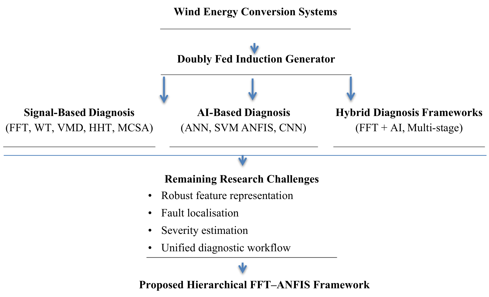
Figure 1. Evolution of DFIG ITSC fault-diagnosis approaches and positioning of the proposed hierarchical framework.
Algorithms 19 00718 g001
Figure 2. The topology of the DFIG-based WECS.
Algorithms 19 00718 g002
Figure 3. The three stator windings of a doubly fed induction generator with SC between turns in phase (a).
Algorithms 19 00718 g003
Figure 4. The block diagram of the proposed surveillance system for monitoring the state of DFIG.
Algorithms 19 00718 g004
Figure 5. Simulation result of healthy operation of DFIG: (a) Three-phase stator currents, (b) stator current phase ‘a’, and (c) the stator current spectrum in phase ‘a’.
Algorithms 19 00718 g005
Figure 6. Simulation results of DFIG operation under stator short-circuit (S_SC): (a) Three-phase stator currents, (b) stator current phase ‘a’, and (c) the stator current spectrum in phase ‘a’.
Algorithms 19 00718 g006
Figure 7. Simulation results of DFIG operation under rotor short circuit (R_SC): (a) Three-phase stator currents, (b) stator current phase ‘a’, and (c) the stator current spectrum in phase ‘a’.
Algorithms 19 00718 g007
Figure 8. Architecture of the neuro-fuzzy network.
Algorithms 19 00718 g008
Figure 9. (a) ANFIS training and validation RMSE; (b) actual vs. predicted outputs (test data); (c) prediction-error distribution; (d) ANFIS confusion matrix.
Algorithms 19 00718 g009
Figure 10. Sensitivity of the ANFIS fault classifier to input-feature perturbations: (a) classification accuracy under input-feature perturbations; (b) RMSE under input-feature perturbations. B. Sensitivity analysis of the ANFIS classifier.
Algorithms 19 00718 g010
Figure 11. Robustness analysis of the proposed ANFIS diagnostic framework under increasing measurement perturbations: (a) classification accuracy and (b) prediction RMSE.
Algorithms 19 00718 g011
Figure 12. (a) ANFIS training and validation RMSE; (b) actual vs. predicted outputs (test data); (c) prediction-error distribution; (d) ANFIS confusion matrix.
Algorithms 19 00718 g012
Figure 13. Sensitivity and robustness analysis of Model_2: (a) baseline confusion matrix, (b) classification accuracy, (c) RMSE, and (d) MAE under individual input-feature perturbations.
Algorithms 19 00718 g013
Figure 14. Robustness analysis of the proposed ANFIS-based stator-fault severity estimator under measurement noise: (a) mean classification accuracy, (b) mean RMSE, and (c) mean MAE.
Algorithms 19 00718 g014
Figure 15. Performance evaluation of the proposed ANFIS model for rotor-fault severity estimation: (a) RMSE, (b) Rotor fault severity, (c) Prediction error, (d) True Class, and (e) Probability density.
Algorithms 19 00718 g015
Figure 16. Sensitivity and robustness analysis of Model_3 under spectral-feature perturbations: (a) RMSE, (b) Severity classification accuracy, (c) R2, (d) Macro-F1, (e) ∆RMSE, (f) Sensitivity score, (g) Sensitivity score, (h) Maximum clipped samples, (i) Error, and (j) Minimum accuracy.
Algorithms 19 00718 g016
Figure 17. Robustness analysis of Model_3 under Gaussian feature perturbation: (a) mean classification accuracy, (b) mean RMSE, and (c) out-of-range input rate.
Algorithms 19 00718 g017
Figure 18. Validation test of resultants. (a) Healthy state; (b) S_SC faults (5%); (c) S_SC faults (20%); (d) R_SC faults (10%); (e) R_SC faults (15%); (f) M_SC faults (S_SC faults (15%) and R_SC faults (20%)); (g) M_SC faults (S_SC faults (5%) and R_SC faults (5%)); (h) M_SC faults (S_SC faults (15%) and R_SC faults (15%)).
Algorithms 19 00718 g018aAlgorithms 19 00718 g018b
Table 1. Comparative assessment of existing ITSC fault diagnosis methods and the main contributions of the proposed FFT–ANFIS framework comparative assessment of existing ITSC fault diagnosis methods and the main contributions of the proposed FFT–ANFIS framework.
Ref.Main ObjectiveMethodology/Main FeaturesFault/System ScopeDetectionFault LocalizationSeverity AssessmentValidationMain Limitations/Research GapDifference and Contribution of the Proposed FFT–ANFIS Method
Ma et al. (2021) [46]To mitigate the impact of ITSC faults on DFIG-based wind farms and maintain wind-farm power capability under faulty conditions.ITSC fault ride-through (FRT), turbine derating, and Particle Swarm Optimization (PSO)-based active-power dispatch.DFIG wind farm; stator ITSCIndirect/system-level, mainly for fault operation and mitigation rather than detailed diagnostic classification.Not addressed as a diagnostic task.Not addressed.MATLAB/Simulink-based simulation of wind-farm operation under ITSC.Focuses primarily on fault-tolerant operation and power optimization, rather than condition monitoring, fault localization, or quantitative severity diagnosis.The proposed method shifts the focus from fault mitigation and power dispatch to intelligent fault diagnosis. It provides a structured three-stage diagnostic capability—detection, localization, and severity assessment—using FFT spectral signatures and hierarchical ANFIS.
Aziz et al. (2026) [47]To detect, discriminate, and localize DFIG rotor-winding faults, particularly ITSC and high-resistance connection (HRC) faults.Three-layer ZSC–CASI–CADI framework using rotor zero-sequence current, Cosine Angle Spread Indicator, and Current Angle Difference Indicator.DFIG rotor winding; ITSC and HRCYes, using ZSC magnitude.Yes, using CADI to identify the faulty rotor phase.Limited/not a dedicated quantitative severity estimator; the framework primarily targets detection, discrimination, and phase localization.Extensive MATLAB/Simulink simulations under different load and rotor-speed conditions, including sub- and super-synchronous operation.Relies on zero-sequence current signatures and manually defined indicators; quantitative fault-severity estimation is not the central objective. The authors also identify future needs for adaptive thresholds, signal conditioning, and faster hardware implementation.The proposed FFT–ANFIS framework provides a data-driven nonlinear decision architecture rather than a sequence of analytically defined ZSC indicators. More importantly, it explicitly incorporates fault-severity assessment in addition to detection and localization, providing a broader diagnostic output.
Sayahi et al. (2025) [48]To diagnose stator ITSC faults and maintain DFIG operation through fault-tolerant control.DFIG state-space model, Takagi–Sugeno fuzzy model, Unknown Input Observer (UIO), Proportional–Integral Observer (PIO), and fault-tolerant controller.DFIG stator ITSCYes, through observer-based fault estimation.Fault isolation is addressed at the system/model level.Yes, fault level is estimated through the observer.Simulation of a 3 kW DFIG wind turbine.The principal contribution is fault estimation combined with fault-tolerant control, rather than a lightweight signal-based diagnostic architecture. It requires a model-based observer/controller framework and does not exploit frequency-domain current signatures through FFT.The proposed method offers a simpler signal-processing/AI diagnostic route, avoiding the need for an explicit UIO/T-S state-space observer and fault-tolerant controller. FFT extracts physically meaningful harmonic features, while hierarchical ANFIS performs the diagnostic decision and severity estimation.
Yu et al. (2020) [49]To detect faults in a DFIG using rotor-current information, while avoiding the need for a mechanical speed sensor.A new sliding mode observer (SMO) is developed from the mathematical model of the DFIG.The observer estimates rotor current and rotational speed.SMO-based residual detection using the difference between measured and estimated rotor currents.Limited/indirect: Mainly detects fault occurrence using rotor-current residuals; no dedicated quantitative fault-location estimation.Fault detection is then achieved by comparing the measured rotor current with the estimated rotor current.Simulation-based validation (MATLAB/Simulink).Mainly focused on model-based fault detection; limited capability for explicit fault localization and quantitative severity assessment; dependence on DFIG model accuracy and observer tuning; limited exploitation of frequency-domain fault signatures; and limited experimental validation.The proposed method offers a simpler signal-processing/AI diagnostic route, avoiding the need for an explicit DFIG model and SMO. FFT extracts physically meaningful harmonic features, while hierarchical ANFIS performs fault detection, localization, and severity assessment, extending Yu et al.’s observer-based fault detection toward comprehensive inter-turn fault diagnosis.
Bebars et al. (2022) [50]To systematically review internal electrical-fault detection techniques in DFIG-based wind turbines and identify advantages, limitations, and research gaps.Comprehensive review of model-based, signal-based, current-spectrum, wavelet, and other condition-monitoring techniques.DFIG stator and rotor internal electrical faultsReviews multiple approaches.Reviews multiple approaches.Identifies severity assessment as an important diagnostic requirement.Literature-based review covering more than 120 publications.A review paper rather than a new diagnostic algorithm; it highlights the need for high detection accuracy, early detection, and low computational burden.The proposed work directly addresses these identified requirements by developing a low-complexity hierarchical diagnostic framework based on FFT spectral features and ANFIS, with integrated detection, localization, and severity assessment.
Rengifo et al. (2024) [51]To detect and diagnose incipient ITSC faults and identify the affected phase in induction motors using machine-learning classifiers.Stator-current space-vector magnitude indicators combined with RF, SVM, kNN, FNN, and RNN classifiers; comparison with DWT-based indicators.Three-phase squirrel-cage induction motor, not DFIG.YesYes, affected phase identification.Primarily classification of fault states; quantitative severity estimation is not the central contribution.Experimental data from an induction motor.The methodology is developed for conventional induction motors rather than DFIGs; therefore, it does not directly account for DFIG-specific rotor-side dynamics, converter interaction, or variable-speed operation.The proposed method is specifically developed for DFIG-based wind-energy systems and exploits FFT harmonic features with ANFIS. Unlike the multi-classifier comparison in Rengifo et al., the proposed hierarchical structure integrates the diagnostic tasks into a single interpretable decision framework and explicitly targets fault-severity assessment.
Mohamed et al. (2021) [52]To diagnose combined ITSC and broken-rotor-bar faults using ANFIS.DWT-based feature extraction + ANFIS; comparison with conventional ANFIS and ANFIS using an autoregressive model.Squirrel-cage induction motor; combined ITSC and BRB faultsYesFault-state classification; detailed DFIG winding localization is not the focus.Mainly fault-state classification rather than explicit quantitative severity estimation.Experimental tests on a 1.5 hp, 380 V three-phase induction motor under different loads.Although it demonstrates the effectiveness of ANFIS, it concerns a squirrel-cage induction motor, uses DWT rather than FFT, and does not establish a hierarchical DFIG-specific framework for detection, localization, and severity assessment.The proposed work transfers the advantages of ANFIS-based intelligent diagnosis to the substantially more complex DFIG wind-generator environment, while replacing DWT with FFT-based spectral feature extraction and introducing a hierarchical diagnostic architecture that explicitly separates detection, localization, and severity assessment.
Table 2. WCES parameters.
Turbine parameters
Rated powerTurbine parameters
Air densityPn = 10 kW
Diameter of a bladeρ = 1.22 Kg/m3
Multiplier gainD = 3
Turbine moment of inertiaG = 5.4
Viscous coefficient of frictionJturbine = 0.042 kg.m2
DFIG parameters
Rated powerDFIG parameters
Rated speedPn = 7500 W
Supply voltageSn = 150 rad/s
Supply voltage frequencyVs = 220/380 V
Number of pole pairsfs = 50 Hz
Stator resistancep = 2
Rotor resistanceRs = 0.455 Ω
Mutual inductanceRr = 0.62 Ω
Cyclic stator inductanceMsr = 0.078 H
Cyclic rotor inductanceLs = 0.084 H
Coefficient of frictionLr = 0.081 H
Moment of inertiafg = 6.73 ∗ 10−3
DC bus parameters
DC bus voltageVDC = 800 V
DC bus capacityC = 2 × 10⁻³ F
Filter parameters
Resistance of the filterRf = 0.25 Ω
Inductance of the filterLf = 0.01 H
Table 3. Robustness performance of the ANFIS diagnostic model under random input perturbations.
PerturbationMean Accuracy (%)Std. Accuracy (%)Mean RMSEStd. RMSEAccuracy
Degradation (pp)
0%100.000.000.01520.00000.00
1%61.857.361.08850.146138.15
3%45.978.053.20470.482254.03
5%43.007.935.49100.761157.00
10%38.946.8011.06211.706261.06
20%39.977.4921.18773.277560.03
Table 4. Quantitative comparison of the proposed ANFIS with SVM and Random Forest.
MethodAccuracy (%)Macro-PrecisionMacro-RecallMacro-F1Balanced AccuracyRMSETraining Time (s)Inference Time (ms/Sample)
Proposed ANFIS100.001.00001.00001.00001.00000.01524.29543.8759
SVM90.910.97120.85000.87760.85000.60302.65339.9365
Random Forest100.001.00001.00001.00001.00000.00001.97168.4906
Table 5. Robustness performance of Model_2 under measurement noise.
Noise Level
(%)
Mean Accuracy
(%)
Mean RMSEMean MAEAccuracy
Degradation (pp)
0100.000.011010.007500.00
199.480.584350.390460.52
390.791.766851.172969.21
577.483.052402.0020022.52
1056.675.588993.8433643.33
2040.4510.819017.3474859.55
Table 6. Quantitative comparison of the proposed ANFIS with SVR and Random Forest Regression for stator-fault severity estimation.
Performance MetricProposed ANFISSVRRandom Forest
RMSE (%)0.01101.43382.2847
MAE (%)0.00751.34041.9278
R20.9999970.9492920.871250
MAPE (%)0.102816.269726.0268
Severity Accuracy (%)100.0096.9751.52
Macro-F11.00000.96910.4648
Training Time (s)2.43690.21280.7062
Inference Time (ms/sample)0.04170.28441.7081
Table 7. Robustness performance of Model_3 under Gaussian measurement noise.
Noise Level
(%)
Mean
Accuracy (%)
Mean
RMSE
Mean
MAE
Mean R2Accuracy
Degradation (pp)
Out-of-Range
Samples (%)
0100.000.0162280.0087900.9999940.000.00
198.760.7985450.5202850.9860161.2415.15
385.392.4949191.6083550.86483014.6115.48
573.644.1125472.6378940.62304426.3616.03
1057.457.7776415.096985−0.33580642.5517.03
2042.3313.4463449.228069−2.90709357.6719.24
Table 8. Quantitative comparison of the proposed ANFIS, SVR, and Random Forest for rotor-fault severity estimation.
Performance MetricProposed ANFISSVRRandom Forest
RMSE (%)0.0162281.0903983.157485
MAE (%)0.0087900.6712552.072381
R20.9999940.9749800.790203
MAPE (%)0.0675865.78868815.476083
Severity Accuracy (%)100.0093.9484.85
Macro-F11.00000.91430.7357
Training Time (s)3.0171802.1063482.817974
Prediction Time (s)0.6469200.1633330.214515
Table 9. Computational cost of the proposed hierarchical FFT–ANFIS models.
ModelModel_1Model_2Model_3
TaskFault ClassificationStator Severity RegressionRotor Severity Regression
Number of inputs555
Fuzzy rules5911
Total parameters80144176
Training time (s)0.90442.43692.7218
Inference time/sample (ms)0.015470.023910.02633
Memory footprint (MB)0.08710.14680.1766
Table 10. Comparative performance of fault diagnosis methods.
MethodStator Fault
Accuracy (%)
Rotor Fault Accuracy (%)MSC Accuracy (%)Computational Time (s)
Adaptive Observer
[74]
Not explicitly quantified; however, faults were effectively detected and simulated for γ = 5%High
(exact value not given)
Not covered in this studyFocus on the control strategy rather than speed
STFT + WPEDL
[79]
99.60%, and 99.52%
(current and vibration signal)
99.10%, and 99.50%
(current and vibration signal)
Not covered in this studyNot specified
VMD + RCMDE
[80]
High (exact value not given)High
(exact value not given)
Not covered in this studyNot specified
ECOC-SVM
[81]
94%Not applicableNot covered in this studyComputationally simple and
efficient
FFT
[82]
High (exact value not given)High
(exact value not given)
Not covered in this studyNot specified,
low computational complexity
ZSC
[83]
Not covered in this studyHigh (fault detection was successful at a low severity level (µ = 0.05))Not covered in this studyNot specified (low computational complexity).
Spectral, wavelet, and ratio computation analyses
[84]
Not covered in this studyNot given as a percentage, but the method reliably detects faults with increasing severity levelsNot covered in this study0.5 s
VMD-HHT-CNN [85]98.8%Not covered in this studyNot covered in this studyNot explicitly quantified, but the method is described as computationally efficient and lighter than EMD
TS-PI Observer
[86]
Not provided as a percentage, but the short-circuit fraction (μ) was accurately estimated using a PI observerNot covered in this studyNot covered in this studyNot explicitly mentioned, but the method is described as real-time capable and effective under varying wind and system parameters
Fault Ride-Through
[87]
The ITSC fault is reliably detected using a Luenberger observer and effectively mitigatedNot covered in this studyNot covered in this studyFast, real-time capable, and practically feasible
CEEMD-LSTM
[88]
95%Not covered in this studyNot covered in this studyLow-complexity and fast
ANFIS-FFT100%100%100%Fast, real-time capable, and practically feasible
Disclaimer/Publisher’s Note: The statements, opinions and data contained in all publications are solely those of the individual author(s) and contributor(s) and not of MDPI and/or the editor(s). MDPI and/or the editor(s) disclaim responsibility for any injury to people or property resulting from any ideas, methods, instructions or products referred to in the content.