Article

PSO-FSPMiner: A Metaheuristic Approach for Mining a Representative Subset of Frequent Similar Patterns


by
Ansel Y. Rodríguez-González
1,2,*,
Rosa María Valdovinos-Rosas
3,
Gretel Bernal Baró
3,
Ramón Aranda
2,4,
Angel Díaz-Pacheco
5 and
Miguel Á. Álvarez-Carmona
2,6
1
Unidad Académica Tepic, Centro de Investigación Científica y de Educación Superior de Ensenada, Tepic 63173, Mexico
2
Secretaría de Ciencia, Humanidades, Tecnología e Innovación, Ciudad de México 03940, Mexico
3
Campus Toluca, Universidad Autónoma del Estado de México, Toluca 50000, Mexico
4
Centro de Investigación en Matemáticas, Sede Mérida, Mérida 97302, Mexico
5
Campus Irapuato-Salamanca, Universidad de Guanajuato, Salamanca 36885, Mexico
6
Centro de Investigación en Matemáticas, Sede Monterrey, Monterrey 66629, Mexico
*
Author to whom correspondence should be addressed.
Algorithms 2026, 19(3), 229; https://doi.org/10.3390/a19030229
Submission received: 30 January 2026 / Revised: 6 March 2026 / Accepted: 13 March 2026 / Published: 18 March 2026

Abstract

In recent years, algorithms employing similarity functions beyond equality to unveil hidden knowledge have surged in popularity. Nonetheless, a notable challenge accompanying these algorithms is the proliferation of numerous frequent similar patterns, leading to heightened computational overhead and complicating analysis for humans. This paper proposes a metaheuristic approach based on Particle Swarm Optimization (PSO-FSPMiner) that extracts a representative subset of patterns to tackle this issue. Our experiments on real-world datasets demonstrate that the subset of frequent similar patterns mined by PSO-FSPMiner captures approximately 86.4% of the dataset’s knowledge, with a substantial reduction in frequent similar patterns of around 85.9%.

1. Introduction

Frequent pattern mining is one of the fundamental descriptive strategies in data mining, encompassing tasks such as association rule mining and clustering [1,2,3]. These approaches traditionally rely on strict equality when determining pattern occurrences. However, in many real-world domains, objects are rarely exactly identical, and similarity between attribute values is often approximate rather than exact.
To address this limitation, several research efforts have explored similarity-aware and approximate pattern mining. Recent studies have investigated the impact of different similarity measures in closed frequent pattern mining and analyzed their computational implications [4]. Approximate pattern mining has also been proposed in graph databases, allowing structural deviations during pattern matching [5]. In sequential and behavioral data analysis, item similarity has been incorporated through generalized pattern mining strategies aimed at reducing redundancy and improving interpretability [6]. These contributions highlight the increasing interest in relaxing exact matching requirements in pattern discovery.
Within this line of research, Frequent Similar Pattern (FSP) mining [7,8,9] extends traditional frequent pattern mining by explicitly incorporating similarity functions into the frequency computation, allowing occurrences of similar object descriptions to contribute to the frequency of a pattern. A frequent similar pattern is defined as a combination of feature values whose accumulated similarity across the dataset is greater than or equal to a user-specified threshold. Given a similarity function and a minimum frequency threshold, the goal of FSP mining is to identify all such patterns in an object description dataset.
Similarity functions [10,11,12] are widely used in exact, natural, and social sciences to compare objects beyond strict equality. Remarkable examples include applications in medicine [13,14], psychology [15], sociology [16], geology [17], and bioinformatics [18]. Through a similarity function, sub-descriptions of objects can be compared, and the frequency of both exact and similar sub-descriptions can be accumulated to detect regularities and support decision-making.
Several algorithms have been proposed for mining FSPs, including ObjectMiner [19], STree-based approaches [7,8], RP-Miner [20], and X-FSPMiner [9]. Although these algorithms enable the discovery of patterns that cannot be detected using traditional frequent pattern mining approaches [21,22,23,24,25,26], they typically generate an excessively large number of patterns, which increases both computational cost and analytical complexity.
A natural strategy to mitigate this issue is to identify a representative subset of FSPs. Bio-inspired optimization algorithms have traditionally addressed problems characterized by enormous search spaces. Particle Swarm Optimization (PSO) [27,28] is particularly attractive due to its simplicity and effectiveness and has been successfully applied to feature selection [29,30], hyper-parameter optimization [31], and association rule mining [32].
In this paper, we propose PSO-FSPMiner, a PSO-based metaheuristic designed to extract a representative subset of FSPs. The proposed approach introduces two evaluation functions—representativeness and coverage—to assess the quality of candidate pattern subsets. Representativeness evaluates shared attributes among patterns, while coverage measures the proportion of dataset instances described by the selected subset. Experimental results show that the subset mined by PSO-FSPMiner captures approximately 86.4% of the dataset’s knowledge while reducing the number of patterns by around 85.9%.
This paper is organized as follows. In Section 2, related work is reviewed. Section 3 provides the basic concepts related to FSP mining. Section 4 describes the proposed PSO-FSPMiner metaheuristic. Section 5 presents the experimental results and discussion. Finally, Section 6 includes the main concluding remarks and future work.

2. Related Work

Several research directions have explored the incorporation of similarity into pattern discovery. These approaches include approximate frequent pattern mining, similarity-aware pattern matching, and generalized pattern mining strategies that relax the strict equality assumption traditionally used in frequent pattern mining. Within this context, Frequent Similar Pattern (FSP) mining focuses specifically on incorporating similarity functions into the frequency computation process to accumulate occurrences of both exact and similar sub-descriptions.
Algorithms for FSP mining share the following aspects [7,8,19,20]: (i) For each attribute in the dataset, it is necessary to define a comparison criterion, which indicates the degree of similarity between the values compared. (ii) For each problem, a similarity function between patterns must be defined to determine the degree of similarity between them.
Taking into account the above criteria, the algorithms are classified considering the values returned by the similarity functions used and their monotony. A similarity function can be either Boolean or non-Boolean. A Boolean similarity function returns the values 0 or 1, i.e., the compared patterns will be considered similar or not by the mining process (ObjectMiner [19], STreeDC-Miner [7], RP-Miner [20], STreeNDC-Miner [7], X-FSPMiner [9]). On the other hand, a non-Boolean similarity function is one whose values are in the interval [0, 1]; i.e., the patterns will be similar to a greater or lesser extent depending on the value returned by the similarity function. Values close to 1 indicate a higher degree of similarity between patterns (STree*DC-Miner [8], STree*NDCMiner [8], and RP*-Miner [8]).
The monotonicity of similarity functions can be either non-increasing or increasing. A similarity function is non-increasing monotonic if and only if, for any pair of instances, the similarity concerning a set of attributes is greater than or equal to the similarity concerning any attributes superset. Deriving from the above, a new property is defined, called the f S -downward closure property, which states that all supersets of a non-frequent similar pattern are non-frequent [7], allowing the pruning of the FSPs search space [7,8]. Algorithms that use this type of functions are ObjectMiner [19], STreeDC-Miner [7], STree * DC-Miner [8], and X-FSPMiner [9]. Otherwise, when the similarity function is increasing, it does not satisfy the f S -downward closure property. The main FSPs mining algorithms that use this type of functions are STreeNDC-Miner [7], RP-Miner [20], STree * NDCMiner [8], and RP * -Miner [8].
The proposal in this paper aims to mine a representative subset of FSPs, using non-increasing monotonic and Boolean similarity functions. The main algorithms in the literature that find all FSPs for this type of similarity function are ObjectMiner, STreeDC-Miner, and X-FSPMiner. Therefore, in this section, we will focus exclusively on these algorithms.
ObjectMiner is based on the Apriori algorithm [33]. In the ObjectMiner [19] algorithm, we first identify frequent patterns for a single attribute value k. Next, we combine the frequent patterns from the previous iteration to create new candidate patterns of size k + 1 . We then determine which of the newly generated candidate patterns are FSPs. For each FSP, we calculate its frequency using a similarity function and iterate only over instances that contain patterns similar to the analyzed FSP. If the frequency is higher than the minimum frequency threshold, the candidate is considered an FSP. ObjectMiner continues until no FSP of size k is found. One major drawback of this algorithm is its high computational cost during the FSP mining process, as it does not take advantage of the potential repetition of patterns in the dataset.
The STreeDC-Miner [7] algorithm was proposed as an alternative to the main disadvantage of ObjectMiner. In STreeDC-Miner, similar patterns are grouped so as not to compare equal patterns. In addition, a tree structure called STree is created. For each attribute set A, a tree structure is generated, S T r e e A . Each leaf in the S T r e e A represents a pattern against the A attribute set and stores all repetitions and similar patterns in it. STreeDC-Miner, at each iteration, adds to the attribute set A a new attribute. In addition, at each iteration, the tree structure S T r e e A , corresponding to the existing attribute set in A, is constructed, the frequency of the patterns in S T r e e A is calculated, and the FSPs are obtained. The algorithm terminates when there are no frequent patterns for the attribute set A, or there are no attributes to add. During the STree construction, the similarity between two patterns is calculated only if their patterns in the previous recursive call are similar. Consequently, the number of evaluations of the similarity function is reduced, and the computational effort to compute the frequency of each pattern is also reduced. Therefore, the performance of the STreeDC-Miner outperforms the performance of the ObjectMiner [7].
X-FSPMiner [9] addresses the primary weakness of STreeDC-Miner, which involves constructing numerous tree structures (one for each attribute set) during the addition of new attributes. Drawing inspiration from the FP-Tree [34] and the PPC-Tree [35], X-FSPMiner employs a single tree structure, the FV-Tree, to condense the dataset. X-FSPMiner traverses the search space of Frequent Similar Patterns by starting with the subtrees of the FV-Tree that represent frequent similar patterns with only one attribute (the leaves) and expanding them by adding new attributes. This is done by exploring the immediate subtrees that contain these subtrees. The process continues until it reaches the root. Each possible expansion generated is therefore a valid expansion within the dataset, eliminating the need for candidate expansion generation and filtering. Additionally, only non-prunable feature values (those that are frequent patterns or similar to frequent patterns) are added. This reduces the number of candidates for frequent similar patterns since if the new feature value forms a prunable pattern, the expanded pattern will be prunable as well. The performance of X-FSPMiner significantly surpasses that of STreeDC-Miner and ObjectMiner.
Since X-FSPMiner, STreeDC-Miner, and ObjectMiner all extract the same set of FSPs, and the goal of this work is to identify a subset of representative FSPs, we use the X-FSPMiner algorithm to mine the complete set of FSPs. This set is then used to evaluate the quality of the subset of representative FSPs identified by the approach proposed in this work.

3. Basic Concepts and Notation

In this section, basic concepts and notation of FSP mining used in this paper are introduced, following the notations and definitions reported by [7].
Let Ω = { O 1 , O 2 , , O n } be a collection of instances that belong to the Ω dataset, O i Ω , 1 i n . Each instance O i is described by a set of attributes R = { r 1 , r 2 , , r m } and represented as a tuple ( v 1 , v 2 , , v m ) where v i D i , and D i is the domain of the values of attribute r i , 1 i m . A pattern of an instance O i for a subset of attributes S, S R , denoted by I S ( O ) , is a subdescription of O in terms of the attributes in S. Moreover, O [ r i ] is the value of the i-th attribute r ( r R ) in the O instance.
Given two patterns I S ( O ) and I S ( O ) O , O Ω , and a Boolean similarity function f S , defined as f S ( O , O ) = 1 whenever O is similar to O in terms of the attributes in S. On the other hand, f S ( O , O ) = 0 whenever O is not similar to O in terms of the attributes in S. An example of a Boolean similarity function is shown in Equation (1):
f S ( O , O ) = 1 if r S , C r ( O [ r ] , O [ r ] ) = 1 0 otherwise
where C r is a comparison criterion for the values of the r attribute. Some of the most commonly used comparison criteria are:
C r ( x , y ) = 1 if | x y | ε 0 otherwise
C r ( x , y ) = 1   if x = y 0   otherwise
Definition 1.
Let S be the subset of attributes S R , S , O Ω , and f S a Boolean similarity function; we define the frequency of a pattern I S ( O ) in Ω for f S as
F r e q u e n c y ( I S ( O ) ) = O Ω f S ( I S ( O ) , I S ( O ) )
According to the frequency definition, I S ( O ) is an FSP in Ω only if F r e q u e n c y ( I S ( O ) ) m i n F r e q , a minimum frequency threshold (usually set by the user). To prune the search space, an f S -downward closure is used [7].
Property 1
( f S -downward closure). Given a dataset Ω and a Boolean similarity function f S , f S fulfills the f S -downward closure if O , S 1 , S 2 ; O Ω ; S 1 S 2 R   [ F r e q u e n c y ( I S 1 ( O ) ) < m i n F r e q ] [ F r e q u e n c y ( I S 2 ( O ) )   < m i n F r e q ] .
The f S -downward closure does not always hold. The fulfillment of this property depends on the monotonicity of the frequency, which depends on the monotonicity of the similarity function [7].
Property 2
(Monotony of the frequency). Given a collection of instances Ω and a Boolean similarity function f S , f S satisfies frequency monotonicity if and only if O , S 1 , S 2 ; O Ω [ S 1 S 2 R ] [ F r e q u e n c y ( I S 1 ( O ) ) F r e q u e n c y ( I S 2 ( O ) ) ] .
Definition 2
(Monotonic similarity function). Given a collection of instances Ω and a Boolean similarity function f S , f S is non-increasing monotone O , O , S 1 , S 2 ; O , O Ω , [ S 1 S 2 R ] [ f S 1 ( O , O ) f S 2 ( O , O ) ] .
In this paper, we focus on mining a subset of FSPs using Boolean and non-increasing monotonic similarity functions.

4. Mining a Representative Subset of Frequent Similar Patterns

Particle Swarm Optimization (PSO) is a population-based metaheuristic inspired by the collective behavior observed in social systems and widely used for solving optimization problems [36]. In PSO, a set of candidate solutions, called particles, moves through the search space in order to find optimal or near-optimal solutions. Each particle is characterized by a position and a velocity, and its movement is influenced by two sources of information: its own best previously visited position (personal best, P B e s t ) and the best position found by any particle in the swarm (global best, G B e s t ).
At each iteration, the velocity and position of every particle are updated according to these two guiding solutions, allowing particles to explore the search space while gradually converging toward promising regions. Due to its simplicity and effectiveness, PSO has been successfully applied to a wide range of optimization problems in data mining and machine learning.
Inspired by this search strategy, we propose a novel algorithm named PSO-FSPMiner, designed to mine a representative subset of frequent similar patterns (FSPs). Starting from an initial random particle swarm, each particle moves through the search space, updating its position and velocity based on its best position and the global best solution. Each particle represents a candidate pattern. Patterns with higher frequency are considered better solutions.
In this work, PSO-FSPMiner is formulated as a metaheuristic approach because it uses a population-based stochastic search strategy to explore the large combinatorial space of possible pattern subsets without exhaustively enumerating all candidate solutions.
Our proposed algorithm includes mechanisms to update both numeric and non-numeric attributes. In addition, the most relevant solutions considering their representativeness and coverage of Ω are stored in an external list, which is updated in each iteration.
Details on how to measure the relevance of patterns and the PSO-FSPMiner algorithm are described in the following subsections.

4.1. Relevance Measures

The proposed PSO-FSPMiner algorithm considers two criteria: quality and relevance. In this sense, quality is measured in terms of frequency; more frequent patterns are considered to have higher quality, and a pattern is relevant if it is not redundant. For determining whether a pattern is redundant, two new functions are introduced, inspired by [37]: representativeness and coverage. Representativeness represents the proportion of common attributes between the compared patterns, and coverage measures the number of instances that add up to the frequency of both patterns. The following paragraphs formally describe both functions.
Definition 3.
Considering two instances O , O Ω , two sets of attributes S and S , and a non-increasing monotone Boolean similarity function f S . The representativeness between the patterns I S ( O ) , and I S ( O ) is obtained by
R p ( I S ( O ) , I S ( O ) ) = f S S ( I S ( O ) , I S ( O ) ) | S S | m i n ( | S | , | S | )
where f S S returns 0 or 1 depending on whether all the values of the common attributes between the patterns are similar, | S S | returns the number of common attributes between the patterns, and m i n ( | S | , | S | ) returns the minimum of the number of attributes existing between the patterns.
Representativeness values close to 0 reveal that two patterns are very different; otherwise, values equal to 1 mean that both patterns provide the same knowledge. However, even if the representativeness value equals 1, it is also necessary to examine the percentage of common instances that add up to the frequency of both patterns concerning the instances that add up to the frequency of the patterns I S ( O ) and I S ( O ) separately.
Definition 4.
Given two instances O , O Ω and two sets of attributes S and S , S, S R. We define the coverage between two patterns I S ( O ) and I S ( O ) as follows:
C o v ( I S ( O ) , I S ( O ) ) = M a x ( C ( I S ( O ) , I S ( O ) ) C ( I S ( O ) ) , C ( I S ( O ) , I S ( O ) ) C ( I S ( O ) ) )
C ( I S ( O ) , I S ( O ) ) = | { O Ω | f S S ( O , O ) = 1 Λ f S S ( O , O ) = 1 } |
C ( I S ( O ) ) = | { O Ω | f S ( O , O ) = 1 } |
where C ( I S ( O ) , I S ( O ) ) represents the number of common instances that sum to the frequency of both patterns I S ( O ) and I S ( O ) regarding attributes in S S . C ( I S ( O ) ) and C ( I S ( O ) ) represent the number of instances that contribute to the frequency of the patterns I S ( O ) and I S ( O ) respectively. The value returned by coverage can be interpreted as the maximum percentage of common instances covered by the patterns I S ( O ) and I S ( O ) .
Once the concepts of representativeness (Definition 1) and coverage (Definition 2) have been introduced, we define that
Definition 5.
Given two patterns I S ( O ) and I S ( O ) : if their representativeness value is equal to 1 and their coverage value is greater than the minimum coverage threshold (CovMin), then the patterns are considered redundant.
If two patterns are redundant, then the dominance between patterns must be analyzed, and the solution that provides the most information regarding the attributes present and the number of instances covered is retained. Therefore, a pattern I S ( O ) dominates another solution I S ( O ) if the following conditions are met: (i) I S ( O ) dominates I S ( O ) if the length of I S ( O ) is greater than the length of I S ( O ) ( | I S ( O ) | > | I S ( O ) | ). (ii) Otherwise, I S ( O ) dominates I S ( O ) if | I S ( O ) | = | I S ( O ) | and C ( I S ( O ) ) > C ( I S ( O ) ) .
In the first case, the I S ( O ) pattern is chosen because, in addition to the attribute values present in I S ( O ) , it has other non-common attribute values; therefore, it provides more knowledge of the dataset. In the second case, since both patterns have the same number of attribute values, the pattern with higher frequency is taken (because those patterns that cover a larger number of instances are considered more descriptive). A particular case is when the representativeness and coverage values are equal to 1, and the patterns cover exactly the same instances in the dataset. In that case, any of them could be selected.

4.2. PSO-FSPMiner

The PSO-FSPMiner algorithm receives as input parameters: the dataset Ω , the population size N, the number of iterations to be performed I t e r , the minimum frequency threshold m i n F r e q , the minimum coverage threshold m i n C o v , the inertial factor w, the acceleration constants c 1 and c 2 , and a weight variable called b o o s t W e i g h t (Algorithm 1).
In PSO-FSPMiner, like the traditional PSO algorithm [38], each solution in the search space represents a particle (similar pattern). P B e s t i is the best particle (frequently a similar pattern) found for the particle P i , and V i is the velocity at which the particle P i will move. Fitness ( P i ) represents the fitness value of the current particle P i , while F i t n e s s ( P B e s t i ) represents the fitness value of P B e s t i . G B e s t is the best particle (best FSP) found for all the particles, and F i t n e s s ( G B e s t ) represents the fitness value of G B e s t .
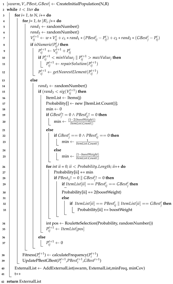
At the beginning, t = 0 , and the initial population of size N is randomly generated (line 1). Each particle P i of the population is represented as a vector of size | R | , where | R | represents the number of attributes existing in the dataset. At each position of the vector, the possible values correspond to the existing values in the analyzed attribute or 0 in case the attribute value is not included in the pattern. Each component of the initial velocity vector V i for the particle P i is initialized to 0. Each time a new particle is generated at iteration t, denoted as P i t , it is computed from Ω , and its F i t n e s s ( P i t ) is also updated (the fitness is measured in terms of the frequency).
After computing the fitness of each particle in the initial population, both the local best position P B e s t i t and F i t n e s s ( P B e s t i t ) are updated with the particle P i t and its fitness, respectively. In addition, the best solution, G B e s t , and its F i t n e s s ( G B e s t ) are updated with the best solution found so far. This proposal incorporates an external list in which the best solutions are stored. Thus, each time a new population is generated, the representativeness (by Equation (5)) and coverage (by Equation (6)) of each solution with respect to the existing solutions in the external list are calculated, and if it is not redundant, the analyzed solution is added to the external list. Otherwise, the dominant solution is selected. If the dominant solution belongs to the new population, the dominated solution is removed from the external list, and the new solution is inserted as shown in Algorithm 2.
While the number of iterations is not reached (line 2), the position of each particle (line 4) in the search space is updated. For this, it is necessary to update each component of the velocity vector by the following expression (line 7):
V i j t + 1 = w V i j t + c 1 r a n d 1 ( P B e s t i j t P i j t ) + c 2 r a n d 2 ( G B e s t j t P i j t )
where w is the inertial factor and represents the expected degree of similarity between the new velocity vector V t + 1 and the previous velocity vector V t . c 1 and c 2 are the acceleration constants, which are weights for giving more relevance to the best local position or the best global position. w, c 1 , and c 2 are parameters defined by the user. r a n d 1 and r a n d 2 are random values in the interval (0, 1).
To update the position of a particle P i t , each component of the position vector is analyzed, taking into account whether the attribute value in P i j t is numeric or non-numeric (line 8) Equation (10) or Equation (11) is used.
P i j t + 1 = P i j t + V i j t + 1
s i g ( V i j t + 1 ) = 1 1 + e V i j t + 1
Algorithm 1: PSO-FSPMiner algorithm
   Input: Dataset Ω, Population size N, Number of Iterations Iter, Min frequency threshold minFreq,
   Min coverage threshold minCov, Inertial factor w, acceleration constant c 1 , acceleration constant c 2 ,
   Weight variable boostWeight
   Output: Returns the set of existing solutions in the External List E x t e r n a l L i s t
Algorithms 19 00229 i001
If the value of the attribute in P i j t is numeric, P i j t is updated using Equation (10). Then we check if P i j t + 1 is outside the [minValuej,maxValuej] interval (line 10). minValuej and maxValuej correspond to the minimum and maximum values existing in the attribute at position j. If the condition is satisfied, solution P i j t + 1 is repaired (line 11). If P i j t + 1 is less than m i n V a l u e j , then P i j t + 1 is assigned the value of m i n V a l u e j . Otherwise, it is assigned the value of m a x V a l u e j . P i j t + 1 will always be assigned to the attribute value at position j closest to the value of P i j t + 1 (line 12). This guarantees that the value of P i j t + 1 is always an existing attribute value.
If the attribute value in P i j t is not numeric, V i j t + 1 is defined in terms of the probability that a value of an attribute j has of appearing in the pattern P i t + 1 . For this reason, the value of V i j t + 1 must be restricted within the range [0, 1]. The most commonly used normalization function is the sigmoid (Equation (11)) [39,40,41]. Then, a random value within the range [0, 1] is generated; if the generated random value is greater than s i g ( V i j t + 1 ) (line 15), it means that the attribute at position j is excluded from the solution P i t + 1 , P i j t + 1 = 0 (line 37). Otherwise, it is necessary to assign a probability of occurrence to each value of the attribute at j. Initially, this probability is the same for all values of the attribute at j and varies depending on whether or not P B e s t i t and G B e s t t have a value at that position.
Once the minimum probability value ( m i n ) is defined, it is assigned to each attribute’s value at j (line 27). If the attribute value coincides with the existing attribute value in P B e s t i j t and G B e s t j t (line 29), its probability will be higher by 2 times b o o s t W e i g h t . The b o o s t W e i g h t value is a parameter defined to give more weight to those values of attribute j existing in P B e s t i j t and G B e s t j t . In case the attribute value only matches one of the existing values in P B e s t i j t and G B e s t j t (line 32), its probability is going to be higher by b o o s t W e i g h t (line 33). Then, using the method of Selection by Roulette [42], we obtain a random number on the [0, 1] interval to assign it to P i j t + 1 (line 35).
Once the particle is updated, the fitness of the new position P i j t + 1 is calculated (line 38). If the new fitness is the best one found so far for the particle P i t + 1 , P B e s t i t + 1 and its fitness are updated. Similarly, if the new fitness is the best global solution found so far, G B e s t t + 1 and its fitness are updated (line 39). At each iteration, the new population ( s w a r m ) is checked for redundant solutions concerning the existing solutions in the external list ( E x t e r n a l L i s t ) (line 40) (See Algorithm 2), and the non-redundant solutions are added to the external list. The algorithm stops when the number of iterations ( I t e r ) is reached and returns the subset of existing solutions in the external list.
Algorithm 2: AddExternalList
   Input: Solutions swarm, External List ExternalList, Min Frequency minFreq, Min coverage minCov
   Output: Returns the list of non-redundant solutions
Algorithms 19 00229 i002
It is important to remark that, unlike exhaustive frequent similar pattern mining algorithms—which may exhibit exponential worst-case behavior due to the combinatorial enumeration of candidate patterns, even when pruning strategies based on the f S -downward closure property are employed—PSO-FSPMiner does not attempt to enumerate the complete pattern space. Instead, it performs a bounded stochastic search controlled by the swarm parameters. A detailed discussion of its computational characteristics is provided in Section 5.

5. Experiments and Results

In this section, the PSO-FSPMiner metaheuristic performance is evaluated. Table 1 gives a description of the two-class datasets taken from the UCI Machine Learning Repository (https://archive.ics.uci.edu/ml/index.php (accessed on 1 December 2025)) used in the experiments. For all datasets, a non-increasing monotonic Boolean similarity function was employed (Equation (1)). For each numerical attribute r, the comparison criterion used was the one obtained by Equation (2) with ε = α × ( m a x V m i n V ) , where m a x V is the maximum v D r , m i n V is the minimum v D r , and α = 0.05 . For non-numerical attributes, the comparison criterion adopted was obtained with Equation (3). The Imbalance column refers to the measure used to calculate the degree of class imbalance in the dataset [43].
The X-FSPMiner algorithm (the implementation of X-FSPMiner provided by its authors was used) is applied as a baseline method because it mines all FSPs in less time than other approaches in the state of the art. The FSP subset quality mined by PSO-FSPMiner was evaluated concerning the set of patterns returned by the X-FSPMiner algorithm. To assess the performance of PSO-FSPMiner in different scenarios, the frequency threshold was varied in the range of 0.02 to 0.10, with a step size of 0.02. Other free parameters were the population size = 100 particles, c 1 and c 2 were set to 1.74, the inertia w to 0.869, 100 iterations, and the variable of weight b o o s t W e i g h t was set at 0.1. In each run of the algorithm, for each subset, the quantity, quality, and the percentage that represents the total FSPs were measured.
The supervised K-Nearest-Neighbor (KNN) [44] classifier was used to evaluate the quality of the FSP subset mined. In this sense, the quality was measured taking into account the accuracy obtained by the KNN classifier when classifying all FSP (mined with the X-FSPMiner algorithm) using the subset mined by PSO-FSPMiner. The parameter k was set to 5.
Equation (12) corresponds to the distance metric used by the KNN classifier, and it returns the proportion of similar attributes between the patterns compared:
D i s t ( I S ( O ) , I S ( O ) ) = f S S ( I S ( O ) , I S ( O ) ) | S S | | S S |
Table 2 shows the FSP subset obtained. Each row contains the average values corresponding to 10 runs of the algorithm for each frequency threshold. The third and fourth columns show the number of patterns mined by the X-FSPMiner and PSO-FSPMiner algorithms respectively. Values in parentheses contain the standard deviation. The fifth column represents the ratio between the subset of patterns mined and the total of FSPs mined. The O A c c u r a c y column contains the overall accuracy.
The results of Table 2 can be analyzed in two ways: the quantity of FSPs and the quality of the subset of FSPs mined.
Concerning the amount of FSPs mined, it is possible to notice the reduction capacity of the PSO-FSPMiner with respect to the X-FSPMiner algorithm. A reduction up to 99% is achieved (in the Liver Disorders datasets for frequency threshold 0.02 (140 of 16,434 FSPs) and Indian Liver Patient for frequency threshold 0.06 (1298 of 165,608 FSPs)). Also, we can observe from Figure 1 that the number of patterns mined by PSO-FSPMiner was less than 20% in more than 80% of the test scenarios (41 of 50). It means a reduction of more than 80% of the amount of FSPs mined. The most significant reductions are seen in Liver Disorders, Indian Liver Patients, Credit Approval, Breast, Diagnosis, Cryotherapy, and Algerian datasets, where, for all tested frequency thresholds, the subset of patterns mined contains less than 15% of the whole FSPs mined by X-FSPMiner. It is relevant to mention that in the worst case, the reduction was more than 40% of the amount of FSPs mined, and on average, the reduction was 85.9%.
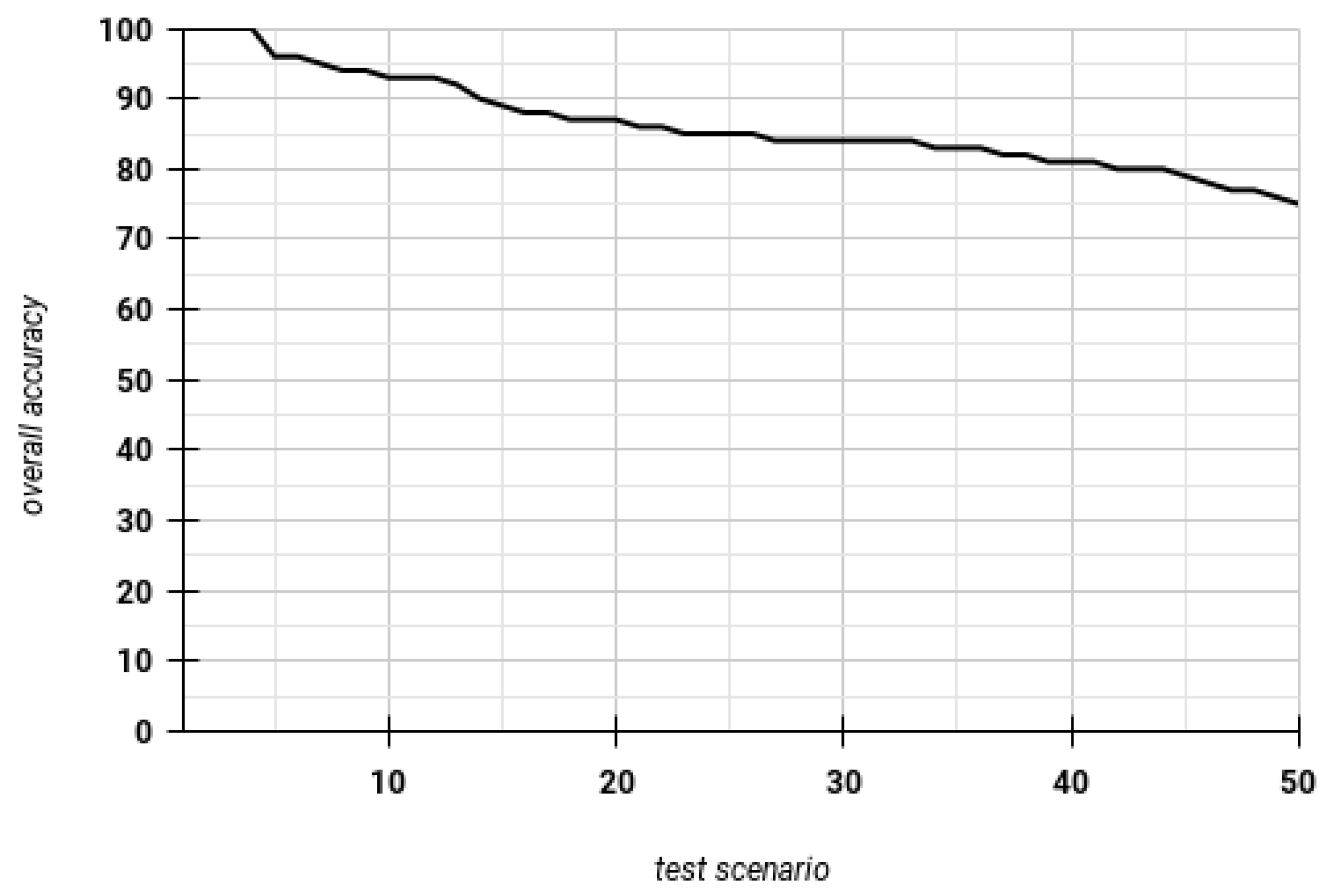
On the other hand, with respect to the quality of the subset of patterns mined by PSO-FSPMiner, in 100% of the cases, the overall accuracy was equal to or higher than 75%. The lowest accuracy value (75%) was obtained in the Liver Disorders dataset for a frequency threshold of 0.1. In the same way, the best PSO-FSPMiner behavior was obtained on the Glass dataset. Also, from Figure 2, we can observe that more than 80% of the existing FSPs can be correctly classified in more than 80% of the test scenarios (44 of 50). On average, our algorithm retains a general descriptive power above 86.4%.
To assess whether the observed differences in performance across the tested frequency thresholds are statistically significant, a non-parametric statistical analysis was conducted. Since the experiments involve multiple configurations evaluated across several datasets, we adopted the ranking-based comparison methodology commonly used for algorithm evaluation across multiple datasets [45]. First, the average ranks of the different frequency thresholds were computed across all experimental scenarios. Then, the Nemenyi post-hoc test was applied to determine whether the differences between these ranks were statistically significant. According to this test, two configurations are considered significantly different if the difference between their average ranks exceeds the critical difference (CD) value for the selected significance level.
To determine whether the quality of the subset of patterns varied significantly depending on the frequency threshold, we applied the Nemenyi post-hoc test [45]. Results of the Nemenyi tests for α = 0.05 are shown in Table 3, where each value represents the differences between the mean rank of each threshold, and the last row shows the critical difference.
From Table 3, it can be observed that none of the pairwise differences between the evaluated frequency thresholds exceeds the critical difference value. Therefore, no statistically significant differences were detected among the tested thresholds at the α = 0.05 significance level. This result indicates that the performance of PSO-FSPMiner remains stable across the evaluated frequency thresholds. Additionally, the accuracy values reported in Table 2 remain consistently above 75%, indicating that the proposed metaheuristic is able to identify compact subsets of high-quality patterns. By means of the designed objective functions, PSO-FSPMiner promotes the selection of representative patterns while reducing redundancy, retaining only those FSPs that provide complementary knowledge about the dataset.

Computational Performance and Resource Considerations

From a computational standpoint, PSO-FSPMiner differs fundamentally from exhaustive frequent similar pattern mining algorithms. Exhaustive approaches aim to enumerate the complete set of frequent patterns and may exhibit exponential worst-case behavior due to the combinatorial growth of candidate patterns, even when pruning strategies based on the f S -downward closure property are applied.
In contrast, PSO-FSPMiner does not attempt full pattern space enumeration. Instead, it conducts a population-based stochastic search guided by particle swarm optimization. For fixed swarm parameters (population size P and number of iterations T), the computational cost of PSO-FSPMiner is bounded by O ( P · T · N · m ) , where N denotes the number of objects and m the number of attributes. Each particle evaluation requires computing similarity-based support across the dataset, which scales linearly with respect to N and m. Therefore, the computational effort per execution is explicitly controlled by the swarm parameters and does not involve combinatorial enumeration of the full pattern space.
All experiments were executed on a workstation equipped with an Intel® Core i7 CPU at 1.80–2.00 GHz and 8 GB of RAM. Under these hardware constraints, all experimental runs were completed successfully without memory saturation or instability.
In practice, under the experimental configuration described in Section 5, each execution of PSO-FSPMiner (100 particles, 100 iterations) completed successfully for all evaluated datasets without excessive runtime growth or memory saturation, even in scenarios where the total number of FSPs exceeded 200,000.
It is important to emphasize that the objective of the proposed method is not to accelerate exhaustive enumeration but to identify a representative subset of frequent similar patterns. Consequently, direct runtime comparisons with algorithms designed for complete pattern extraction would not constitute a strictly equivalent evaluation framework, as the underlying computational goals differ substantially.
Although a detailed benchmarking study against exhaustive mining algorithms in terms of runtime and memory consumption was beyond the primary scope of this work, future research will include a systematic empirical comparison under standardized computational settings.

6. Concluding Remarks

Frequent Similar Pattern mining is emerging as an alternative solution in data mining to the traditional frequent pattern mining algorithms, revealing hidden knowledge. However, the existing algorithms for mining FSP obtain a large number of patterns. Their analysis is costly due to many patterns offering the same knowledge of the dataset. For this reason, in this work, a metaheuristic (PSO-FSPMiner) was developed for mining a subset of FSPs that describes the whole dataset.
The PSO-FSPMiner algorithm has the particularity that only those patterns that are considered relevant and not redundant are stored in the subset of solutions. In the same way, two new functions for evaluating the number of common attributes and the proportion of instances covered by the patterns analyzed were proposed (representativeness and coverage).
Our main contribution was the proposal of this new meta-heuristic that incorporates the two functions (representativeness and coverage) to mine a subset of patterns able to describe the whole dataset.
Experiments showed that our approach is able to significantly reduce the FPS rate (about 85.9%) while retaining a general descriptive power of about 86.4%. On the other hand, the results provided evidence of the stability of our approach. Their performance did not change significantly, regardless of the frequency threshold or the size of the data set; a smaller subset of patterns was obtained, avoiding redundant FSPs and keeping those with interesting knowledge.
In future work, different similarity functions, other than Boolean ones, will be explored in order to extend the applicability of our algorithm. Also, visualize developing a meta-heuristic based on the current proposal to mine a subset of association rules.

Author Contributions

Conceptualization, A.Y.R.-G. and R.M.V.-R.; methodology, A.Y.R.-G. and R.M.V.-R.; software, A.Y.R.-G. and G.B.B.; validation, A.D.-P., R.A. and M.Á.Á.-C.; formal analysis A.Y.R.-G. and G.B.B.; investigation, A.Y.R.-G. and G.B.B.; resources, A.Y.R.-G. and G.B.B.; data curation, G.B.B.; writing—original draft preparation, A.Y.R.-G., R.M.V.-R. and G.B.B.; writing—review and editing, A.D.-P., R.A., M.Á.Á.-C. and A.Y.R.-G.; visualization, A.Y.R.-G.; supervision, A.Y.R.-G. and R.M.V.-R. All authors have read and agreed to the published version of the manuscript.

Funding

This research received no external funding.

Institutional Review Board Statement

Not applicable.

Informed Consent Statement

Not applicable.

Data Availability Statement

The original contributions presented in this study are included in the article. Further inquiries can be directed to the corresponding author.

Conflicts of Interest

The authors declare no conflicts of interest.

Abbreviations

The following abbreviations are used in this manuscript:
FSPFrequent Similar Pattern
FSPsFrequent Similar Patterns
FSPMinerFrequent Similar Pattern Miner
PSOParticle Swarm Optimization
PSO-FSPMinerParticle Swarm Optimization-Frequent Similar Pattern Miner
STreeSimilarity Tree
FV-TreeFeature-Value Tree
FP-TreeFrequent Pattern Tree
PPC-TreePrePost Coding Tree
UCIUniversity of California, Irvine
KNNk-Nearest Neighbor

References

  1. Agrawal, R.; Imieliński, T.; Swami, A. Mining association rules between sets of items in large databases. In Proceedings of the 1993 ACM SIGMOD International Conference on Management of Data, Washington, DC, USA, 26–28 May 1993; pp. 207–216. [Google Scholar] [CrossRef]
  2. Fournier-Viger, P.; Gan, W.; Wu, Y.; Nouioua, M.; Song, W.; Truong, T.; Duong, H. Pattern Mining: Current Challenges and Opportunities. In Proceedings of the Database Systems for Advanced Applications. DASFAA 2022 International Workshops; Rage, U.K., Goyal, V., Reddy, P.K., Eds.; Springer: Cham, Switzerland, 2022; pp. 34–49. [Google Scholar] [CrossRef]
  3. Han, J.; Pei, J.; Tong, H. Data Mining: Concepts and Techniques; Morgan Kaufmann: Burlington, MA, USA, 2022. [Google Scholar]
  4. Cam, T.T.; Hung, D. Comparing Similarity Measures: Applications in Mining Frequent Closed Patterns. In Proceedings of the Data Analytics and Management; Swaroop, A., Virdee, B., Correia, S., Polkowski, Z., Eds.; Springer: Cham, Switzerland, 2026; pp. 503–519. [Google Scholar] [CrossRef]
  5. Driss, K.; Boulila, W.; Leborgne, A.; Gançarski, P. Mining frequent approximate patterns in large networks. Int. J. Imaging Syst. Technol. 2021, 31, 1265–1279. [Google Scholar] [CrossRef]
  6. Daher, J.B.; Brun, A. Handling Item Similarity in Behavioral Patterns through General Pattern Mining. In Proceedings of the 2020 IEEE/WIC/ACM International Joint Conference on Web Intelligence and Intelligent Agent Technology (WI-IAT), Melbourne, Australia, 14–17 December 2020; pp. 611–618. [Google Scholar] [CrossRef]
  7. Rodríguez-González, A.Y.; Martínez-Trinidad, J.F.; Carrasco-Ochoa, J.A.; Ruiz-Shulcloper, J. Mining frequent patterns and association rules using similarities. Expert Syst. Appl. 2013, 40, 6823–6836. [Google Scholar] [CrossRef]
  8. Rodríguez-González, A.Y.; Martínez-Trinidad, J.F.; Carrasco-Ochoa, J.A.; Ruiz-Shulcloper, J.; Alvarado-Mentado, M. Frequent similar pattern mining using non Boolean similarity functions. J. Intell. Fuzzy Syst. 2019, 36, 4931–4944. [Google Scholar] [CrossRef]
  9. Rodríguez-González, A.Y.; Aranda, R.; Álvarez Carmona, M.A.; Díaz-Pacheco, A.; Rosas, R.M.V. X-FSPMiner: A Novel Algorithm for Frequent Similar Pattern Mining. ACM Trans. Knowl. Discov. Data 2024, 18, 121. [Google Scholar] [CrossRef]
  10. Weisberg, M. Getting serious about similarity. Philos. Sci. 2012, 79, 785–794. [Google Scholar] [CrossRef]
  11. Cha, S.H. Comprehensive Survey on Distance/Similarity Measures between Probability Density Functions. Int. J. Math. Model. Methods Appl. Sci. 2007, 1, 300–307. [Google Scholar]
  12. Tversky, A. Features of similarity. Psychol. Rev. 1977, 84, 327. [Google Scholar] [CrossRef]
  13. Ortiz-Posadas, M.R. The Logical Combinatorial Approach Applied to Pattern Recognition in Medicine. In Proceedings of the New Trends and Advanced Methods in Interdisciplinary Mathematical Sciences; Toni, B., Ed.; Springer: Cham, Switzerland, 2017; pp. 169–188. [Google Scholar] [CrossRef]
  14. Alemán-García, N.; Ortiz-Posadas, M.R. Evaluation of Hepatic Fibrosis Stages Using the Logical Combinatorial Approach. In Proceedings of the Progress in Artificial Intelligence and Pattern Recognition; Hernández Heredia, Y., Milián Núñez, V., Ruiz Shulcloper, J., Eds.; Springer: Cham, Switzerland, 2021; pp. 158–166. [Google Scholar] [CrossRef]
  15. Medin, D.L.; Goldstone, R.L.; Gentner, D. Respects for similarity. Psychol. Rev. 1993, 100, 254. [Google Scholar] [CrossRef]
  16. Leicht, E.A.; Holme, P.; Newman, M.E.J. Vertex similarity in networks. Phys. Rev. E 2006, 73, 026120. [Google Scholar] [CrossRef] [PubMed]
  17. Cheng, Q. Mapping singularities with stream sediment geochemical data for prediction of undiscovered mineral deposits in Gejiu, Yunnan Province, China. Ore Geol. Rev. 2007, 32, 314–324. [Google Scholar] [CrossRef]
  18. Altschul, S.F.; Gish, W.; Miller, W.; Myers, E.W.; Lipman, D.J. Basic local alignment search tool. J. Mol. Biol. 1990, 215, 403–410. [Google Scholar] [CrossRef]
  19. Danger, R.; Ruíz-Shulcloper, J.; Llavori, R.B. Objectminer: A New Approach for Mining Complex Objects. In Proceedings of the ICEIS (2); Citeseer: University Park, PA, USA, 2004; pp. 42–47. [Google Scholar]
  20. Rodríguez-González, A.Y.; Martínez-Trinidad, J.F.; Carrasco-Ochoa, J.A.; Ruiz-Shulcloper, J. RP-Miner: A relaxed prune algorithm for frequent similar pattern mining. Knowl. Inf. Syst. 2011, 27, 451–471. [Google Scholar] [CrossRef]
  21. Li, L.; Ding, P.; Chen, H.; Wu, X. Frequent Pattern Mining in Big Social Graphs. IEEE Trans. Emerg. Top. Comput. Intell. 2021, 6, 638–648. [Google Scholar] [CrossRef]
  22. Patro, P.P.; Senapati, R. Advanced binary matrix-based frequent pattern mining algorithm. In Intelligent Systems; Springer: Berlin/Heidelberg, Germany, 2021; pp. 305–316. [Google Scholar] [CrossRef]
  23. Ruiz, E.; Casillas, J. Adaptive fuzzy partitions for evolving association rules in big data stream. Int. J. Approx. Reason. 2018, 93, 463–486. [Google Scholar] [CrossRef]
  24. Siahaan, A.P.U.; Ikhwan, A.; Aryza, S. A novelty of data mining for promoting education based on FP-growth algorithm. Int. J. Civ. Eng. Technol. 2018, 9, 1660–1669. [Google Scholar] [CrossRef]
  25. Zhang, C.; Tian, P.; Zhang, X.; Jiang, Z.L.; Yao, L.; Wang, X. Fast eclat algorithms based on minwise hashing for large scale transactions. IEEE Internet Things J. 2018, 6, 3948–3961. [Google Scholar] [CrossRef]
  26. Koppar, M.R.N.; Ramesh, D. Novel Algorithms for Maximal Frequent Pattern Mining. J. Optoelectron. Laser 2022, 41, 449–455. [Google Scholar] [CrossRef]
  27. Dey, A.; Bhattacharyya, S.; Dey, S.; Platos, J.; Snasel, V. Automatic clustering of colour images using quantum inspired meta-heuristic algorithms. Appl. Intell. 2023, 53, 9823–9845. [Google Scholar] [CrossRef]
  28. Chaffi, B.N.; Rahmani, M. A novel two-phase hybrid selection mechanism feeder to improve performance of many-objective optimization algorithms. Evol. Intell. 2022, 17, 889–920. [Google Scholar] [CrossRef]
  29. Abualigah, L.M.; Khader, A.T. Unsupervised text feature selection technique based on hybrid particle swarm optimization algorithm with genetic operators for the text clustering. J. Supercomput. 2017, 73, 4773–4795. [Google Scholar] [CrossRef]
  30. Abualigah, L.M.; Khader, A.T.; Hanandeh, E.S. A new feature selection method to improve the document clustering using particle swarm optimization algorithm. J. Comput. Sci. 2018, 25, 456–466. [Google Scholar] [CrossRef]
  31. Díaz-Pacheco, A.; Reyes-Garcia, C.A. A classification-based fuzzy-rules proxy model to assist in the full model selection problem in high volume datasets. J. Exp. Theor. Artif. Intell. 2022, 34, 815–844. [Google Scholar] [CrossRef]
  32. Li, G.; Wang, T.; Chen, Q.; Shao, P.; Xiong, N.; Vasilakos, A. A Survey on Particle Swarm Optimization for Association Rule Mining. Electronics 2022, 11, 3044. [Google Scholar] [CrossRef]
  33. Al-Maolegi, M.; Arkok, B. An improved Apriori algorithm for association rules. arXiv 2014, arXiv:1403.3948. [Google Scholar] [CrossRef]
  34. Grahne, G.; Zhu, J. Fast algorithms for frequent itemset mining using FP-trees. IEEE Trans. Knowl. Data Eng. 2005, 17, 1347–1362. [Google Scholar] [CrossRef]
  35. Aryabarzan, N.; Minaei-Bidgoli, B.; Teshnehlab, M. negFIN: An efficient algorithm for fast mining frequent itemsets. Expert Syst. Appl. 2018, 105, 129–143. [Google Scholar] [CrossRef]
  36. Kennedy, J. Swarm Intelligence. In Handbook of Nature-Inspired and Innovative Computing: Integrating Classical Models with Emerging Technologies; Zomaya, A.Y., Ed.; Springer: Boston, MA, USA, 2006; pp. 187–219. [Google Scholar] [CrossRef]
  37. Martín, D.; Alcalá-Fdez, J.; Rosete, A.; Herrera, F. Nicgar: A niching genetic algorithm to mine a diverse set of interesting quantitative association rules. Inf. Sci. 2016, 355, 208–228. [Google Scholar] [CrossRef]
  38. Wang, D.; Tan, D.; Liu, L. Particle swarm optimization algorithm: An overview. Soft Comput. 2018, 22, 387–408. [Google Scholar] [CrossRef]
  39. Abd Rahman, N.H.; Zobaa, A.F. Integrated mutation strategy with modified binary PSO algorithm for optimal PMUs placement. IEEE Trans. Ind. Inform. 2017, 13, 3124–3133. [Google Scholar] [CrossRef]
  40. Modiri, A.; Kiasaleh, K. Modification of real-number and binary PSO algorithms for accelerated convergence. IEEE Trans. Antennas Propag. 2010, 59, 214–224. [Google Scholar] [CrossRef]
  41. Yu, X.; Liu, J.; Li, H. An adaptive inertia weight particle swarm optimization algorithm for IIR digital filter. In Proceedings of the 2009 International Conference on Artificial Intelligence and Computational Intelligence; IEEE: Piscataway, NJ, USA, 2009; Volume 1, pp. 114–118. [Google Scholar] [CrossRef]
  42. Lipowski, A.; Lipowska, D. Roulette-wheel selection via stochastic acceptance. Phys. A Stat. Mech. Its Appl. 2012, 391, 2193–2196. [Google Scholar] [CrossRef]
  43. Álvarez-Carmona, M.A.; Aranda, R.; Rodríguez-González, A.Y.; Pellegrin, L.; Carlos, H. Classifying the Mexican epidemiological semaphore colour from the COVID-19 text Spanish news. J. Inf. Sci. 2022, 50, 568–589. [Google Scholar] [CrossRef]
  44. Gou, J.; Ma, H.; Ou, W.; Zeng, S.; Rao, Y.; Yang, H. A generalized mean distance-based k-nearest neighbor classifier. Expert Syst. Appl. 2019, 115, 356–372. [Google Scholar] [CrossRef]
  45. Demšar, J. Statistical Comparisons of Classifiers over Multiple Data Sets. J. Mach. Learn. Res. 2006, 7, 1–30. [Google Scholar]
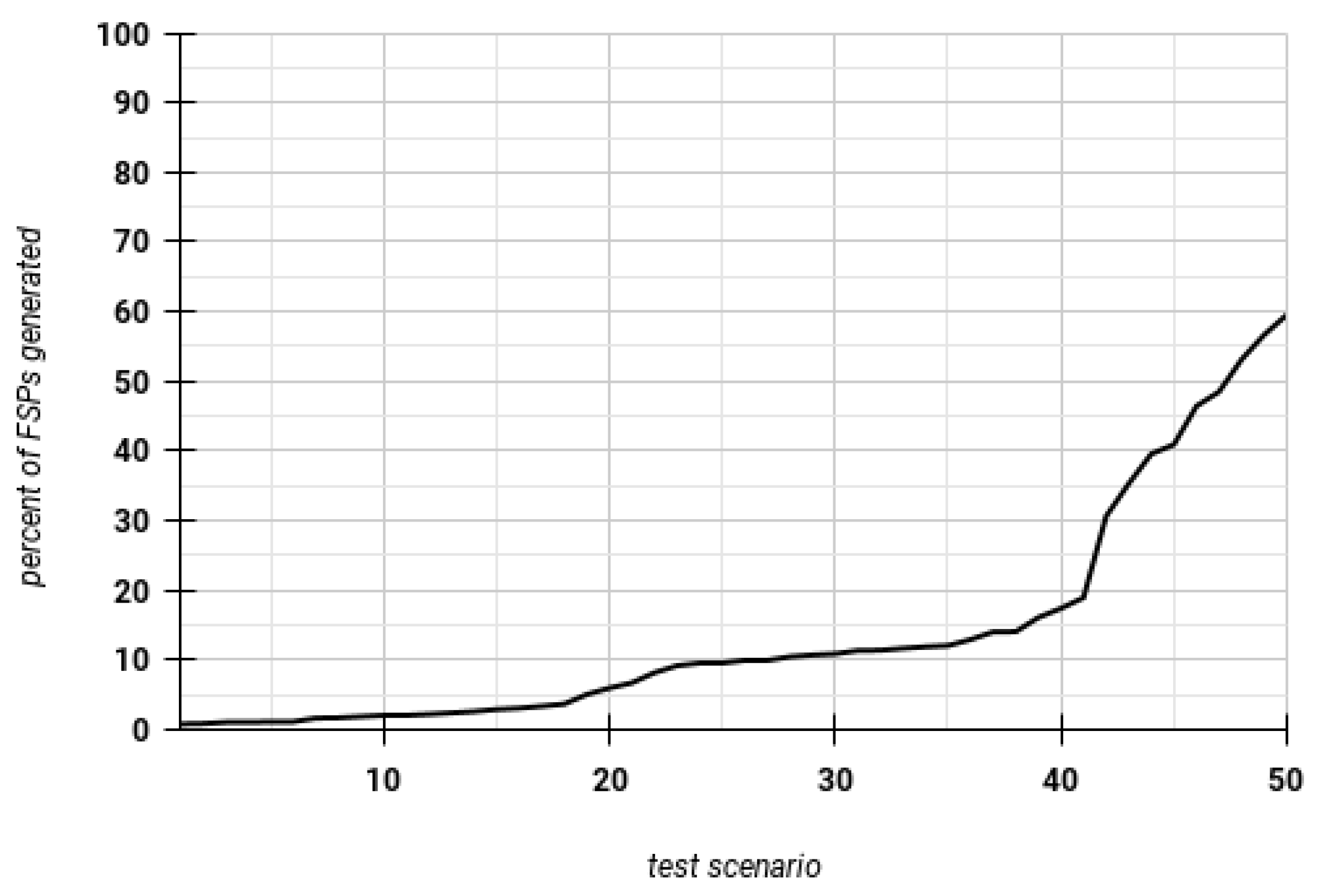
Figure 1. Percentages of FSPs generated by PSO-FSPMiner for each scenario in ascending order.
Algorithms 19 00229 g001
Figure 2. Overall accuracies of a KNN classifier that uses FSPs generated by PSO-FSPMiner for each scenario in descending order.
Algorithms 19 00229 g002
Table 1. Description of datasets.
DatasetsInstancesNon-Num.Num.Imbalance
Liver disorders3451627.5
Balance Scale576140.0
Pima indians diabetes76818116.0
Glass Identification146193.0
Indian Liver Patient57929124.5
Credit Approval6909738.0
Breast Cancer Wisconsin68319102.5
Diagnosis1207124.2
Cryotherapy90523.0
Algerian Forest Fires24421011.3
Table 2. Experimental results.
FSPsBehaviour
DatasetsFreqX-FSPMinerPSO-FSPMiner%O Acc
0.0216,434140 (22.38)0.85%81% (0.02)
0.049716165 (46.39)1.69%80% (0.02)
Liver Disorders0.066618145 (17.98)2.19%79% (0.02)
0.084800124 (13.14)2.58%78% (0.01)
0.103518108 (12.74)3.06%75% (0.02)
0.0253063 (12.41)11.88%80% (0.00)
0.0434255 (2.57)16.08%87% (0.00)
Balance Scale0.0623040 (1.42)17.39%90% (0.00)
0.089830 (0.75)30.61%83% (0.00)
0.106632 (0.00)48.48%81% (0.00)
0.02528100 (34.02)18.93%87% (0.01)
0.0418272 (16.89)39.56%88% (0.02)
Diabetes0.068439 (5.745)46.42%92% (0.02)
0.084225 (0.00)59.52%95% (0.00)
0.103017 (0.00)56.66%96% (0.00)
0.023062429 (23.65)14.01%96% (0.01)
0.0424234 (0.77)14.04%100% (0.00)
Glass0.066824 (0.45)35.29%100% (0.00)
0.083217 (0.47)53.12%100% (0.00)
0.10229 (0.15)40.90%100% (0.00)
0.02357,6483739 (285.92)1.04%85% (0.04)
0.04231,1662588 (216.83)1.11%82% (0.04)
Indian Liver Patient0.06165,6081298 (46.03)0.78%83% (0.03)
0.08120,2281270 (25.80)1.05%84% (0.03)
0.1095,7841288 (15.59)8.16%81% (0.04)
0.0270,7006749 (387.01)9.54%83% (0.02)
0.0423,3242644 (179.98)11.33%85% (0.02)
Credit Approval0.0612,9801414 (43.89)10.86%84% (0.01)
0.088378876 (28.69)10.45%84% (0.03)
0.106032703 (48.90)11.65%86% (0.03)
0.0210,756257 (5.40)2.38%93% (0.01)
0.044906142 (4.41)2.89%94% (0.01)
Breast0.063604132 (3.39)3.66%93% (0.01)
0.082524127 (2.01)5.03%93% (0.01)
0.101908128 (1.82)6.70%94% (0.02)
0.0211,9471142 (10.60)9.55%84% (0.03)
0.0410,3421107 (7.50)10.70%80% (0.04)
Diagnosis0.066383726 (7.45)11.37%77% (0.01)
0.084594421 (29.30)9.16%76% (0.04)
0.103454343 (4.86)9.93%77% (0.05)
0.028600288 (6.42)3.34%82% (0.01)
0.042588154 (5.92)5.95%84% (0.01)
Cryotherapy0.061178117 (2.22)9.93%84% (0.01)
0.0854866 (2.55)12.04%84% (0.01)
0.1035646 (2.31)12.92%85% (0.00)
0.02216,8982448 (5.38)1.12%85% (0.05)
0.0481,7381338 (9.55)1.63%88% (0.04)
Algerian0.0644,986918 (3.56)2.04%86% (0.03)
0.0829,246594 (2.56)2.03%89% (0.06)
0.1021,646404 (3.99)1.86%87% (0.05)
Table 3. Ranking of differences between the precision values obtained with respect to the different frequency thresholds tested.
0.040.060.080.1
0.020.850.100.750.20
0.04 0.750.100.65
0.06 0.650.10
0.08 0.55
Critical difference ( α = 0.05 ) = 1.92
Disclaimer/Publisher’s Note: The statements, opinions and data contained in all publications are solely those of the individual author(s) and contributor(s) and not of MDPI and/or the editor(s). MDPI and/or the editor(s) disclaim responsibility for any injury to people or property resulting from any ideas, methods, instructions or products referred to in the content.