Optimizing the Permutation Flowshop Scheduling Problem with an Improved Sparrow Search Algorithm

Abstract

The Sparrow Search Algorithm (SSA) is a novel optimization method inspired by sparrows’ foraging and anti-predator behavior. It mimics their exploration and exploitation strategies to find near-optimal solutions for various optimization problems. This paper presents the first application of SSA to the widely recognized Permutation Flowshop Scheduling Problem (PFSP) with the makespan criterion as the optimization target. Our study aims to assess the effectiveness and robustness of this cutting-edge metaheuristic through computational experiments and statistical analysis. The proposed SSA is a hybrid variant that incorporates the Variable Neighborhood Search (VNS) algorithm along with a Path Relinking Strategy. The effectiveness of the proposed method is evaluated through computational experiments on PFSP benchmark instances. The performance of the hybrid SSA is compared against several well-established swarm-intelligence metaheuristics, namely Grey Wolf Optimizer (GWO), Whale Optimization Algorithm (WOA), Tuna Swarm Optimization Algorithm (TSO), Particle Swarm Optimization Algorithm (PSO), Firefly Algorithm (FA), Bat Algorithm (BA), and the Artificial Bee Colony (ABC). To ensure fair comparison, all methods are implemented within the same computational framework as the hybrid SSA. The experimental results show that the proposed hybrid SSA achieves the lowest average mean error compared with the competing methods in solving the PFSP. The results were further validated through a comprehensive non-parametric statistical analysis using Friedman, Aligned Friedman, and Quade tests, followed by post-hoc analysis with p-adjusted values, as well as Kruskal–Wallis and Wilcoxon post-hoc tests.

1. Introduction

This study investigates the potential of a relatively new and effective, yet not widely adopted, swarm intelligence algorithm—the Sparrow Search Algorithm (SSA) [1]—in addressing the Permutation Flowshop Scheduling Problem (PFSP) [2]. Due to its inherent ability to balance exploration (global search) and exploitation (local search), the SSA shows great promise for solving combinatorial optimization problems, such as the PFSP. The SSA’s dynamic switching between these modes, inspired by the behavior of sparrows, makes it well-suited for improving schedules by reducing the total processing time or optimizing other performance objectives in PFSP. The SSA has been applied to a variety of optimization tasks, including feature selection [3], energy consumption [4], scheduling [5], engineering problems [6], communication problems [7], and several other applications, as indicated by the study of Awadallah et al. [8]. However, no documented studies have been found that specifically address its application to the PFSP. Therefore, the authors of this study seized the opportunity to investigate the potential of the SSA for solving this particular problem.

The PFSP is widely encountered in industries like automotive, electronics, and textiles, where the products must pass through multiple machines or stages in a specific sequence. The objective is to minimize the total processing time, commonly referred to as the makespan. Minimizing the makespan becomes increasingly important as the problem’s size grows. The PFSP is classified as an NP-hard problem [9], meaning that as the dimensions of the problem increase, the computational time required to find an optimal solution grows exponentially. Given these considerations, there is always a demand for effective methods to address the PFSP efficiently and promptly.

The proposed solution method incorporates a hybrid version of the SSA with Variable Neighborhood Search (VNS) [10] and two variations of the path-relinking strategy [11]. This combination further enhances the SSA’s potential for finding high-quality solutions.

It is widely accepted that the initial population of solutions, which is necessary for the function of most SI algorithms, plays a crucial role in determining the method’s overall efficiency. Employing heuristic algorithms to generate the initial population of solutions is a strategy that ensures the starting point leads to near-optimal solutions. The Nawaz, Enscore, and Ham (NEH) [12] algorithm provides an optimal solution for the two-machine PFSP, though its effectiveness decreases as the problem’s size increases. Nevertheless, the NEH algorithm can still be utilized to generate the initial population of solutions. Heuristics based on deterministic algorithms, such as NEH, will consistently generate the same solution for the same problem, as there is no randomness involved in their operations. To introduce a random element into the NEH process, we utilize a triangular distribution, allowing the randomized NEH to generate an initial population of distinct solutions.

Metaheuristic methods like the VNS, as well as the Path Relinking strategy, further improve the quality of the solutions as provided by the SSA. Both methods are explicitly discussed in Section 4.5. The proposed hybrid SSA employs the randomized NEH to generate the initial population of solutions. The generated solutions are then updated according to the basic formulations of SSA (Section 4.2). Thereafter, they are improved using the first version of Path Relinking, followed by the application of VNS. Next, the second version of Random Path Relinking is performed, and finally, the solutions are further refined through a second application of VNS.

For experimentation, seven prominent swarm intelligence (SI) metaheuristic algorithms were specifically developed and implemented using the same hybridization scheme as that employed in hybrid SSA. Specifically, the Grey Wolf Optimizer (GWO) [13], Tuna Swarm Optimization (TSO) [14], Whale Optimization Algorithm (WOA) [15], Firefly Algorithm (FA) [16], Particle Swarm Optimization (PSO) [17], Bat Algorithm (BA) [18], and Artificial Bee Colony (ABC) [19] are hybridized with the randomized NEH, VNS, and two version of Path Relinking, and were adapted accordingly to solve the PFSP. Their results were collected to compare their effectiveness against hybrid SSA. These algorithms have been shown to perform efficiently on a variety of combinatorial optimization problems and were therefore selected for comparative analysis. Overall, hybrid SSA achieves the lowest average mean error on the Taillard benchmark datasets [20], followed by hybrid versions of WOA, GWO, TSO, and FA, which constitute its strongest competitors.

To assess the alleged advantage of hybrid SSA over other algorithms, a statistical analysis was conducted using non-parametric tests, including Friedman, Friedman Aligned Ranks, and Quade, to identify any performance differences among the algorithms. Statistically significant results derived from these tests were collected, and further analysis was performed. Specifically, p-adjusted values were employed in these tests, thereby securing the validity of the results and enhancing their statistical significance. Furthermore, a complementary statistical analysis was performed using the Kruskal–Willis test by Wilcoxon pairwise and multiple comparisons and corrections. The results indicate that hybrid SSA differs statistically significantly from hybrid variants of PSO, BA, and ABC, whereas no statistically significant differences are detected with respect to hybrid variants of GWO, TSO, WOA, and FA. These results are consistent with the main non-parametric testing procedures, namely the Friedman, aligned Friedman and Quade tests. In contrast, the Kruskal–Willis omnibus test does not reveal differences in the error distributions across all algorithms. Statistical analysis based on box plots and descriptive statistical measures, such as mean, median, standard deviation, dispersion, as well as the minimum and maximum values across all benchmark sets, suggests that hybrid SSA maintains comparatively low variability across all sets. While it is not the lowest-variance method in every case, its variability remains consistently low relative to most competing algorithms (hybrid variants of GWO, TSO, WOA, and FA). This fact supports the claim that hybrid SSA performs in a stable manner.

This paper is organized as follows: In Section 2, an overview of the existing literature is presented. In Section 3, the definition of the permutation flowshop scheduling problem is explained, and Section 4 examines the main characteristics of the SSA, detailing each method presented, its purpose, and how it functions. In Section 5, a comparative study is conducted between hybrid SSA and other SI algorithms, along with a thorough statistical analysis to determine whether any algorithm demonstrates superior performance from a statistical perspective, and finally, in Section 6, conclusions and future research are given.

2. An Overview of Existing Literature

The SSA was developed by Xue J. and Shen B. in 2020 [1] and has since attracted the interest of researchers from various fields due to its fast convergence behavior and ease of implementation. Numerous studies have investigated its performance and proposed improvements or applications in different optimization domains, including the works of Li et al. [21], Song et al. [22], Ahmed et al. [23], Gai et al. [24], Zhang and Han [25], Xue et al. [26], Tao et al. [27], and Wu et al. [28].

Specifically, the SSA is employed in a variety of applications, as described in the Introduction, and has been modified for the purposes of different studies. Researchers improved SSA performance and searching capability by introducing hybrid variations, including chaotic strategy, adaptive strategy, binary mechanism, and multi-objective technique. In particular, the SSA has been combined with PSO [29,30], Water Wave Optimization (WWO) [31], Firefly Algorithm (FA) [32], Whale Optimization Algorithm (WOA) [33], and Grey Wolf Optimizer (GWO) [34]. Moreover, Yao et al. [35] studied the classical SSA, which was hybridized with the simulated annealing (SA) algorithm. Khaleel [36] showed that the SSA combined with Differential Evolution (DE) [37,38] achieves superior performance. According to the study of Gharehchopogh et al. [39], combining the SSA with other metaheuristics results in methods that enhance exploitation and convergence, strengthen the initial population, and improve global search, helping to avoid local optima. Moreover, numerous approaches have been developed in recent years to enhance SSA, including Chaos [40,41], Gaussian [42], Lévy flight [43], Opposition-Based Learning (OBL) [44], Random Walk [45], adaptive strategy [46] as well as Artificial Neural Networks (ANNs) [47] and Deep Learning [48].

Regarding scheduling, the literature contains a limited number of studies [5,47,49] investigating the potential of the SSA for this type of problem. In the context of optimization problems, scheduling refers to finding the most efficient way to allocate limited resources (like time, machines, workers, or space) to a set of tasks, often to minimize or maximize some objective. There are different categories of scheduling, such as job shop scheduling, flowshop scheduling [50], and many others, each of which includes various subtypes and variations. The SSA is utilized in two studies regarding the Flexible Job Shop Scheduling Problem (FJSP), according to the reviewed literature. In the first study, Wu et al. [5] solved the classic FJSP using the SSA and compared the results with those obtained from other metaheuristics, concluding that the SSA outperformed all others. Luan et al. [51] present an improved SSA that consists of the hybrid search (HS), quantum rotation gate (QRG), sine–cosine algorithm (SCA) [52], adaptive adjustment strategy (AAS), and VNS for tackling the Energy Saving FJSP. In ref. [49], a multi-strategy improved sparrow search algorithm (MISSA) was proposed for minimizing the makespan in the concept of Job Shop Scheduling (JSP). The classical SSA is extended by incorporating an operation-sequence encoding scheme for discrete scheduling, a tent chaotic mapping for population initialization, genetic crossover, and mutation operators to improve diversity and local search, and simulated annealing (SA) to avoid local optima.

The PFSP has garnered significant attention from researchers since the introduction of Johnson’s algorithm, the earliest known method for solving this problem [53]. Over the years, various approaches have been developed to address PFSP, including exact methods, heuristics, metaheuristics, hybrid metaheuristic methods—the most popular approach—and, more recently, machine learning techniques. A recent literature review on PFSP with makespan criterion is provided in ref. [2]. Recent research on PFSP from 2017 to 2025 shows a strong shift towards hybrid and improved solution approaches, especially for the makespan criterion and large benchmark instances. A hybrid Monkey Search algorithm (HMSA) in ref. [54] combines Monkey Search with NEH, SPT/LPT dispatching rules, SVP encoding, and mutation-based improvement, while the method in [55] enhances a gravitational emulation local search framework to improve exploration and exploitation. The hybrid Crow Search Algorithm in [56] incorporates NEH-based initialization, SVP encoding and a Simulated Annealing (SA)—VNS local search. Additionally, in [57] the adaptive PSO approach hybridizes the search process through simultaneous parameter adaptation and solution optimization. Similarly, the memetic algorithm in ref. [58] combines a genetic search, simulated annealing and a semi-constructive crossover and mutation operators guided by NEH-based principles. Moreover, in ref. [59], the hybrid Improved Efficient Genetic Algorithm integrates an elitism-based GA, uniform and arithmetic crossover, LRV-based mapping, local search, and insert-reversed block operator for optimizing the PFSP with the makespan criterion. In ref. [60], hybridization takes the form of a critical-path-based neighborhood search embedded within an improved simulated annealing framework, whereas the QABC method in ref. [61] combines the ABC algorithm with Q-learning-based adaptive neighborhood selection, multiple neighborhood structures, and insert-based improvement operators. Likewise, the improved simulated annealing in ref. [62] hybridizes solution-space clipping based on generalized Johnson’s rule and a Palmer release strategy. The hybrid GWO in ref. [63] combines a randomized NEH initialization, GWO, VNS and Path Relinking strategy. Even recently developed deterministic heuristics, such as the Variable Block Insertion Heuristic (VBIH) in ref. [64] and vN-NEH+ in ref. [65], rely on strong hybrid design through a combination of constructive initialization, block insertion or candidate list strategies, and partial or complete local improvement procedures. Alternative approaches such as exact branch-and-bound optimization [66] and deep reinforcement learning with NEH-based refinement [67] confirm that high-quality PFSP performance depends on effective interaction between initialization, encoding, and decoding techniques, local search and diversification mechanisms. However, most previous studies focus on a single algorithm under its own hybrid design. In contrast, the present study contributes not only by presenting the hybrid SSA but also by applying the same hybridization framework across multiple swarm-intelligence metaheuristics, which enables a fair and more controlled comparison of the underlying search mechanisms of the test methods.

3. Problem Description

The Permutation Flowshop Scheduling Problem

The Permutation Flowshop Scheduling Problem (PFSP) can be mathematically formulated as an optimization problem. Let’s denote the set of n jobs as $N=\{1, 2, \dots , n\}$ and a set of m machines as ${\rm M}=\{ 1, 2, \dots m\}$. The objective is to find a permutation $\pi =\{{\pi }_{1, }{ \pi }_{2 },\dots , {\pi }_n\}$ of the jobs for each machine that minimizes makespan ($C_{max}$). The basic assumptions for the PFSP are as follows:

• The sequence of jobs must be processed on the machines in the same order, i.e., from machine 1 to machine m.
• Each machine must process the jobs according to the given permutation.
• No preemption is allowed, meaning the processing of a job ${\pi }_i$ on the $j^{th}$ machine cannot be interrupted.
• All jobs are independent and available for processing at time zero.
• Each job is restricted to being processed on a single machine at any given time, and similarly, each machine can process only one job.
• Set-up times for jobs on machines are negligible and, therefore, can be disregarded.
• Furthermore, the machines are continuously available and waiting for the next operation.
• The transportation time for delivering one job between the machines is neglected.

According to a certain $\pi$ permutation of jobs, the job ${\pi }_i$ is placed at the $i^{th}$ position while $C_{{\pi }_{i}j}$ denotes the completion time of that job on the machine j. The variable $p_{{\pi }_{i}j}$ denotes the processing time for the job ${\pi }_i$ on the j machine. The mathematical description of the problem is provided in the following lines:

$$C_{{\pi }_1,1}= p_{{\pi }_{1,}1}$$

(1)

$$C_{{\pi }_i,1}=C_{{\pi }_{i-1},1}+p_{{\pi }_i,1}\hspace{1em}\forall i=2,\dots ,n$$

(2)

$$C_{{\pi }_{1,}j}=C_{{\pi }_1,j-1}+p_{{\pi }_1,j}\hspace{1em}\forall j=2,\dots ,m$$

(3)

$$C_{{\pi }_i,j}=\max \left\{C_{{\pi }_{i-1},j},C_{{\pi }_i,j-1}\right\}+p_{{\pi }_i,j} \hspace{1em}\forall i=2,\dots ,n;\forall j=2,\dots ,m.$$

(4)

The makespan of the permutation $\pi$ is defined as the completion time of the last job ${\pi }_n$ on the last machine m i.e.,

$$C_{\mathrm{m}\mathrm{a}\mathrm{x}}\left(\pi \right)=C({\pi }_n,m).$$

(5)

Therefore, the PFSP with the makespan criterion is to find the optimal permutation ${\pi }^{\ast }$ in the set of all possible permutations $\Pi$, such as:

$$C_{\mathrm{m}\mathrm{a}\mathrm{x}}\left({\pi }^{\ast }\right)\le C\left({\pi }_n,m\right)\hspace{1em}\forall \pi \in \Pi .$$

(6)

4. The Sparrow Search Algorithm (SSA): Methodology and Implementation

4.1. SSA Characteristics and Assumptions

Jiankai Xue and Bo Shen introduced the Sparrow Search Algorithm (SSA) [1], an optimization metaheuristic method inspired by the natural behavior of sparrows. More precisely, it mimics the behavior of sparrows by emulating their exploration and exploitation strategies. Similar to a sparrow foraging for food by searching various locations and exploiting fruitful ones, SSA explores the solution space by generating potential solutions and evaluating their effectiveness. This exploration process is akin to the random exploration of sparrows as they navigate their surroundings. Additionally, SSA incorporates exploitation strategies to refine and improve promising solutions, mirroring the way sparrows return to known food sources to gather more resources. This exploitation phase involves refining the solutions based on local information, similar to how sparrows leverage their knowledge of the environment to optimize their foraging efficiency. The mathematical model of the SSA is formulated based on the natural behavior of sparrows as they search for food or avoid predators, according to the following assumptions:

• Within the population of sparrows, two groups of individuals exist: the “producers” and the “scroungers”. The producers exhibit high energy reserves and act as leaders by identifying areas with rich food sources for the entire group, termed “scroungers.” The energy levels of the individuals depend on the assessment of the fitness values.
• If a sparrow detects a predator, it promptly emits an alarming signal, and if the alarm value surpasses the safety threshold, the producers guide all sparrows to a safe area.
• Each sparrow can switch between the producer and scrounger categories depending on its fitness value, while maintaining a consistent proportion of producers to scroungers within the population.
• Only the sparrows with high energy levels behave as producers. Several scroungers with depleted energy reserves are likely to search for food in different areas.
• Scroungers trail behind producers who offer the best food sources, aiming to augment their energy reserves. Some scroungers may compete for food resources, leading to an increase in their individual predation rates.
• In the face of imminent danger, the sparrows situated at the periphery of the group move toward the safe area, while the individuals in the center move randomly closer to the other members.

4.2. Mathematical Model

The position of the sparrows can be formulated as follows:

$$X= \left[\begin{array}{ccc}{x}_{\mathrm{1,1}}& \dots & x_{1,d}\\ ⋮& \ddots & ⋮\\ x_{n,1}& \dots & x_{n,d}\end{array}\right]$$

(7)

The $X$ represents the matrix with the positions of sparrows, where n is the number of sparrows and d is the dimension of the variables to be optimized.

The fitness value of all sparrows can be expressed by the following vector:

$$F_x=\left[\begin{array}{ccc}f\left(\right[x_{\mathrm{1,1}} x_{\mathrm{1,2}}& \dots & x_{1,d}\left]\right)\\ ⋮& \ddots & ⋮\\ f\left(\right[x_{n,1} x_{n,2}& \dots & x_{n,d}\left]\right)\end{array}\right]$$

(8)

where $F_x$ represents the fitness value of the individual.

The location of the producer is formulated as follows:

$$X_{i,j}^{t+1 }=\left\{\begin{array}{cc}{ X}_{i,j}^{t }·exp\left({\displaystyle \frac{-i}{a·ite{r}_{max}}}\right)\hfill & if R_2<ST\hfill \\ X_{i,j}^{t }+Q·L\hfill & if R_2\ge ST\hfill \end{array}\right.$$

(9)

where t is the current iteration, $j=1, 2,\dots d$ is the dimension of the problem, and $X_{i,j}^t$ represents the value of the jth dimension of the ith sparrow at iteration t. $ite{r}_{max}$ is a constant with the largest number of iterations. The $\alpha$ is a random number within the range of $\left(\mathrm{0,1}\right]$. The variables $R_2 \in \left[\mathrm{0,1}\right]$ and $ST \in [0.5,1]$ are the alarm and the safety threshold, respectively. Q is a random number in [0, 1] and L is a matrix $1 \times d$ with ones.

• If $R_2<ST$: in this case, there is no imminent danger for the sparrows, and the producer searches a wider area for resources.
• If $R_2\ge ST$: the same sparrows have detected a predator, and they all fly to a safety area.

The scroungers update their location according to Equation (10). The scroungers monitor the producers, and upon discovering that the producers have located a food source, the scroungers abandon their current position and engage in competition for the food. The mathematical formulation representing this behavior is as follows:

$$X_{i,j}^{t+1 }=\left\{\begin{array}{c}\begin{array}{cc}Q·exp\left({\displaystyle \frac{X_{worst }^t-X_{i,j}^t }{a·ite{r}_{max}}}\right) & if i>n/2\end{array}\\ \begin{array}{cc}{ X}_P^{t+1 }+\left|X_{i,j}^t- X_P^{t+1 }\right|·A^{+}·L& otherwise\end{array}\end{array}\right.$$

(10)

where $X_P$ is the optimal position of the producer and $X_{worst}$ denotes the global worst location according to the fitness value. A is a matrix with dimensions $1\times d$, and each element in that matrix is randomly filled with a value of 1 or −1. The $A^{+}$ matrix has the same dimensions as A and can be calculated as $A^{+}=A^T{\left(A{A}^T\right)}^{-1}$. $A^T$ represents the transpose of matrix A, and ${\left(A{A}^T\right)}^{-1}$ represents the inverse of the product of matrix A and its transpose. When $i>n/2$, the ith scrounger with the worst fitness value is more likely to starve.

The sparrows that perceive danger, called scouters, account for the 10% to 20% of the total population, and they act accordingly to assumption 6. The mathematical formulation that represents this behavior can be formulated as follows:

$$X_{i,j}^{t+1 }= \left\{\begin{array}{c}\begin{array}{cc}{X}_{best}^t+\beta ·\left|X_{i,j}^t- X_{best}^{t }\right| & if f_i>f_g\end{array}\\ \begin{array}{cc}{X}_{i,j}^{t }+K·\left({\displaystyle \frac{\left|X_{i,j}^t- X_{worst}^{t }\right|}{\left(f_i-f_w\right)+\epsilon }}\right)& if f_i=f_g \end{array}\end{array}\right\}$$

(11)

where $X_{best}$ is the current global best value (location) and β as the step size control parameter, is a normal distribution of random numbers with a mean value of 0 and a variance of 1. $K\in [-1,1]$ is a random number. $f_i$ is the fitness value of the ith sparrow. $f_g$ and $f_w$ are the current global best and the worst fitness values, respectively. ε is a small number to avoid division by zero.

4.3. Parameter Tuning

All the values of the parameters are listed below.

The number of producers is denoted as PD, and the number of sparrows who perceive danger is denoted as SD.

$$\begin{gathered} n=100 \\ ite{r}_{max}=20 \\ PD=75 \\ SD=25 \\ {R}_2=0.2 \\ \mathrm{ST}=0.6 \end{gathered}$$

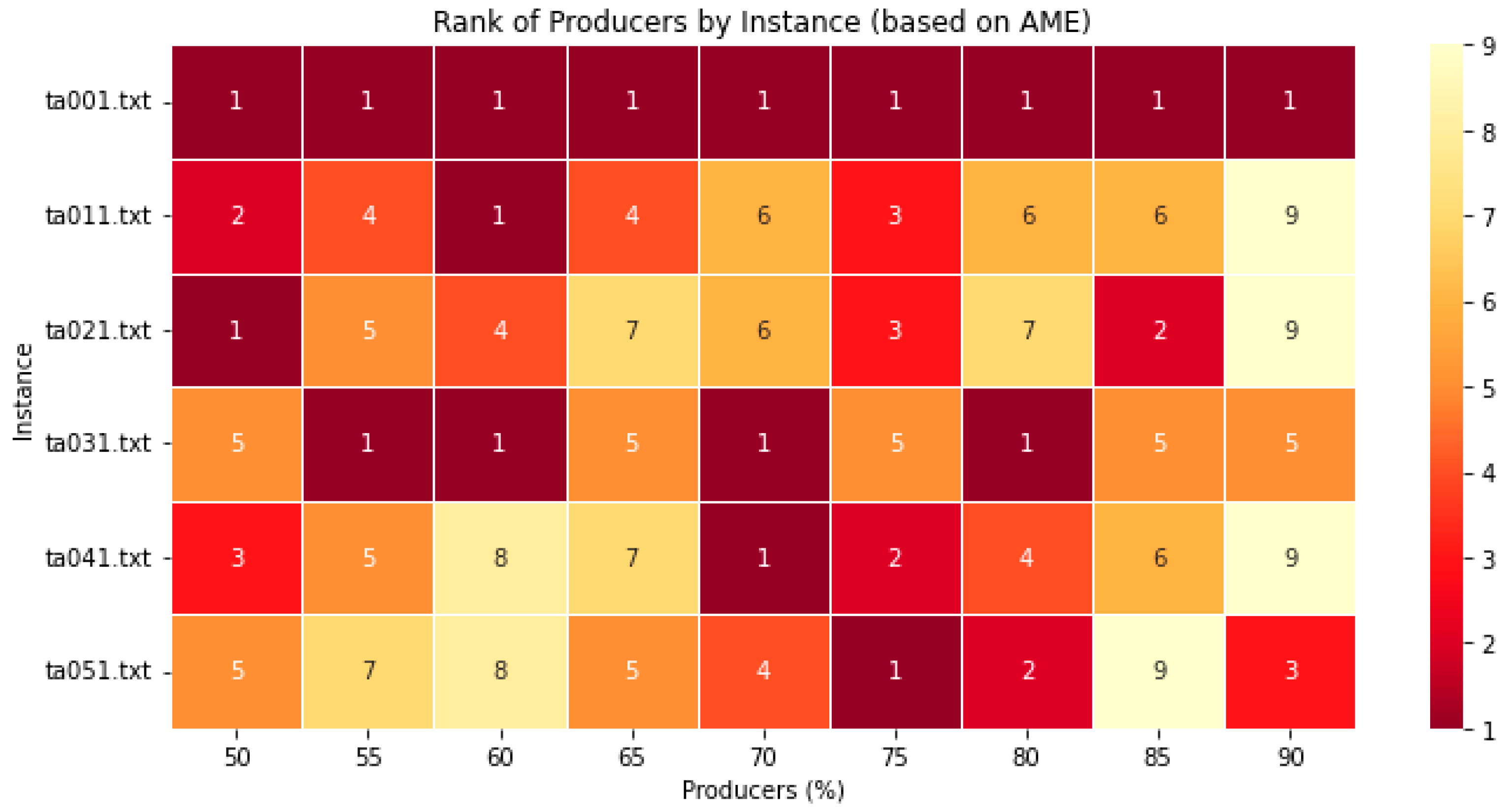
To conduct this experiment, we initially set the number of both producers and scroungers to 50 each. The objective was to determine the optimal ratio of producers and scroungers within the population. After conducting five rounds of testing, the maximum and minimum fitness values were recorded, and the average mean error was calculated. Subsequently, the number of producers was incrementally increased to 55 while the number of scroungers was decreased to 45. This process was repeated iteratively until the number of producers reached 90 and the number of scroungers diminished to 10. This process was applied to five different instances of each instance set (six in total), in order to ensure representation of different difficulty levels. Figure 1 shows the rankings by instance (Ta001, Ta021, Ta031, Ta041, and Ta051) based on average mean error (AME)—the experimental data are presented in detail in Section 5.1.

Table A1. Sensitivity analysis of the producer population size over five runs across five representative instances for each producer–scrounger population ratio.

Instance	Producers	Scroungers	Mean	Min	Max	Std	AME
Ta001	50	50	1283.4	1278	1297	8.35	0.00
Ta001	55	45	1279.6	1278	1286	3.58	0.00
Ta001	60	40	1279.6	1278	1286	3.58	0.00
Ta001	65	35	1283.4	1278	1297	8.35	0.00
Ta001	70	30	1281.2	1278	1286	4.38	0.00
Ta001	75	25	1279.6	1278	1286	3.58	0.00
Ta001	80	20	1282.2	1278	1286	3.77	0.00
Ta001	85	15	1283.4	1278	1297	8.35	0.00
Ta001	90	10	1279.8	1278	1286	3.49	0.00
Ta011	50	50	1597	1583	1614	11.40	0.06
Ta011	55	45	1597.4	1586	1613	10.06	0.25
Ta011	60	40	1590.4	1582	1605	9.07	0.00
Ta011	65	35	1605.6	1586	1614	11.41	0.25
Ta011	70	30	1600.6	1593	1607	5.32	0.70
Ta011	75	25	1599.6	1585	1607	7.06	0.19
Ta011	80	20	1605.4	1593	1618	10.50	0.70
Ta011	85	15	1596.4	1593	1601	3.44	0.70
Ta011	90	10	1605.4	1598	1618	7.99	1.01
Ta021	50	50	2325	2300	2341	17.33	0.13
Ta021	55	45	2324.8	2307	2332	10.11	0.44
Ta021	60	40	2327	2305	2348	15.22	0.35
Ta021	65	35	2323.4	2316	2333	7.70	0.83
Ta021	70	30	2327	2314	2338	9.11	0.74
Ta021	75	25	2327.2	2303	2339	9.23	0.26
Ta021	80	20	2323.2	2316	2329	5.89	0.83
Ta021	85	15	2319.2	2302	2335	15.06	0.22
Ta021	90	10	2338	2323	2354	11.25	1.13
Ta031	50	50	2729	2729	2729	0.00	0.18
Ta031	55	45	2728	2724	2729	2.24	0.00
Ta031	60	40	2728	2724	2729	2.24	0.00
Ta031	65	35	2729	2729	2729	0.00	0.18
Ta031	70	30	2728	2724	2729	2.24	0.00
Ta031	75	25	2729	2729	2729	0.00	0.18
Ta031	80	20	2728	2724	2729	2.24	0.00
Ta031	85	15	2729	2729	2729	0.00	0.18
Ta031	90	10	2729.4	2729	2731	0.89	0.18
Ta041	50	50	3090.6	3051	3126	32.42	2.01
Ta041	55	45	3075.4	3054	3087	12.54	2.11
Ta041	60	40	3084.6	3069	3108	15.52	2.61
Ta041	65	35	3079.8	3056	3126	28.32	2.17
Ta041	70	30	3068.6	3049	3105	22.86	1.94
Ta041	75	25	3080.4	3050	3113	24.03	1.97
Ta041	80	20	3073.6	3052	3126	29.90	2.04
Ta041	85	15	3087	3055	3106	20.26	2.14
Ta041	90	10	3102.2	3086	3126	18.14	3.18
Ta051	50	50	3987	3969	4009	17.09	3.09
Ta051	55	45	3986.4	3970	3995	10.43	3.12
Ta051	60	40	3997.6	3973	4016	16.12	3.19
Ta051	65	35	4009.6	3969	4031	26.06	3.09
Ta051	70	30	3989.2	3965	4014	18.21	2.99
Ta051	75	25	3996.2	3951	4027	20.97	2.62
Ta051	80	20	3972.2	3954	4001	20.00	2.70
Ta051	85	15	3990.4	3983	3999	6.47	3.45

records the mean fitness value as well as the maximum and minimum values across five independent runs for each producer-scrounger ratio and for six instances. The ranks were calculated separately for each instance based on the AME values, where the lowest AME received rank 1, and ties were assigned to the same minimum rank. The overall performance of each producer–scrounger ratio was then assessed using its average rank across all tested instances. Based on these values, Figure 1 portrays the rank of producer-scrounger ratios based on the average mean error derived from Table A1. Based on this analysis, we selected the 75% producers—25% scroungers ratio, as it is the only ratio that provides low ranks in the larger instances (Ta041 = 2 and Ta051 = 1) and generally good performance across all other testing instances.

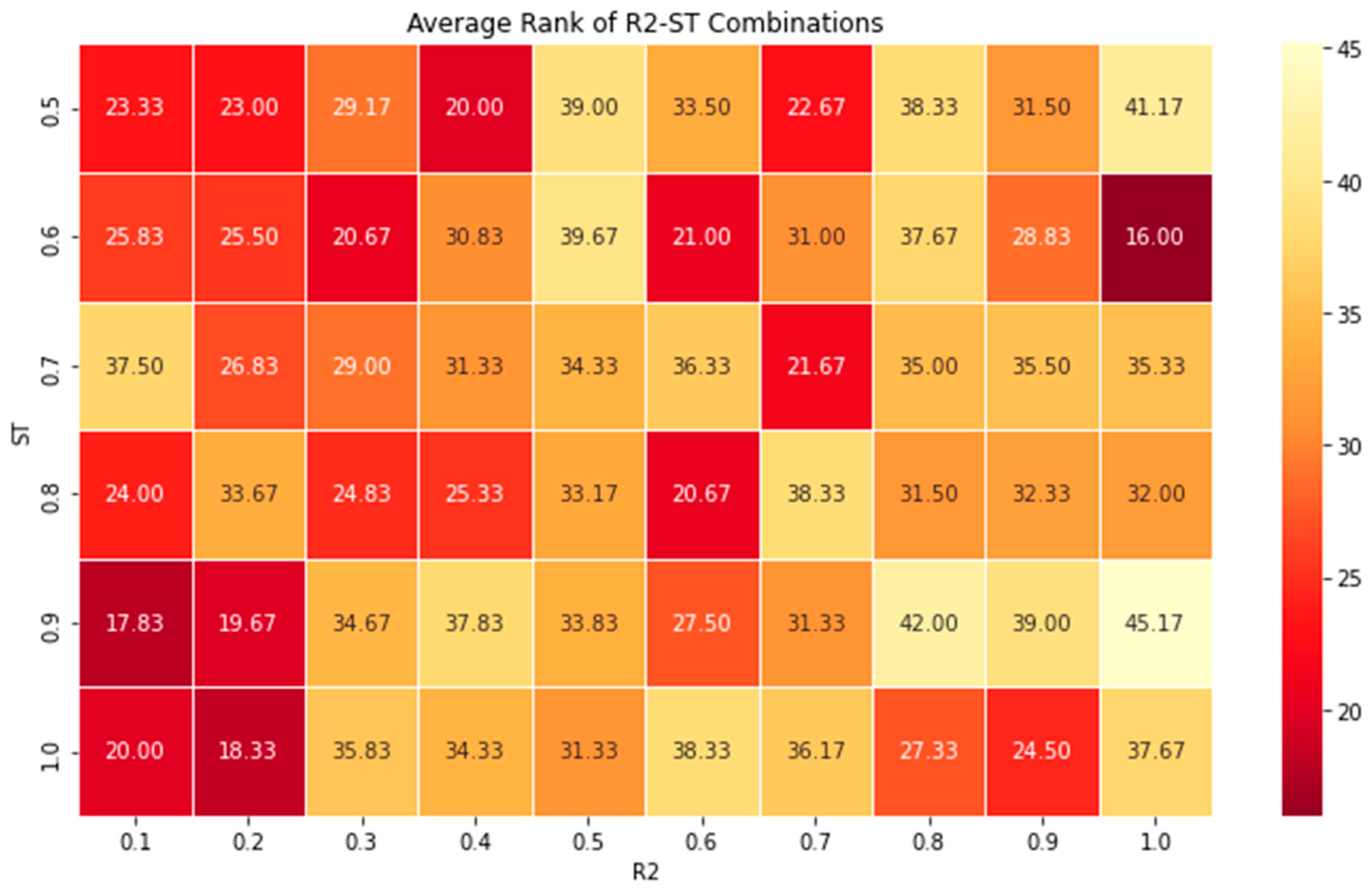
The selection of the ST threshold and the alarm value $R_2$ is guided by a sensitivity analysis, the results of which are depicted in Figure 2. After establishing the population of producers and scroungers, we conduct tests for each value of the ST parameter within the range of 0.5 to 1.0 along with each value of the alarm parameter $R_2$ within the range of 0.1 to 1.0. Following five rounds of each test, we record fitness values and calculate the average mean error for all six instances, namely ta001, ta011, ta021, ta031, ta041, and ta051. Since these instances belong to different difficulty levels, direct comparison based on raw objective values is not appropriate. For this reason, a rank-based analysis was adopted using the mean error as the primary performance criterion. The results reveal several optimal combinations for the ST and $R_2$ parameters of the hybrid SSA, pertaining to the permutation flowshop scheduling problem. Since the combination ST = 0.6 and R₂ = 0.2 lies within the low-average-rank region, its selection is justified. In general, parameter selection is highly sensitive to the characteristics of the data; therefore, the scope of the present analysis remains limited, since the testing was conducted using six representative instances, namely Ta001, Ta011, Ta021, Ta031, Ta041, and Ta051. The selected parameter values should therefore be regarded as robust within the scope of the tested Taillard instances, rather than as universally optimal settings for substantially larger benchmark problems.

4.4. Initial Solutions: The Proposed Nawaz, Encore, Ham (NEH) Algorithm

The Sparrow Search Algorithm (SSA) relies on an initial population, which can be generated randomly or using another randomized heuristic method. The significance of this initial population on the algorithm’s performance is widely recognized. Constructive heuristics play a crucial role in kickstarting exploration, whereas inadequate initial solutions may lead to premature convergence. In this study, we introduce a modified version of the NEH algorithm, a popular choice for initializing the Permutation Flowshop Scheduling Problem (PFSP). Our randomized NEH variant introduces a triangular distribution, injecting randomness into the insertion phase. By parameterizing the distribution with minimum (a), maximum (b), and mode (c) values, we ensure diversity in generated solutions.

We set those parameters according to the following formulations:

$$a=\min \left\{\sum _{\mathrm{j}=1}^{\mathrm{m}}{p}_{{\pi }_{1}j},\sum _{\mathrm{j}=1}^{\mathrm{m}}{p}_{{\pi }_{2}j},\dots ,\sum _{\mathrm{j}=1}^{\mathrm{m}}{p}_{{\pi }_{n}j}\right\}-{\displaystyle \frac{c}{2}}$$

(12)

$$\mathrm{b}=\max \left\{\sum _{\mathrm{j}=1}^{\mathrm{m}}{p}_{{\pi }_{1}j},\sum _{\mathrm{j}=1}^{\mathrm{m}}{p}_{{\pi }_{2}j},\dots ,\sum _{\mathrm{j}=1}^{\mathrm{m}}{p}_{{\pi }_{n}j}\right\}+c$$

(13)

$$c={\displaystyle \frac{\alpha +b}{2}}$$

(14)

where $\alpha \le c\le b$.

Instead of using classical NEH rule when constructing a permutation $\pi$, the proposed randomized NEH inserts each new job into the permutation according to the probability delivered from a triangular distribution. The parameters $a$ and $b$ correspond to the shortest and longest processing times, respectively. Owing to the triangular shape of the distribution, jobs with processing times close to the average are selected more frequently than the extremes cases, while still allowing to the latter to be chosen. Consequently, the randomized NEH can generate a variety of quality initial solutions. In this study, an initial population of n sparrows is established, with 70% produced by the randomized NEH and the remaining 30% generated randomly.

Encoding and Decoding Technique

When adapting the SSA algorithm for the PFSP, it’s imperative to reconcile the continuous nature of the algorithm’s solutions with the discrete nature of the job numbering. In order to achieve that, we employ a technique to transform the continuous solution space of the SSA into a permutation of jobs. Specifically, we map the smallest value of the SSA solution to the first job and proceed sequentially, assigning each subsequent value to the corresponding job. This process ensures that the largest value of the SSA solution corresponds to the total number of jobs, thereby creating a valid permutation for the PFSP.

To transform solutions from discrete to continuous form, we apply a technique where all elements are divided by the largest value in the solution. As a result, the elements in the sparrow range between 0 and 1, enabling utilization by the SSA algorithm.

4.5. SSA with Variable Neighborhood Search (VNS) and Path Relinking

4.5.1. The Proposed VNS Algorithm

The proposed Variable Neighborhood Search (VNS) procedure employs a local search mechanism to improve a provided solution s. Starting from the current solution s, one neighborhood structure k ∈ {1, 2, 3, 4, 5, 6} is randomly selected at each iteration from a set of six operators, namely, 2–opt, 3–opt, 1–0 relocate, 2–0 relocate, 1–1 exchange, and 2–2 exchange. Then, the selected operator is applied to the current solution $X_i$ to generate a new candidate solution $X^{\prime }$. The candidate solution $X^{\prime }$ is evaluated according to the objective function $f$($X^{\prime })$ and if there is an improvement, it is accepted as the current best solution ($X_{best}$) and the counter t is set to zero. Otherwise, the current solution $X_i$, remains unchanged and the counter t is increased by one. The search terminates when 20 consecutive neighborhood explorations fail to produce an improvement. In this way, the proposed VNS procedure intensifies the search around promising regions of the solution space while avoiding unnecessary evaluations when no further local improvement can be obtained. Within the framework of the SSA, the global search is determined by the mechanisms of producers and scroungers (Equations (10) and (11)) whereas, at the local level, the proposed VNS improves the obtained solutions through neighborhood-based moves. Therefore, the producers–scroungers mechanism and VNS operate in complementary manner, with SSA providing the candidate structures to be explored and VNS intensifying the search around these structures. The combination of diversification and intensification results in a more effective and balanced computational framework, thereby mitigating premature convergence through the interaction of complementary mechanisms. A detailed pseudocode of the proposed VNS is presented in Algorithm 1.

Algorithm 1. Variable Neighborhood Search (VNS)

Input: ${\mathrm{X}}_{\mathrm{i}}$: current solution $\mathrm{f}\left({\mathrm{X}}_{\mathrm{i}}\right)$: objective value of the solution ${\mathrm{X}}_{\mathrm{i}}$ Output: ${\mathrm{X}}_{\mathrm{b}\mathrm{e}\mathrm{s}\mathrm{t}}$: improved solution $\mathrm{f}\left({\mathrm{X}}_{\mathrm{b}\mathrm{e}\mathrm{s}\mathrm{t}}\right)$: objective value of the improved solution 1. Set the non-improvement counter t ← 0 2.   Set ${\mathrm{X}}_{\mathrm{b}\mathrm{e}\mathrm{s}\mathrm{t}}$ ← ${\mathrm{X}}_{\mathrm{i}}$ 3.   While t < 20 do 4.          Randomly choose a neighborhood structure k ∈ {1, 2, 3, 4, 5, 6} 5.          Generate a candidate solution ${\mathrm{X}}^{\prime }$ by applying the selected operator:                     k = 1: 2–opt                     k = 2: 3–opt                     k = 3: 1–0 relocate                     k = 4: 2–0 relocate                     k = 5: 1–1 exchange                     k = 6: 2–2 exchange 6.          Evaluate the objective value of the candidate solution $\mathrm{f}(\mathrm{X}$′) 7.          if $\mathrm{f}$(${\mathrm{X}}^{\prime }$) < $\mathrm{f}$(${\mathrm{X}}_{\mathrm{b}\mathrm{e}\mathrm{s}\mathrm{t}}$) then                     ${\mathrm{X}}_{\mathrm{b}\mathrm{e}\mathrm{s}\mathrm{t}}$ ← ${\mathrm{X}}^{\prime }$                     $\mathrm{f}$(${\mathrm{X}}_{\mathrm{b}\mathrm{e}\mathrm{s}\mathrm{t}}$) ←$\mathrm{f}$(${\mathrm{X}}^{\prime }$)                     t ← 0 8.              else                     t ← t + 1               end if 9.    End While 10.    Return best

4.5.2. The Proposed Path Relinking Strategy

In the context of this study, a path relinking method is applied where the starting solution is a sparrow in the population while the target solution is the best-known sparrow ($X_{best}$). In each iteration, another sparrow is selected as the starting point until all sparrows in the population are explored. This method involves systematically exploring paths between sparrows in the swarm, aiming to improve the overall quality of solutions. Following the path relinking, the VNS is employed for the solutions that have been improved previously. Then, an additional Path Relinking is performed 10 times between randomly selected pairs of solutions, introducing further interaction among candidate solutions. A second VNS phase is subsequently applied to all sparrows so as to refine the new solutions after the pairwise relinking. A pseudocode of the proposed path relinking is presented in Algorithm 2.

Algorithm 2. First version of path relinking

Input: ${\mathrm{X}}_{\mathrm{b}\mathrm{e}\mathrm{s}\mathrm{t}}$: global best solution ${\mathrm{X}}_{\mathrm{i}}$   : current sparrow solution $\mathrm{f}\left({\mathrm{X}}_{\mathrm{i}}\right)$: objective value of $\mathrm{X}$ calculated with Equation (6) Output: ${\mathrm{X}}_{{\mathrm{i}}_{\mathrm{b}\mathrm{e}\mathrm{s}\mathrm{t}}}$: improved solution $\mathrm{f}\left({\mathrm{X}}_{{\mathrm{i}}_{\mathrm{b}\mathrm{e}\mathrm{s}\mathrm{t}}}\right)$: objective value of the improved solution 1.   Set ${\mathrm{X}}_{{\mathrm{i}}_{\mathrm{c}\mathrm{u}\mathrm{r}\mathrm{r}\mathrm{e}\mathrm{n}\mathrm{t}}}$ ← ${\mathrm{X}}_{\mathrm{i}}$ 2.   Set ${\mathrm{X}}_{{\mathrm{i}}_{\mathrm{b}\mathrm{e}\mathrm{s}\mathrm{t}}}$ ← ${\mathrm{X}}_{\mathrm{i}}$ 3.   Set $\mathrm{f}\left({\mathrm{X}}_{{\mathrm{i}}_{\mathrm{b}\mathrm{e}\mathrm{s}\mathrm{t}}}\right)$ ← $\mathrm{f}\left({\mathrm{X}}_{\mathrm{i}}\right)$ 4.   Identify the positions at which ${\mathrm{X}}_{{\mathrm{i}}_{\mathrm{c}\mathrm{u}\mathrm{r}\mathrm{r}\mathrm{e}\mathrm{n}\mathrm{t}}}$ differs from ${\mathrm{X}}_{\mathrm{b}\mathrm{e}\mathrm{s}\mathrm{t}}$ 5.   While ${\mathrm{X}}_{{\mathrm{i}}_{\mathrm{c}\mathrm{u}\mathrm{r}\mathrm{r}\mathrm{e}\mathrm{n}\mathrm{t}}}$ is not identical to ${\mathrm{X}}_{\mathrm{b}\mathrm{e}\mathrm{s}\mathrm{t}}$  do 6.          Modify ${\mathrm{X}}_{{\mathrm{i}}_{\mathrm{c}\mathrm{u}\mathrm{r}\mathrm{r}\mathrm{e}\mathrm{n}\mathrm{t}}}$ with 1-1 exchange move so that it becomes closer to ${\mathrm{X}}_{\mathrm{b}\mathrm{e}\mathrm{s}\mathrm{t}}$ 7.          For each admissible move do                     Apply the move temporarily                     Evaluate the resulting intermediate solution               End For 8.           Select the intermediate solution with the best objective value 9.           Set ${\mathrm{X}}_{{\mathrm{i}}_{\mathrm{c}\mathrm{u}\mathrm{r}\mathrm{r}\mathrm{e}\mathrm{n}\mathrm{t}}}$ ← selected intermediate solution 10.         If ${\mathrm{f}(\mathrm{X}}_{{\mathrm{i}}_{\mathrm{c}\mathrm{u}\mathrm{r}\mathrm{r}\mathrm{e}\mathrm{n}\mathrm{t}}})$ < $\mathrm{f}\left({\mathrm{X}}_{{\mathrm{i}}_{\mathrm{b}\mathrm{e}\mathrm{s}\mathrm{t}}}\right)$ then ${\mathrm{X}}_{{\mathrm{i}}_{\mathrm{b}\mathrm{e}\mathrm{s}\mathrm{t}}}$← ${\mathrm{X}}_{{\mathrm{i}}_{\mathrm{c}\mathrm{u}\mathrm{r}\mathrm{r}\mathrm{e}\mathrm{n}\mathrm{t}}}$ $\mathrm{f}\left({\mathrm{X}}_{{\mathrm{i}}_{\mathrm{b}\mathrm{e}\mathrm{s}\mathrm{t}}}\right)$ ← ${\mathrm{f}(\mathrm{X}}_{{\mathrm{i}}_{\mathrm{c}\mathrm{u}\mathrm{r}\mathrm{r}\mathrm{e}\mathrm{n}\mathrm{t}}})$ 11.             End If 12.   End While 13.   Return ${\mathrm{X}}_{{\mathrm{i}}_{\mathrm{b}\mathrm{e}\mathrm{s}\mathrm{t}}}$, $\mathrm{f}\left({\mathrm{X}}_{{\mathrm{i}}_{\mathrm{b}\mathrm{e}\mathrm{s}\mathrm{t}}}\right)$

The only modification in the second method is the selection of target solution and starting solution, which happens randomly.

4.5.3. The Proposed Hybrid SSA Method

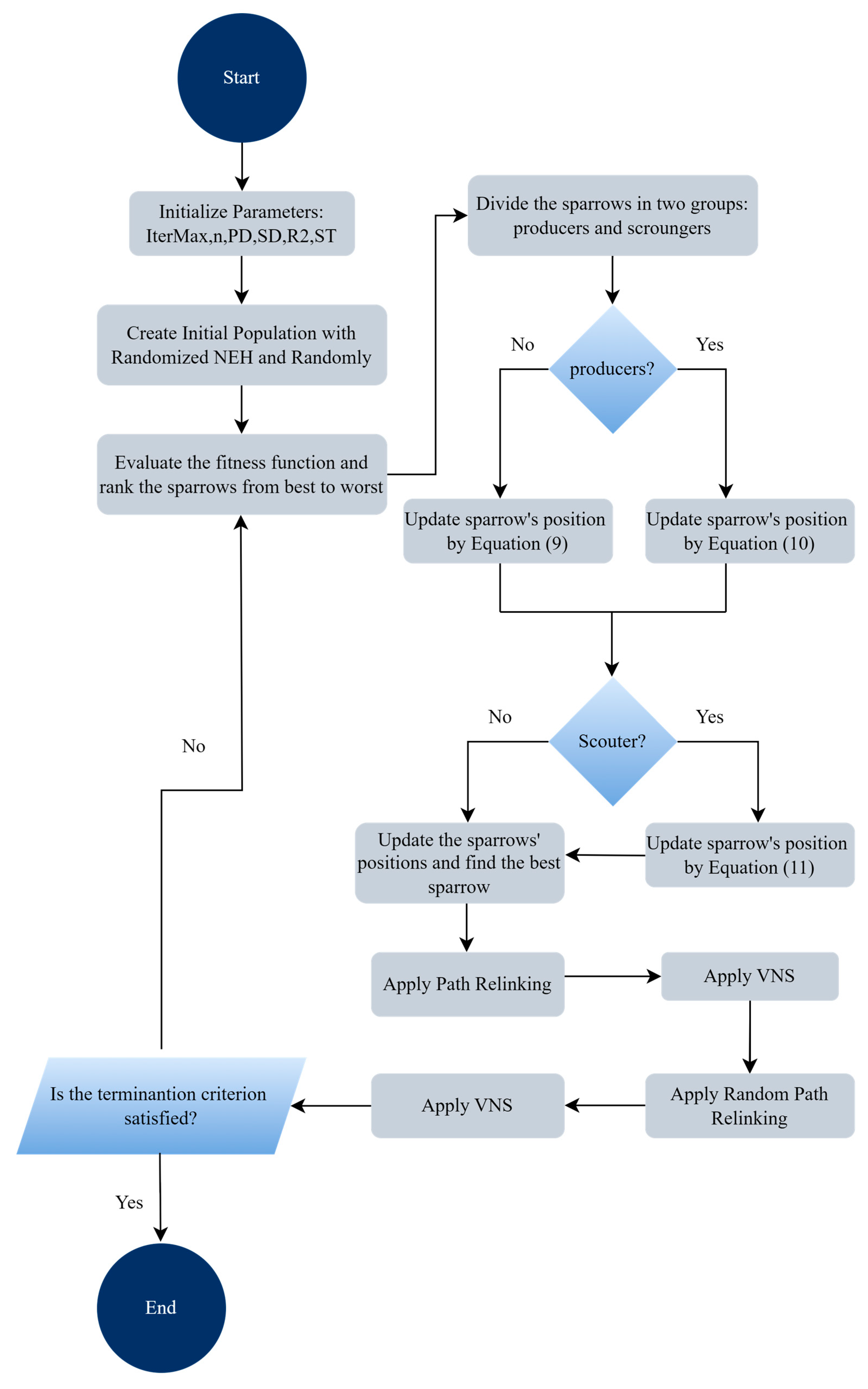
The flowchart of the proposed solution method is given as in Figure 3.

The proposed method (Figure 3) preserves the main population update mechanism of the standard SSA, provided by the Equations (9)–(11), while introducing a mixed initialization method, permutation conversion, Path Relinking and Variable Neighborhood Search as described previously. The combination of Path Relinking and VNS in the proposed hybrid SSA function is complementary, as Path Relinking enhances diversification in a guided manner, whereas VNS intensify the search for improved solutions through a systematic local mechanism. The complete pseudocode of the proposed hybrid SSA is presented in Algorithm 3.

Algorithm 3. Proposed hybrid SSA for the PFSP

1.   Import PFSP data from filename               Read n_jobs, m_machines and processing-time matrix data 2.   Set algorithm parameters 3.   Generate the initial population               For i = 1 to N − 50                      Sparrows[i] ← random permutation               End For               For i = N − 49 to N                      Sparrows[i] ← randomized NEH solution               End For 4.   Evaluate all sparrows using makespan (Equation (6)) 5.   Sort the population in ascending order of makespan 6.   For Iter = 1 to Max_Iter do 7.          Identify $X_{Best}$ ← best sparrow $X_{Worst}$ ← worst sparrow 8.          Producer phase              For i = 1 to P                     NewSparrows[i] ← producer update rule (Equation (9))              End For 9.          Evaluate updated producers              Determine $X_P$ = best producer 10.        Scrounger phase              For i = P + 1 to N                      NewSparrows[i] ← scrounger update rule using $X_{Worst}$ and $X_P$ (Equation (10))              End For 11.        Greedy replacement              For i = 1 to N                      Evaluate NewSparrows[i]                      If NewSparrows[i] improves Sparrows[i] then                            Replace Sparrows[i]                      End If              End For 12.        Sort the population 13.        Danger-alarm phase              Randomly select SD sparrows              For each selected sparrow k                     Generate a new solution using the danger-alarm rule (Equation (11))                     If the new permutation improves the current one then                           Replace it                     End If                End For 14.          Sort the population 15.          For each sparrow i = 1 to N                       Apply Path Relinking between $X_{Best}$ and Sparrows[i]                End For 16.           For each sparrow i = 1 to N                        Apply VNS local search to Sparrows[i]                End For 17.          Repeat 10 times                       Randomly select two sparrows                       Apply Path Relinking between them                End Repeat 18.           For each sparrow i = 1 to N                        Apply VNS local search again                End For 19.           Sort the population 20. End For 21. Return the best makespan found

5. Computational Experiments and SSA Evaluation Against Other Swarm Intelligence Metaheuristics

5.1. SSA Computational Experiments on Benchmark Datasets

This section presents the results for the makespan criterion obtained from the Hybrid Sparrow Search Algorithm—hybrid SSA. To facilitate comparative analysis, benchmark datasets from Taillard’s work [20] are utilized to evaluate the proposed solution algorithms. Two sets of problems are considered: one with 20 jobs and the other with 50 jobs. Each set encompasses varying numbers of machines, including 5, 10, and 20. Within each combination of jobs and machines, there are 10 distinct problem instances. In total, there are six problem sets: 20 × 5 (20 jobs and 5 machines), 20 × 10, 20 × 20, 50 × 5, 50 × 10, and 50 × 20. For each problem instance, we conducted 10 rounds of experimentation, recording both the average and the best obtained values.

Table 1. Results of the hybrid SSA for the PFSP with makespan criterion using Taillard’s benchmark datasets (AME is given in bold formatting in order to emphasize its importance).

Instance	BKS	${\mathit{C}}_{\mathit{S}\mathit{S}\mathit{A}}$	AVG	St. Dev.	ME (%)	Instance	BKS	${\mathit{C}}_{\mathit{S}\mathit{S}\mathit{A}}$	AVG	St. Dev.	ME (%)
Ta001	1278	1278	1278	0.00	0.00	Ta031	2724	2724	2728	2.11	0.00
Ta002	1359	1359	1363.2	1.10	0.00	Ta032	2834	2838	2846.7	6.25	0.14
Ta003	1081	1081	1088.1	0.33	0.00	Ta032	2621	2621	2626.6	3.60	0.00
Ta004	1293	1293	1293	0.00	0.00	Ta033	2751	2762	2774.2	9.34	0.40
Ta005	1235	1235	1226.2	1.04	0.00	Ta034	2863	2864	2864	0.00	0.03
Ta006	1195	1195	1195	0.00	0.00	Ta035	2829	2831	2832.8	1.62	0.07
Ta007	1239	1239	1243.5	2.31	0.00	Ta036	2725	2728	2732.7	2.41	0.11
Ta008	1206	1206	1210.1	1.97	0.00	Ta037	2683	2683	2686.5	7.55	0.00
Ta009	1230	1230	1235.2	3.14	0.00	Ta039	2552	2555	2560.1	3.18	0.12
Ta010	1108	1108	1111.3	2.03	0.00	Ta040	2782	2782	2782.3	0.48	0.00
AME				1.19	0.00					3.65	0.09
Ta011	1582	1582	1596.2	7.97	0.00	Ta041	2991	3058	3086.6	13.42	2.24
Ta012	1659	1683	1689.8	5.25	1.45	Ta042	2867	2926	2948	17.75	2.06
Ta013	1496	1509	1519.4	8.47	0.87	Ta043	2839	2904	2933.7	16.99	2.29
Ta014	1377	1383	1391.5	5.32	0.44	Ta044	3063	3110	3117	7.80	1.53
Ta015	1419	1426	1434.3	8.17	0.49	Ta045	2976	3040	3065.3	18.02	2.15
Ta016	1397	1406	1424.2	10.97	0.64	Ta046	3006	3042	3065.9	18.43	1.20
Ta017	1484	1486	1494.7	4.74	0.13	Ta047	3093	3165	3171.6	9.65	2.33
Ta018	1538	1550	1564.3	7.65	0.78	Ta048	3037	3061	3079.6	16.33	0.79
Ta019	1593	1602	1613.6	7.07	0.56	Ta049	2897	2953	2985.1	22.46	1.93
Ta020	1591	1613	1623.4	6.64	1.38	Ta050	3065	3131	3157	19.38	2.15
AME				7.22	0.69					16.02	1.87
Ta021	2297	2299	2317.5	12.81	0.09	Ta051	3850	3960	3992.2	22.45	2.86
Ta022	2099	2105	2122.9	13.57	0.29	Ta052	3704	3810	3849	21.13	2.86
Ta023	2326	2335	2355.2	9.78	0.39	Ta053	3640	3767	3793.8	20.83	3.49
Ta024	2223	2233	2242.4	7.11	0.45	Ta054	3720	3826	3849.3	14.64	2.85
Ta025	2291	2308	2321.3	11.14	0.74	Ta055	3610	3723	3760.8	25.76	3.13
Ta026	2226	2245	2257.1	8.85	0.85	Ta056	3681	3781	3816.3	17.59	2.72
Ta027	2273	2273	2300.9	14.59	0.00	Ta057	3704	3814	3845.2	18.38	2.97
Ta028	2200	2209	2226	10.06	0.41	Ta058	3691	3818	3845.3	24.43	3.44
Ta029	2237	2239	2259.1	10.42	0.09	Ta059	3743	3837	3867.7	17.36	2.51
Ta30	2178	2181	2204.7	16.38	0.14	Ta060	3756	3844	3885.9	22.47	2.34
AME				11.47	0.34					20.50	2.92

presents the results from computation experiments on Tallard’s datasets. The variable “n” denotes the number of jobs, and “m” indicates the number of machines. The column named “BKS” presents the best-known solutions. The “ME” column represents the quality measure, calculated as follows:

$$Mean Error(ME)={\displaystyle \frac{C_{SSA}-C_{BKS}}{C_{BKS}}}\%$$

(15)

where $C_{SSA}$ is the makespan obtained by hybrid SSA, and $C_{BKS}$ is the best-known solution. The “AVG” column displays the average of the ten obtained results for each instance.

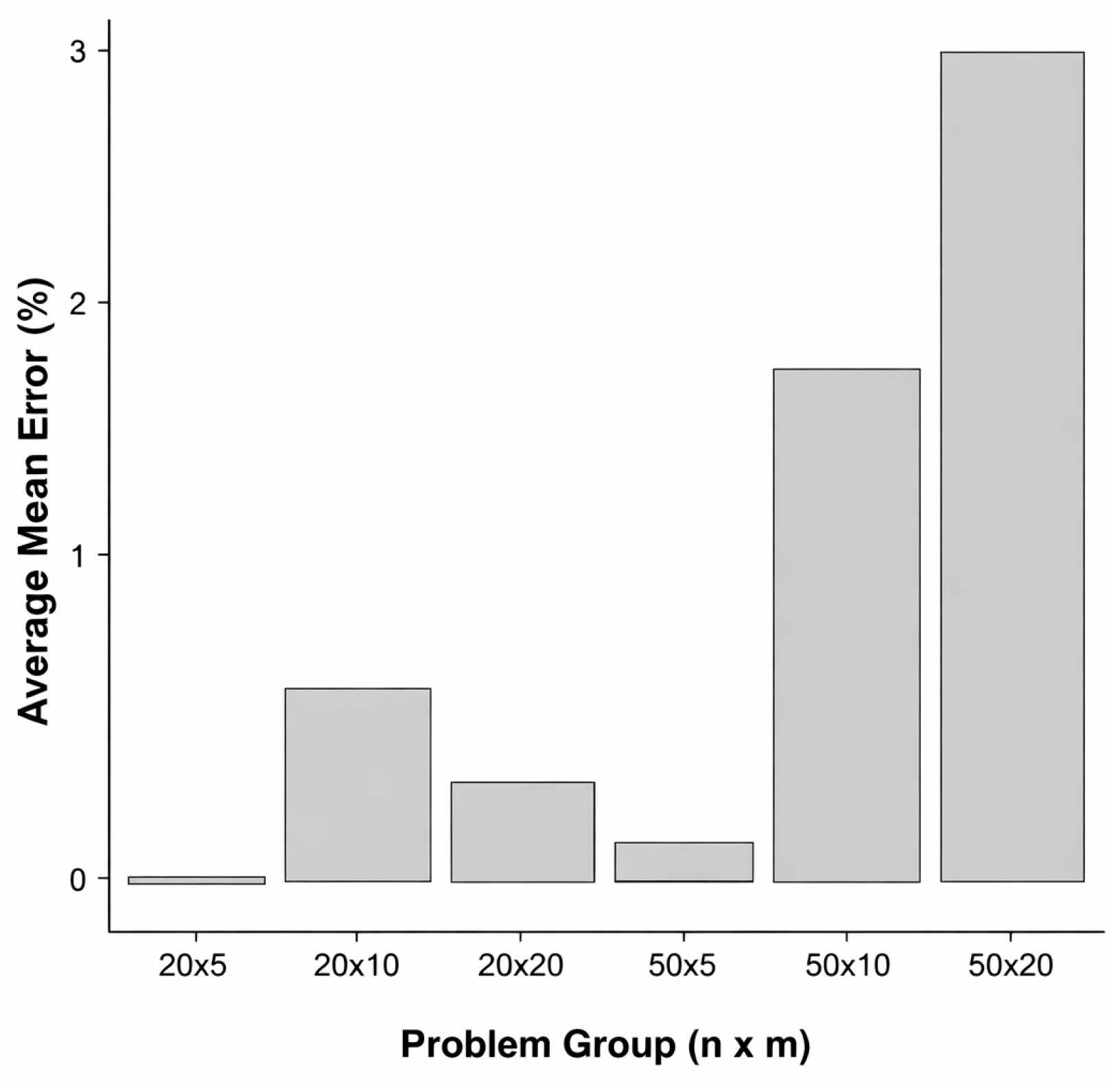
For a clearer comprehension of hybrid SSA’s performance in tackling the PFSP with makespan measure, Figure 4 shows the average mean error (%) on the y-axis, calculated as per Equation [6], while the x-axis depicts the instance set. Hybrid SSA demonstrates highly satisfactory average performance for the 20 × 5 and 50 × 5 instance set. For datasets with the highest complexity, represented by the last two sets, Figure 4 indicates an increase in the average mean error.

$$Average Mean Error(AME)={\displaystyle \frac{{\sum }_{i=1}^{10}M{E}_i}{10}}$$

(16)

where the Average Mean Error (AME) is calculated by averaging the mean errors within each instance set. Since each set comprises 10 instances, the total mean error for the set is divided by 10 to obtain the AME. Additional analysis of hybrid SSA’s robustness and effectiveness is carried out in subsequent sections, accompanied by statistical examination.

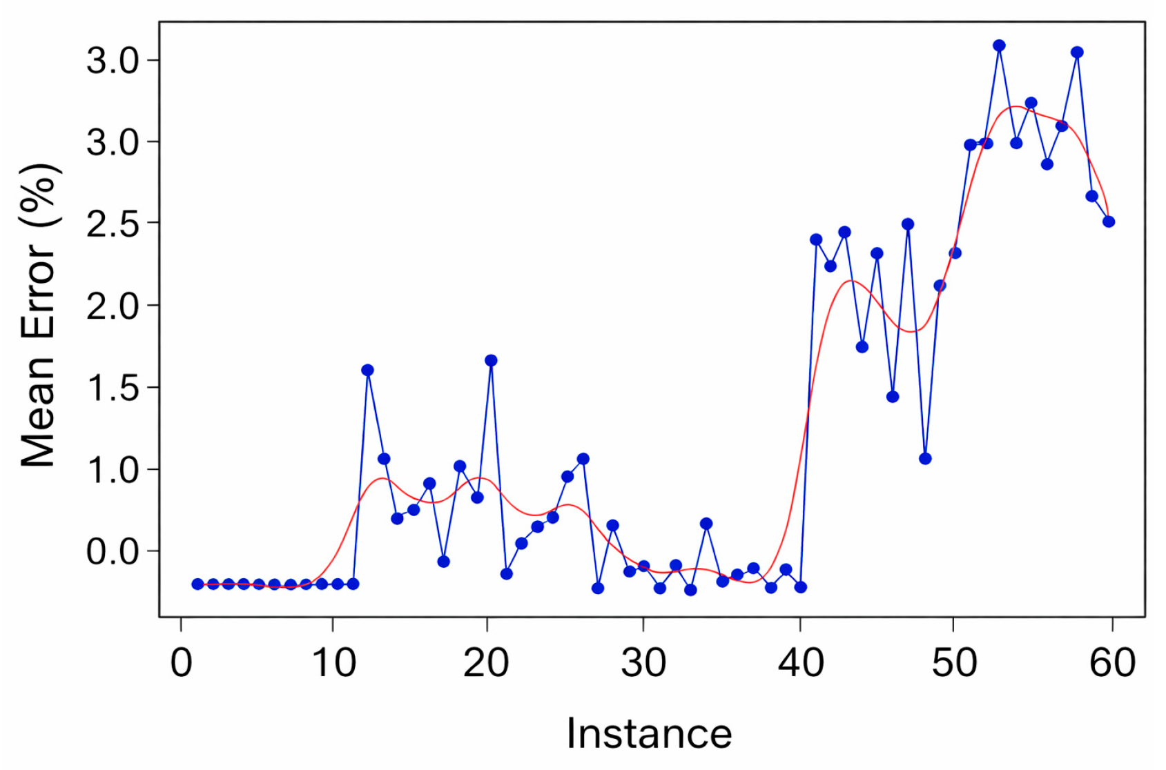
Figure 5 explicitly illustrates the progression of mean error with increasing instance complexity. The data show that the mean error remains relatively stable until the fourth instance set but escalates notably in the last two or more complex sets, as expected.

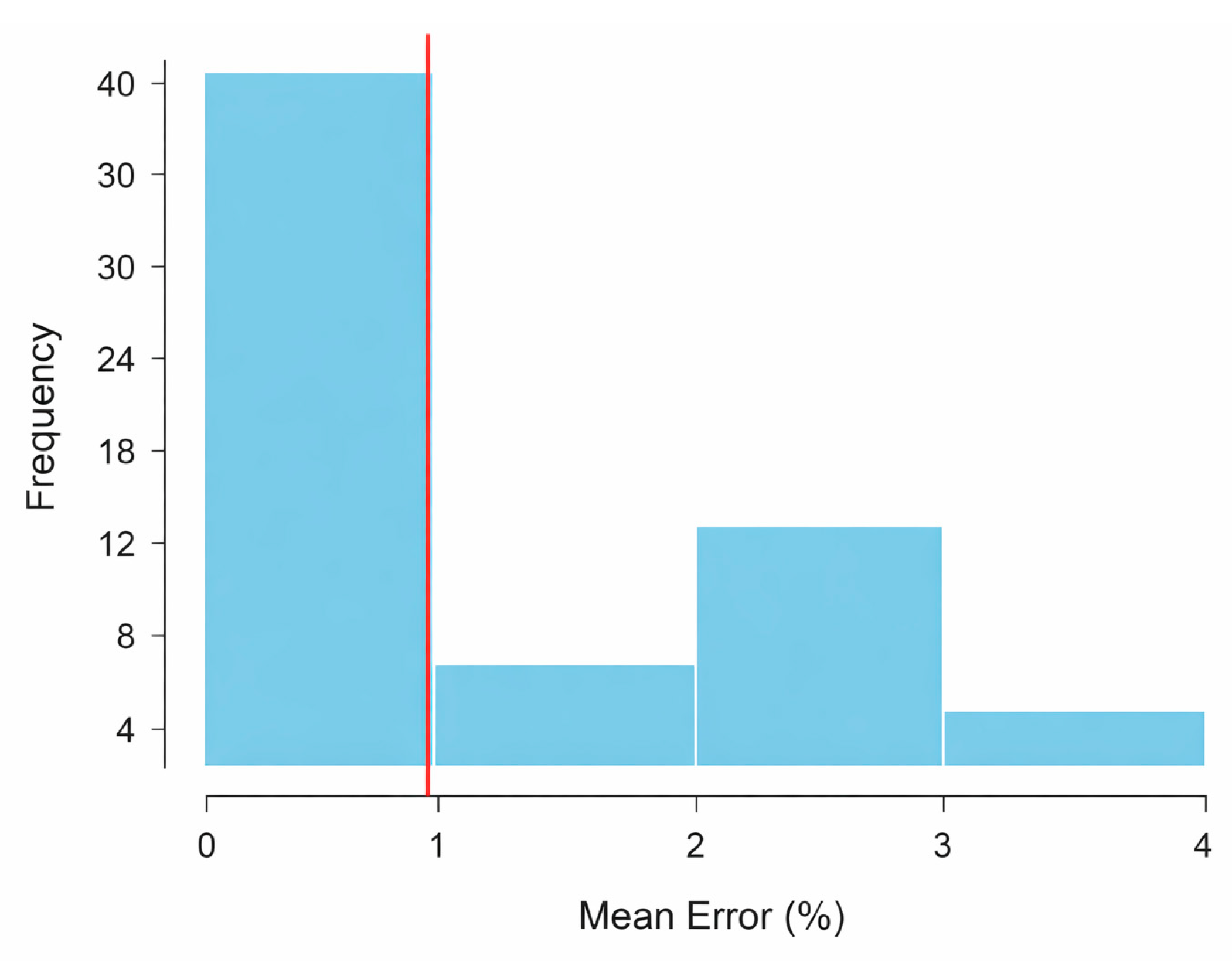
In Figure 6, the distribution of mean errors (%) for hybrid SSA is clearly depicted. The average mean error (%) is 0.99, as indicated by the line in the diagram. The majority of errors, 39 out of 60 (65%), fall between 0 and 1%. Five out of 60 mean errors (8.33%) are between 1% and 2%. Thirteen out of 60 (21.67%) fall within the range of 2% and 3%, while the remaining 5% of mean errors lie between 3% and 4%. The maximum mean error (%) value observed is 3.49.

5.2. Comparative Study: Hybrid SSA Against Other Hybrid Swarm Intelligence Metaheuristics

In order to ensure an objective study, seven swarm intelligence algorithms were integrated into the same framework as hybrid SSA, the GWO, WOA, TSO, FA, PSO, ABC, and BA. To ensure fair comparison, the Variable Neighborhood Search (VNS) and Path-Relinking procedures as described in Section 4.5 were employed as improvement mechanisms across all algorithms, resulting in the corresponding hybrid variants of GWO [63], WOA, TSO, FA, PSO, ABC, and BA. The population size was fixed at 100 individuals for all methods. Likewise, the initial population generation strategy (Section 4.4), as well as the encoding/decoding procedures, were kept identical for all methods. For each problem instance, the best makespan value was recorded across 10 independent runs. Finally, parameter sensitivity analyses were conducted for hybrid ABC and hybrid BA to identify parameter settings that yield the best performance.

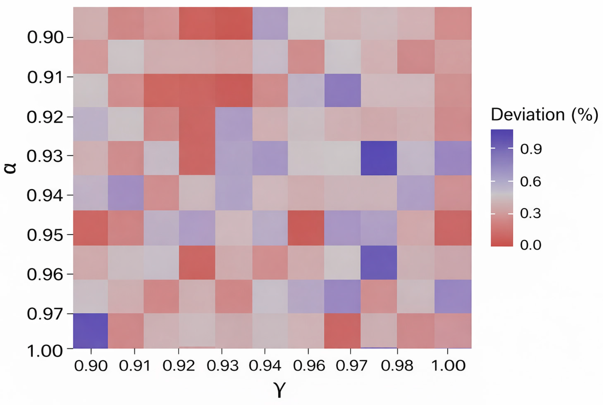
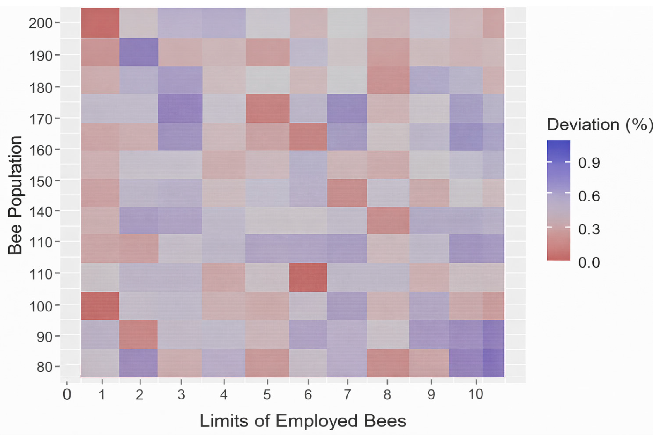
The hybrid BA has two significant parameters, namely α and γ. These parameters take values within the interval typically [0.9, 1]. In order to establish the optimal combination of α and γ, specifically for our problem, we perform an evaluation by measuring the mean error across different value sets for each parameter. For each combination, we conduct three trials, and the final deviation from the best-known solution (BKS) is calculated as the average of these trials. As shown in Figure 7, multiple sets of values achieve a lower mean error. In our study, we used the set [0.96, 0.96]. Similarly, for the hybrid ABC algorithm, two parameters were examined (as shown in Figure 8): the population size of the bees and the limit for the employed bees. In our study, we set the population of bees equal to 100, and the limit of the employed bees equal to 1.

As for the parameters of the remaining metaheuristics, we adopted recommended values from the literature. Specifically, in hybrid GWO [64] and hybrid WOA, the control parameter α was linearly decreased from 2 to 0 over the course of iterations. For hybrid PSO, the acceleration coefficients $c_1, c_{2 }$ were fixed at 2. In hybrid FA, $\beta$ and $\gamma$ were both set to 0.9. Finally, for hybrid TSO, parameters $z$ and $a$ were set to 0.05 and 0.7, respectively.

Table 2. Comparison results of AME for the PFSP with Tallard’s benchmark datasets (the bold formatting indicates the best values for each instances’ set while for AVG indicates its importance).

Instances’ Set	Hybrid SSA	Hybrid GWO	Hybrid TSO	Hybrid FA	Hybrid WOA	Hybrid PSO	Hybrid BA	Hybrid ABC
20 × 5	0.00	0.00	0.23	0.12	0.06	0.29	0.16	0.16
20 × 10	0.69	0.73	0.63	0.59	0.58	1.19	0.90	0.85
20 × 20	0.34	0.57	0.64	0.63	0.53	0.85	0.44	0.87
50 × 5	0.09	0.08	0.15	0.05	0.04	0.18	0.09	0.13
50 × 10	1.87	1.74	1.70	1.77	1.72	2.14	1.92	3.57
50 × 20	2.92	2.88	2.94	2.90	3.01	3.28	3.42	3.86
AVG	0.98	1.00	1.05	1.01	0.99	1.32	1.16	1.57

reports the average mean error (AME) for each Taillard instance set across all hybrid algorithms, while the AVG row summarizes the overall performance over the six instance sets. Overall, hybrid SSA achieves the best performance, presenting the lowest AVG value (0.98), followed by hybrid WOA (0.99) and hybrid GWO (1.00), indicating that these methods form the top-performing group on average.

Hybrid SSA and hybrid GWO [64] achieve zero error on the smaller instance set (20 × 5). On the 20 × 10 set, hybrid WOA presents the lowest AME (0.58), followed by hybrid FA (0.59) and hybrid SSA (0.69). In addition, hybrid SSA achieves the best AME on the 20 × 20 set (0.34) and clearly outperforms all competitors. For the 50 × 5 set, hybrid WOA yields the lowest AME (0.04), with hybrid FA also performing strongly (0.05), whereas hybrid SSA remains competitive (0.09). For the larger job sets, hybrid GWO and hybrid TSO provide the lowest AME on 50 × 10 (1.74 and 1.70, respectively), while hybrid GWO performs best on 50 × 20 (2.88), with hybrid SSA close behind (2.92). Regarding hybrid PSO, hybrid BA and hybrid ABC exhibit consistently higher errors, as reflected by their AVG values (1.32, 1.16, and 1.57, respectively), indicating weaker overall performance.

5.3. Statistical Analysis

5.3.1. Performance Comparison of Eight Hybrid SI Algorithms Using Box and Whisker Plots

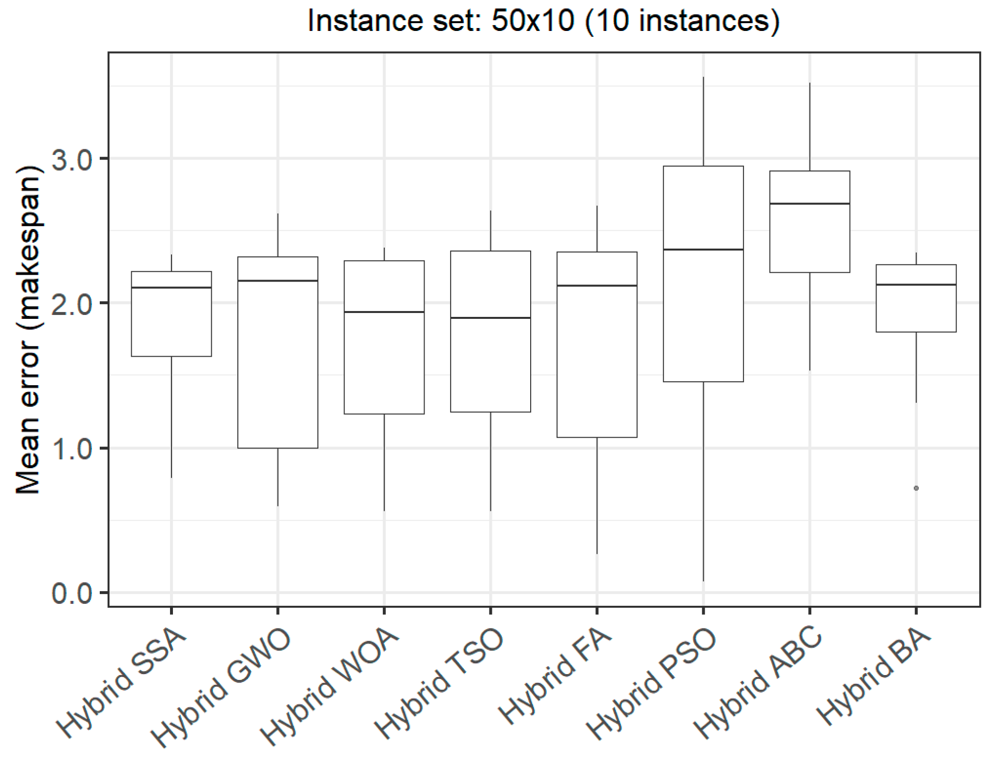
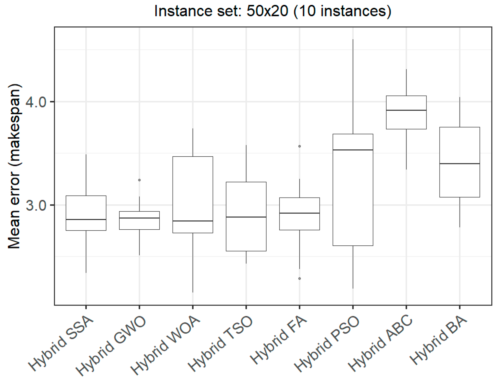
The performance of eight hybrid metaheuristics, namely the SSA, GWO, TSO, WOA, FA, PSO, ABC, and BA, was analyzed across 60 instances using box plots. These plots highlight each algorithm’s error trends, variability, and consistency over time. The box and whisker plots for every 10 instances reveal clear trends in the performance of the eight hybrid metaheuristics. In addition to the boxplot, descriptive statistics measures are computed for each hybrid method and instance set. Specifically, the mean and median errors, interquartile range (IQR), standard deviation (Std), and minimum/maximum values were used to provide a clearer interpretation of each algorithm’s robustness and stability. The complete set of descriptive statistics is reported in Appendix B (

Table A4. Descriptive statistic measures for each algorithm across every instance set.

Instance Set	Algorithm	Mean	Median	Std	IQR	Min	Max
20 × 5	Hybrid SSA	0.0000	0.0000	0.0000	0.0000	0.0000	0.0000
20 × 5	Hybrid GWO	0.0000	0.0000	0.0000	0.0000	0.0000	0.0000
20 × 5	Hybrid TSO	0.2100	0.0000	0.4698	0.1200	0.0000	1.4800
20 × 5	Hybrid FA	0.1240	0.0000	0.2995	0.0000	0.0000	0.9300
20 × 5	Hybrid WOA	0.0650	0.0000	0.2055	0.0000	0.0000	0.6500
20 × 5	Hybrid PSO	0.2900	0.0450	0.3827	0.5550	0.0000	1.0600
20 × 5	Hybrid BA	0.1590	0.0000	0.2576	0.3450	0.0000	0.5700
20 × 5	Hybrid ABC	0.1580	0.0000	0.3396	0.0000	0.0000	0.9300
20 × 10	Hybrid SSA	0.6870	0.6000	0.4946	0.3950	0.0000	1.5100
20 × 10	Hybrid GWO	0.7280	0.7050	0.4276	0.4675	0.0600	1.4300
20 × 10	Hybrid TSO	0.6890	0.6250	0.3370	0.4825	0.2900	1.2600
20 × 10	Hybrid FA	0.5920	0.5750	0.2553	0.3325	0.1300	0.9500
20 × 10	Hybrid WOA	0.5780	0.5650	0.4292	0.4550	0.0000	1.3200
20 × 10	Hybrid PSO	1.1890	1.1400	0.4564	0.6725	0.4200	1.8200
20 × 10	Hybrid BA	0.9000	1.0100	0.4757	0.6150	0.1900	1.3700
20 × 10	Hybrid ABC	0.8470	0.7700	0.5408	0.6950	0.0000	1.6300
20 × 20	Hybrid SSA	0.3450	0.3400	0.2833	0.3375	0.0000	0.8500
20 × 20	Hybrid GWO	0.5690	0.5650	0.2836	0.2350	0.2400	1.0500
20 × 20	Hybrid TSO	0.6340	0.5300	0.3038	0.2150	0.3600	1.1800
20 × 20	Hybrid FA	0.6340	0.4700	0.3569	0.4825	0.2300	1.2500
20 × 20	Hybrid WOA	0.5340	0.5550	0.2006	0.2900	0.2200	0.8300
20 × 20	Hybrid PSO	0.8510	0.6950	0.3968	0.6125	0.5500	1.3300
20 × 20	Hybrid BA	0.4370	0.4450	0.2652	0.3775	0.1000	0.8600
20 × 20	Hybrid ABC	0.8690	0.8500	0.3841	0.4050	0.5400	1.2900
50 × 5	Hybrid SSA	0.0870	0.0500	0.1230	0.1175	0.0000	0.4000
50 × 5	Hybrid GWO	0.0770	0.0000	0.1277	0.1175	0.0000	0.4000
50 × 5	Hybrid TSO	0.1350	0.0700	0.1394	0.2325	0.0000	0.3900
50 × 5	Hybrid FA	0.0510	0.0550	0.0479	0.0775	0.0000	0.1400
50 × 5	Hybrid WOA	0.0430	0.0150	0.0531	0.0775	0.0000	0.1400
50 × 5	Hybrid PSO	0.1810	0.1650	0.1470	0.1250	0.0300	0.4000
50 × 5	Hybrid BA	0.0950	0.0550	0.1059	0.1725	0.0000	0.3200
50 × 5	Hybrid ABC	0.1290	0.1500	0.0854	0.1000	0.0000	0.2600
50 × 10	Hybrid SSA	1.8670	2.1050	0.5220	0.5875	0.7900	2.3300
50 × 10	Hybrid GWO	1.7360	2.1500	0.7742	1.3275	0.5900	2.6200
50 × 10	Hybrid TSO	1.7740	1.8950	0.7082	1.1150	0.5600	2.6400
50 × 10	Hybrid FA	1.7710	2.1200	0.7859	1.2800	0.2600	2.6700
50 × 10	Hybrid WOA	1.7220	1.9350	0.6589	1.0600	0.5600	2.3800
50 × 10	Hybrid PSO	2.1430	2.3700	1.1230	1.4925	0.0700	3.5600
50 × 10	Hybrid BA	1.9190	2.1250	0.6023	0.4625	0.7200	2.3500
50 × 10	Hybrid ABC	2.5660	2.6850	0.8710	0.7025	1.5300	3.5200
50 × 20	Hybrid SSA	2.9170	2.8600	0.3649	0.3375	2.3400	3.4900
50 × 20	Hybrid GWO	2.8770	2.8700	0.1986	0.1750	2.5100	3.2400
50 × 20	Hybrid TSO	2.9390	2.8800	0.4384	0.6700	2.4800	3.5800
50 × 20	Hybrid FA	2.9020	2.9200	0.3411	0.3125	2.3800	3.5700
50 × 20	Hybrid WOA	3.0130	2.8450	0.5216	0.7375	2.1500	3.7400
50 × 20	Hybrid PSO	3.2810	3.5300	0.7819	1.0825	2.2800	4.6000
50 × 20	Hybrid BA	3.4150	3.4000	0.6227	0.6800	2.7800	4.0400
50 × 20	Hybrid ABC	3.8640	3.9150	0.4008	0.3200	3.3400	4.3100

).

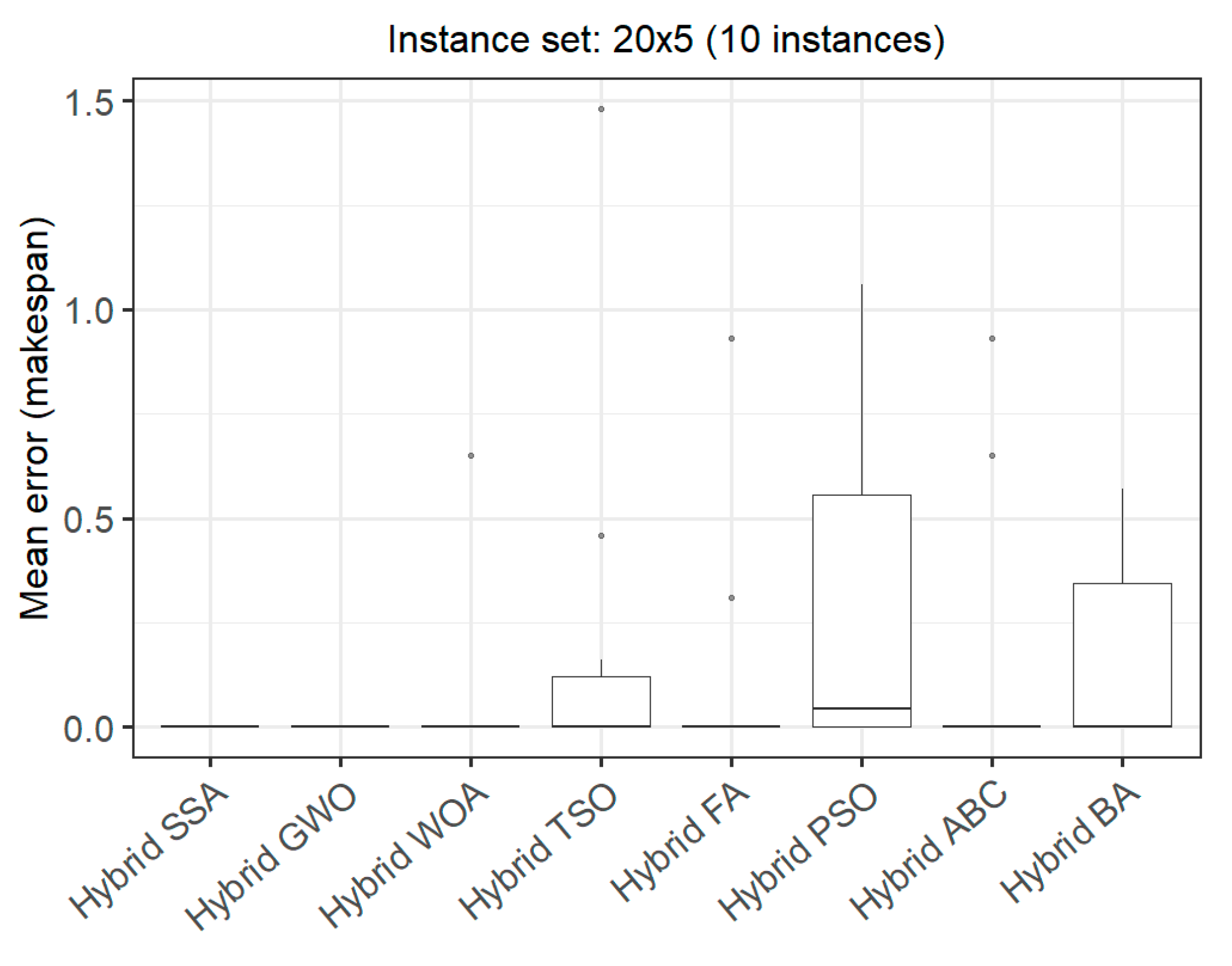
In the first 10 instances (Figure 9), hybrid SSA and hybrid GWO achieve zero error in all cases, reflecting perfectly consistent performance. Hybrid WOA, hybrid FA and hybrid ABC also exhibit zero median value. Occasional non-zero outcomes appear as upper tail outliers. In contrast, hybrid BA and hybrid TSO maintain a median of zero but show greater dispersion, suggesting less stable behavior that their competitors. Finally, hybrid PSO presents the weakest distribution in this set, with the highest median (0.0450), large IQR (0.5550) and a high maximum of 1.0600.

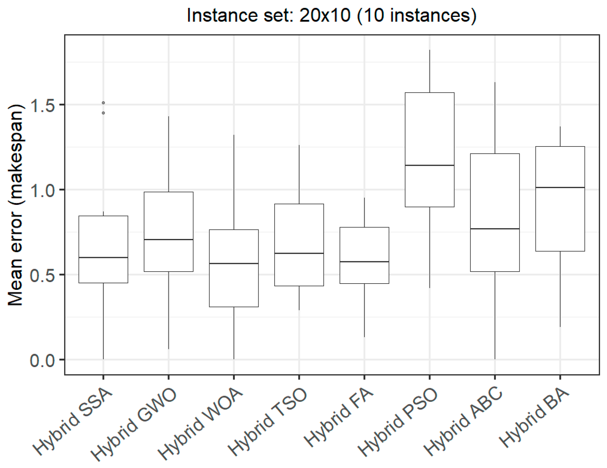
For the 20 × 10 set (Figure 10), hybrid WOA has the lowest median (0.5650) along with hybrid FA (0.5750) and relatively compact ranges, with hybrid FA appearing slightly more stable (IQR = 0.3325) than hybrid WOA (IQR = 0.4550). Hybrid SSA, hybrid TSO and hybrid GWO share similar medians (hybrid SSA: 0.6000, hybrid TSO: 0.6250, and hybrid GWO: 0.7050) and moderate dispersion. The weakest and least consistent performance for this set is provided by hybrid ABC, hybrid BA and finally, hybrid PSO, which exhibits the least favorable distribution.

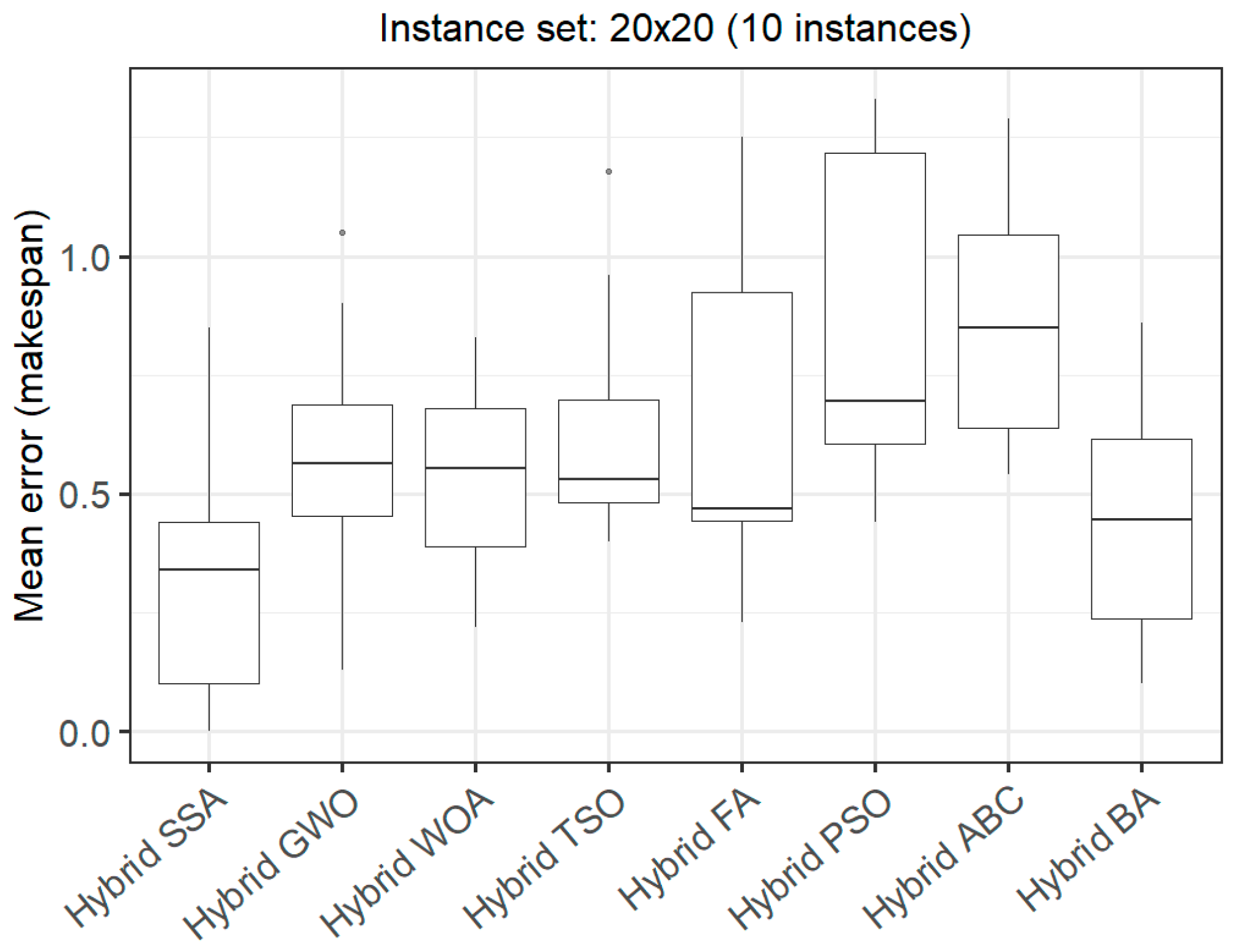
For the 20 × 20 instance set (Figure 11), hybrid SSA achieves the best distribution with the lowest median error (0.3400) and relatively small spread (IQR = 0.3375). Hybrid BA, hybrid GWO and hybrid WOA follow with higher medians ranging from 0.4450 to 0.5650 and moderate variability, while hybrid FA and hybrid TSO exhibit less favorable distributions and larger upper tails. Hybrid PSO and hybrid ABC perform worst, showing the highest medians (0.6950 and 0.8500) and consistently larger errors.

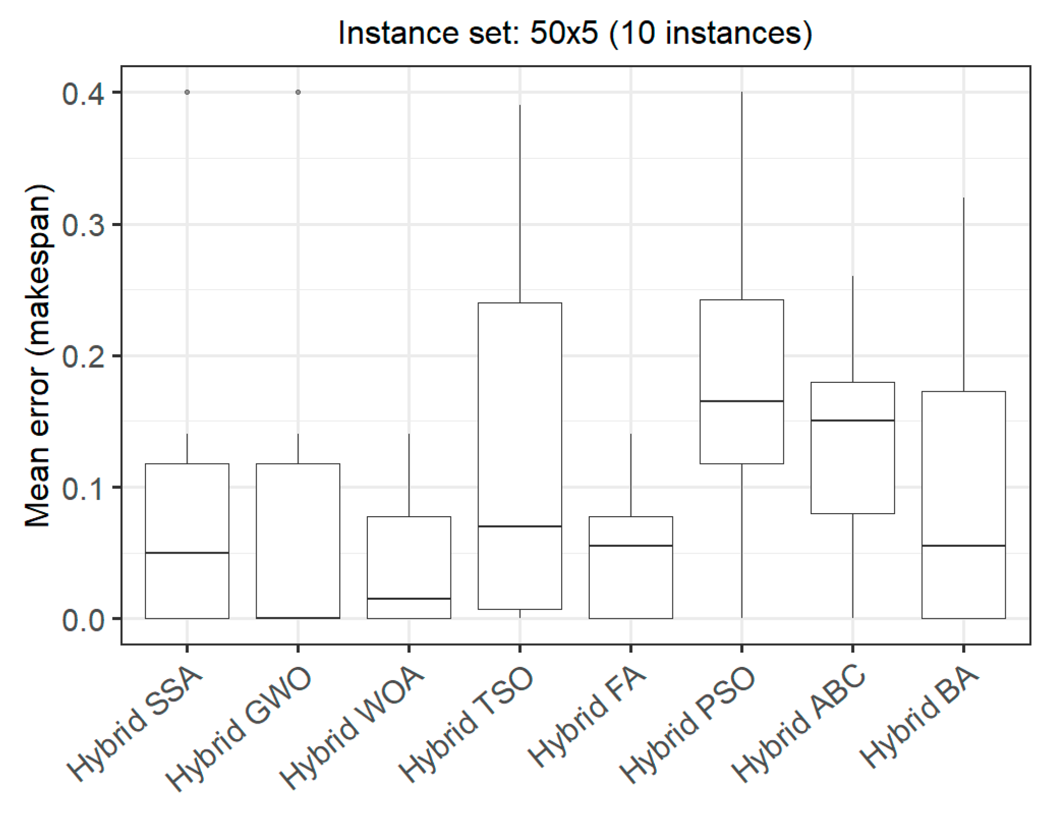
For the 50 × 5 instance set (Figure 12), hybrid WOA and hybrid FA provide the best and most stable performance, with very low medians and IQRs (0.0775 for both). Hybrid GWO and hybrid SSA remain competitive, showing many near-zero values but slightly wider dispersion. In particular, hybrid SSA achieves a low mean error (0.0870) and a median of 0.0500, indicating that it typically delivers near-zero errors on these instances. Hybrid BA, hybrid ABC, and hybrid TSO exhibit higher central errors and variability, whereas hybrid PSO performs worst, with the highest median (0.1650) and a generally elevated distribution.

For the 50 × 10 instance set (Figure 13), the best performing methods are hybrid WOA and hybrid TSO, with a median of 1.9350 and 1.8950, respectively. Hybrid SSA remains competitive with controlled variability (IQR = 0.5875), a moderate median of 2.1050 and the lowest maximum error among all methods, suggesting that hybrid SSA delivers more consistent performance and avoids extreme worst-case outcomes on the 50 × 10 instance set. Hybrid GWO and FA follow next with median of 2.1500 and 2.1200, respectively, although hybrid FA exhibits slightly smaller spread (IQR = 1.2800) than hybrid GWO (IQR = 1.3275). Hybrid PSO, hybrid ABC and hybrid BA consistently perform worst with higher medians and dispersion.

For the 50 × 20 instance set (Figure 14), hybrid SSA achieves strong performance, with a mean error of 2.9170 and a median of 2.8600, placing it close to the best methods in this group. However, hybrid GWO exhibits a slightly lower mean (2.8770) and dispersion (IQR = 0.1750), indicating superior stability. Compared to other competitors, hybrid SSA shows moderate variability (IQR = 0.3375) and a bounded upper tail (max = 3.4900), performing better than hybrid WOA and substantially better than the weaker methods (hybrid PSO, hybrid BA, and hybrid ABC) that display higher central errors and wider spreads.

5.3.2. Statistical Analysis with Non-Parametric Tests

We implemented several methods of statistical testing along with post-hoc analyses, namely the Friedman, aligned Friedman and Quade tests, using multiple p-value adjustment procedures (Bonfferroni, Holm, FDR-BY, Sidak, FDR-BH, and Hommel). In addition, we report the Kruskal–Wallis test and complemented with Wilcoxon based pairwise comparisons with multiple-comparison corrections. Together, these methods provide a more robust assessment of performance differences between the tested algorithms and help support more reliable conclusions.

Table 3. Average rankings for Friedman, aligned Friedman, and Quade tests (The best (smaller) obtained rankings are highlighted in bold.).

Method	Friedman	Aligned Friedman	Quade
Hybrid WOA	3.5417	186.2667	3.3791
Hybrid SSA	3.5917	176.8917	3.5026
Hybrid FA	3.7917	196.3750	3.7447
Hybrid GWO	3.8417	188.5000	3.7131
Hybrid TSO	4.3750	221.1583	4.0933
Hybrid BA	4.6250	264.4417	4.9048
Hybrid PSO	6.0750	339.1667	5.9999
Hybrid ABC	6.1583	351.2000	6.6626

reports the average ranks obtained from Friedman, aligned Friedman and Quade tests, where smaller values indicate higher relative performance. Hybrid WOA ranks first in two tests (Friedman: 3.5417, Quade: 3.3791), while hybrid SSA achieves very similar performance and ranks first in the Aligned Friedman test. Hybrid GWO and hybrid FA follow closely, although they rank slightly lower across the three tests. Hybrid TSO and hybrid BA form the next performance tier, whereas hybrid PSO and hybrid ABC exhibit the weakest relative performance. These findings are supported by the omnibus tests (

Table 4. Omnibus tests for statistic F and p-value (p < 0.05 significant difference).

Measure	Friedman	Aligned Friedman	Quade
Statistic F	1.767 × 101	1.767 × 101	1.767 × 101
p-value	1.591 × 10−20	1.591 × 10−20	1.591 × 10−20

), where all three methods (Friedman, Aligned Friedman and Quade test) indicate statistically significant differences among the algorithms.

To determine whether the control algorithm (hybrid SSA in this case) differs statistically from any other algorithm we performed, for each test, a post-hoc analysis against the control was performed, using multiple p-value adjustment procedures.

Table 5. Post-hoc analysis using multiple p-value adjustment procedures for Friedman test.

Hybrid SSA vs.	Bonferroni	Holm	FDR-BY	SIDAK	FDR-BH	Hommel
Hybrid GWO	1	1	1	9.905 × 10−1	6.732 × 10−1	8.891 × 10−1
Hybrid TSO	2.055 × 10−1	1.174 × 10−1	1.332 × 10−1	1.8825 × 10−1	5.1372 × 10−2	1.1742 × 10−1
Hybrid WOA	1	1	1	9.9999 × 10−1	8.8908 × 10−1	8.8908 × 10−1
Hybrid FA	1	1	1	9.9757 × 10−1	6.7317 × 10−1	8.8908 × 10−1
Hybrid PSO	1.130 × 10−10	9.690 × 10−11	1.466 × 10−10	1.130 × 10−10	5.652 × 10−11	9.690 × 10−11
Hybrid ABC	2.544 × 10−11	2.544 × 10−11	6.597 × 10−11	2.544 × 10−11	2.544 × 10−11	2.544 × 10−11
Hybrid BA	2.892 × 10−2	2.066 × 10−2	2.500 × 10−2	2.857 × 10−2	9.640 × 10−3	2.066 × 10−2

reports Friedman’s post-hoc results. Statistically significant differences (p < 0.05) are observed between hybrid SSA and hybrid variants of PSO, ABC, and BA across all p-value adjustment procedures. In contrast, no statistically significant differences are detected between hybrid SSA and hybrid variants of GWO, WOA, FA or TSO, although the comparison with hybrid TSO is close to 0.05 threshold under FDR-BH.

In Appendix B,

Table A2. Post-hoc analysis using multiple p-value adjustment procedures for Aligned Friedman test.

Hybrid SSA vs.	Bonferroni	Holm	FDR-BY	SIDAK	FDR-BH	Hommel
Hybrid GWO	1	1	1	9.9048 × 10−1	6.7317 × 10−1	8.8908 × 10−1
Hybrid TSO	2.05548 × 10−1	1.1742 × 10−1	1.3320 × 10−1	1.8825 × 10−1	5.1372 × 10−2	1.1742 × 10−1
Hybrid WOA	1	1	1	9.9999 × 10−1	8.8908 × 10−1	8.8908 × 10−1
Hybrid FA	1	1	1	9.9757 × 10−1	6.7317 × 10−1	8.8908 × 10−1
Hybrid PSO	1.1304 × 10−10	9.6896 × 10−11	1.4655 × 10−10	1.1304 × 10−10	5.6522 × 10−11	9.6896 × 10−11
Hybrid ABC	2.5443 × 10−11	2.5442 × 10−11	6.5969 × 10−11	2.5443 × 10−11	2.5442 × 10−11	2.5442 × 10−11
Hybrid BA	2.8921 × 10−2	2.0658 × 10−2	2.4996 × 10−2	2.8565 × 10−2	9.6404 × 10−3	2.0658 × 10−2

and

Table A3. Post-hoc analysis using multiple p-value adjustment procedures for Quade test.

Hybrid SSA vs.	Bonferroni	Holm	FDR-BY	SIDAK	FDR-BH	Hommel
Hybrid GWO	1	1	1	0.9993	0.7527	0.7870
Hybrid TSO	1	0.7867	0.8924	0.7841	0.3442	0.7867
Hybrid WOA	1	1	1	1	0.7870	0.7870
Hybrid FA	1	1	1	0.9983	0.7527	0.7870
Hybrid PSO	5.5552 × 10−7	4.7616 × 10−7	7.2019 × 10−7	5.5552 × 10−7	2.7776 × 10−7	4.7616 × 10−7
Hybrid ABC	1.2287 × 10−10	1.2287 × 10−10	3.1858 × 10−10	1.2287 × 10−10	1.2287 × 10−10	1.2287 × 10−10
Hybrid BA	0.0160	0.0114	0.0138	0.0159	0.0053	0.0114

present the post-hoc results for the aligned Friedman test with multiple p-value adjustment procedures, while Table A3 reports the results for Quade’s test. The aligned Friedman post-hoc results, presented in Table A2, are consistent with Friedman’s analysis. Statistically significant differences (p < 0.05) are found between hybrid SSA and hybrid variants of PSO, ABC, and BA, whereas no statistically significant differences were observed with all the other algorithms. Similarly, Quade’s post-hoc analysis (Table A3) confirms the same hypothesis.

Overall, hybrid SSA demonstrates consistently high relative performance and ranks among the best-performing groups. Post-hoc analyses show that it significantly outperforms the weaker algorithms (hybrid variants of PSO, ABC, and BA), while its performance is statistically indistinguishable from the other top competitors (hybrid variants of WOA, GWO, FA, and TSO).

Table 6. Kruskal-Wallis Omnibus test.

Test	Chi-Squared	df	p-Value
Kruskal–Wallis	9.1086	7	0.245

presents the results for the Kruskal–Wallis test. Kruskal–Walis test is reported as complementary analysis, since the computational experiments were conducted on the same benchmark instances. According to the findings, there is no significant difference among the algorithms ($X^2$ = 9.1086, and p = 0.245 > 0.05). Therefore, based on the omnibus test, we fail to reject the null hypothesis of equal performance distributions across methods. However, since the study follows a blocked design (same instances across algorithms), the primary omnibus results are provided by Friedman-type tests, which indicate significant differences among methods.

Wilcoxon signed-rank post-hoc comparisons against hybrid SSA (

Table 7. Wilcoxon signed-rank post-hoc comparisons against control.

Hybrid SSA vs.	Hybrid GWO	Hybrid TSO	Hybrid WOA	Hybrid FA	Hybrid PSO	Hybrid ABC	Hybrid BA
Raw-p	0.2340	0.0427	0.3044	0.1774	1.972 × 10−6	9.894 × 10−8	2.509 × 10−4
Bonferroni	1	0.2992	1	1	1.381 × 10−5	6.926 × 10−7	0.0018
Holm	0.5322	0.1710	0.5322	0.5322	1.183 × 10−5	6.926 × 10−7	0.0013
FDR-BH	0.2730	0.0748	0.3044	0.2484	6.903 × 10−6	6.926 × 10−7	5.853 × 10−4
FDR-BY	0.7077	0.1940	0.7891	0.6440	1.790 × 10−5	1.796 × 10−6	0.0015
SIDAK	0.8452	0.2635	0.9212	0.7452	1.381 × 10−5	6.926 × 10−7	0.0018
Hommel	0.3044	0.1710	0.3044	0.3044	1.183 × 10−5	6.926 × 10−7	0.0013
Median Difference	0.0000	−0.0150	0.0000	0.0000	−0.2050	−0.3450	−0.0550
Mean Difference	−0.0140	−0.0797	−0.0087	−0.0285	−0.3387	−0.4217	−0.1703
Wins	24	30	19	26	40	41	31
Ties	20	13	19	18	10	13	14
Losses	16	17	22	16	10	6	15

) with multiple p-value procedures indicate that hybrid SSA achieves statistically significant improvements over hybrid variants of PSO, ABC and, BA, as all p-adjusted values remain below threshold across every correction method (Bonferroni, Holm, FDR-BH, FDR-BY, Sidak, and Hommel). Mean and median differences also suggest that hybrid SSA outperforms these algorithms. In addition, hybrid SSA wins in 40 instances, hybrid PSO in 41, and hybrid ABC and hybrid BA in 31, which are more than 50% of all instances.

In contrast, no statistically significant differences are detected between hybrid SSA and the stronger competitors’ hybrid variants of GWO, WOA, TSO, and FA, which are consistent with the previous findings. In terms of win-loss counts, hybrid SSA outperforms hybrid GWO on 24 instances (40.0% of all instances) and is outperformed on 16 instances with 20 ties. Against hybrid TSO, hybrid SSA records 30 wins (50.0%) and 17 losses with 13 ties. Similarly, hybrid SSA achieves 26 wins (43.3%) over hybrid FA and 16 losses, with 18 ties. For hybrid WOA, the comparison is nearly balanced, and hybrid WOA loses on 22 instances and wins on 19, while 19 instances result in identical errors (ties). Generally, hybrid SSA presents small advances in terms of mean differences (negative values) and exhibits equal (zero value) or improved (negative) median differences compared with the other algorithms.

6. Conclusions and Future Research Directions

The comparative evaluation on Taillard benchmark instances shows that hybrid SSA achieves the lowest overall average mean error. The Friedman, aligned Friedman and Quade omnibus tests report highly significant results, confirming that the observed performance differences are not random. Consequently, post-hoc comparisons against the control algorithm (hybrid SSA) were conducted. Post-hoc analysis revealed that hybrid SSA differs significantly from the weakest methods, including hybrid variants of PSO, ABC, and BA. These findings are consistent with all p-value adjustment procedures and strong win-tie-loss counts, provided by the Wilcoxon procedure. In contrast, no statistically significant differences are detected between hybrid SSA and the strongest competitors (hybrid variants of GWO, WOA, FA, and TSO) after multiple-comparison correction, indicating these approaches form a statistical equivalent set. However, in terms of the number of instances with lower mean error values, hybrid SSA remains superior to all other hybrid methods except for hybrid WOA. In direct comparison between the two methods, Hybris SSA performs better in 19 instances, whereas Hybris WOA performs better in 22. Although the Kruskal–Willis omniums test did not indicate statistically significant overall differences among the methods, this result is reported only as a supplementary analysis, since all algorithms were evaluated on the same benchmark instances. The primary inferential evidence is therefore provided by Friedman, Aligned Friedman, and Quade tests, which are more suitable for a related sample design. Further statistical analysis based on box plots and descriptive statistical measures shows that hybrid SSA exhibits comparatively low dispersion and among the lowest variability levels, indicating consistent and stable behavior across all instances. Overall, hybrid SSA can be considered an efficient solution method for the PFSP, since it achieves the lower average mean error and demonstrates stable performance across the test data compared with the other methods examined in this study.

A potential future goal following this study could be to extend hybrid SSA to address other complex scheduling problems, such as multi-objective PFSP, stochastic PFSP, or PFSP with sequence-dependent setup times. Another avenue could involve integrating the proposed algorithm with machine learning techniques to dynamically adapt its parameters based on the problem instance characteristics. Additionally, further research could explore parallel or distributed implementations of the algorithm to handle larger-scale problems more efficiently.

Limitations of this study arise from preliminary analysis of the hybrid initialization ratio set at 70% randomized NEH and 30% random solutions. Since this is a critical component of the proposed framework, a more comprehensive sensitivity analysis will be caried out in future work. In addition, future research will examine large-scale Taillard instances more extensively in order to further evaluate the robustness of the parameter settings, such as producer-scrounger ratio, ST, and R2 combination.

References

1. Mirjalili, S.; Mirjalili, S.M.; Lewis, A. Grey Wolf Optimizer. Adv. Eng. Softw. 2014, 69, 46–61. [Google Scholar] [CrossRef]
2. Xue, J.; Shen, B. A novel swarm intelligence optimization approach: Sparrow search algorithm. Syst. Sci. Control Eng. 2020, 8, 22–34. [Google Scholar] [CrossRef]
3. Nasser, A.; Zaied, H.; Ismail, M.M.; Mohamed, S.S. Permutation Flow Shop Scheduling Problem with Makespan Criterion: Literature Review. J. Theor. Appl. Inf. Technol. 2021, 28, 830–848. Available online: www.jatit.org (accessed on 1 April 2026).
4. Chen, H.; Ma, X.; Huang, S. A Feature Selection Method for Intrusion Detection Based on Parallel Sparrow Search Algorithm. In Proceedings of the 2021 16th International Conference on Computer Science & Education (ICCSE); IEEE: Piscataway, NJ, USA, 2021; pp. 685–690. [Google Scholar] [CrossRef]
5. Zheng, Y.; Liu, F. Optimal Dispatch Strategy of Microgrid Energy Storage Based on Improved Sparrow Search Algorithm. In Proceedings of the 2021 40th Chinese Control Conference (CCC); IEEE: Piscataway, NJ, USA, 2021; pp. 1832–1837. [Google Scholar] [CrossRef]
6. Wu, M.; Yang, D.; Yang, Z.; Guo, Y. Sparrow Search Algorithm for Solving Flexible Jobshop Scheduling Problem. In Advances in Swarm Intelligence: Proceedings of the 12th International Conference, ICSI 2021; Tan, Y., Shi, Y., Eds.; Springer International Publishing: Cham, Switzerland, 2021; pp. 140–154. [Google Scholar]
7. Tang, A.; Zhou, H.; Han, T.; Xie, L. A Chaos Sparrow Search Algorithm with Logarithmic Spiral and Adaptive Step for Engineering Problems. Comput. Model. Eng. Sci. 2022, 130, 331–364. [Google Scholar] [CrossRef]
8. Salam, M.A.; Azar, A.T.; Hussien, R. An Improved Sparrow Search Algorithm for Node Localization in WSN. Comput. Mater. Contin. 2022, 71, 2037–2051. [Google Scholar] [CrossRef]
9. Awadallah, M.A.; Al-Betar, M.A.; Doush, I.A.; Makhadmeh, S.N.; Al-Naymat, G. Recent Versions and Applications of Sparrow Search Algorithm. Arch. Comput. Methods Eng. 2023, 30, 2831–2858. [Google Scholar] [CrossRef]
10. Garey, M.R.; Johnson, D.S.; Sethi, R. The Complexity of Flowshop and Jobshop Scheduling. Math. Oper. Res. 1976, 1, 117–129. [Google Scholar] [CrossRef]
11. Hansen, P.; Mladenović, N. Variable neighborhood search: Principles and applications. Eur. J. Oper. Res. 2001, 130, 449–467. [Google Scholar] [CrossRef]
12. Glover, F.; Laguna, M.; Marti, R. Scatter Search and Path Relinking: Advances and Applications. In Handbook of Metaheuristics; Glover, F., Kochenberger, G.A., Eds.; Springer: Boston, MA, USA, 2003; pp. 1–35. [Google Scholar] [CrossRef]
13. Nawaz, M.; Enscore, E.E.; Ham, I. A heuristic algorithm for the m-machine, n-job flow-shop sequencing problem. Omega 1983, 11, 91–95. [Google Scholar] [CrossRef]
14. Xie, L.; Han, T.; Zhou, H.; Zhang, Z.-R.; Han, B.; Tang, A. Tuna Swarm Optimization: A Novel Swarm-Based Metaheuristic Algorithm for Global Optimization. Comput. Intell. Neurosci. 2021, 2021, 9210050. [Google Scholar] [CrossRef]
15. Mirjalili, S.; Lewis, A. The Whale Optimization Algorithm. Adv. Eng. Softw. 2016, 95, 51–67. [Google Scholar] [CrossRef]
16. Yang, X.-S. Firefly Algorithms for Multimodal Optimization. In Stochastic Algorithms: Foundations and Applications: Proceedings fo the 5th International Symposium, SAGA 2009; Watanabe, O., Zeugmann, T., Eds.; Springer: Berlin/Heidelberg, Germany, 2009; pp. 169–178. [Google Scholar]
17. Kennedy, J.; Eberhart, R. Particle swarm optimization. In Proceedings of ICNN’95—International Conference on Neural Networks; IEEE: Piscataway, NJ, USA, 1995; Volume 4, pp. 1942–1948. [Google Scholar] [CrossRef]
18. Yang, X.-S. A New Metaheuristic Bat-Inspired Algorithm. In Nature Inspired Cooperative Strategies for Optimization (NICSO 2010); González, J.R., Pelta, D.A., Cruz, C., Terrazas, G., Krasnogor, N., Eds.; Springer: Berlin/Heidelberg, Germany, 2010; pp. 65–74. [Google Scholar] [CrossRef]
19. Karaboga, D.; Basturk, B. A powerful and efficient algorithm for numerical function optimization: Artificial bee colony (ABC) algorithm. J. Glob. Optim. 2007, 39, 459–471. [Google Scholar] [CrossRef]
20. Taillard, E. Benchmarks for basic scheduling problems. Eur. J. Oper. Res. 1993, 64, 278–285. [Google Scholar] [CrossRef]
21. Li, X.; Ma, X.; Xiao, F.; Xiao, C.; Wang, F.; Zhang, S. Time-series production forecasting method based on the integration of Bidirectional Gated Recurrent Unit (Bi-GRU) network and Sparrow Search Algorithm (SSA). J. Pet. Sci. Eng. 2022, 208, 109309. [Google Scholar] [CrossRef]
22. Song, C.; Yao, L.; Hua, C.; Ni, Q. A novel hybrid model for water quality prediction based on synchrosqueezed wavelet transform technique and improved long short-term memory. J. Hydrol. 2021, 603, 126879. [Google Scholar] [CrossRef]
23. Ahmed, A.N.; Van Lam, T.; Hung, N.D.; Van Thieu, N.; Kisi, O.; El-Shafie, A. A comprehensive comparison of recent developed meta-heuristic algorithms for streamflow time series forecasting problem. Appl. Soft Comput. 2021, 105, 107282. [Google Scholar] [CrossRef]
24. Gai, J.; Zhong, K.; Du, X.; Yan, K.; Shen, J. Detection of gear fault severity based on parameter-optimized deep belief network using sparrow search algorithm. Measurement 2021, 185, 110079. [Google Scholar] [CrossRef]
25. Zhang, Z.; Han, Y. Discrete sparrow search algorithm for symmetric traveling salesman problem. Appl. Soft Comput. 2022, 118, 108469. [Google Scholar] [CrossRef]
26. Xue, J.; Shen, B.; Pan, A. A hierarchical sparrow search algorithm to solve numerical optimization and estimate parameters of carbon fiber drawing process. Artif. Intell. Rev. 2023, 56, 1113–1148. [Google Scholar] [CrossRef]
27. Tao, X.; Liu, Z.; Zhao, F.; Lan, R.; Liu, R.; Fu, L.; Ouyang, Y. An SSA-LC-DAE Method for Extracting Network Security Elements. IEEE Trans. Netw. Sci. Eng. 2023, 10, 1175–1185. [Google Scholar] [CrossRef]
28. Wu, H.; Zhang, A.; Han, Y.; Nan, J.; Li, K. Fast stochastic configuration network based on an improved sparrow search algorithm for fire flame recognition. Knowl.-Based Syst. 2022, 245, 108626. [Google Scholar] [CrossRef]
29. Wang, Z.; Sun, G.; Zhou, K.; Zhu, L. A parallel particle swarm optimization and enhanced sparrow search algorithm for unmanned aerial vehicle path planning. Heliyon 2023, 9, e14784. [Google Scholar] [CrossRef] [PubMed]
30. Yang, L.; Li, Z.; Wang, D.; Miao, H.; Wang, Z. Software Defects Prediction Based on Hybrid Particle Swarm Optimization and Sparrow Search Algorithm. IEEE Access 2021, 9, 60865–60879. [Google Scholar] [CrossRef]
31. Li, H.; Zhang, B.; Li, J.; Zheng, T.; Yang, H. Using Sparrow Search Hunting Mechanism to Improve Water Wave Algorithm. In Proceedings of the 2021 IEEE International Conference on Progress in Informatics and Computing (PIC); IEEE: Piscataway, NJ, USA, 2021; pp. 19–23. [Google Scholar] [CrossRef]
32. Shi, L.; Ding, X.; Li, M.; Liu, Y. Research on the Capability Maturity Evaluation of Intelligent Manufacturing Based on Firefly Algorithm, Sparrow Search Algorithm, and BP Neural Network. Complexity 2021, 2021, 5554215. [Google Scholar] [CrossRef]
33. Huang, S.; Huang, H. A Novel Whale Optimization Algorithm with Sparrow algorithm and Golden Sine Leading Strategy. In Proceedings of the 2021 5th Asian Conference on Artificial Intelligence Technology (ACAIT); IEEE: Piscataway, NJ, USA, 2021; pp. 113–122. [Google Scholar] [CrossRef]
34. Fadheel, B.A.; Wahab, N.I.A.; Mahdi, A.J.; Premkumar, M.; Radzi, M.A.B.M.; Che Soh, A.B.; Veerasamy, V.; Irudayaraj, A.X.R. A Hybrid Grey Wolf Assisted-Sparrow Search Algorithm for Frequency Control of RE Integrated System. Energies 2023, 16, 1177. [Google Scholar] [CrossRef]
35. Yao, Y.; Lei, S.; Guo, Z.; Li, Y.; Ren, S.; Liu, Z.; Guan, Q.; Luo, P. Fast optimization for large scale logistics in complex urban systems using the hybrid sparrow search algorithm. Int. J. Geogr. Inf. Sci. 2023, 37, 1420–1448. [Google Scholar] [CrossRef]
36. Khaleel, M.I. Efficient job scheduling paradigm based on hybrid sparrow search algorithm and differential evolution optimization for heterogeneous cloud computing platforms. Internet Things 2023, 22, 100697. [Google Scholar] [CrossRef]
37. Storn, R. On the usage of differential evolution for function optimization. In Proceedings of North American Fuzzy Information Processing; IEEE: Berkeley, CA, USA, 1996; pp. 519–523. [Google Scholar] [CrossRef]
38. Storn, R. System design by constraint adaptation and differential evolution. IEEE Trans. Evol. Comput. 1999, 3, 22–34. [Google Scholar] [CrossRef]
39. Gharehchopogh, F.S.; Namazi, M.; Ebrahimi, L.; Abdollahzadeh, B. Advances in Sparrow Search Algorithm: A Comprehensive Survey. Arch. Comput. Methods Eng. 2023, 30, 427–455. [Google Scholar] [CrossRef]
40. Zhang, C.; Ding, S. A stochastic configuration network based on chaotic sparrow search algorithm. Knowl.-Based Syst. 2021, 220, 106924. [Google Scholar] [CrossRef]
41. Chen, X.; Huang, X.; Zhu, D.; Qiu, Y. Research on chaotic flying sparrow search algorithm. J. Phys. Conf. Ser. 2021, 1848, 012044. [Google Scholar] [CrossRef]
42. Liu, G.; Shu, C.; Liang, Z.; Peng, B.; Cheng, L. A Modified Sparrow Search Algorithm with Application in 3d Route Planning for UAV. Sensors 2021, 21, 1224. [Google Scholar] [CrossRef]
43. Chen, D.; Zhao, J.; Huang, P.; Deng, X.; Lu, T. An improved sparrow search algorithm based on levy flight and opposition-based learning. Assem. Autom. 2021, 41, 697–713. [Google Scholar] [CrossRef]
44. Jia, J.; Yuan, S.; Shi, Y.; Wen, J.; Pang, X.; Zeng, J. Improved sparrow search algorithm optimization deep extreme learning machine for lithium-ion battery state-of-health prediction. iScience 2022, 25, 103988. [Google Scholar] [CrossRef]
45. Chang, Z.; Gu, Q.; Lu, C.; Zhang, Y.; Ruan, S.; Jiang, S. 5G Private Network Deployment Optimization Based on RWSSA in Open-Pit Mine. IEEE Trans. Ind. Inform. 2022, 18, 5466–5476. [Google Scholar] [CrossRef]
46. Tang, Y.; Dai, Q.; Yang, M.; Du, T.; Chen, L. Software defect prediction ensemble learning algorithm based on adaptive variable sparrow search algorithm. Int. J. Mach. Learn. Cybern. 2023, 14, 1967–1987. [Google Scholar] [CrossRef]
47. Guo, J.; Liu, P.; An, Z. Research on Computer Prediction Model Using SSA-BP Neural Network and Sparrow Search Algorithm. J. Phys. Conf. Ser. 2021, 2033, 012003. [Google Scholar] [CrossRef]
48. Arasi, M.A.; Alshahrani, H.M.; Alruwais, N.; Motwakel, A.; Ahmed, N.A.; Mohamed, A. Automated Image Captioning Using Sparrow Search Algorithm With Improved Deep Learning Model. IEEE Access 2023, 11, 104633–104642. [Google Scholar] [CrossRef]
49. Neufeld, J.S.; Gupta, J.N.D.; Buscher, U. A comprehensive review of flowshop group scheduling literature. Comput. Oper. Res. 2016, 70, 56–74. [Google Scholar] [CrossRef]
50. Luan, F.; Li, R.; Liu, S.Q.; Tang, B.; Li, S.; Masoud, M. An Improved Sparrow Search Algorithm for Solving the Energy-Saving Flexible Job Shop Scheduling Problem. Machines 2022, 10, 847. [Google Scholar] [CrossRef]
51. Li, Z.; Zhao, C.; Zhang, G.; Zhu, D.; Cui, L. Multi-strategy improved sparrow search algorithm for job shop scheduling problem. Clust. Comput. 2024, 27, 4605–4619. [Google Scholar] [CrossRef]
52. Mirjalili, S. SCA: A Sine Cosine Algorithm for solving optimization problems. Knowl.-Based Syst. 2016, 96, 120–133. [Google Scholar] [CrossRef]
53. Johnson, S.M. Optimal two- and three-stage production schedules with setup times included. Nav. Res. Logist. Q. 1954, 1, 61–68. [Google Scholar] [CrossRef]
54. Marichelvam, M.K.; Tosun, Ö.; Geetha, M. Hybrid monkey search algorithm for flow shop scheduling problem under makespan and total flow time. Appl. Soft Comput. 2017, 55, 82–92. [Google Scholar] [CrossRef]
55. Kumar, R.S.; Padmanaban, K.; Rajkumar, M. Minimizing makespan and total flow time in permutation flow shop scheduling problems using modified gravitational emulation local search algorithm. Proc. Inst. Mech. Eng. Part B J. Eng. Manuf. 2018, 232, 534–545. [Google Scholar] [CrossRef]
56. Huang, K.-W.; Girsang, A.S.; Wu, Z.-X.; Chuang, Y.-W. A Hybrid Crow Search Algorithm for Solving Permutation Flow Shop Scheduling Problems. Appl. Sci. 2019, 9, 1353. [Google Scholar] [CrossRef]
57. Marinakis, Y.; Marinaki, M. An Adaptive Parameter Free Particle Swarm Optimization Algorithm for the Permutation Flowshop Scheduling Problem. In Machine Learning, Optimization, and Data Science: Proceedings of the 5th International Conference, LOD 2019, Siena, Italy, 10–13 September 2019; Proceedings 5; Springer: Cham, Switzerland, 2019; pp. 168–179. [Google Scholar]
58. Kurdi, M. A memetic algorithm with novel semi-constructive evolution operators for permutation flowshop scheduling problem. Appl. Soft Comput. 2020, 94, 106458. [Google Scholar] [CrossRef]
59. Abdel-Basset, M.; Mohamed, R.; Abouhawwash, M.; Chakrabortty, R.K.; Ryan, M.J. A Simple and Effective Approach for Tackling the Permutation Flow Shop Scheduling Problem. Mathematics 2021, 9, 270. [Google Scholar] [CrossRef]
60. Li, Y.; Li, X.; Gao, L.; Fu, L.; Wang, C. An efficient critical path based method for permutation flow shop scheduling problem. J. Manuf. Syst. 2022, 63, 344–353. [Google Scholar] [CrossRef]
61. Li, H.; Gao, K.; Duan, P.-Y.; Li, J.-Q.; Zhang, L. An Improved Artificial Bee Colony Algorithm With Q-Learning for Solving Permutation Flow-Shop Scheduling Problems. IEEE Trans. Syst. Man Cybern. Syst. 2023, 53, 2684–2693. [Google Scholar] [CrossRef]
62. Li, Y.; Li, X.; Gao, L. An Effective Solution Space Clipping-Based Algorithm for Large-Scale Permutation Flow Shop Scheduling Problem. IEEE Trans. Syst. Man Cybern. Syst. 2023, 53, 635–646. [Google Scholar] [CrossRef]
63. Tsiftsoglou, M.; Marinaki, M.; Marinakis, Y. Addressing the Permutation Flowshop Scheduling with Grey Wolf Optimizer. In Machine Learning, Optimization, and Data Science: Proceedings of the 10th International Conference, LOD 2024; Nicosia, G., Ojha, V., Giesselbach, S., Pardalos, M.P., Umeton, R., Eds.; Springer Nature: Cham, Switzerland, 2025; pp. 287–301. [Google Scholar]
64. Kizilay, D.; Tasgetiren, M.F.; Pan, Q.-K.; Gao, L. A Variable Block Insertion Heuristic for Solving Permutation Flow Shop Scheduling Problem with Makespan Criterion. Algorithms 2019, 12, 100. [Google Scholar] [CrossRef]
65. Puka, R.; Skalna, I.; Duda, J.; Stawowy, A. Deterministic constructive vN-NEH+ algorithm to solve permutation flow shop scheduling problem with makespan criterion. Comput. Oper. Res. 2024, 162, 106473. [Google Scholar] [CrossRef]
66. Gmys, J.; Mezmaz, M.; Melab, N.; Tuyttens, D. A computationally efficient Branch-and-Bound algorithm for the permutation flow-shop scheduling problem. Eur. J. Oper. Res. 2020, 284, 814–833. [Google Scholar] [CrossRef]
67. Pan, Z.; Wang, L.; Wang, J.; Lu, J. Deep Reinforcement Learning Based Optimization Algorithm for Permutation Flow-Shop Scheduling. IEEE Trans. Emerg. Top. Comput. Intell. 2023, 7, 983–994. [Google Scholar] [CrossRef]
Figure 1. Population sensitivity analysis for producers and scroungers in the Sparrow Search Algorithm (SSA).
Algorithms 19 00283 g001
Figure 2. Parameter sensitivity analysis for R2 and ST for the Sparrow Search Algorithm.
Algorithms 19 00283 g002
Figure 3. The flowchart of the proposed hybrid Sparrow Search Algorithm (SSA).
Algorithms 19 00283 g003
Figure 4. Bar plot illustrating the Average Mean Error (%) of hybrid SSA for Taillard’s instance sets.
Algorithms 19 00283 g004
Figure 5. Hybrid SSA’s mean error progress for each instance (The blue line represents the actual measured values for each instance, while the red line illustrates a smoothed trend of the error.).
Algorithms 19 00283 g005
Figure 6. Hybrid SSA mean error (%) distribution for all instances (The red vertical line denotes the average Mean Error.).
Algorithms 19 00283 g006
Figure 7. Parameter sensitivity analysis for the hybrid BA.
Algorithms 19 00283 g007
Figure 8. Parameter sensitivity analysis for the hybrid ABC algorithm.
Algorithms 19 00283 g008
Figure 9. Box plot representing the performance of eight hybrid metaheuristic algorithms across the first 10 instances (The dots denote outliers, that is, observations lying beyond the typical range of the data distribution.).
Algorithms 19 00283 g009
Figure 10. Box plot representing the performance of eight hybrid metaheuristic algorithms across the instances 11 to 20. The dots denote outliers, that is, observations lying beyond the typical range of the data distribution.
Algorithms 19 00283 g010
Figure 11. Box plot representing the performance of eight hybrid metaheuristic algorithms across instances of 21 to 30 (The dots denote outliers, that is, observations lying beyond the typical range of the data distribution.).
Algorithms 19 00283 g011
Figure 12. Box plot representing the performance of eight hybrid metaheuristic algorithms across instances of 31 to 40 (The dots denote outliers, that is, observations lying beyond the typical range of the data distribution.).
Algorithms 19 00283 g012
Figure 13. Box plot representing the performance of eight hybrid metaheuristic algorithms across instances of 41 to 50 (The dots denote outliers, that is, observations lying beyond the typical range of the data distribution.).
Algorithms 19 00283 g013
Figure 14. Box plot representing the performance of eight hybrid metaheuristic algorithms across instances of 51 to 60 (The dots denote outliers, that is, observations lying beyond the typical range of the data distribution.).
Algorithms 19 00283 g014