A Multi-Objective Bio-Inspired Optimization for Voice Disorders Detection: A Comparative Study

Abstract

As early detection of voice disorders can significantly improve patients’ situation, the automated detection using Artificial Intelligence techniques can be crucial in various applications in this scope. This paper introduces a multi-objective bio-inspired, AI-based optimization approach for the automated detection of voice disorders. Different multi-objective evolutionary algorithms (the Non-dominated Sorting Genetic Algorithm (NSGA-II), Strength Pareto Evolutionary Algorithm (SPEA-II), and the Multi-Objective Evolutionary Algorithm based on Decomposition (MOEA/D)) have been compared to detect voice disorders by optimizing two conflicting objectives: error rate and the number of features. The optimization problem has been formulated as a wrapper-based algorithm for feature selection and multi-objective optimization relying on four machine learning algorithms: K-Nearest Neighbour algorithm (KNN), Random Forest (RF), Multilayer Perceptron (MLP), and Support Vector Machine (SVM). Three publicly available voice disorder datasets have been utilized, and results have been compared based on Inverted-Generational Distance, Hypervolume, spacing, and spread. The results reveal that NSGA-II with the MLP algorithm attained the best convergence and performance. Further, the conformal prediction is leveraged to quantify uncertainty in the feature-selected models, ensuring statistically valid confidence intervals for predictions.

1. Introduction

Early detection of diseases is crucial for medical and healthcare professionals to provide timely interventions with proactive preventive measures. Voice disorders, which affect millions of people around the world, are characterized by abnormal deviations in the voice, observable through changes in pitch, volume, loudness, voice quality, fatigue, and vocal flexibility. These disorders typically manifest through rough vocal quality, breathiness, tremulousness, and pulsed phonation [1]. Artificial intelligence (AI)-driven solutions, therefore, assist voice pathologists and healthcare providers in automatically detecting and diagnosing pathological voices more efficiently and at lower costs [2].

Feature selection is a crucial preprocessing step before developing any machine learning or deep learning model [3]. The presence of irrelevant, redundant, or high-dimensional features can degrade the performance of algorithms. The objective of feature selection is to identify the optimal set of features that enhances algorithm performance. Feature selection techniques can be classified into filter-based, wrapper-based, and embedded-based approaches. Filter-based methods are based on ranking and statistical techniques for feature scoring and selection. On the other hand, wrapper methods utilize a learning algorithm during training to evaluate feature subsets. Lastly, embedded methods, such as genetic programming, learn to predict while training [3]. The challenge with feature selection arises when the number of features is large (i.e., N), thus, the search space becomes exponentially complex, with a size of ($2^N$). Searching for the optimal feature set in such a vast space becomes computationally expensive, time-consuming, and requires more energy. One of the earlier approaches to address feature selection is the metaheuristic search algorithms. Metaheuristics are stochastic search algorithms incorporating randomization into the search process [4]. Bio-inspired algorithms are metaheuristics and are widely used to solve the feature selection problem [5]. Bioinspired algorithms dynamically search for the best set of features, which enables them to explore various regions in the search space and have more diverse solutions. Bio-inspired algorithms use randomization during the search for the best feature set, allowing exploration of different areas of the search space and leading to more diverse solutions. These algorithms balance exploration and exploitation. Exploration ensures that the algorithm searches globally and avoids getting trapped in local optima, while exploitation focuses on local search to refine solutions.

This paper aims to compare and find the best-performing combination of evolutionary optimizers and machine-learning classifiers for the optimization of feature selection and detection of voice disorders. Thus, the problem of feature selection to improve voice pathology detection is formulated as a multi-objective minimization problem, with two objectives: minimizing the number of features and the error rate. To this end, three well-regarded multi-objective evolutionary algorithms were utilized: NSGA-II [6], SPEA-II [7], and MOEA/D [8]. In addition, four machine learning algorithms were experimented with and served as base learners or internal assessors. The algorithms include the KNN, SVM, MLP, and RF. The experiments were conducted using three datasets, which are the Speech Language Impairment (SLI) [9], Saarbruecken Voice Database (SVD) [10], and the VOice ICar fEDerico II database (VOICED) [11]. Various features were extracted from the voice utterances, including the Mel Frequency Cepstral Coefficients (MFCCs), spectrograms, Linear Predictive Coefficients (LPC), and others [12]. Nonetheless, measuring how ascertain predictive models are in their predictions is important to disclose their reliability in different tasks, such as diagnosing diseases, detecting fraudulent transactions, and others [13]. However, this is not straightforward because models rely on probabilities rather than certainties. One approach to assess certainty is Conformal Prediction (CP). It is used to quantify uncertainty in machine learning models, providing statistically valid confidence estimates across various predictive tasks [14]. By integrating CP, this research improves the robustness and interpretability of feature-selected models, ensuring that predictions in voice disorder detection are reinforced with well-calibrated confidence measures.

The remainder of the paper is organized as follows. Section 2 reviews recent research on multi-objective optimization and voice disorder detection. Section 3 describes the datasets, approach, experimental setup, and evaluation metrics. Section 4 shows the conducted experiments, and discusses the results. Finally, Section 5 is the conclusion and future remarks.

2. Related Works

The detection of voice disorders through machine learning and deep learning techniques has been explored extensively in recent years, as demonstrated in multiple studies. In a notable work by Junior et al. [15], the authors focused on the extraction of hand-crafted features, such as energy, entropy, and zero-crossing rate, from the SVD dataset for multi-label detection of voice disorders. They trained several machine and deep learning models, using the Synthetic Minority Oversampling Technique (SMOTE) for oversampling, and found that the convolutional model achieved the highest accuracy of 94.3%. This success highlights the efficacy of machine learning techniques in the automatic detection of voice disorders. Similarly, Rehman et al. [16] utilized several machine learning algorithms, such as decision trees, random forests, and support vector machines (SVM), specifically to detect dysphonia. They worked with both the SVD and Massachusetts Eye and Ear Infirmary (MEEI) datasets, applying filter-based feature selection, and achieved an impressive accuracy of 99.97% with the SVM classifier. These studies underscore the effectiveness of machine learning methods for voice disorder detection. However, the authors in [17] applied Inductive CP with RF to improve the confidence and reliability of silent speech recognition using surface electromyography by providing valid uncertainty estimates with guaranteed error rates. Also, it introduced test-time data augmentation, utilizing unlabeled data to improve prediction performance. This emphasizes the potential of ICP for data augmentation and real-time applications in silent speech recognition.

Further contributions to the field include Yadav et al.’s work [18], where they trained a Sequential Learning Resource Allocation Neural Network (SL-RANN) to detect vocal cord disorders, using discrete Fourier transforms and Mel Frequency Cepstral Coefficients (MFCCs) for preprocessing. The approach achieved a commendable accuracy of 94.35%. Similarly, Albadr et al. [19] used Fast Learning Networks (FLN) in conjunction with MFCC features extracted from the SVD database, achieving a g-mean of 86.81%. Additionally, Sindhu et al. [20] conducted a comprehensive review of deep learning approaches for voice disorder detection, identifying the prevalent use of deep learning for clinical diagnosis and assistive technologies. They also highlighted key gaps in current research, such as the lack of multi-modal approaches, the need to account for variabilities in speech signals (e.g., age, gender, and accent), and the absence of generalizable models that can detect multiple voice disorders simultaneously.

In the realm of optimization for voice disorder detection, several studies have employed evolutionary algorithms. For example, Yildirim et al. [21] proposed an arithmetic optimization algorithm (AOA) for detecting Parkinson’s disease (PD), using feature maps extracted by eight convolutional neural network (CNN) architectures from spectrogram images. This approach, combined with machine learning algorithms like KNN and SVM, achieved an average accuracy of 96.62%. Similarly, Singh et al. [22] introduced a whale-ant (WO-ANT) optimization algorithm for PD detection using speech samples, which achieved 90.29% accuracy. Akila et al. [23] further explored PD detection using a neural network optimized with a multi-agent salp swarm (MASS) algorithm, obtaining an F1-score of 0.995. However, it is important to note that these studies were focused solely on Parkinson’s disease. Also, authors in [24] enhanced the detection of Parkinson’s disease by using the Particle Swarm Optimization to assign weights for the acoustic features based on their relevance to the classifiers. Using the Oxford PD dataset and 5-fold cross-validation, the method improved the classification performance, where KNN achieved an accuracy of 97.44% and sensitivity of 98.02%.

Evolutionary multi-objective optimization (EMO) techniques have also been successfully applied in various domains, including voice disorder detection. Nasrolahzadeh et al. [25] utilized the NSGA-II algorithm to select optimal wavelet features from spontaneous speech for early Alzheimer’s disease detection, achieving 98.33% accuracy. Additionally, Altay et al. [26] applied a multi-objective evolutionary association-rule mining approach to acoustic voice characteristics for diagnosing PD, where the NICGAR algorithm performed the best among the methods tested. Sheth et al. [27] proposed a multi-objective Jaya algorithm for PD detection, formulating the problem as a weighted sum fitness function for feature reduction and accuracy maximization, achieving 92.26% accuracy with a KNN classifier. Finally, Patra et al. [28] demonstrated the effectiveness of MOEA/D for optimized feature selection in medical diagnosis.

Recently, despite the widespread use of machine learning methods in various fields, and specifically in voice disorder detection, there are some limitations. For instance, many research studies used machine and deep learning algorithms to detect pathological voices, a high proportion of them targeted Parkinson’s patients, disregarding other diseases. Nonetheless, many of the studies which used evolutionary optimizers formulated the optimization problem as a single-objective optimization problem to reduce the high dimensionality of the problem. Very few research studies examined evolutionary multi-objective optimization for pathological voice detection, where they emphasized Parkinson’s disease. This study attempts to address the limitation by employing multi-objective evolutionary optimization with various voice disorders that eventually reduce the number of features and power consumption.

Table 1. Summary of related works on voice disorder detection.

Paper	Method	Results	Objective
Junior et al. [15]	Hand-crafted features + CNN + SMOTE	Accuracy: 94.3%	Multi-label voice disorder detection using SVD dataset
Rehman et al. [16]	ML algorithms (DT, RF, SVM) + filter-based feature selection	Accuracy: 99.97% (SVM)	Dysphonia detection using SVD and MEEI datasets
Zhang et al. [17]	Inductive CP + RF + Test-time augmentation	Reliable uncertainty estimates	Improve confidence in silent speech recognition
Yadav et al. [18]	SL-RANN + DFT + MFCC	Accuracy: 94.35%	Vocal cord disorder detection
Albadr et al. [19]	Fast Learning Networks (FLN) + MFCC (SVD)	G-mean: 86.81%	Voice disorder detection using FLN
Sindhu et al. [20]	Literature Review	–	Identified research gaps in deep learning for voice disorder detection
Yildirim et al. [21]	AOA + CNN features + KNN/SVM	Accuracy: 96.62%	Parkinson’s disease detection using spectrograms
Singh et al. [22]	Whale-Ant (WO-ANT) optimization	Accuracy: 90.29%	PD detection using speech samples
Akila et al. [23]	NN + Multi-agent Salp Swarm (MASS)	F1-score: 0.995	PD detection using optimized neural network
Nasrolahzadeh et al. [25]	NSGA-II + wavelet features	Accuracy: 98.33%	Alzheimer’s detection from spontaneous speech
Altay et al. [26]	NICGAR (multi-objective association-rule mining)	–	Diagnose PD using acoustic characteristics
Sheth et al. [27]	Multi-objective Jaya + KNN	Accuracy: 92.26%	PD detection with feature reduction
Patra et al. [28]	MOEA/D	–	Feature selection for medical diagnosis

concludes related studies for voice disorder detection. As can be noticed in the table, most of the studies rely on accuracy to evaluate proposed methods. In this study, the generational distance and hypervolume metrics are employed solely to evaluate the effectiveness of optimization in the context of multi-objective evolutionary algorithms, and not to compare the classification performances among different models.

3. Material and Methods

This section describes the evolutionary multi-objective approach for voice disorder detection. It starts by explaining the datasets and extracted features, how the problem is formulated and the methods used. Finally, the evaluation measures and the experimental setups are described.

3.1. Datasets

The datasets utilized in this study encompass a range of speech recordings from various sources, each designed to capture distinct voice characteristics and pathologies, providing a comprehensive foundation for analysing and detecting voice disorders. The SLI dataset was developed by the Czech Technical University and contains recordings from 15 boys and 35 girls. Their ages range from 4 to 12 years. All recordings are in WAV format, featuring a 44.1 kHz sampling rate and a 16-bit depth. Entirely, the dataset includes 3258 recordings, with 2173 from patients and 1083 from healthy individuals [9]. In addition, the SVD dataset was downloaded from [10], which comprises recordings from over 2000 individuals, including voice utterances from 1354 individuals with more than 71 different pathologies, alongside 687 healthy individuals. The duration of these voice recordings ranges from 1 to 3 s, and four specific voice disorders were selected from the database: Hyperfunctional Dysphonia, Hypofunctional Dysphonia, Dysphonia, and Laryngitis. These disorders did not cause significant degradation in voice utterances, so they are selected as the initial scope of this study. Ultimately, the SVD dataset contains 1079 voice samples, of which 446 are pathological, consisting of vowel recordings of /a/, /i/, and /u/, pronounced in three different intonations: high, low, and neutral. Finally, the VOICED dataset consists of recordings of subjects holding the vowel ‘a’ for five seconds continuously. The VOICED dataset comprises 208 recordings sampled at 8000 Hz with a 32-bit resolution. It is divided between 58 healthy samples and 150 with vocal fold disorders [11].

To analyze these datasets, key features from raw speech signals were extracted using the Librosa library [29]. Several spectral and rhythm features are extracted, including Mel-Frequency Cepstral Coefficients (MFCC), Mel spectrogram, frequency and autocorrelation Tempogram, Chromagram or the power spectrum, spectral contrast, roll-off frequency, and flatness. As well as, tonal centroid features, spectrogram poly-feature, zero-crossing rate, spectral centroid and bandwidth, and the root mean square error of each frame. All features are computed per frame, and the mean and standard deviation are used to create the dataset. The final created dataset contains 849 features, and one binary class of two labels (healthy or pathological). The strength of extracted features is that the MFCC encodes spectral envelopes through mathematical transformations, while spectrograms visualize frequency changes over time, aligning better with human auditory perception. Furthermore, the Tempogram analyzes rhythmic patterns, and chroma features represent tonal content by grouping frequencies into twelve pitch classes. Other spectral features, including spectral centroid, bandwidth, flux, flatness, and zero-crossing rate, provide further insights into the signal’s frequency content and waveform characteristics.

3.2. Proposed Method

This section describes the proposed method, starting with the algorithms compared, the individuals encoding, fitness function, evaluation measures, and the experimental setup.

3.2.1. Algorithms Compared

Multi-objective problems have two or three simultaneous conflicting objectives. Although improving one objective might lead to a degradation in the other one, multi-objective optimization algorithms search to have the optimal set of solutions that are called the Pareto set solutions. The Pareto solutions are trade-off solutions where no solution is better than the others. Mathematically, a multi-objective optimization problem with constraints is defined by Equations (1)–(3) [30]. In Equation (1), $F\left(X\right)$ is a minimization function. X is an n-dimensional vector of decision variables, which is defined by $X=x_1,\dots ,x_n$. The k variable is the number of objective functions. Equations (2) and (3) present the inequality ($g\left(x\right)$) and equality ($h\left(x\right)$) constraints, respectively.

$$MinimiseF\left(X\right)=[f_1\left(X\right),f_2\left(X\right),\dots ,f_k\left(X\right)]$$

(1)

$$g_m\left(x\right)\le 0,m=1,2,\dots M$$

(2)

$$h_j\left(x\right)=0,j=1,2,\dots J$$

(3)

Comparing the obtained solutions of multi-objective optimization is done via the Pareto-Dominance. Consider a two-objective minimization problem with two solutions, represented as $\overrightarrow{x_1}$ and $\overrightarrow{x_2}$. We say that $\overrightarrow{x_1}$ dominates $\overrightarrow{x_2}$, denoted as ($\overrightarrow{x_1}$⪯$\overrightarrow{x_2}$), if the condition described in (Equation (4)) is fulfilled.

$$\forall i:f_i\left(\overrightarrow{x_1}\right)\le f_i\left(\overrightarrow{x_2}\right)\&\exists j:f_j\left(\overrightarrow{x_1}\right)<f_j\left(\overrightarrow{x_2}\right),wherei\&j\in \{1,2,\dots k\}$$

(4)

This means that all elements of $f\left(\overrightarrow{x_1}\right)$ are no worse than their corresponding elements in $f\left(\overrightarrow{x_2}\right)$, with at least one element being strictly better. Figure 1 illustrates the concept of dominance, highlighting the green and yellow colored solutions. $\overrightarrow{x_b}$ is superior in objective (1) but inferior in objective (2), while $\overrightarrow{x_a}$ excels in objective (2) and performs worse in objective (1). Consequently, both $\overrightarrow{x_a}$ and $\overrightarrow{x_b}$ are considered non-dominated solutions, forming part of the Pareto optimal set, denoted as $P^{*}=$$\overrightarrow{x^{*}}\in \mathrm{\Omega }$. In contrast, solution c is dominated by both solutions a and b, which are superior.

Four well-regarded evolutionary multi-objective optimization algorithms were used and compared for the optimization of voice disorder detection (The NSGA-II, SPEA-II, and MOEA/D). The NSGA-II is a modified version of the NSGA algorithm and improves over the first version by being faster and incorporating a better sorting and selection strategy. Its objective is to find a set of solutions that are non-dominated with respect to each other. The NSGA-II algorithm relies on the genetic algorithm while employing non-dominated sorting and Crowding-distance fitness. It works by producing an initial population of solutions and then evaluating them based on multiple objectives. It ranks solutions into different Pareto-fronts using non-dominated sorting, where solutions in the first front are non-dominated by any others. To preserve diversity, it calculates a crowding distance, ensuring solutions are spread across the objective space. Through selection, crossover, and mutation, NSGA-II creates new generations, combining parent and offspring populations to maintain the best solutions. This process is repeated until a stopping criterion is met, ultimately yielding a set of Pareto-optimal solutions [6].

The SPEA-II is an advanced multi-objective optimization algorithm developed to find and maintain a diverse set of Pareto-optimal solutions. It works by keeping an external archive of non-dominated solutions, allocating fitness values based on both the number of solutions a candidate dominates (strength) and a density estimation to ensure diversity. At each generation, individuals are selected based on their fitness, and genetic operators like crossover and mutation are applied to generate new solutions. The archive is updated with the best solutions, gradually guiding the algorithm towards a well-distributed Pareto-front [7].

The MOEA/D is an optimization algorithm designed to tackle complex multi-objective problems by breaking them into simpler subproblems. Each subproblem corresponds to a unique weight vector representing a trade-off between objectives. The algorithm evolves and improves solutions by solving these subproblems concurrently, using genetic operators such as crossover and mutation. Solutions to each subproblem are improved with the help of adjacent subproblems, ensuring collaboration and diversity. By dividing the overall problem into smaller, more manageable parts, MOEA/D efficiently balances exploration and exploitation, driving the population toward a well-distributed set of Pareto-optimal solutions [8].

3.2.2. Individual Encoding

In this study, the detection problem of voice disorders is formulated as a multi-objective optimization problem, utilizing NSGA-II, SPEA-II, and MOEA/D. The objective is twofold: to minimise the number of features used for classification while simultaneously minimizing the error rate of the predictive model. The datasets employed in this work include the SLI, SVD, and VOICED datasets. Each candidate solution represents a possible subset of features in the evolutionary optimization framework. The solutions are encoded as binary vectors, where each bit corresponds to a feature. A value of ‘1’ refers to the feature being selected, while ‘0’ means the feature is excluded. In other words, if a dataset has 849 features, a binary string of length 849 represents one possible feature subset, where the activated (1) and deactivated (0) features indicate which features are selected for the classification process. Figure 2 illustrates a solution.

3.2.3. Fitness Function

The problem is addressed by simultaneously optimizing two conflicting objectives (i.e., reducing the number of selected features and minimizing the classification error rate). Equation (5) presents the fitness equation, where l is the number of selected features, and $Acc$ is the classification accuracy. The first objective function $f_1\left(x\right)$ points for the number of selected features. Whereas, the second objective function $f_2\left(x\right)$ corresponds to the classification error rate, which is computed as (1 − accuracy).

$$F\left(x\right)=\left\{\begin{array}{cc}{f}_1\left(x\right)=l\hfill & ,l\in {\mathbb{R}}^{+}\hfill \\ f_2\left(x\right)=1-accuracy\hfill & ,accuracy\in {\mathbb{R}}^{+}\hfill \end{array}\right.$$

(5)

The three optimization algorithms produce a Pareto-front of non-dominated solutions, which provides a set of trade-off solutions. During the evolutionary process, those solutions are evaluated using four machine learning classifiers (RF, KNN, MLP, and SVM). Each solution (i.e., feature subset) is passed through these classifiers, and its performance is assessed based on the error rate and the number of selected features. The evaluation process involves cross-validation evaluation of the datasets, ensuring that the selected feature subsets generalize well across different training and testing splits. Figure 3 presents the methodology.

3.3. Evaluation Measures

This section presents the evaluation metrics used to assess the multi-objective optimized model depending on IGD, Hypervolume, and spread and spacing.

3.3.1. IGD

The Inverted Generational Distance (IGD) is a modified generational distance (GD) metric. The GD measures the distances from each solution vector (from the approximation front) to the closest true Pareto-front solution. Whereas, the IGD computes the opposite, the distances from each solution in the true Pareto-front to its closest solution in the approximation front, as given by Equation (6). However, because the true Pareto-front is not known, the IGD was computed after the execution of all solutions across all runs per dataset. A smaller value of IGD indicates a better solution [31].

$$IG{D}_p(A,R)={\displaystyle \frac{1}{R}}\times {\left(\sum _{r\in R}mind{(r,a)}^p\right)}^{1/p}$$

(6)

3.3.2. Hypervolume

The Hypervolume metric (HV) indicates the quality of non-dominated estimated solutions. It calculates the area enclosed by the estimated Pareto-front and the true reference Pareto solution.

3.3.3. Spread & Spacing

Spread and spacing measure how well the estimated solutions are evenly distributed over the Pareto-front and not clustered in certain regions. A higher spread value is a better indicator of the estimated solutions’ quality. The spacing refers to how much the distances of the adjacent estimated solutions are consistent and uniform. A lower value indicates that solutions are more evenly spread.

3.4. Uncertainty Quantification

To quantify the uncertainty associated with machine learning models, conformal prediction (CP) is adopted. CP is a statistical framework that measures the uncertainty in predictions of any predictive model, from regression to deep learning. It works by: first, training a model; second, computing conformity scores on a calibration set; and third, by constructing prediction sets for new data that guarantee a user-defined confidence level [14].

Using a held-out calibration set, nonconformity scores are computed as shown in Equation (7), where $p\left(y_i^{\mathrm{true}}\right)$ represents the predicted probability of the model for the true class $y_i$, and $s_i$ represents the nonconformity score. These scores calibrate prediction sets $\mathcal{C}\left(X_{\mathrm{test}}\right)$ to achieve marginal coverage guarantees, as shown by Equation (8), at a significance level $\alpha$ (given that $\alpha =0.05$ for coverage 95%) [14].

$$s_i=1-p\left(y_i^{\mathrm{true}}\right)$$

(7)

$$\mathbb{P}\left(y_{\mathrm{test}}\in \mathcal{C}\left(X_{\mathrm{test}}\right)\right)\ge 1-\alpha$$

(8)

3.5. Experimental Setup

The experimental setup for optimizing the detection of voice disorders using NSGA-II, SPEA-II, and MOEA/D was conducted using the PyGMO library [32], applying default parameters for all the algorithms and machine learning models involved. The machine learning algorithms are implemented using the Scikit-learn library [33]. The default parameters are presented in

Table 2. Default values of KNN, RF, MLP, and SVM in Scikit-learn.

Algorithm	Parameter	Default Value
KNN	(n_neighbors)	5
	Weights	Uniform
	Algorithm	Auto
	Metric	Minkowski
RF	n_estimators	100
	Criterion	Gini
	max_depth	None
	min_samples_split	2
	min_samples_leaf	1
	Bootstrap	True
MLP	hidden_layer_sizes	(100,)
	Activation	Relu
	Solver	Adam
	Alpha	0.0001
	Learning Rate	Constant
	max_iter	200
	Tolerance (tol)	$1\times {10}^{-4}$
SVM	Regularization Parameter (C)	See Table 3
	Kernel	RBF
	Degree	3
	Gamma	See Table 3
	Coef0	0.0
	Tolerance (tol)	$1\times {10}^{-3}$

.

Regarding the SVM algorithm, several experiments were conducted to find the best values of the $\gamma$ and C hyper-parameters per dataset [34]. In this regard, cost and gamma for each dataset are set as in

Table 3. Best SVM parameters (Cost and Gamma) for the SLI, SVD, and VOICED datasets.

Dataset	Cost (C)	Gamma ($\mathit{\gamma }$)
SLI	33.20983613	$9.700\times {10}^{-6}$
SVD	5.37391496	$1.880\times {10}^{-6}$
VOICED	16.89381839	$4.590\times {10}^{-5}$

.

Furthermore,

Table 4. Default hyper-parameters for multi-objective algorithms in PyGMO.

Parameter	NSGA-II	SPEA2	MOEA/D
Population Size	30	30	30
Crossover Prob.	0.95	0.95	1.0
Mutation Prob.	0.01	0.01	-
Distribution Index (SBX)	10	10	20
Distribution Index (Mutation)	10	50	20
Number of Generations	50	50	50
Neighborhood Size	N/A	N/A	20
Decomposition Method	N/A	N/A	Tchebycheff

summarizes the used hyper-parameters of NSGA-II, SPEA-II, and MOEA/D as the default values defined in PyGMO library. Those hyper-parameters control key aspects of the optimization behaviour, such as genetic operators, neighborhood structures. Regarding the MOEA/D, the neighborhood-based selection and aggregation function (Tchebycheff) are critical to its decomposition strategy.

The performance evaluation was performed via five-fold cross-validation of the training subset to ensure robust performance assessment. The population and offspring sizes were set to 30, with 50 generations per run. To account for variability, each experiment was repeated across 15 independent runs. The HV was computed using the worst-performing solution among all Pareto-fronts, and the reference point for the IGD was derived from all solutions across all runs per dataset. The experiments were executed on a dedicated server to handle the computational demands of the process. The server has a processor of 12th Gen Intel(R) Core(TM) i9-12900KF, and a memory of 125 GB.

4. Results and Discussion

This section presents the experiments conducted and the results obtained for NSGA-II, MOEA-D, and SPEA-II on three datasets (SLI, SVD, and VOICED). The three optimizers were assessed using four base machine learning classifiers (RF, KNN, MLP, and SVM).

Table 5. Optimization results of NSGA-II, MOEA/D, and SPEA-II with KNN classifier across three datasets (SLI, SVD, and VOICED). The best results were highlighted with boldface style.

Algorithm	Optimizer	Datasets	IGD		HV		Spacing		Spread
			AVG	STD	AVG	STD	AVG	STD	AVG	STD
KNN	MOEA/D	SLI	95.244	9.578	5.117	1.078	1.750	1.848	1.724	0.437
		SVD	95.645	6.450	3.577	1.032	1.108	1.339	1.593	0.484
		VOICED	95.912	11.388	5.158	1.493	1.376	1.841	1.709	0.428
	SPEA-II	SLI	22.735	11.863	19.865	3.070	0.900	0.691	1.623	0.304
		SVD	31.787	11.190	15.245	2.013	0.765	0.583	1.844	0.128
		VOICED	30.161	11.881	21.192	2.285	1.243	1.308	1.575	0.385
	NSGA-II	SLI	15.506	9.425	20.139	2.595	1.163	0.681	1.589	0.209
		SVD	36.502	12.645	13.836	1.711	0.528	0.599	1.728	0.356
		VOICED	34.781	15.437	19.868	2.881	1.073	1.288	1.654	0.356

presents the performance of three multi-objective optimization algorithms —NSGA-II, MOEA/D, and SPEA-II— when paired with the KNN classifier across three datasets: SLI, SVD, and VOICED. It provides the average (AVG) and standard deviation (STD) for four key metrics: Inverted Generational Distance (IGD), Hypervolume (HV), Spacing, and Spread. Analyzing the IGD metric, NSGA-II achieved the lowest IGD value on the SLI dataset (15.506), indicating that it closely approximates the Pareto-front in this case. On the other hand, SPEA-II performed best on the SVD and VOICED datasets, with IGD values of 31.787 and 30.161, respectively. This suggests that SPEA-II is effective at finding solutions near the Pareto-front in these datasets.

In terms of HV, which measures the volume covered by the solutions in objective space, both NSGA-II and SPEA-II obtained the highest values across all datasets. Specifically, NSGA-II performed best on the SLI dataset (20.139), while SPEA-II excelled on the SVD (15.245) and VOICED (21.192) datasets.

Regarding the Spacing and Spread metrics, which evaluate solution distribution and diversity, SPEA-II generally outperformed in Spacing, with values of 0.900 and 0.765 for the SLI and SVD datasets. This indicates a more evenly distributed set of solutions. Conversely, NSGA-II achieved lower values for Spread on the SLI dataset, signifying a balanced diversity across objectives.

Overall, NSGA-II performs robustly on the SLI dataset, while SPEA-II demonstrates strong performance on the SVD and VOICED datasets, highlighting the dataset-specific strengths of the different optimizers.

Table 6. Optimization results of NSGA-II, MOEA/D, and SPEA-II with RF classifier across three datasets (SLI, SVD, and VOICED). The best results were highlighted with boldface style.

Algorithm	Optimizer	Datasets	IGD		HV		Spacing		Spread
			AVG	STD	AVG	STD	AVG	STD	AVG	STD
RF	MOEA/D	SLI	96.778	8.740	2.127	0.601	1.531	1.617	1.851	0.334
		SVD	99.845	12.100	2.735	0.499	0.032	0.121	1.065	0.242
		VOICED	102.911	11.032	5.645	0.977	0.031	0.091	1.134	0.329
	SPEA-II	SLI	24.067	16.246	6.658	1.814	0.806	0.943	1.812	0.303
		SVD	35.683	11.060	5.145	0.663	0.443	0.527	1.716	0.377
		VOICED	35.017	9.462	10.327	1.392	0.265	0.173	1.773	0.319
	NSGA-II	SLI	32.548	10.323	5.810	0.550	0.361	0.240	1.771	0.388
		SVD	31.781	6.828	5.585	0.615	0.217	0.190	1.706	0.426
		VOICED	31.795	11.075	10.585	1.300	0.541	0.509	1.847	0.276

displays the performance results of the RF classifier. Looking at IGD, SPEA-II achieves the lowest values on SLI and VOICED, suggesting more precise Pareto-front approximations, while NSGA-II performs similarly on SVD, with an IGD of 31.781. In the HV metric, SPEA-II consistently scores highest across all datasets, indicating a strong coverage in objective space. NSGA-II follows closely, particularly with VOICED where it achieves a high HV of 10.585. Spacing and Spread metrics indicate solution distribution and diversity. MOEA/D’s spacing is minimal on SVD and VOICED, with values near zero (0.032 and 0.031), implying evenly distributed solutions. In contrast, Spread is generally consistent across optimizers. Overall, SPEA-II demonstrates reliable performance across datasets with balanced spacing and spread.

Table 7. Optimization results of NSGA-II, MOEA/D, and SPEA-II with MLP classifier across three datasets (SLI, SVD, and VOICED). The best results were highlighted with boldface style.

Algorithm	Optimizer	Datasets	IGD		HV		Spacing		Spread
			AVG	STD	AVG	STD	AVG	STD	AVG	STD
MLP	MOEA/D	SLI	99.378	12.424	1.455	0.462	0.802	1.564	1.298	0.447
		SVD	97.978	12.900	4.019	0.825	1.444	2.072	1.530	0.491
		VOICED	96.312	13.059	8.459	1.769	1.556	3.275	1.266	0.441
	SPEA-II	SLI	19.096	9.635	3.880	0.432	0.659	0.855	1.685	0.368
		SVD	23.348	9.737	14.340	2.088	0.689	0.813	1.858	0.241
		VOICED	31.076	11.602	23.985	4.138	0.269	0.338	1.593	0.421
	NSGA-II	SLI	22.941	10.620	4.049	0.668	1.060	1.617	1.676	0.549
		SVD	25.337	9.551	14.044	1.372	0.712	0.429	1.820	0.298
		VOICED	30.488	13.773	22.070	2.879	1.048	1.891	1.765	0.310

presents the results of the comparison between the three optimizers with the MLP classifier across three datasets. SPEA-II generally performed well, achieving the lowest IGD for SLI and SVD, suggesting strong proximity to the true Pareto-front, while NSGA-II had the lowest IGD for VOICED. For HV, SPEA-II consistently achieved the highest averages, especially on SVD and VOICED, indicating good coverage of the objective space. SPEA-II also excelled in Spacing, achieving the most uniform solution distribution, especially notable in the VOICED dataset. Spread results showed that both SPEA-II and NSGA-II maintained good solution diversity, with SPEA-II achieving the best values on SVD. Overall, SPEA-II shows strong and consistent optimization performance across metrics and datasets, suggesting it is the most robust algorithm for MLP-based multi-objective optimization.

Table 8. Optimization results of NSGA-II, MOEA/D, and SPEA-II with SVM classifier across three datasets (SLI, SVD, and VOICED). The best results were highlighted with a boldface style.

Algorithm	Optimizer	Datasets	IGD		HV		Spacing		Spread
			AVG	STD	AVG	STD	AVG	STD	AVG	STD
SVM	MOEA/D	SLI	99.978	13.368	3.092	0.967	1.477	1.747	1.920	0.246
		SVD	104.645	8.046	1.644	0.462	1.472	1.461	1.912	0.246
		VOICED	90.378	10.354	0.000	0.000	0.000	0.000	0.000	0.000
	SPEA-II	SLI	23.230	8.986	8.035	1.178	0.726	0.990	1.297	0.574
		SVD	30.228	12.511	7.797	1.090	1.369	1.120	1.771	0.169
		VOICED	72.978	9.934	0.000	0.000	0.000	0.000	0.000	0.000
	NSGA-II	SLI	22.000	9.565	9.392	1.450	1.327	1.060	1.796	0.141
		SVD	35.040	8.447	1.766	0.181	1.950	1.190	1.809	0.200
		VOICED	24.059	12.257	0.000	0.000	0.000	0.000	0.000	0.000

displays the optimization performance of NSGA-II, MOEA/D, and SPEA-II with the SVM classifier across (SLI, SVD, and VOICED). NSGA-II achieves the best IGD on SLI and VOICED, indicating the highest proximity to the true Pareto-front, while SPEA-II performs best on SVD. For HV, NSGA-II outperforms the other algorithms on SLI, and SPEA-II achieves a high HV on SVD, implying superior objective space coverage on those datasets. In terms of Spacing, SPEA-II performs well with the lowest variance across SLI and SVD, indicating a more uniform distribution. MOEA/D shows mixed performance, and all algorithms report zero values for all metrics on VOICED, likely due to convergence issues. Overall, NSGA-II and SPEA-II demonstrate strong performance across the metrics, particularly on SLI and SVD, with NSGA-II generally excelling in HV and IGD.

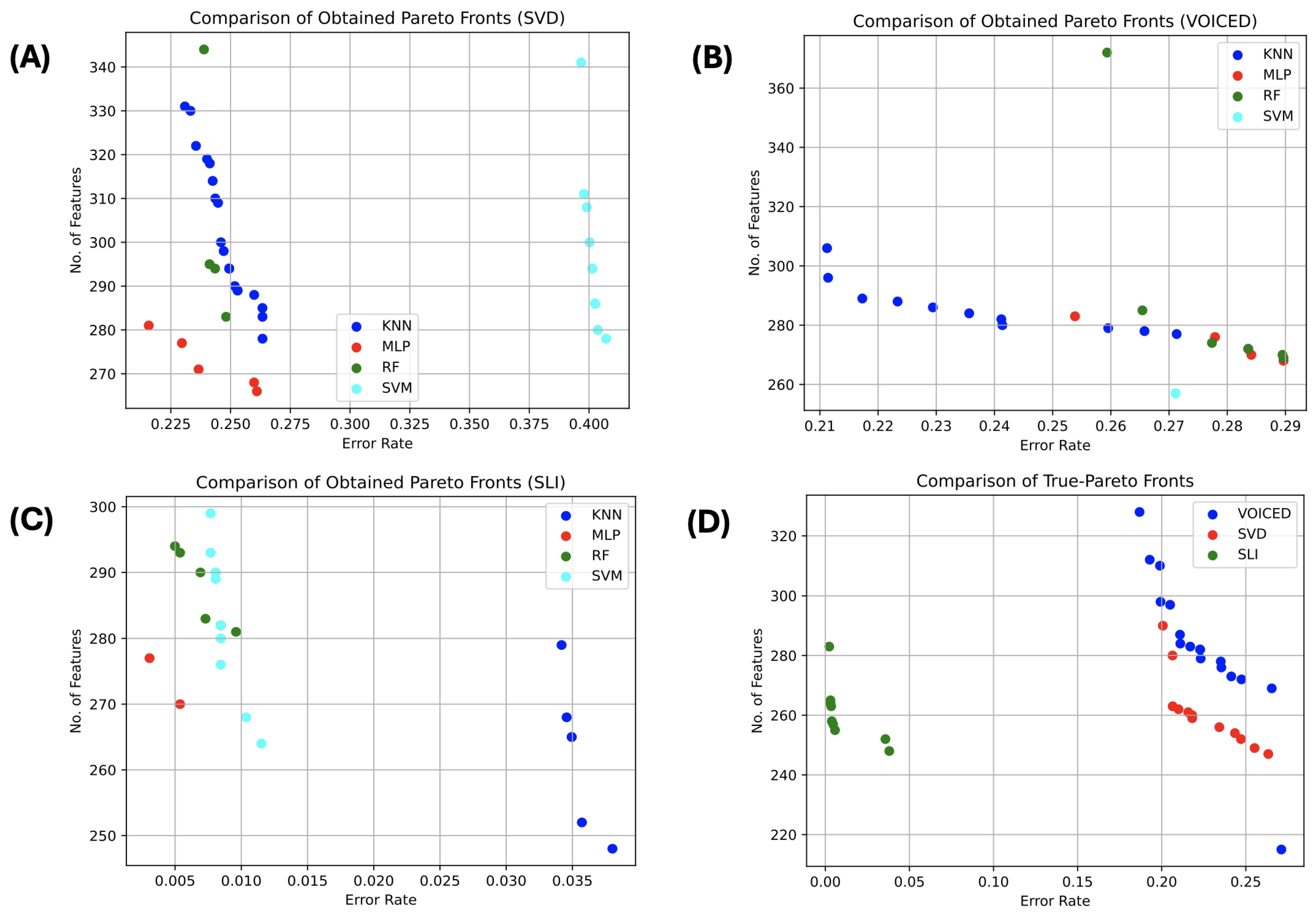
Figure 4 depicts the approximated Pareto-front for the three datasets from all optimizers and all classifiers. Figure 4A–C present the best obtained Pareto-front from the NSGA-II for SVD, VOICED, and SLI, respectively, among all classifiers. Figure 4D shows the actual Pareto-front (the non-dominated solutions) obtained by all classifiers over all runs.

Table 9. Optimization time of the NSGA-II over all classifiers and datasets.

Algorithm	Datasets	Optimization Time (s)
		AVG	STD
KNN	SLI	61.408	1.051
	SVD	20.021	0.266
	VOICED	8.319	0.947
MLP	SLI	7619.222	913.322
	SVD	3237.941	450.743
	VOICED	849.334	192.432
RF	SLI	7936.300	197.448
	SVD	4493.705	580.553
	VOICED	1045.188	65.990
SVM	SLI	834.729	25.778
	SVD	242.100	6.263
	VOICED	14.633	0.130

shows the required optimization time (i.e., training time) of the NSGA-II optimizer across KNN, MLP, RF, and SVM applied over the three datasets, with the average and standard deviation values computed. The optimization time represents the needed time for the optimization phase of the evolutionary algorithm to minimize the number of features and error rate. The results indicate significant variations in optimization time depending on the classifier and dataset. The MLP and RF classifiers are the most computationally intensive, particularly on the SLI dataset, with average times of 7619.2 s and 7936.3 s, respectively, which may reflect the higher complexity and resource demand of these models in training with NSGA-II. For smaller datasets like VOICED, all classifiers have lower optimization times, with KNN and SVM exhibiting particularly fast runtimes (8.319 s for KNN and 14.633 s for SVM). SVM shows consistently low optimization times across datasets, which may make it more practical for large-scale or real-time applications requiring NSGA-II optimization. The table highlights the computational demands of NSGA-II optimization, which vary substantially across classifiers and datasets, impacting its feasibility depending on the available resources and time constraints.

Furthermore, a statistical analysis is conducted to guarantee the significant difference in performance between the three evolutionary optimizers across the four machine learning algorithms and datasets. First, the Kolmogorov–Smirnov (KS) normality test is used to ensure the validity of the data distribution before computing the Analysis of Variance (ANOVA) test. If at least one dataset was abnormal, the Kruskal–Wallis test is calculated instead. The algorithms’ performance was evaluated using IGD and Hypervolume metrics over 15 independent runs. The test results exhibited a low p-value less than the significance level of 0.05, indicating a significant difference in the performance of the algorithms.

Generally speaking, NSGA-II is the best optimizer overall. While KNN performs best for SLI, MLP outperforms others in SVD, and SVM achieves the best IGD for VOICED, with MLP leading in HV, making NSGA-II and MLP a strong but not always the optimal solution. NSGA-II and MLP were used to compute the non-conformity scores for the three datasets. The split conformal prediction with softmax-based nonconformity scores is employed. Using the MAPIE Library [35], the CPs for all runs and all Pareto-fronts were computed, with the average (Avg.) and standard deviation (Std.) were reported for the non-conformity scores, as shown in

Table 10. Conformal predictions of NSGA-II and MLP.

Dataset	Accuracy	Nonconformity (Avg.)	Nonconformity (Std.)
SLI	0.987	0.015	0.079
SVD	0.743	0.253	0.364
VOICED	0.706	0.318	0.350

. The results show a strong performance of the SLI dataset with a high accuracy of 0.987 and low nonconformity scores (0.015 ± 0.079), indicating well-calibrated predictions and reliable uncertainty estimates. Conversely, the SVD and VOICED datasets exhibit lower accuracy (0.743 and 0.706, respectively) and higher nonconformity scores (0.253–0.318), suggesting increased model uncertainty or data challenges.

Table 11. Comparison of Proposed Method with State-of-the-Art Approaches.

Study	Method	Dataset	Accuracy	F1-Score	Precision	Recall
Junior et al. [15]	CNN + SMOTE	SVD	>90%	94.3%	-	-
Rehman et al. [16]	SVM + Feature Sel.	SVD, MEEI	99.97%	99%	-	-
Yadav et al. [18]	SL-RANN	SVD	94.35%	-	-	-
Albadr et al. [19]	FLN + MFCC	SVD	84.64%	86.80%	97.39%	86.05%
Yildirim et al. [21]	AOA + CNN + SVM	PD	96.62%	-	-	-
Akila et al. [23]	MASS-NN	PD (UCI)	99.1%	99.5%	-	-
Proposed Method	NSGA-II-based SVM	VOICED	69.0%	81.2%	71.8%	93.3%
Proposed Method	NSGA-II-based MLP	SVD	63.9%	66.7%	53.8%	87.6%
Proposed Method	NSGA-II-based KNN	SLI	81.3%	86.1%	85.5%	86.7%

presents a comparative overview of our proposed methods along with recent State-of-the-Art approaches from the literature. Although we acknowledge that the comparison is not strictly fair due to differences in datasets, feature extraction strategies, and optimization objectives, the table is intended to provide a contextual reference to understand current trends.

In particular, while many previous studies report high performance—particularly on the full SVD or mixed datasets (e.g., SVD + MEEI)—our experiments were conducted on different bases. Specifically, we used a subset of the SVD dataset, employed distinct handcrafted features (849 in total), and focused on underexplored datasets such as VOICED and SLI, for which, to the best of our knowledge, no multi-objective evolutionary optimization approaches have been previously applied.

The approach designed in this study emphasizes a multi-objective formulation using algorithms like NSGA-II to jointly minimize classification error and reduce the feature set. Despite relatively lower classification metrics in some cases, our methods achieve a threefold reduction in dimensionality, improving computational efficiency and interpretability.

Overall, although the table does not represent a direct benchmarking effort, it reinforces the unique value of this study’s contributions. Specifically, it emphasizes the integration of multi-objective optimization and the exploration of lesser-studied datasets. Thus, adding diversity and new directions to the existing body of research.

5. Conclusions

This comparative research study presents a new multi-objective and bio-inspired machine learning optimization approach for improving the accuracy of voice disorder detection. Three datasets were utilized along with three multi-objective optimizers (NSGA-II, SPEA-II, and MOEA/D) and four base classifiers (RF, KNN, MLP, and SVM). In this study, the problem is formulated as a multi-objective feature selection, which aims to minimize the number of features and the error rate. Several spectral and time-domain features were extracted from SLI, SVD, and VOICED datasets and labelled as normal and abnormal. Comparing algorithms based on the IGD, HV, Spread, and Spacing metrics showed that the three optimizers exhibited competitive performance, while the NSGA-II algorithm disclosed a powerful capability for identifying pathological voices. Also, the best classifiers per dataset are KNN for SLI (best IGD & HV), MLP for SVD (best IGD), and SVM for VOICED (best IGD), with MLP also excelling in HV. Although NSGA-II with MLP is not always the best, it remains a strong choice. Furthermore, by integrating conformal prediction, this study ensures statistically feasible uncertainty quantification in feature-selected models, enhancing the reliability of voice disorder detection even in high-dimensional settings.

Future research will investigate optimizing parameters and refining feature selection more closely, as these are important steps for promoting the performance of speech disorder detection. Incorporating advanced algorithms, such as deep neural networks, can further improve performance. Additionally, recent studies have shown the effectiveness of large language models (LLMs) in automatic speech recognition and speech analysis. Thus, this motivates the utilization of LLMs or speech large models for detecting and reconstructing corrupted speech. Nonetheless, a future work could refine conformal predictions by tackling calibration issues in lower-accuracy datasets (such as SVD and VOICED) or developing adaptive nonconformity scores to improve the precision of prediction sets.

References

1. Sapienza, C.; Ruddy, B. Voice Disorders; Plural: San Diego, CA, USA, 2009. [Google Scholar]
2. Abdulmajeed, N.Q.; Al-Khateeb, B.; Mohammed, M.A. A review on voice pathology: Taxonomy, diagnosis, medical procedures and detection techniques, open challenges, limitations, and recommendations for future directions. J. Intell. Syst. 2022, 31, 855–875. [Google Scholar] [CrossRef]
3. Guyon, I.; Elisseeff, A. An introduction to variable and feature selection. J. Mach. Learn. Res. 2003, 3, 1157–1182. [Google Scholar]
4. Yang, X.S. Metaheuristic optimization: Algorithm analysis and open problems. In Proceedings of the International Symposium on Experimental Algorithms, Chania, Greece, 5–7 May 2011; Springer: Berlin/Heidelberg, Germany, 2011; pp. 21–32. [Google Scholar]
5. Pham, T.H.; Raahemi, B. Bio-inspired feature selection algorithms with their applications: A systematic literature review. IEEE Access 2023, 11, 43733–43758. [Google Scholar] [CrossRef]
6. Deb, K.; Pratap, A.; Agarwal, S.; Meyarivan, T. A fast and elitist multiobjective genetic algorithm: NSGA-II. IEEE Trans. Evol. Comput. 2002, 6, 182–197. [Google Scholar] [CrossRef]
7. Zitzler, E.; Laumanns, M.; Thiele, L. SPEA2: Improving the Strength Pareto Evolutionary Algorithm; ETH Zurich: Zürich, Switzerland, 2001. [Google Scholar]
8. Zhang, Q.; Li, H. MOEA/D: A multiobjective evolutionary algorithm based on decomposition. IEEE Trans. Evol. Comput. 2007, 11, 712–731. [Google Scholar] [CrossRef]
9. Grill, P.; Tučková, J. Speech databases of typical children and children with SLI. PLoS ONE 2016, 11, e0150365. [Google Scholar] [CrossRef]
10. Woldert-Jokisz, B. Saarbruecken Voice Database. 2007. Available online: https://stimmdb.coli.uni-saarland.de/ (accessed on 5 May 2022).
11. Cesari, U.; De Pietro, G.; Marciano, E.; Niri, C.; Sannino, G.; Verde, L. A new database of healthy and pathological voices. Comput. Electr. Eng. 2018, 68, 310–321. [Google Scholar] [CrossRef]
12. Tirumala, S.S.; Shahamiri, S.R.; Garhwal, A.S.; Wang, R. Speaker identification features extraction methods: A systematic review. Expert Syst. Appl. 2017, 90, 250–271. [Google Scholar] [CrossRef]
13. Angelopoulos, A.N.; Bates, S. Conformal prediction: A gentle introduction. Found. Trends® Mach. Learn. 2023, 16, 494–591. [Google Scholar] [CrossRef]
14. Shafer, G.; Vovk, V. A tutorial on conformal prediction. J. Mach. Learn. Res. 2008, 9, 371–421. [Google Scholar]
15. Junior, S.B.; Guido, R.C.; Aguiar, G.J.; Santana, E.J.; Junior, M.L.P.; Patil, H.A. Multiple voice disorders in the same individual: Investigating handcrafted features, multi-label classification algorithms, and base-learners. Speech Commun. 2023, 152, 102952. [Google Scholar]
16. Rehman, M.U.; Shafique, A.; Jamal, S.S.; Gheraibia, Y.; Usman, A.B. Voice disorder detection using machine learning algorithms: An application in speech and language pathology. Eng. Appl. Artif. Intell. 2024, 133, 108047. [Google Scholar] [CrossRef]
17. Zhang, M.; Wang, Y.; Zhang, W.; Yang, M.; Luo, Z.; Li, G. Inductive conformal prediction for silent speech recognition. J. Neural Eng. 2020, 17, 066019. [Google Scholar] [CrossRef] [PubMed]
18. Yadav, K. Automatic detection of vocal cord disorders using machine learning method for healthcare system. Int. J. Syst. Assur. Eng. Manag. 2024, 15, 429–438. [Google Scholar] [CrossRef]
19. Albadr, M.A.A.; Ayob, M.; Tiun, S.; AL-Dhief, F.T.; Al-Daweri, M.S.; Homod, R.Z.; Abbas, A.H. Fast learning network algorithm for voice pathology detection and classification. Multimed. Tools Appl. 2025, 84, 18567–18598. [Google Scholar] [CrossRef]
20. Sindhu, I.; Sainin, M.S. Automatic Speech and Voice Disorder Detection using Deep Learning—A Systematic Literature Review. IEEE Access 2024, 12, 49667–49681. [Google Scholar] [CrossRef]
21. Yildirim, M.; Kiziloluk, S.; Aslan, S.; Sert, E. A new hybrid approach based on AOA, CNN and feature fusion that can automatically diagnose Parkinson’s disease from sound signals: PDD-AOA-CNN. Signal Image Video Process. 2024, 18, 1227–1240. [Google Scholar] [CrossRef]
22. Singh, N.; Sinha, S.; Singh, L. A novel WO-ANT: Whale-ant optimization algorithm for detection of Parkinson’s disease. Int. J. Inf. Technol. 2024, 17, 1873–1881. [Google Scholar] [CrossRef]
23. Akila, B.; Nayahi, J.J.V. Parkinson classification neural network with mass algorithm for processing speech signals. Neural Comput. Appl. 2024, 36, 10165–10181. [Google Scholar] [CrossRef]
24. Hadjaidji, E.; Amara Korba, M.C.; Khelil, K. Improving Detection of Parkinson’s Disease with Acoustic Feature Optimization Using Particle Swarm Optimization and Machine Learning. Mach. Learn. Sci. Technol. 2025, 6, 015026. [Google Scholar] [CrossRef]
25. Nasrolahzadeh, M.; Haddadnia, J.; Rahnamayan, S. Multi-objective optimization of wavelet-packet-based features in pathological diagnosis of alzheimer using spontaneous speech signals. IEEE Access 2020, 8, 112393–112406. [Google Scholar] [CrossRef]
26. Altay, E.V.; Alatas, B. Association analysis of Parkinson disease with vocal change characteristics using multi-objective metaheuristic optimization. Med. Hypotheses 2020, 141, 109722. [Google Scholar] [CrossRef] [PubMed]
27. Sheth, P.; Patil, S. Evolutionary Jaya Algorithm for Parkinson’s Disease Diagnosis using Multi-objective Feature Selection in Classification. In Proceedings of the 2019 5th International Conference On Computing, Communication, Control And Automation (ICCUBEA), Pune, India, 19–21 September 2019; IEEE: Piscataway, NJ, USA, 2019; pp. 1–4. [Google Scholar]
28. Patra, S.S.; Mittal, M.; Jena, O.P. Multiobjective evolutionary algorithm based on decomposition for feature selection in medical diagnosis. In Predictive Modeling in Biomedical Data Mining and Analysis; Elsevier: Amsterdam, The Netherlands, 2022; pp. 253–293. [Google Scholar]
29. McFee, B.; Raffel, C.; Liang, D.; Ellis, D.P.; McVicar, M.; Battenberg, E.; Nieto, O. librosa: Audio and music signal analysis in python. In Proceedings of the 14th Python in Science Conference, Austin, TX, USA, 6–12 July 2015; Volume 8, pp. 18–25. [Google Scholar]
30. Deb, K.; Kalyanmoy, D. Multi-Objective Optimization Using Evolutionary Algorithms; John Wiley & Sons, Inc.: New York, NY, USA, 2001. [Google Scholar]
31. Ishibuchi, H.; Masuda, H.; Tanigaki, Y.; Nojima, Y. Difficulties in specifying reference points to calculate the inverted generational distance for many-objective optimization problems. In Proceedings of the 2014 IEEE Symposium on Computational Intelligence in Multi-Criteria Decision-Making (MCDM), Orlando, FL, USA, 9–12 December 2014; IEEE: Piscataway, NJ, USA, 2014; pp. 170–177. [Google Scholar]
32. Biscani, F.; Izzo, D. A parallel global multiobjective framework for optimization: Pagmo. J. Open Source Softw. 2020, 5, 2338. [Google Scholar] [CrossRef]
33. Pedregosa, F.; Varoquaux, G.; Gramfort, A.; Michel, V.; Thirion, B.; Grisel, O.; Blondel, M.; Prettenhofer, P.; Weiss, R.; Dubourg, V.; et al. Scikit-learn: Machine learning in Python. J. Mach. Learn. Res. 2011, 12, 2825–2830. [Google Scholar]
34. Habib, M.; Vicente-Palacios, V.; García-Sánchez, P. Bio-inspired optimization of feature selection and SVM tuning for voice disorders detection. Knowl.-Based Syst. 2025, 310, 112950. [Google Scholar] [CrossRef]
35. Taquet, V.; Blot, V.; Morzadec, T.; Lacombe, L.; Brunel, N. MAPIE: An open-source library for distribution-free uncertainty quantification. arXiv 2022, arXiv:2207.12274. [Google Scholar]
Figure 1. A depiction of dominance, where both f 1 and f 2 are minimization functions. The grey points represent dominated solutions, while the blue dots indicate non-dominated solutions.
Algorithms 18 00338 g001
Figure 2. A representation of a solution, where the number of features is n, and i is the index.
Algorithms 18 00338 g002
Figure 3. Architectural design of the methodology.
Algorithms 18 00338 g003
Figure 4. Comparison of the best Pareto-Front per dataset and overall datasets.
Algorithms 18 00338 g004