Automatic Generation of Synthesisable Hardware Description Language Code of Multi-Sequence Detector Using Grammatical Evolution

Abstract

Quickly designing digital circuits that are both correct and efficient poses significant challenges. Electronics, especially those incorporating sequential logic circuits, are complex to design and test. While Electronic Design Automation (EDA) tools aid designers, they do not fully automate the creation of synthesisable circuits that can be directly translated into hardware. This paper introduces a system that employs Grammatical Evolution (GE) to automatically generate synthesisable Hardware Description Language (HDL) code for the Finite State Machine (FSM) of a Multi-Sequence Detector (MSD). This MSD differs significantly from prior work as it can detect multiple sequences in contrast to the single-sequence detectors discussed in existing literature. Sequence Detectors (SDs) are essential in circuits that detect sequences of specific events to produce timely alerts. The proposed MSD applies to a real-time vending machine scenario, enabling customer selections upon successful payment. However, this technique can evolve any MSD, such as a traffic light control system or a robot navigation system. We examine two parent selection techniques, Tournament Selection (TS) and Lexicase Selection (LS), demonstrating that LS performs better than TS, although both techniques successfully produce synthesisable hardware solutions. Both hand-crafted “Gold” and evolved circuits are synthesised using Generic Process Design Kit (GPDK) technologies at 45 nm, 90 nm, and 180 nm scales, demonstrating their efficacy.

1. Introduction

Designing digital circuits to meet specific requirements is a challenging task that demands significant effort from designers. This process is often time-consuming, and achieving an optimal design is not always guaranteed. To aid designers, EDA tools are used to enhance efficiency and produce more optimised circuits [1]. Some EDA tools incorporate Machine Learning (ML) techniques [2] or other forms of artificial intelligence [3,4] to assist in circuit design. However, current tools do not typically employ Evolutionary Algorithms (EA) to generate various circuit design solutions.

EAs are search-based techniques inspired by Darwinian evolutionary principles. They apply crossover and mutation, each with a set probability, to evolve toward an optimal solution for the given problem, mimicking natural selection to gradually enhance solution quality. The concept of genetic search was introduced by Alan Turing in 1948 [5]. Since then, the field of EAs has grown extensively, with applications in areas such as symbolic regression [6] and circuit design [7]. Prominent EA methodologies include Genetic Algorithms (GAs) [8], Genetic Programming (GP) [9], GE [10], and Evolutionary Strategies (ES) [11].

Evolvable Hardware (EH) refers to using EAs to evolve electronic circuits or their components. EH can be categorised into intrinsic and extrinsic evolution. Intrinsic evolution involves using hardware, such as Field Programmable Gate Arrays (FPGAs), to evolve and test solutions directly on the hardware in real time [12]. In contrast, extrinsic evolution relies on simulation tools to evolve and test circuits solely in a computer environment [13].

FPGAs are used to prototype digital circuits, which are specified at design time using HDLs, such as Very High-Speed Integrated Circuit HDL (VHSIC HDL or VHDL), Verilog, and SystemVerilog (SV), to describe circuit behaviour at different levels of abstraction. These languages enable designers to define circuits at both the gate level, using Boolean equations, and at the behavioural level, which is closer to high-level programming and includes constructs like loops and conditionals. The synthesis process then translates these descriptions into a gate-level netlist, which serves as the blueprint for physical implementation.

Digital sequential circuits, which differ from digital combinational circuits (detailed in Section 2) in their ability to store and manage state information, are critical in complex digital systems. These circuits are modelled using FSMs, which help represent the data flow and state transitions based on inputs. FSMs can be classified into two main types: Mealy machines and Moore machines (detailed in Section 2). In this work, we have evolved the MSD as a Mealy machine (shown in Figure 1) due to its ability to be highly responsive.

To the authors’ knowledge, no such MSD has been evolved in the literature using the evolutionary technique used in this work. As discussed in Section 4.1, GE is utilised to evolve this MSD and generate automatic HDL solutions. GE, a variant of GP that creates programs or expressions in virtually any syntax, uses context-free Backus–Naur Form (BNF) grammars for genotype-to-phenotype mapping. BNF is a formal notation used to describe the syntax of programming languages and data structures. It consists of production rules that define how non-terminal symbols can be expanded into sequences of terminal symbols and other non-terminals. More detail is given in Section 4.1.

These grammars allow the specification of rules that guide the evolution process. GE has been highly successful in various applications, including symbolic regression [14], classification [15], and particularly in automatic circuit design, whether combinational [16] or sequential [17], making it an ideal choice for this study. The decision to use behavioural-level HDL code instead of gate-level code for evolving this MSD is based on the recommendation for complex circuits [18] and its ability to evolve complex designs from the abstract level. Behavioural-level code is more straightforward to interpret [19] yet more challenging to evolve [20] due to its complex structures, such as if–else conditions and for loops.

MSDs are specialised sequential circuits that detect specific binary sequences, making them crucial in applications where sequence detection is critical, such as avionics and control systems. GE’s use in evolving these circuits allows for the automatic generation of HDL solutions, particularly at the behavioural level. Due to its complex structures, HDL code is easier to interpret but more challenging to evolve.

This study demonstrates the practical application of this approach through a case study involving a vending machine, which requires effective state management for tasks like product selection and payment processing. While the specific application in this paper is that of vending machines, the technique can be applied to any MSD, such as those commonly found in traffic light control systems [21], elevator control systems [22], robot navigation systems [23], and TCP/IP communication protocols [24].

By evolving the HDL code for a Mealy FSM-based Gold MSD, which acts as a benchmark circuit, the research compares different parent selection techniques and verifies the synthesisability of the evolved designs. A Mealy machine is a type of FSM where the output depends on both the current state and the current input (detail in Section 2). This work contributes to the field by exploring well-established methods for automatic circuit design in the context of evolving complex sequential circuits, such as MSD, using behavioural-level HDL.

The main contributions of this work are summarised as follows:

• We propose a GE-based approach to evolve SV code for solution circuits representing the FSM of a single-input, multi-output MSD, mapped to a real-life vending machine.
• We provide a theoretical analysis showing that prior work focuses only on single-input, single-output, single-sequence detectors, and no existing work addresses the evolution of FSMs of this complexity.
• We conduct extensive experiments demonstrating that GE combined with LS and TS can effectively generate solution circuits for such real-world problems. However, LS performs better than TS in terms of time and computational resources.
• Although GE, LS, and TS are well-established techniques, the novelty of this work is reflected by putting them all together to evolve the solution circuits of real-life complex FSMs.
• We show that the evolved solution circuits are synthesisable, and their synthesis reports outperform those of manually designed circuits.

The organisation of this paper is as follows: Section 2 gives a detailed background on all the technical aspects used. Section 3 provides a literature survey on the evolution of digital circuits. Section 4 introduces GE and details the parent selection techniques employed in this study. Section 5 describes the process of generating training and test datasets necessary for the proposed work. Section 6 presents the experiments and results. Section 7 shows one of the perfectly evolved FSMs and compares it with a human-made FSM. Section 8 shows and compares the synthesis of the Gold and evolved solutions, highlighting the performance differences between human-designed and machine-generated solutions. Finally, Section 9 concludes the paper and discusses future directions in this field of research.

2. Background

HDLs are programming languages that describe digital circuits at the gate or behavioural (algorithmic) level. In gate-level descriptions, the circuit’s architecture is defined using Boolean equations. In contrast, at the behavioural level, circuits are described using a high-level language similar to C, which includes constructs such as loops and if–else conditionals. Since we are working on the evolution of an FSM, no loops are used in this work, only conditionals, as the loops have no use here. Describing a circuit at the behavioural level significantly reduces the programmer’s effort. The most widely used HDL standards are VHDL [25] and Verilog HDL [26]. SV [27], employed in this work to design and evolve sequential circuits, is an extension of Verilog HDL that enhances verification capabilities, earning it the designation of Hardware Verification Language (HVL) and an HDL.

Once a circuit’s design is complete and its logical correctness verified through simulation, the next phase is logic synthesis. This process converts the HDL code into a netlist, which defines the circuit at the gate level using Boolean equations or registers. The netlist acts as a blueprint for constructing the circuit’s logical structure. Tools like Cadence Genus [28] are used to optimise the synthesised design to meet specific criteria, including area, power consumption, system delay, and overall performance, based on predefined specifications such as operating temperature and transistor sizes targeting particular fabrication technologies.

However, even if a circuit passes simulation, physically constructing the chip might not be possible. This can occur if the netlist cannot be generated, often due to combining synthesisable and non-synthesisable constructs. For instance, loops in hardware must have known boundaries at compile time, even though they do not need them at simulation time. When loops have variable or non-static bounds, they cannot be synthesised. If we take the example of a for loop, the code will not be synthesised if the value of N is not known in for (i = 0; i < N; i = i + 1) at the synthesis time.

Digital circuits are broadly classified into two types: combinational circuits and sequential circuits. Combinational circuits produce outputs solely based on the current inputs, without memory of past inputs. In contrast, sequential circuits include memory elements that store information about the system’s current state, making the output dependent on both the current state and the current input. Examples of basic sequential circuits include the JK Flip-Flop and the Up–Down Counter. Sequential circuits can be effectively modelled using FSMs. Because the output of a sequential circuit depends on its current state, FSMs are powerful tools for representing the data flow in terms of state transitions based on the inputs and the system’s current state [29].

There are two primary types of FSMs: Mealy machines and Moore machines. In both types, the next state is determined by the system’s current state and the circuit input. However, the critical difference lies in how the output is generated. In a Mealy machine, the output depends on the current state and input. In contrast, in a Moore machine, the output depends only on the current state. In this work, we are evolving the circuit based on Mealy FSM shown in Figure 1. We use Mealy machines because they respond quickly and typically require one state fewer than Moore machines, saving both time and hardware resources. However, Mealy machines can propagate transient input glitches—short, unintended signal fluctuations in a digital circuit—directly to the output if present. This is a trade-off we accept to achieve a high-speed and efficient system.

SDs vary in complexity depending on their size and features. As the name suggests, SDs detect specific binary sequences, such as ‘110011’, and produce the desired output upon successful detection. They play crucial roles in real-time critical systems, such as avionics, where detecting a series of events in the correct order is essential. These systems must be highly responsive, meticulously designed, and thoroughly tested under all possible conditions to ensure they do not fail to generate necessary alarms.

This work proposes evolving behavioural-level HDL code using GE for a single-input, multi-output MSD. MSD is crucial in designing complex systems that require multiple states and transitions based on varying inputs. They are used in various applications where state management is critical, such as digital systems, embedded systems, and communication protocols. Speaking of their real-world applications, MSDs are fundamental in designing control systems for machinery, robotics, and other automated processes. Their ability to manage multiple states and transitions makes them suitable for real-time systems where efficient state management is crucial.

We apply this work to a real-life vending machine scenario, which provides a concrete example of how MSDs can be applied in real-world systems. Vending machines involve state management for product selection, payment processing, and item dispensing, making them an ideal test case for MSD designs. Moreover, the vending machine example highlights the complexity involved in real-world applications. It shows how MSDs can handle various states and transitions required to process inputs and provide outputs, demonstrating the practical value of evolving synthesisable HDL codes for such systems.

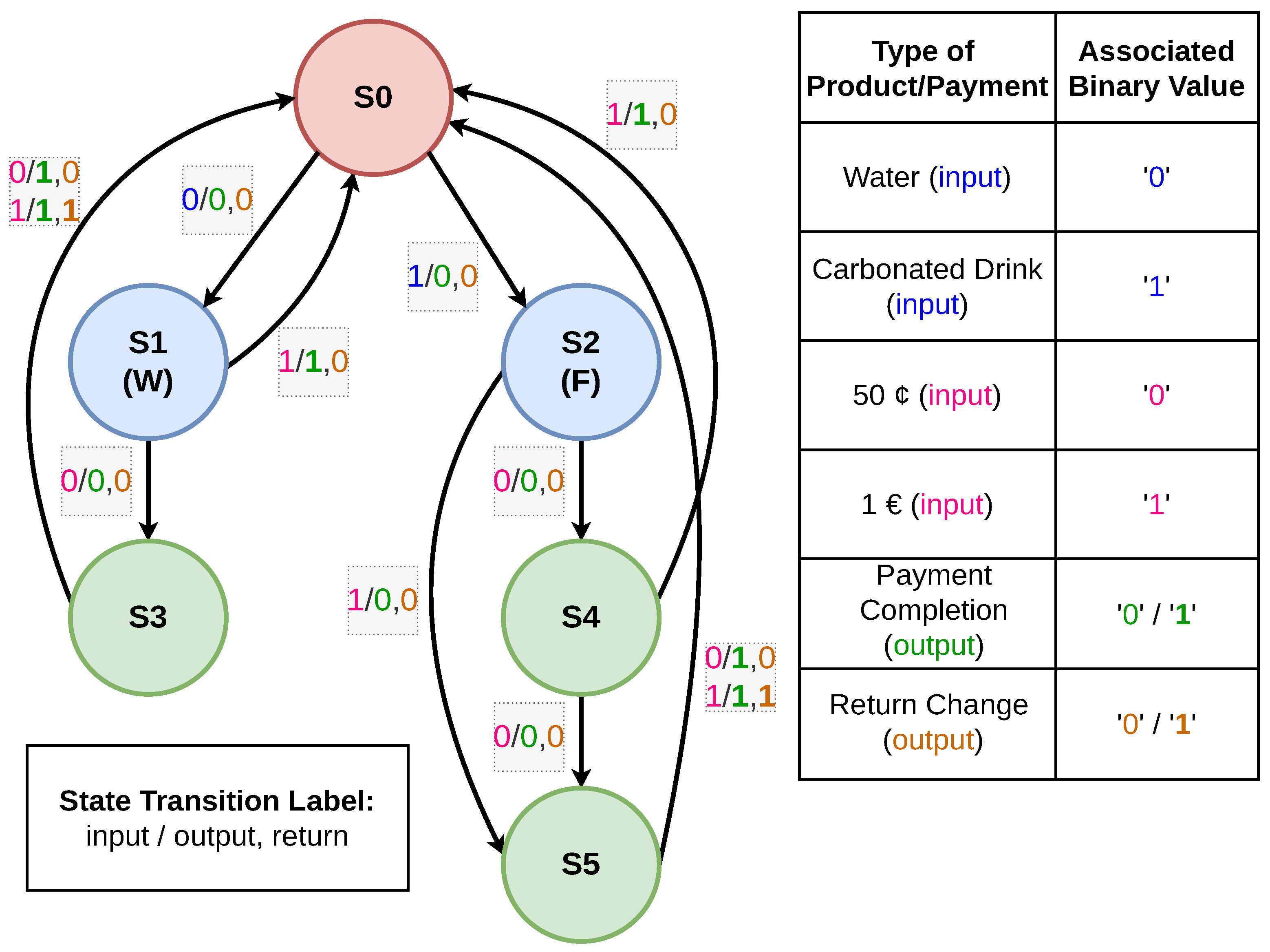
The Mealy FSM for the Gold MSD, representing a human-designed target circuit, is shown in Figure 1. “Gold” refers to the benchmark circuit the evolutionary system aims to achieve. This MSD can identify two distinct sequences, process a single 1-bit input, and produce two 1-bit outputs each clock cycle. The system starts at state S0 after a reset or upon waking from its idle state. The customer can choose between water and a carbonated drink. If the customer selects water (binary input ‘0’), the machine transitions to state S1 (labelled ‘W’). Conversely, if the carbonated drink is selected (binary input ‘1’), the system moves to state S2 (labelled ‘F’). After this selection, the system waits for payment. If the payment is incomplete within a specified time, the product is not dispensed, and the system resets to S0. We are assuming that the water costs EUR 1, while the carbonated drink costs EUR 1.50, with the system accepting only EUR 0.50 (binary input ‘0’) and EUR 1 (binary input ‘1’) coins.

In state S1, if the system receives EUR 1, it returns to S0, and the first output (leftmost) turns ‘1’, indicating full payment and dispensing the water. However, if only EUR 0.50 is received, the system transitions to S3, keeping both outputs at ‘0’ to indicate that additional payment is required. If another EUR 0.50 is received at S3, the system returns to S0, setting the first output to ‘1’ to confirm full payment. If EUR 1 is received at S3, the system resets to S0 but also sets the rightmost output to ‘1’, indicating that EUR 0.50 must be returned to the customer. For S2, the system transitions through states S4 and S5, eventually returning to S0 if three consecutive EUR 0.50 coins are inserted. If a EUR 1 coin is inserted at any point, the system bypasses certain states and returns to S0, providing appropriate outputs for payment processing and correct change. Note that in any given transaction, the maximum return possible is EUR 0.50.

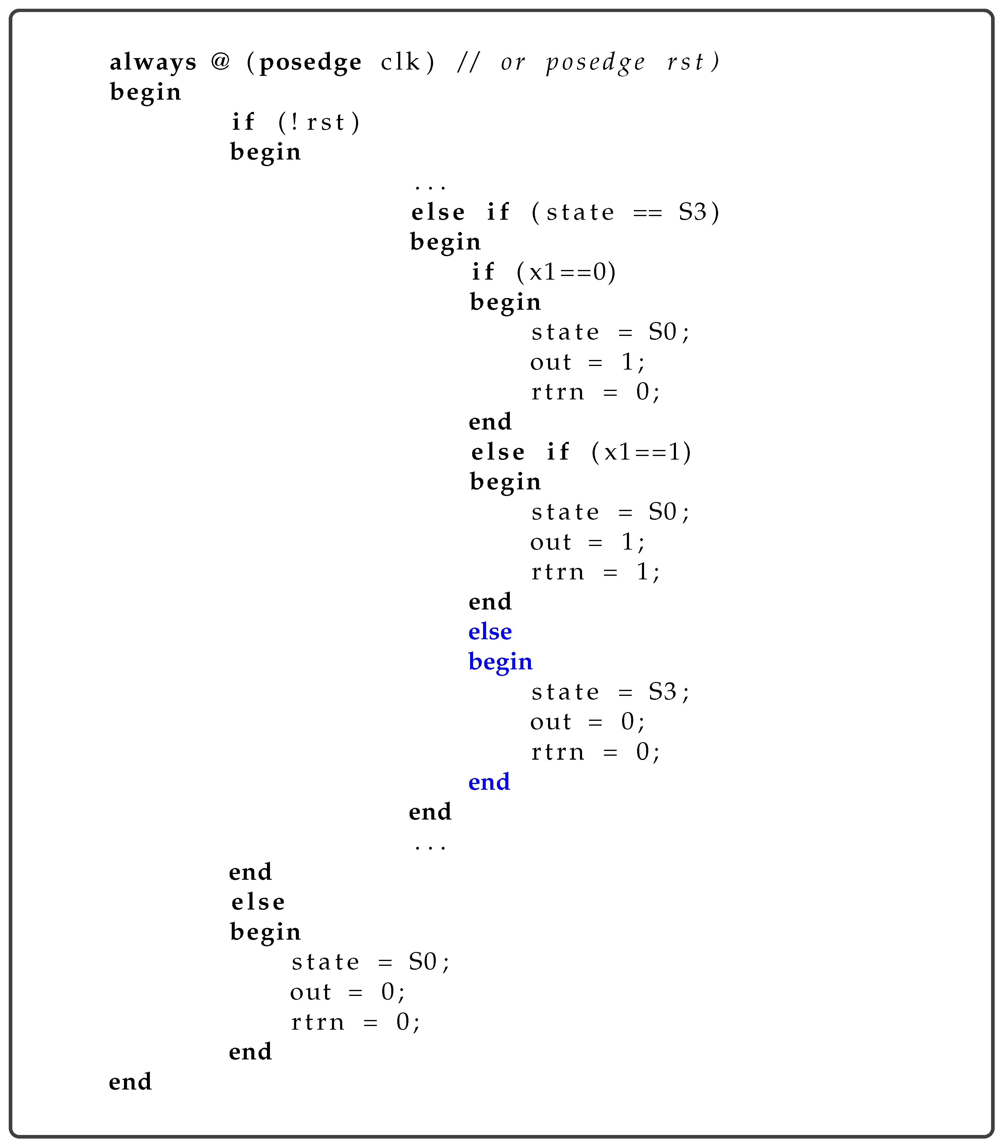
As discussed above and shown in Figure 1, from any stage, there are two possible transitions: one dependent on input ‘1’ and the other on input ‘0’. If, at any stage, the system does not receive any input—neither ‘1’ nor ‘0’—it remains in the same state and outputs ‘0’ for both product delivery and return change. An example of such a transition in the SV code of the human-designed FSM is shown in Figure 2 (full code given in Supplementary Material (SM), https://github.com/bmmajeed/MSD_VendingMachine (accessed on 2 June 2025), where the section’s condition over the code responsible for this behaviour is highlighted in blue. These transitions are not explicitly shown in Figure 1 to prevent the diagram from becoming overly complex. However, in Section 7, it will be shown how these transitions affect the system’s output, as the assignments within this else block are subject to evolution. Although the structure of the FSM is hardcoded, the system retains full flexibility to evolve all the assignments in the code.

3. Related Work

The origins of EH can be traced back to 1985 when Fourman et al. used GA to create compact symbolic circuit layouts [30], although the term “EH” was not used then. Subsequent studies, such as those by Cohoon et al. [31] and Kling et al. [32], employed GAs to optimally place components on circuit boards. In 1992, Koza [9] pioneered the use of GP to develop complete circuits at the gate level. This involved a decomposition method where an 11-to-1 multiplexer was evolved using two 6-to-1 multiplexers, which evolved from 3-to-1 multiplexers. The term “EH” was first introduced by [33] in 1993, marking a significant step towards the practical implementation of the “Darwin Machine” [34], where combinational circuits were evolved.

Considerable research has been conducted on the evolution of combinational circuits using various methods, including ES [35], Cartesian Genetic Programming (CGP) [36], and GE [16,37,38]. While significant work has been conducted on the evolution of FSMs or Deterministic Finite Automata (DFAs) [39,40,41,42], there has been less research on evolving sequential circuits, explicitly from the perspective of FSMs [43,44,45,46]. Notable examples include [47] and [17], where single-input, single-output SDs were evolved.

Ali et al. presented the first automatic solution for gate-level SD evolution using GA in 2004 [48]. They evolved a 4-bit SD (‘1010’) and a 6-bit SD (‘011011’) through a multi-stage evolutionary process, which was resource-intensive and did not directly produce the final solutions. The 6-bit SD combined two 3-bit SDs (‘011’). The same circuits were re-evolved using GA, achieving more optimised solutions with reduced computational cost [49].

In 2007, Yao et al. evolved a 3-bit SD (‘110’) using an incremental, evolutionary approach based on GA [50]. This approach involved developing basic module circuits via a greedy search to construct more extensive, complex circuits. However, the approach needed to be expanded in scope, targeting specific modules and thus limiting the search space, preventing the generation of generalised solution circuits. In 2009, Xiong et al. evolved an overlapping 3-bit SD capable of detecting sequences like ‘101’ and ‘100’, utilizing intrinsic evolution on an FPGA board [51]. They later demonstrated this system’s real-life application in a cardiovascular system [52], evolving the same SD using intrinsic and extrinsic evolution methods based on GA, showcasing the system on an FPGA board. Both approaches were computationally expensive for a small 3-bit SD.

In 2011, Soleimani et al. [47] revisited the evolution of the circuits initially evolved by Ali et al. [48] and Popa et al. [49] using a GA. They claimed to have used fewer gates than the earlier work by Ali et al., although they did not compare their results with Popa’s work.

Tao et al. in 2012 evolved a 4-bit SD using GA and GP [53]. This incremental evolution process involved evolving basic circuits as modules before developing complex circuits from these modules. Using three evolutionary stages for a relatively simple 4-bit SD underscored the high computational cost.

Previous research has primarily focused on the gate-level evolution of SDs using GA and GP. The first work on behavioural-level SD evolution was presented in [17], where 3, 4, 5, and 6-bit SDs were evolved using GE. This work successfully evolved behavioural-level HDL codes from the perspective of FSMs, with the 3, 4, and 5-bit SDs being evolved in a single evolutionary stage. However, due to its complexity, the 6-bit SD required a second evolutionary phase incorporating grammar encapsulation. In this phase, the grammar is provided with the best individual achieved so far, allowing the system to evolve further from that point (detail in the [17]).

Building on this, we presented an improved performance in [44], where the same circuits were evolved using LS and a minimal set of test cases for training. This approach improved the performance of all circuits and enabled the evolution of the 6-bit SD in a single stage.

However, the studies above have focused exclusively on developing SDs for single-sequence detection; research has yet to explore the evolution of SDs capable of detecting multiple sequences. Additionally, while extensive research has been conducted on designing FSMs for vending machines [54,55,56,57], the evolutionary development of a vending machine-like FSM has not been investigated.

The evolutionary development of a vending machine-like FSM is a significant contribution and demonstrates the potential for automating the design of complex, real-world systems. This research demonstrates the capability of automating and optimising state management in digital systems by evolving FSMs for scenarios such as vending machines involving multiple states and decision points. This approach bridges theoretical methods with practical applications and paves the way for more efficient and innovative designs in various automated systems and consumer devices.

4. Evolutionary Computation Technique and Parent Selection Methods

4.1. Grammatical Evolution

GE [10] is a variation of GP that uses GAs to evolve variable-length binary strings, known as genotypes. These genotypes are mapped to programs or structures, referred to as phenotypes, in any language defined by a BNF grammar. This capability allows GE to evolve constructs in various programming languages.

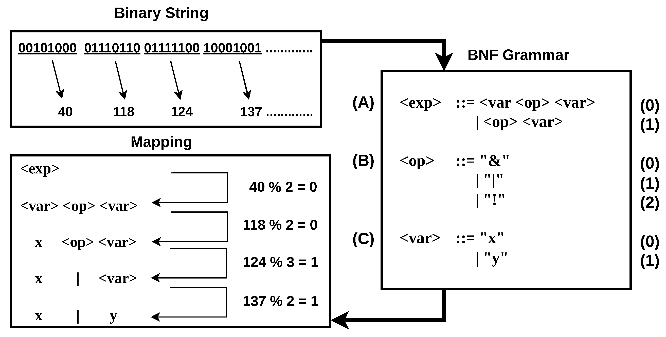
BNF is a notation used to describe context-free grammars. Figure 3 illustrates the GE mapping process in detail. BNF grammars consist of four key components:

1.

Production Rules (P): These define how a non-terminal symbol can be replaced with a combination of other symbols (terminals or non-terminals), guiding the generation of valid strings in the language defined by the grammar.

2.

Terminals (T): These are the items that can appear in the final program and, in context-free grammars such as those used in this work, only on the Right-Hand Side (RHS) of a production rule and cannot be further expanded. Examples include symbols like ‘!’ and ‘&’ in the given grammar.

3.

Non-Terminals (N): These are intermediate elements that are mapped by the production rules into members of the set T; these elements can appear on both the Left-Hand Side (LHS) and RHS of production rules and can be expanded into other non-terminals or terminals. For instance, $<\mathrm{var}>$ is a non-terminal in the example.

4.

Start Symbol (S): This is a special non-terminal from which the derivation begins. It appears in the first production rule and is typically the leftmost non-terminal, such as $<\mathrm{expr}>$ in the first production rule shown in Figure 3.

The genotype, a binary string, is divided into codons and then converted into decimal integers. In the example shown in Figure 3, 8-bit codons of the genotype are used for this conversion. The first integer obtained is 40. The mapping process begins with the S from the first production rule (A). Given two possible RHS options in this rule, the selection is made using the modulus operation: the integer 40 modulo 2 equals 0, thus selecting the first option.

Next, the selected option contains a non-terminal, expanding the leftmost non-terminal. The second integer, 118, determines the selection within the non-terminal $<\mathrm{var}>$, which has two options according to the third production rule (C). The operation 118 modulo 2 equals 0, so the first option, the variable ‘x’, is chosen. The subsequent non-terminal $<\mathrm{op}>$ has three options according to the second production rule (B). Using the third integer, 124, the selection is made by calculating 124 modulo 3, resulting in 1, thus choosing the second terminal, representing an OR operation. Finally, for the last non-terminal $<\mathrm{var}>$, the integer 137 modulo 2 results in 1, selecting the variable ‘y’. The resulting expression, shown in Figure 3, is an OR operation between the inputs ‘x’ and ‘y’. This example is adapted from [17], where a more detailed explanation can be found.

4.2. Tournament vs. Lexicase Parent Selection

The parent selection method plays a critical role in the evolutionary process. In TS [58], a tournament is conducted among n individuals. The one with the best overall performance across all training cases, i.e., the highest aggregated fitness value, is selected. In this study, the value of n is set to 2 for all experiments to save computational time and cost. While this smaller tournament size increases the chances of low-fitness candidates being selected as parents and high-fitness candidates being missed [58], this effect is mitigated in our case due to the significant population sizes used. Larger populations increase diversity and the likelihood of high-fitness candidates being retained, ensuring robust evolutionary progress despite lower selection pressure.

In contrast, LS [59] does not rely on an aggregated fitness value. Instead, it selects specialists who excel at particular training cases. The process begins by considering the entire population, with individuals filtered out iteratively based on their performance on random training cases. The individual who performs best on the selected training case is chosen as a parent. One is randomly selected if two or more individuals perform equally well on a training case. LS has demonstrated exceptional problem-solving abilities in various fields, including regression [60] and evolutionary robotics [61]. Notably, it has shown outstanding results in the evolution of both combinational [20,37,38] and sequential [44] digital circuits in recent years.

5. Dataset Generation

The choice of training dataset is crucial in developing sequential circuits. The dataset can be random, exhaustive (where the system is initialised to a specific state and evaluated against all possible inputs), or selectively chosen based on the designer’s preferences. The size or length of each training case within the dataset also plays a significant role.

In the FSM mapped to a vending machine, the number of training or test cases is limited, with each case having a specific length (the details are given below). The dataset shown in Figure 4, as shown below, includes all required training cases. In addition to having all the necessary training cases, it also represents the complete set of possible test cases for this FSM, as there are no additional scenarios applicable to this FSM. If the number of train and test cases is changed from those used in this work, it will increase the search space tremendously, and the trade-off would be a drastic decrease in success rate under a given setting of hyperparameters, which is not a useful trade-off. Since the training and test cases are the same, in Figure 4 they are indicated as TC. This contrasts with the more extensive test datasets used for testing other evolved SDs, such as those in [44,48]. If the train and test cases are kept different from each other and we have an unbalanced dataset, we can use a cluster-based approach, such as a hamming distance-based approach, to balance the dataset.

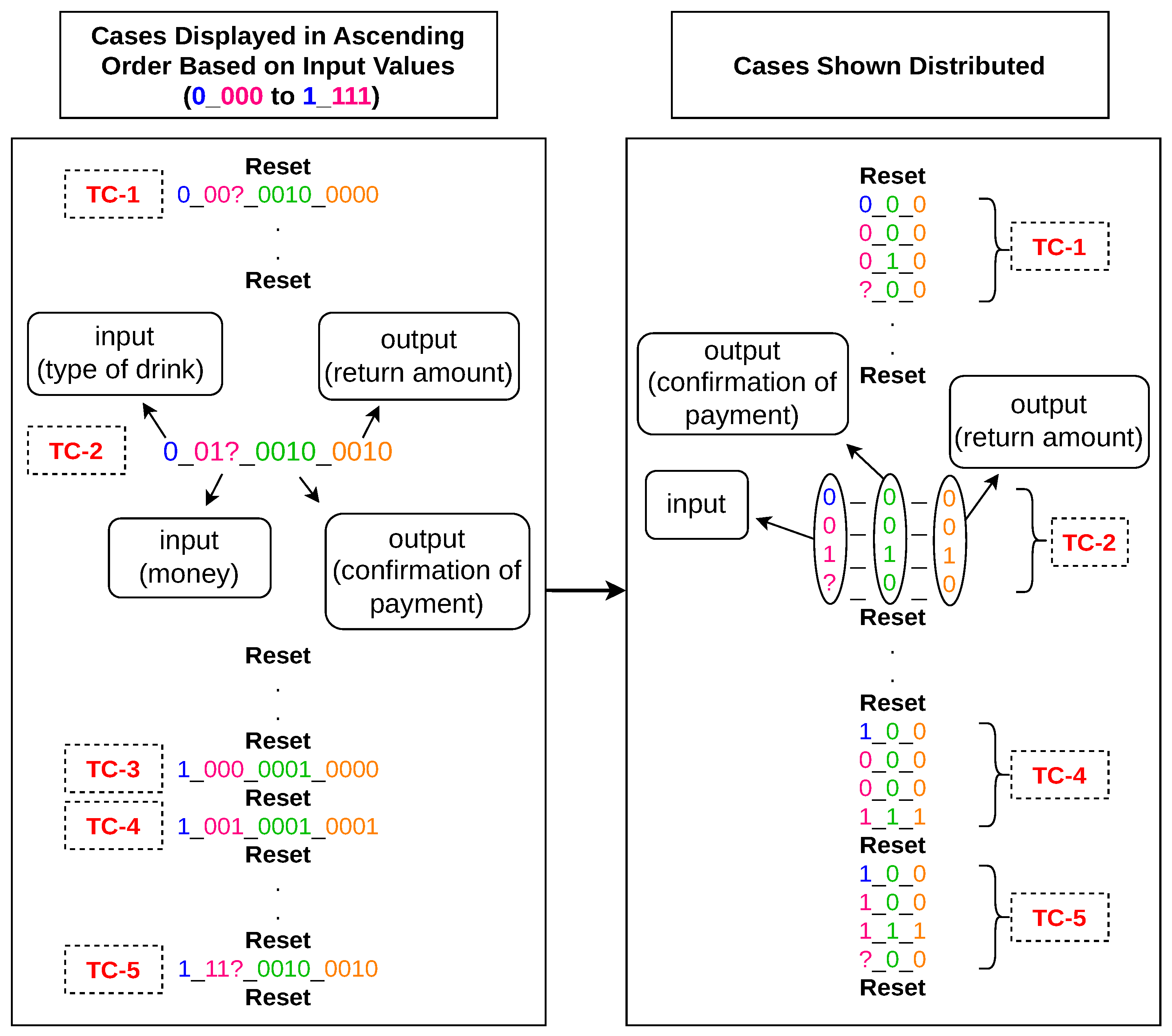
The TCs are presented in two formats for ease of explanation, as illustrated in Figure 4. On the left, the TCs are displayed input-wise, from ‘0_000’ to ‘1_111’, for clarity and ease of understanding. There are five example TCs shown in this figure, and they are selected as of mixed complexity to demonstrate the FSM’s ability to handle both simple and extended input-output sequences involving varying payment paths and change-return scenarios. Take the example of the TC-2 ‘0_01?_0010_0010’. The higher order four bits (in this TC, ‘0_01?’) represent inputs in product selection and payment status. The most significant bit indicates whether the customer selects water (‘0’) or a carbonated drink (‘1’). The following three input bits immediately after the underscore (‘_’) represent what payment has been made for the selected product. As mentioned above, the water costs EUR 1, while a carbonated drink costs EUR 1.50. Therefore, these four bits indicate that the customer selected water, indicated by input ‘0’, and then paid EUR 0.50 and EUR 1, indicated by ‘0’ and ‘1’, respectively. At this point, the payment is completed, and now the customer needs to be served with water and a return of EUR 0.50. In this scenario, the fourth bit in the input sequence of ‘0_01?’ is taken as a don’t care bit, shown as ‘?’, and is neglected since the third input bit completes the payment. ‘?’ indicates that the bit can be a ‘0’, ‘1’, or ‘x’ (no input at all) in this clock cycle. The same happens in TC-5, where the fourth bit in the input sequence is also neglected, but it does not always happen. It can be seen in TC-3 and TC-4 that after the fizzy drink (‘1’) is selected at the first bit of the input sequence, the payment is not completed by the end of the third bit in the input sequence, so the fourth bit is adding the value to the payment required to get the product delivered. Please refer to Figure 1 to understand this step in more detail.

The next two 4-bit chunks (‘0010_0010’ in TC-2), from left to right, in the training and test vectors, also separated by an underscore (‘_’), represent the system’s outputs: first confirming payment and the other returning any necessary change. The outputs are determined by combining the inputs and the system’s state, as depicted in Figure 1 and discussed in Section 2. For input sequence TC-2 ‘0_01?’, the first output sequence, ‘0010’, with ‘1’ at the third bit from left to right, reflects that the drink is served in the third cycle when the payment of EUR 1.50 is completed. This is because the consumer consumed the first two cycles, selecting the product and adding coins. Hence, the output is ‘0’ in those two cycles. Since the payment of EUR 1.50 is more than the price of water, which is EUR 1, the ‘1’ at the third bit from left to right in the following output sequence ‘0010’ tells that in the third cycle, the customer has been paid with a change of EUR 0.50 along with the product.

The vending machine can only ever issue EUR 0.50 change. In this instance, EUR 0.50 was issued, and it happened in the same cycle as the drink being delivered. The change will always be issued in the same cycle as the delivered drink in the proposed system. Similarly, if there is no change, the final four bits will always be all zeroes. Since in the discussed TC here, the fourth bit in the input sequence is a don’t-care bit, the outputs stay the same for the TCs with input sequences of ‘0_010’, ‘0_011’, or ‘0_01x’.

Note that we assume that the customer can only use EUR 0.50 and EUR 1 coins and that the vending machine will accept a specific amount of these coins in each cycle. Other coins are ignored.

On the right side of the dataset shown in Figure 4, each 12-bit TC from the left side is broken into four 3-bit vectors. Each vector has three bits, separated by ‘_’, where the first bit indicates the input, and the remaining two bits represent the relevant outputs of the system for that input.

For example, the four input bits ‘0_011’ from TC-2 on the left side are reflected in the leftmost bit of the four distributed vectors on the right side. Similarly, the four bits ‘0010’ shown in the middle of TC-2 on the left side of Figure 4 are represented in the middle bit of the vectors on the right side of the figure. Finally, the four bits ‘0010’ from the rightmost part of TC-2 on the left side are reflected in the rightmost bit of the distributed vectors on the right side. These three sections of the distributed vectors of TC-2 are enclosed in ovals and are properly labelled as shown on the right side of Figure 4 for a better understanding.

In this defined way, the TCs are distributed and fed into the system during each cycle, determining the system’s fitness value against each TC. There are 16 12-bit TCs on the left side, which, when distributed according to the system’s requirements, result in 64 3-bit vectors on the right side, which are fed into the system in each cycle. Thus, the maximum fitness value is 64. The maximum fitness value for an individual is only achieved if the individual correctly resolves all the TCs.

The pseudocode to generate the train/test dataset for a complex FSM, such as the one presented here, is shown in Algorithm 1. The process begins by initialising the FSM configuration, such as the vending machine logic discussed earlier. The input encoding is defined such that the first bit represents the product selection (with ‘0’ for water and ‘1’ for a fizzy drink), while the next three bits represent the payment sequence, where ‘0’ and ‘1’ correspond to EUR 0.50 and EUR 1 coins, respectively, and ‘?’ denotes a don’t-care condition. The output encoding is similarly defined, where the first four bits represent the delivery signal across clock cycles, and the next four bits represent the issuance of a return change if applicable. An empty dataset list is then initialised, and for each valid product and payment scenario, an input sequence is generated. The FSM transitions are simulated cycle-by-cycle to compute the corresponding delivery and return change outputs based on the system’s logic and state evolution. Each TC is formatted by concatenating the input sequence, delivery output, and return change output into a 12-bit vector and is subsequently added to the dataset.

Algorithm 1 Generate Training Dataset for FSM Evolution.

1: function  GenerateDataset 2:     Initialise FSM configuration             // e.g., vending machine logic 3:     Define input encoding: 4:         1st bit: product selection                 // 0 = water, 1 = fizzy drink 5:         Next 3 bits: payment sequence     // 0 = €0.50, 1 = €1, ? = don’t care 6:     Define output encoding: 7:         4 bits: delivery signal per cycle 8:         4 bits: return change signal per cycle 9:     Initialise empty dataset list D 10:   for all valid product and payment scenarios do 11:         Generate input sequence I                                 // 4 bits 12:         Simulate FSM state transitions for each cycle 13:         Compute outputs: 14:             Product delivery signal based on when payment completes 15:             Return change signal if overpayment occurs 16:         Format test case: $TC=I·O_{delivery}·O_{change}$ 17:         Add $TC$ to dataset D 18:     end for 19:     Initialise empty evaluation list V 20:     for all $TC$ in D do 21:         Split $TC$ (12 bits) into four 3-bit vectors: 22:         for $i=1$ to 4 do 23:            $v_i\leftarrow (input\left[i\right],delivery\left[i\right],change\left[i\right])$ 24:            Add $v_i$ to V 25:         end for 26:     end for 27:     return V                // 3-bit vectors for GE fitness evaluation 28: end function

In the distribution step tailored for the system’s evaluation, each 12-bit TC is further split into four smaller vectors, each consisting of three bits. Each 3-bit vector comprises a single input bit and two associated output bits, corresponding to the delivery and return change signals for that particular cycle. These distributed vectors are then collectively used for fitness evaluation during the evolutionary process. The correct resolution of all vectors is essential for an individual to achieve the maximum fitness score. This structured approach ensures that all possible TCs relevant to the FSM are covered comprehensively, facilitating effective learning and circuit evolution within the GE framework.

While the dataset size is deliberately constrained to ensure complete coverage with minimal redundancy, the test complexity arises from the sequencing of state-specific inputs and strict timing constraints enforced by the FSM structure. Future work may explore extensional models, such as those proposed by Rodríguez et al. [62], to formally assess and adapt test complexity in broader, adaptive scenarios.

6. Experiments and Results

6.1. Experimental Setup, Tools, and Evolutionary Parameters

All experiments for this work were conducted using a setup that integrates Icarus Verilog (a Verilog/SV simulator) with Grammatical Algorithms in Python for Evolution (GRAPE) [63], a Python-based implementation of GE. The solutions evolved in GRAPE and were evaluated for each generation using Icarus Verilog to calculate the fitness value. The experiments were performed on a Dell OptiPlex 5070 (sourced from Dell Technologies Customer Solution Center, Limerick, Ireland) desktop computer with a 1 TB HDD, 256 GB SSD, a single 16 GB RAM module, and a 64-bit quad-core 9th-generation i7 processor with a 12 MB cache. The processor’s standard operating frequency is 3.0 GHz, which can boost up to 4.7 GHz in turbo mode. The system uses the operating system Ubuntu 22.04.4 LTS.

The hyperparameters used in this work are detailed in

Table 1. Hyperparameters used for experiments.

Hyperparameter	Value
No. of Runs	30
Population Size	1000
No. of Gens.	30
Initialisation	Sensible
Mutation Prob.	0.01
Crossover Prob.	0.9
Elitism	Yes
Training Cases	64
Test Cases	64

. All experiments initially used a population of 1000 and ran for 30 generations. However, these parameters were increased for some experiments, with results presented according to the respective population size and maximum number of generations in

Table 2. Success rate and execution time of evolved SDs according to the LS and TS method with respective population size and number of generations. (NN stands for “Not Needed” and is used where a success rate of 25/30 or more is achieved and needs no more experiments. These success rates mark the successful runs and are highlighted in green. Unsuccessful runs are shown in blue).

Parameter Values		Training and Test Results Using LS		Training and Test Results Using TS
Population Size	Number of Generations	Success Rate	Execution Time	Success Rate	Execution Time
1000	30	09/30	57 min 42 s	02/30	59 min 36 s
	100	17/30	178 min 41 s	06/30	177 min 42 s
	500	29/30	867 min 56 s	20/30	870 min 23 s
	1000	NN	NN	23/30	1732 min 53 s
5000	100	NN	NN	20/30	872 min 45 s
	500	NN	NN	30/30	4348 min 15 s

. The experimental setup is designed to run 12 runs in parallel on 12 threads of the processor.

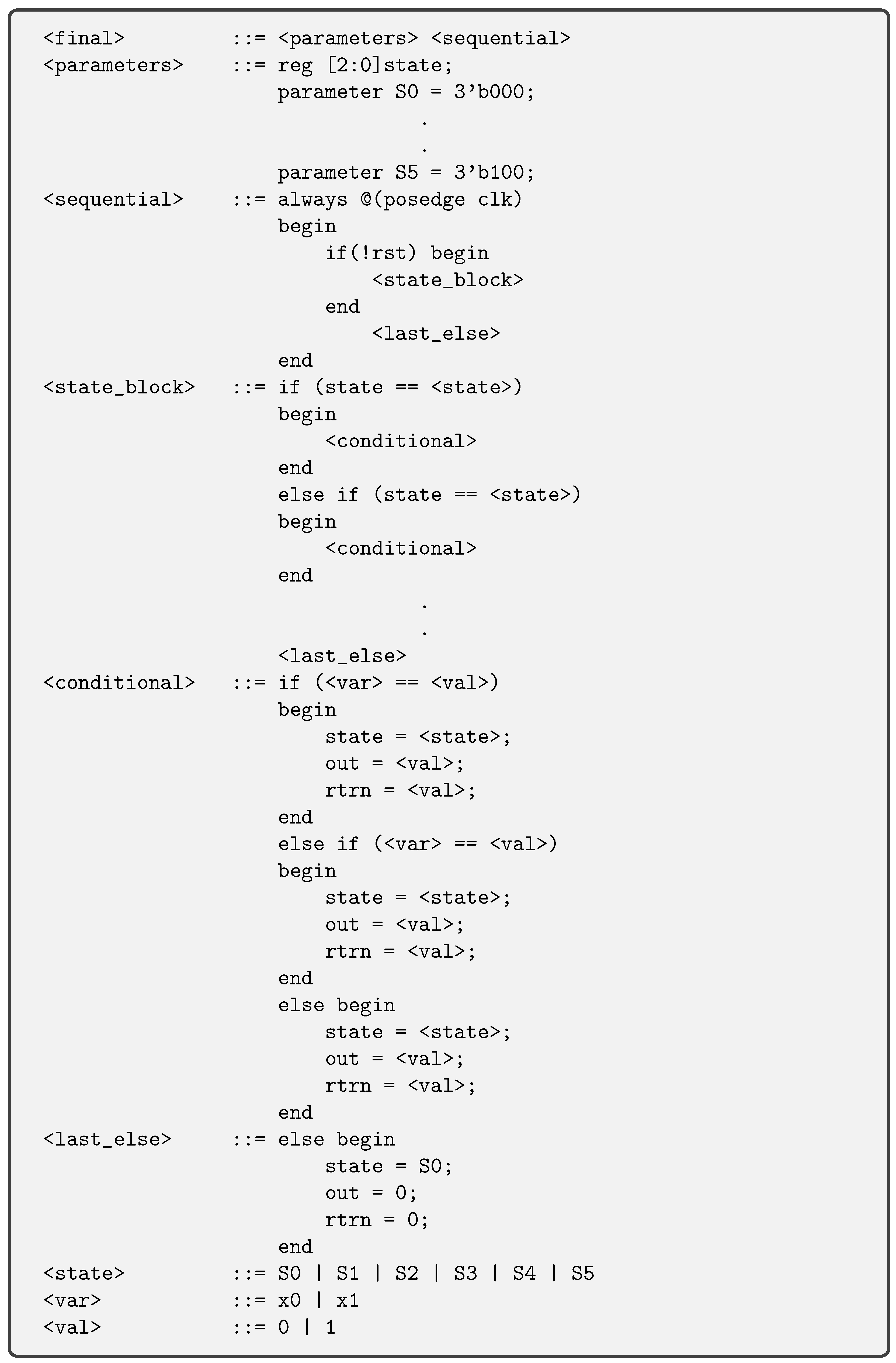
The grammar used in this study is shown in Figure 5. This work focuses on evolving the HDL code for a 6-state MSD, which is more complex than the previously evolved FSM for a 6-bit SD discussed in [44]. The increased complexity arises from the MSD’s ability to track two sequences. We have evolved not only the system’s next state and the values of two respective outputs—confirmation of payment and refund amount—but also the current state, input variables, and the values for input variables, which were not addressed in the previous work. This grammar facilitates the generation of the HDL module, which is simulated using Icarus Verilog.

The first production rule connects the $<parameters>$ to $<sequential>$, where $<parameters>$ defines hardcoded state parameters by assigning them 3-bit values. The $<sequential>$ block contains the entire always block that implements the FSM. Within this always block, if the system is not undergoing a reset, the $<states$_$block>$ selects the appropriate if–else if statement according to the system’s current state (which is also evolved) and then enters $<conditional>$. The $<conditional>$ block further selects the respective if–else if condition based on the evolved input variable and its evolved value, assigning the evolved next state and evolved outputs to the system. If the system is in a reset state, $<last$_$else>$ is chosen within the always block, assigning hardcoded values to the next state and outputs, as specified in the grammar. The last three non-terminals only have terminals on the RHS, which are used throughout to evolve the current state, next state, input variable and its value, and the value of the outputs.

In this work, the primary evaluation metric used during the evolutionary process is the fitness score. The fitness score measures how accurately an evolved individual solves the target FSM problem by comparing its outputs against the expected outputs for a predefined set of TCs.

A total of 16 TCs divided into 64 3-bit vectors (as shown in Section 5) are used, where each case represents a specific input sequence and the corresponding expected output behaviour. For each 3-bit vector that the evolved individual resolves correctly, it is awarded a score of ‘1’. If the output for a vector does not match the expected behaviour, a score of ‘0’ is assigned for that vector. The overall fitness score is computed by summing the individual scores across all 16 12-bit TCs or all 64 3-bit vectors. Therefore, the maximum achievable fitness score for an individual is ‘64’, indicating perfect performance on all TCs.

The overall fitness score F for an individual is calculated by summing the scores across all 64 3-bit vectors and is defined as:

$$F=\sum _{i=1}^N{s}_i$$

(1)

where the following are used:

• $N=64$ is the total number of 3-bit vectors;
• $s_i=1$ if the individual’s output for vector i matches the expected output;
• $s_i=0$ otherwise.

6.2. Experiments and Results Using Tournament Selection

In the first set of experiments, using TS as the parent selection method, the initial experiment was conducted with a population size of 1000 over 30 generations. The system took 59 min and 36 s to successfully evolve only two solutions across thirty runs, as reported in Table 2. Somewhat arbitrarily, we set a target of 25/30 successful runs; if a setup produces fewer than that, we consider the setup inadequate. In Table 2, blue text indicates the training and test success rate on unsuccessful runs, while green text indicates the training and test success rate greater than 25. No further experiments were run once we managed a success rate greater or equal to 25.

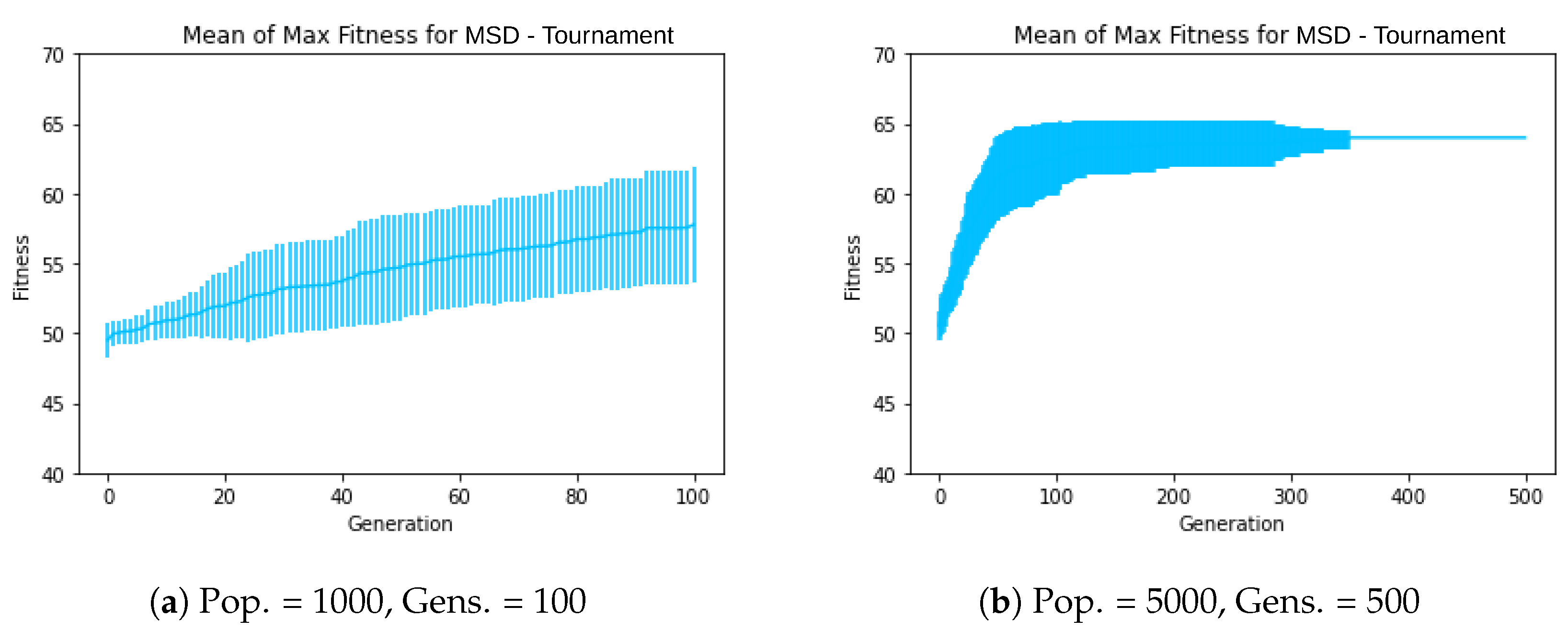
For this first experiment, the mean of the maximum fitness graph (all graphs for these experiments are provided in the SM, showing the mean maximum fitness scores of evolved circuits over 30 runs across the maximum number of generations) revealed consistently increasing error bars over the generations (as seen in the subsequent experiment shown in Figure 6a). Noting the significant variability in solutions indicated by the large error bars, the number of generations increased to 100, achieving a success rate of 6/30 and taking the execution time of 177 min and 42 s, almost three times the previous experiment. The resulting graph continued to show large error bars, as illustrated in Figure 6a. The number of generations was then further increased to 500, taking an execution time of 870 min and 23 s and resulting in a success rate of 20/30. Although the results did not improve fivefold with the increased number of generations, the error bars remained substantial.

The number of generations was further increased to 1000, resulting in a success rate of 23/30, taking execution time of 1732 min and 53 s. The error bars on the graph were significantly reduced. We experimented with swapping these values to explore whether a larger population size with fewer generations might yield better results. The population size was set to 5000, and the number of generations was reduced to 100 (thus keeping the total number of individuals the same). With these settings, we achieved the same success rate of 20/30, with an execution time of 872 min and 45 s. However, the error bars indicated considerable variability in the solutions, with no clear trend toward saturation.

We then kept the population size at 5000 and increased the number of generations to 500. This configuration took execution time of 4348 min and 15 s and led to a perfect success rate of 30/30, with the system reaching this rate around 350 generations, as shown in Figure 6b.

Since the dataset used for training is the only one available for the test success rate, the entire dataset was used for training and testing. The respective success rate of the evolved solutions on the test dataset is indicated in the same column in Table 2, showing perfect accuracy for all evolved solutions.

6.3. Experiments and Results Using Lexicase Selection

All settings were kept consistent with the TS method, and the first experiment was conducted with a population size of 1000 across 30 generations, repeated over 30 runs. This resulted in a training and test success rate of 09/30, taking an execution time of 57 min 42 s, as shown in Table 2. Since this is not an acceptable success rate, we increased the number of generations to 100. This adjustment led to a success rate of 17/30, with an execution time of 178 min and 41 s, which is approximately three times higher than the TS method under the same generation setting, as seen in Table 2. Despite this improvement, the graph still displayed large error bars and a lack of saturation, leading to a further increase in the number of generations to 500. This change resulted in a success rate of 29/30, taking an execution time of 867 min and 56 s, again significantly outperforming the TS method under identical hyperparameter settings. No further experiments were conducted because this success rate was nearly perfect. The resulting graph showed the mean of the maximum fitness value approaching saturation, with consistently narrowing error bars.

It can be seen that in evolving FSMs, where multiple diverse and sometimes conflicting TCs must be satisfied, LS outperforms TS by preserving individuals that solve specific difficult cases. Unlike TS, which favours generalist individuals with good average performance and risks losing useful specialists early, LS evaluates performance case-by-case, maintaining a richer diversity of FSM behaviours. This diversity is crucial for complex FSM evolution, where different transitions and outputs may be optimised at different stages. As a result, LS enables better exploration and often leads to higher-quality FSM solutions.

Incorporating both LS and TS, the proposed method is highly scalable to larger and more complex FSMs. However, scaling may require greater computational and evolutionary resources. To adapt this methodology for larger FSMs, modifications to the grammar, training dataset, and testbench would be necessary. For example, expanding the current FSM to support more than two products would require a complete restructuring of the dataset and FSM, alongside corresponding updates to the grammar and testbench. Future work will focus on scaling this methodology to enable the evolution of more complex and larger FSMs.

7. Evolved Solution FSM

7.1. Code and Transition Analysis

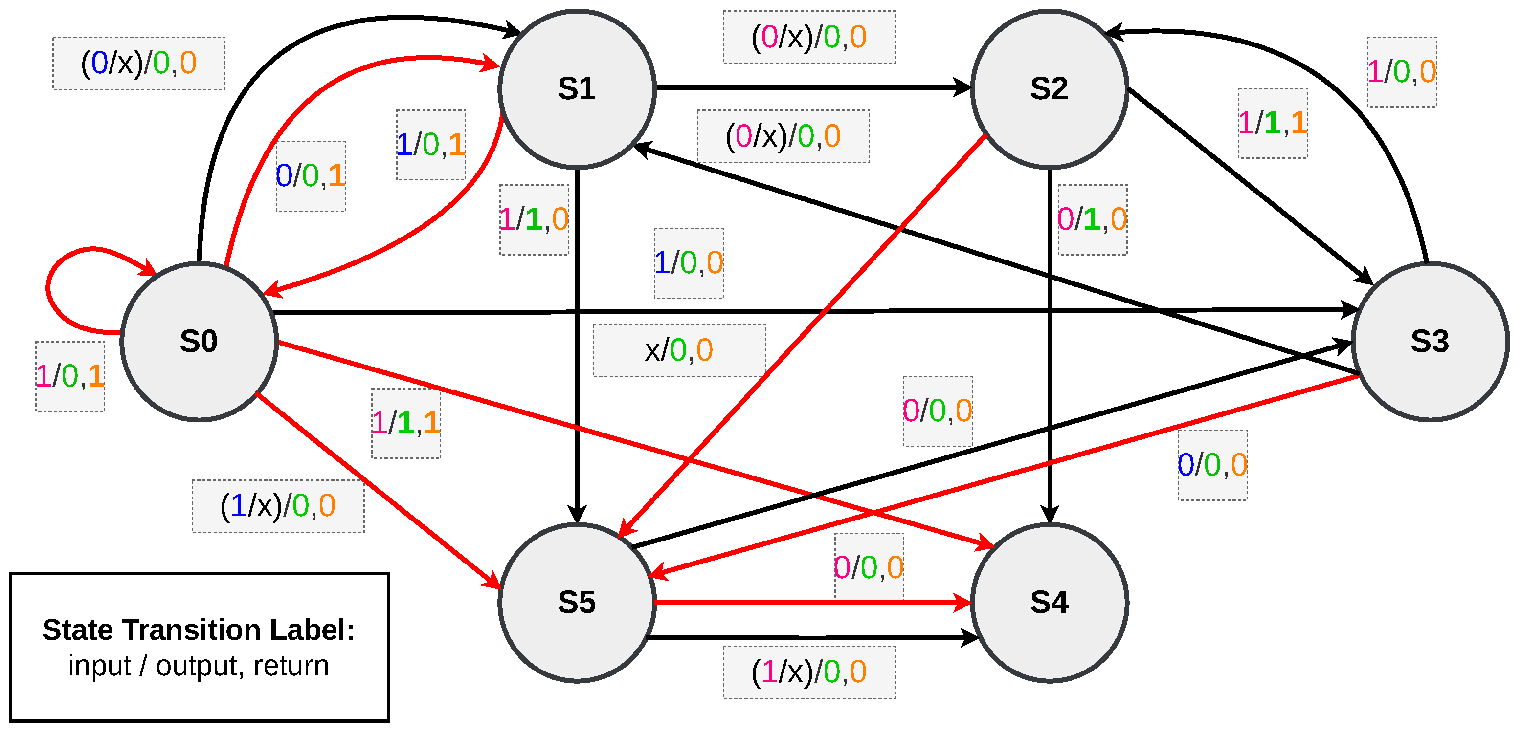
FSM of one of the perfectly evolved solution circuits in SV is shown in Figure 7. This FSM is taken from the solution circuits generated using LS, and the experiment has a top success rate of 29/30. In this evolved FSM, all state transitions and their conditions are automatically generated through the evolutionary process discussed earlier. The FSM structure includes six states, named S0 to S5, aligning with the human-designed FSM presented in Section 2. Notably, the evolved solution exhibits a broader set of transitions, showcasing the creative and exploratory nature of the GE.

The FSM shows transitions in both black and red colours. The black transitions are the ones in use that occur during execution based on the testbench inputs. The red transitions exist in the code but are never triggered during real operation. These extra transitions show how the evolved system can explore a wider range of possible behaviours and add flexibility to the design.

In this structure, transitions originating from state S0 based on x1, indicated in dark pink within the transition labels, are not functionally utilised, as x1 is not active during S0 according to the testbench configuration. These transitions are marked in red in the FSM diagram to indicate that they remain inactive in this context. Similarly, transitions from states S1 through S5 based on x0, represented in blue within the transition labels, are also non-operative in actual execution, as x0 is only defined during the initial cycle in S0. The colour scheme used for input bits in the transition labels is consistent with the human-designed FSM in Figure 1, aiding in visual continuity and interpretability.

Some transitions are labelled with combined conditions such as ‘(0/x)’ or ‘(1/x)’. These originate from broader else blocks in the evolved code, as opposed to the more precise else if chains used in the human-designed solution. While this approach may appear less constrained, it highlights the flexibility of the evolved FSM to accommodate various input combinations without compromising functionality.

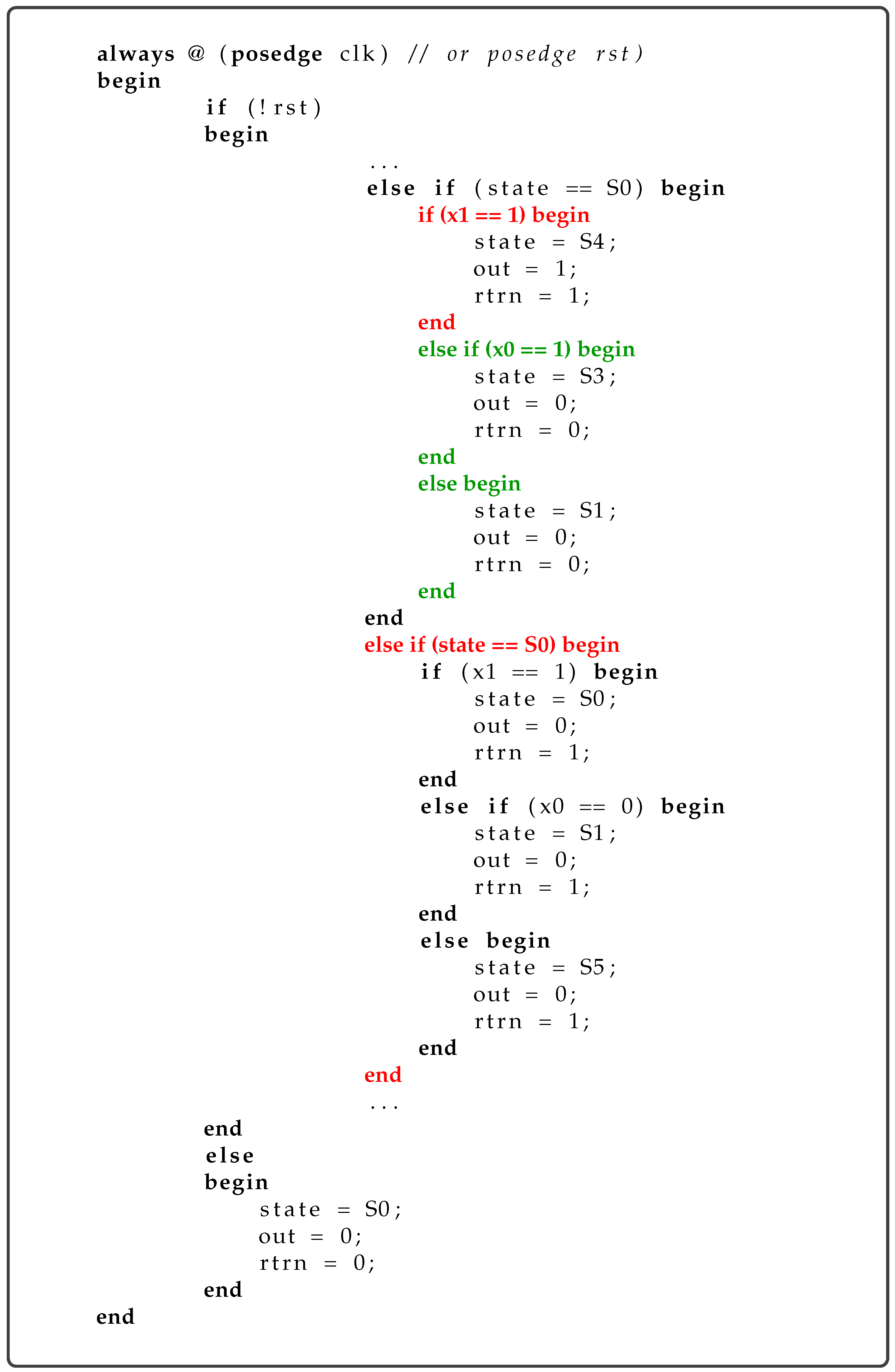
An interesting aspect of the evolved FSM is the presence of repeated or overlapping state conditions. For instance, as shown in Figure 8, state S0 is defined in two separate blocks, both beginning with state == S0. Given the sequential nature of the code, only the first such block is ever executed during runtime, while the second block (highlighted in red) remains extraneous. This is reflected in the FSM diagram in Figure 7, where transitions linked to the second block are highlighted in red. These extra structures, although inactive, are byproducts of the evolutionary search process and illustrate the system’s openness to exploring alternative representations.

Additionally, certain conditional checks, such as x1 == 1, appear in S0, despite x1 being undefined during that state. It can be seen in Figure 8 that the conditional statement based on x1 == 1 in the first block based on S0 will never execute, yet is highlighted in red. The remaining part of this block, which will be able to execute, is highlighted in green. Likewise, some input checks like x1 == 0 occur multiple times within the same state, as can be seen in the transitions from S5, where two transitions are based on the same input and output labels. However, one is valid and the other is not. These repetitions and overlaps are not errors but rather emergent outcomes of the grammar-based evolutionary system, which emphasises functionality and completeness over stylistic minimalism. They underscore the potential of GE to generate circuits that are not only correct but also adaptable and structurally diverse.

Thus, while the evolved FSM performs correctly on all evaluated TCs, its code also reflects the flexibility and exploratory nature of the evolutionary process, resulting in additional transitions and structures that, although not activated under current testbench constraints, demonstrate the system’s capacity to adapt and generalise beyond strictly defined scenarios.

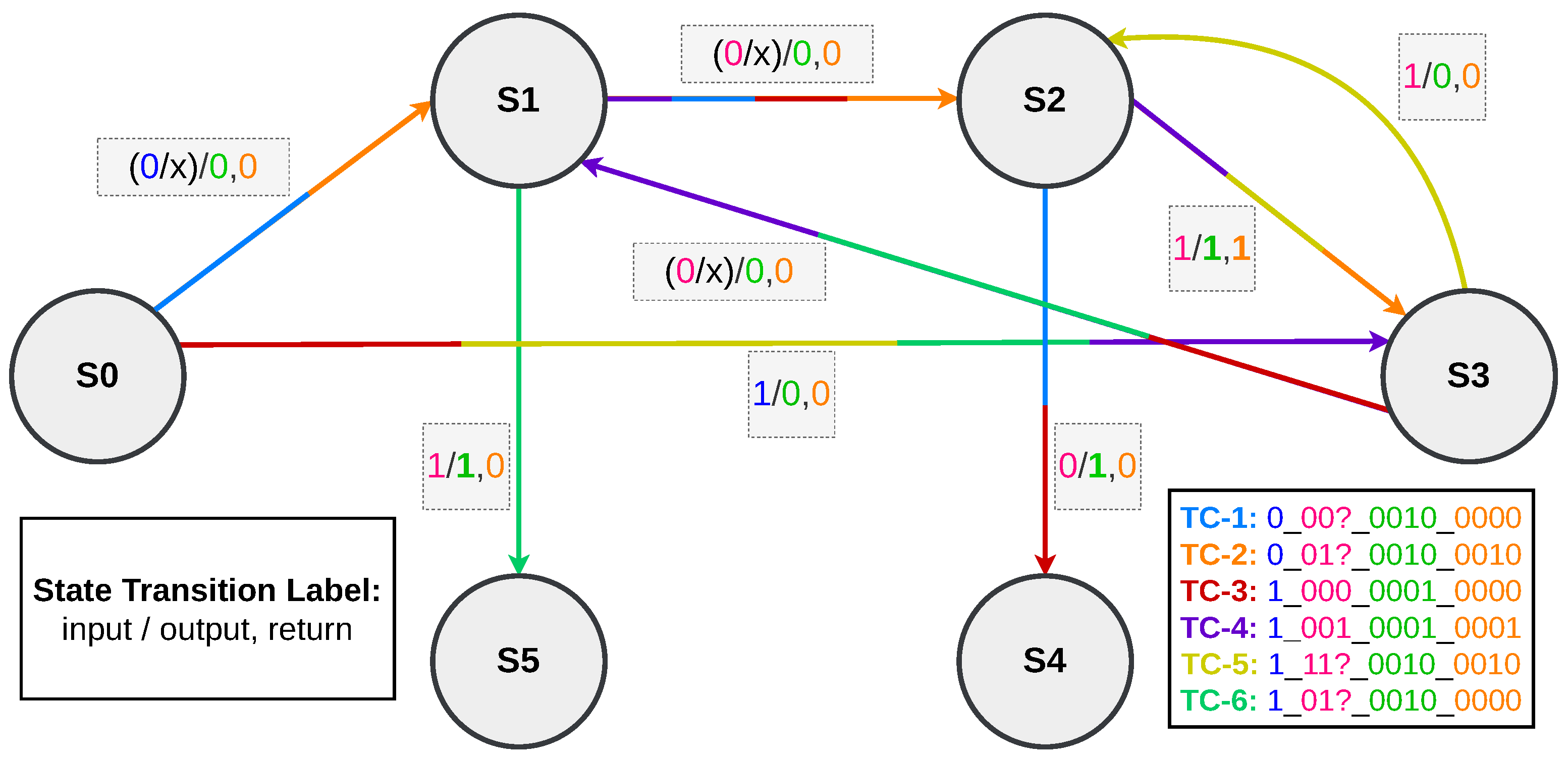
7.2. Test Case Mapping onto the Evolved FSM

After the FSM is evolved, its functionality is validated by mapping the six TCs (five of which were defined earlier in Section 5 and shown in Figure 4, the dataset generation process), onto the evolved state machine. These TCs represent various user interactions with the vending machine, covering all valid input-output behaviours. Each TC is shown in a unique colour on the FSM diagram in Figure 9 to clearly highlight the path it follows through the states.

The mapping uses the following colour scheme for the six TCs:

• Azure for TC-1;
• Orange for TC-2;
• Maroon for TC-3;
• Purple for TC-4;
• Citrine yellow for TC-5;
• Parrot green for TC-6 (an additional test case not shown in the original dataset figure).

Each coloured path corresponds to a valid sequence of transitions based on the inputs defined in the respective test case. For example, in TC-2, the system begins in state S0, detects a water selection x0 = 0, and proceeds to state S1. From there, it transitions through additional states depending on the payments made using x1, until the total payment matches the product cost.

The same logic applies to the fizzy drink selection path, such as in TC-4, which begins with x0 = 1 in S0 and continues through states like S3, S1, and S2, depending on the combination and order of EUR 0.50 and EUR 1 coins. It finally ends at S3 with the delivery of the product and a return change of EUR 0.50. In each TC, the state transitions and output responses follow the correct timing and behaviour, as expected from the FSM.

The additional TC, TC-6, is shown in parrot green in Figure 9 and follows the input and output pattern ‘1_01x_0010_0000’. This TC is specifically included to highlight the use of state S5, which is not involved in the first five TCs. By showing a path that passes through S5, the evolved FSM demonstrates its coverage of all relevant states and confirms its flexibility in handling less common but still valid scenarios. The transition labels in this figure also follow the same colour coding as used in the dataset generation figure (Figure 4).

Even though the evolved FSM shown in Figure 7 includes some transitions that are not used during execution, these do not affect the system’s operation. The testbench restricts the inputs per cycle, so only the correct transitions are activated. The evolved FSM, therefore, completes all TCs correctly and achieves the maximum fitness score of 64, meaning it delivers the right outputs for all 64 input vectors derived from the dataset.

8. Logic Synthesis

After successfully generating HDL codes for MSDs using both TS and LS, the evolved solutions (successful candidates from each run) were synthesised and compared with the synthesis of the Gold Circuit. For this, 29 and 30 solution circuits, which are the best of the run from each of LS and TS, respectively, where the best success rates were achieved, were taken towards the synthesis, as shown in Table 2. The synthesis process employed Complementary Metal–Oxide–Semiconductor (CMOS) GPDK technologies at 45 nm, 90 nm, and 180 nm nodes, using the Cadence Genus synthesis tool at a clock frequency of 100 MHz. The reset signal was configured to the ideal network in the constraints file. For all three GPDK technologies, synthesis was performed under both Fast Corner (FC) and Slow Corner (SC) conditions. FC represents the most optimal operational environment for the circuit, based on specific temperature and supply voltage settings, while SC denotes the least favourable conditions. The temperature and voltage values used in these designs are detailed in

Table 3. Nominal temperature and supply voltage for logic synthesis of relevant technologies.

Parameters	45 nm		90 nm		180 nm
	FC	SC	FC	SC	FC	SC
Temperature (°C)	0	125	0	125	0	125
Voltage (V)	1.32	1.08	1.1	0.9	1.98	1.62

.

Table 4. A comparison of synthesis reports generated using GPDK 45 nm, 90 nm, and 180 nm on FC and SC in terms of the best (minimum), average, standard deviation, median, worst (maximum), and statistical hypothesis test’s p-values of area (measured in the unit of number of cells) and PDP (measured in the unit of milliwatt-picoseconds) between the Gold and evolved circuits using TS and LS.

			Gold Circuit	Parameter	45 nm		90 nm		180 nm
					FC	SC	FC	SC	FC	SC
				Area	19	26	20	20	17	17
				PDP	115.7	80.56	64.51	79.2	356.5	483.1
45 nm	Parameter	Evolved Through TS
		FC						SC
		Best	Mean	STD	Med.	Worst	p-value	Best	Mean	STD	Med.	Worst	p-value
	Area	18	24.66	4.84	25	37	5.26e-07	21	29.3	4.78	30	40	7.2e-04
	PDP	106.1	126.9	11.08	125.85	157.46	5.44e-06	72.08	88.07	9.26	87.64	110.6	1.21e-04
	Parameter	Evolved Through LS
		FC						SC
		Best	Mean	STD	Med.	Worst	p-value	Best	Mean	STD	Med.	Worst	p-value
	Area	12	25.93	4.52	26	33	5.47e-09	19	31.03	4.52	31	38	1.86e-06
	PDP	110.8	135.62	14.81	131.96	160.78	6.92e-08	66.6	94.95	13.47	93.6	117.15	3.57e-06
90 nm	Parameter	Evolved Through TS
		FC						SC
		Best	Mean	STD	Med.	Worst	p-value	Best	Mean	STD	Med.	Worst	p-value
	Area	17	24.4	4.03	24.5	33	1.69e-06	17	24.4	4.08	24.5	33	2.07e-06
	PDP	58.3	64.47	4.14	63.38	77.67	0.96	72.21	79.75	5.79	78.32	96.81	0.607
	Parameter	Evolved Through LS
		FC						SC
		Best	Mean	STD	Med.	Worst	p-value	Best	Mean	STD	Med.	Worst	p-value
	Area	13	25.55	4.29	25	33	1.46e-07	13	25.52	4.19	25	33	1.02e-07
	PDP	57.2	67.4	7.40	64.75	81.48	0.047	70.54	83.42	9.56	80.04	101.58	0.025
180 nm	Parameter	Evolved Through TS
		FC						SC
		Best	Mean	STD	Med.	Worst	p-value	Best	Mean	STD	Med.	Worst	p-value
	Area	17	23.5	3.86	23.5	31	4.14e-10	16	23.7	3.92	24	31	2.93e-10
	PDP	317.9	365.6	24.49	360.77	440.1	0.05	404.8	471.6	40.57	471.9	596.42	0.13
	Parameter	Evolved Through LS
		FC						SC
		Best	Mean	STD	Med.	Worst	p-value	Best	Mean	STD	Med.	Worst	p-value
	Area	12	24.45	4.28	24	33	3.98e-10	16	24.1	3.78	24	32	7.52e-11
	PDP	319.6	377.21	41.84	369.2	454.78	0.013	418.5	503.1	59.34	483.47	614.37	0.08

presents a comparison of synthesis reports between the Gold MSD and the MSDs evolved using TS and LS, focusing on area (measured in the number of cells) and Power Delay Product (PDP). The PDP, calculated as the product of power and delay, is a crucial metric in evaluating IC design performance, given the inherent trade-offs between power consumption and delay. The unit of PDP is milliwatt-picoseconds (mWps). The comparisons in Table 4 are organised by the relevant GPDK technology, highlighted in three different shades of maroon; the lighter the shade, the smaller the GPDK technology. For instance, the synthesis reports of the Gold Circuit under FC and SC conditions using 45 nm technology are compared against those of the evolved circuits using the same technology under TS and LS. This method is similarly applied to 90 nm and 180 nm technologies.

For each technology, the Gold Circuit’s metrics under FC and SC conditions are compared with the best (minimum), mean/average (AVG), median, and worst (maximum) values among the 29 perfect solution circuits evolved through LS and the 30 solution circuits evolved through TS. The table also includes the standard deviation (STD) among all values. At least one synthesised solution circuit for each technology generated through the proposed system has performed either better than the Gold Circuit, highlighted in green, or equal to the Gold Circuit, highlighted in blue. It can be seen that only one value out of 24 values is highlighted in blue, and the rest are shown in green, which means that evolution has produced a better result than the Gold Circuit under almost every circumstance.

Moreover, to show if there is a statistically significant difference between the synthesis reports of gold and evolved circuits, p-values extracted from the statistical hypothesis test named one-sample t-test are also given, where the Gold Circuits are compared with evolved circuits. Since the p-value if less than or equal to 0.05 indicates that there is a significant difference between the Gold Circuit and the group of circuits evolved under the specific technology, it is shown in bold and orange colour that for 20 out of 24 values of area and PDP values taken from evolved circuits, the null hypothesis can be rejected. There is a significant difference compared with the values of the Gold Circuit. There are only four values where the null hypothesis cannot be dismissed, and we have to note that there is no significant difference between the Gold Circuit’s values and the mean values taken from the group of 30 or 29 circuits for a specific technology. Given this, we can safely say that most of the circuits are significantly different and better than the Gold Circuit, and we can generate better solutions automatically through evolutionary ML, which is the primary goal of this work.

Solutions evolved through LS achieve a higher success rate compared with TS. The performance of the synthesised designs from LS also surpasses those from TS, since three out of four values with a p-value greater than 0.05 belong to TS. This leads the authors to recommend LS as the preferable parent selection technique for evolving complex sequential circuits.

A two-sample t-test is run between the synthesis reports of the groups of circuits evolved through LS and TS, and the extracted p-values are shown in

Table 5. T-test results run on the groups of solution circuits evolved through LS and TS under the relevant GPDK technologies.

Parameter	45 nm				90 nm				180 nm
	FC		SC		FC		SC		FC		SC
	Area	PDP	Area	PDP	Area	PDP	Area	PDP	Area	PDP	Area	PDP
p-value	0.304	0.014	0.157	0.027	0.293	0.077	0.304	0.082	0.376	0.202	0.689	0.022

. The values less than 0.05 show a significant difference between the two groups, shown in bold and red, while the rest are in bold and green. So, it can be seen that although LS performed much better than TS in terms of evolutionary success rate, the circuits evolved through both are pretty much similar according to the synthesis reports, yet acceptable.

9. Conclusions and Future Work

This work introduces the evolution of synthesisable HDL codes for a single-input, multi-output MSD using GE and two parent selection methods: TS and LS. Although these parent selection methods and GE are well-established techniques, they are combined here to evolve the FSM of a real-life MSD, which is complex and hard to evolve and speaks to the novelty of the presented system. The evolved MSD is applied to a practical vending machine scenario, covering the entire process from product selection through payment to delivery. Using the evolved MSD designs in a vending machine scenario, the study validates the effectiveness of the evolutionary methods in generating practical, real-world solutions. It also shows the potential for these methods in other complex systems requiring similar state management capabilities, such as robotics.

The results demonstrate that LS significantly outperforms TS in evolving a sequential Mealy machine in terms of success rate and computational efficiency. The Gold standard and evolved circuits are synthesised to validate the practical application using GPDK at 45 nm, 90 nm, and 180 nm. These syntheses confirm that the circuits evolved to represent a significant step forward in automated chip design and manufacturing. Notably, at least one evolved circuit outperforms the Gold Circuit using either TS or LS. This study is the first to evolve synthesisable HDL codes for MSDs.

Future work will focus on evolving more complex circuits, such as multi-input and multi-output MSDs. In addition, another future direction will consider exploring the systematic hyperparameter tuning techniques to optimise evolutionary ML approaches, such as GE, which will likely improve overall system performance. We will also investigate using some other implementations of GE than GRAPE, such as Grammatical Algorithms in C++ for Evolution (GRACE), where the LS can be compared with the results of the approach used here.