A Semi-Supervised-Learning-Aided Explainable Belief Rule-Based Approach to Predict the Energy Consumption of Buildings

Abstract

Predicting the energy consumption of buildings plays a critical role in supporting utility providers, users, and facility managers in minimizing energy waste and optimizing operational efficiency. However, this prediction becomes difficult because of the limited availability of supervised labeled data to train Artificial Intelligence (AI) models. This data availability becomes either expensive or difficult due to privacy protection. To overcome the scarcity of balanced labeled data, semi-supervised learning utilizes extensive unlabeled data. Motivated by this, we propose semi-supervised learning to train AI model. For the AI model, we employ the Belief Rule-Based Expert System (BRBES) because of its domain knowledge-based prediction and uncertainty handling mechanism. For improved accuracy of the BRBES, we utilize initial labeled data to optimize BRBES’ parameters and structure through evolutionary learning until its accuracy reaches the confidence threshold. As semi-supervised learning, we employ a self-training model to assign pseudo-labels, predicted by the BRBES, to unlabeled data generated through weak and strong augmentation. We reoptimize the BRBES with labeled and pseudo-labeled data, resulting in a semi-supervised BRBES. Finally, this semi-supervised BRBES explains its prediction to the end-user in nontechnical human language, resulting in a trust relationship. To validate our proposed semi-supervised explainable BRBES framework, a case study based on Skellefteå, Sweden, is used to predict and explain energy consumption of buildings. Experimental results show 20 ± 0.71% higher accuracy of the semi-supervised BRBES than state-of-the-art semi-supervised machine learning models. Moreover, the semi-supervised BRBES framework turns out to be 29 ± 0.67% more explainable than these semi-supervised machine learning models.

1. Introduction

Building energy consumption contributes significantly to climate change [1]. Approximately 40% of the world’s energy is consumed by the building sector [2]. Furthermore, significant population expansion has raised the need for energy in buildings [3]. Therefore, in order to hasten the shift to sustainable building methods, buildings must be energy efficient. Predictive analytics of building energy consumption are an effective method of achieving this energy efficiency [4]. Based on the insights provided by such predictive consumption, utility companies, consumers, and facility managers can take necessary steps to make their buildings energy efficient [5]. Such efficiency is crucial to reduce energy costs and increase the energy security of buildings [6]. Moreover, energy prediction of buildings aids in the implementation of urban greening policies [7].

Meaningful prediction is offered by Artificial Intelligence (AI) models, such as machine learning and deep learning models, by discovering hidden pattern from historical energy consumption data [8]. These AI models learn from a large amount of labeled energy consumption data through supervised learning to offer such predictions [9]. However, obtaining labeled data for building energy consumption prediction is often challenging due to the high cost and effort involved in collecting accurate ground-truth measurements [10]. Many energy datasets lack sufficient labels because of sensor deployment limitations, data privacy concerns [11], and manual annotation burdens [10,12]. This scarcity of supervised labeled data hinders the development of robust and scalable AI models for energy consumption prediction in diverse building environments. A labeled dataset can be imbalanced as well. Hence, using unlabeled energy data to train AI models can overcome the scarcity, inaccessibility, and imbalance issues of labeled energy data. Training an AI model with a small number of labeled data points and a large number of unlabeled data is called semi-supervised learning (SSL) [13,14,15,16]. SSL learns knowledge from a small number of labeled data to meaningfully label a large amount of unlabeled data. Thus, SSL facilitates the training of an AI model by capitalizing on the abundance of unlabeled data, resulting in higher prediction accuracy [12]. SSL methods are divided into five groups [17]: (a) deep generative methods, (b) consistency regularization methods, (c) graph-based methods, (d) pseudo-labeling methods, and e) hybrid methods. Semi-supervised Variational Autoencoders (VAEs), and Generative Adversarial Networks (GANs) are examples of deep generative methods. Although such methods generate new training examples, achieving optimal results for both generative task and downstream task is difficult. Virtual Adversarial Training (VAT) [16] is an example of consistency regularization methods. As a consistency-based SSL method, a novel Semi-supervised Universal Graph Representation Learning (SUGRL) framework was proposed by [18]. This framework performs graph classification in semi-supervised settings when graphs originate from diverse domains with heterogeneous structures. For this purpose, it learns domain-invariant representations through contrastive self-supervised learning and adversarial domain alignment. This method significantly improves generalization across domains using limited labeled data and abundant unlabeled graphs. Another consistency-based SSL method, Rationale-Informed Graph Neural Network (RIGNN), was proposed by [19]. This method identifies and leverages task-relevant subgraphs (rationales) to enhance classification robustness. By disentangling discriminative information from noisy or out-of-distribution data, RIGNN improves generalization under open-world and label-sparse settings. This work underscores the importance of interpretability and selective representation in advancing semi-supervised graph learning. Although these consistency-based methods construct consistency constraints with clear assumptions, data augmentation and perturbation methods may not be fully reliable [17]. Graph Neural Network (GNN) and Autoencoder-based models fall under graph-based methods. However, conventional graph structures are inherently limited to modeling pairwise relationships, which may not fully capture the higher-order dependencies often present in complex real-world data. To address this limitation, Hypergraph-enhanced Dual Semi-supervised Graph Classification (HDSGC) has been proposed as a powerful alternative that incorporates both graph and hypergraph representations to better capture complex and high-order relationships among data points [20]. HDSGC utilizes hyperedges to represent multi-node interactions, enriching the contextual information available for learning. It introduces a dual semi-supervised learning strategy that jointly optimizes node classification on both graph and hypergraph views, leveraging the complementary strengths of each structure. This method achieves improved performance on graph classification tasks with limited labeled data by enhancing representation learning through multi-relational modeling. Although such methods learn more information with graphs, building relationship between training samples may not be always accurate [17]. Disagreement-based models and self-training models fall under pseudo-labeling methods. As an iterative self-training strategy, SemiEvol—Semi-supervised Fine-tuning for LLM Adaptation [20]—leverages both labeled and high-confidence pseudo-labeled data to progressively fine-tune Large Language Models (LLMs). By integrating teacher–student paradigms with dynamic data selection, SemiEvol facilitates robust adaptation across diverse tasks under semi-supervised conditions. Although these methods produce pseudo-labels for unlabeled examples using labeled examples, such pseudo-labels may become noisy [17]. Interpolation Consistency Training (ICT) [21], MixMatch [22], ReMixMatch [23], and FixMatch [24] are examples of hybrid methods. A hybrid SSL framework was introduced through Semi-supervised Active Learning for Graph-level Classification [25], which combines semi-supervised learning with active learning to efficiently label graph-structured data. It strategically selects the most informative graph instances to be labeled, thereby maximizing learning performance with minimal annotation cost. By leveraging both labeled and unlabeled graphs during training, the method balances exploration and exploitation to enhance graph-level classification. This approach demonstrates state-of-the-art results by integrating uncertainty estimation with structure-aware sampling strategies. Another hybrid SSL method was proposed by [26], which combines curriculum learning with pseudo-labeling to improve node classification in graph-based SSL. This method iteratively selects pseudo-labels for unlabeled nodes based on both confidence and the complexity of the node’s features, forming a hybrid curriculum. This curriculum-guided strategy helps the model progressively learn from easier to harder instances, leading to better generalization and faster convergence. This approach outperforms traditional pseudo-labeling methods by incorporating a structured learning process that adapts to the evolving uncertainty of the model [26]. Although such hybrid methods offer more robustness and efficiency, the size of such methods is larger due to integration of various learning strategies. Moreover, based on output, SSL is of four types [27]: semi-supervised classification, semi-supervised clustering, semi-supervised dimension reduction, and semi-supervised regression. The continuous value of energy consumption of a building needs to be predicted [28]. However, among these four categories, semi-supervised regression research to predict value of a continuous variable is relatively scarce [29].

Prediction can be obtained in two ways: a data-driven approach and knowledge-driven approach [30]. A data-driven approach learns from data to predict output. Machine learning, a data-driven approach, extracts actionable insight from training data through statistical technique [31]. Deep learning model also learns hidden representation by applying a representation learning method on preprocessed raw data [32]. Various data-driven approaches, such as, Random Forest (RF) [33], Light Gradient Boosting Machine (LightGBM) [34], Automated Machine Learning (AutoML) [35], and Artificial Neural Network (ANN) [36] are employed to predict energy consumption of buildings. However, a data-driven approach can predict misleading output due to biased or erroneous training dataset [37]. On the other hand, a knowledge-driven approach obtains a predictive output based on knowledge, which is represented by rules [38]. This approach is constituted by an expert system consisting of two components: a knowledge base and an inference engine. The knowledge base represents knowledge of the relevant domain or application area, and the inference engine performs reasoning over this knowledge base to infer predictive output. Examples of knowledge-driven approaches include the Belief Rule-Based Expert System (BRBES), MYCIN [39], and fuzzy logic. A fuzzy logic algorithm was proposed by [40] to predict short-term energy consumption in individual buildings. Their proposed fuzzy logic system comprises fuzzification, rule definition, inference, and defuzzification steps, enabling effective day-to-day consumption predictions. Another study combined a fuzzy rule-based prediction system with multi-objective evolutionary optimization to predict residential building energy consumption [41]. The BRBES was employed by [37] to predict energy consumption of buildings in a transparent manner. They trained the BRBES with evolutionary optimization using supervised labeled data to improve accuracy. A knowledge-driven approach is not dependent on training data [37]. Its knowledge base is formulated by experts with relevant domain knowledge. Hence, a knowledge-driven approach is free from the risk of bias or errors in a training dataset [37]. In contrast to an ad hoc training dataset, property managers are more inclined to believe a prediction output that is based on knowledge pertaining to the energy consumption domain [37]. Moreover, domain knowledge can capture the complex interplay among underlying physical and operational factors of a building, which influence its energy use [42]. Such factors include building design, occupancy patterns, HVAC (Heating, Ventilation, and Air Conditioning) systems, and external environmental conditions. Therefore, we opt for the knowledge-driven approach to infer the prediction of energy consumption of buildings in this paper. Moreover, predictive energy consumption output can become erroneous due to wrong input data caused by human error or blank input data caused by human ignorance, resulting in uncertainties [43]. Such uncertainties are caused by imprecise or incomplete human knowledge [44,45]. Therefore, these uncertainties have to be addressed properly to uphold the prediction accuracy. The belief rule basis of the BRBES, formulated based on a belief structure, can capture uncertainties and nonlinear causal relationships [46]. This rule base of the BRBES, formulated by domain experts, represents knowledge of the energy consumption domain. In case of unavailability of some or all of the input data, the BRBES updates belief degrees of its rule base [47]. THe BRBES obtains its predictive output by applying Evidential Reasoning (ER) on the rule base [8,48]. Thus, the BRBES outperforms other knowledge-driven approaches in terms of handling uncertainties, especially those caused by ignorance [47]. Hence, as knowledge-driven approach, we employ the BRBES in this research to obtain predictive energy consumption output. By representing energy consumption domain knowledge through a rule base, the BRBES offers higher explainability [37]. However, it has lower accuracy compared to conventional machine learning models. To improve its accuracy, we jointly optimize both parameters and structure of the BRBES with the Joint Optimization of Parameter and Structure (JOPS) algorithm [49]. With this joint optimization using supervised labeled data, the initial BRBES transitions to the supervised BRBES. We continue to optimize this supervised BRBES until the confidence level of its accuracy reaches a certain threshold. After reaching this accuracy threshold, the supervised BRBES transitions to the “confident BRBES”. We then integrate SSL with this confident BRBES to train it with a larger synthetic dataset. For the SSL method, we employ the self-training model [50] in this research. As part of the self-training model, we perform data augmentation to synthetically create new unlabeled data through transformation of the existing labeled data points [51]. Through data augmentation, we add more training examples of energy consumption to address overfitting and poor generalization [52]. In this study, we employ two types of data augmentation: “weak” and “strong”. Weak augmentation involves mild transformation of the original data points within a predefined range to increase data variability and generalization. On the other hand, strong augmentation involves more complex transformation to create challenging training examples that force the prediction model to learn more robust features. First, we apply weak augmentation to synthetically generate new unlabeled energy consumption data with equal distribution within a predefined range for each antecedent attribute of BRBES. Thus, we ensure proper diversity and density of the unlabeled data, resulting in a balanced unlabeled energy dataset. We then employ the confident BRBES to assign pseudo-labels to the weakly augmented unlabeled data. Thus, with the self-training model, we ensure that the pseudo-labels are assigned by no model other than the BRBES. This makes the pseudo-labels representative of domain knowledge while handling associated data uncertainties. We then optimize the confident BRBES with both a labeled and a weakly augmented pseudo-labeled energy dataset. If the accuracy increases, the confident BRBES will transition to the “weakly semi-supervised BRBES”. We then apply strong augmentation to generate more complex unlabeled energy data. To assign pseudo-labels to these strongly augmented unlabeled data, we apply the weakly semi-supervised BRBES. We then optimize this weakly semi-supervised BRBES with labeled as well as weakly and strongly augmented pseudo-labeled energy data. If the accuracy increases through this optimization, the weakly semi-supervised BRBES will transition to “semi-supervised BRBES”. Thus, with this semi-supervised BRBES, we provide energy consumption prediction with improved accuracy by overcoming the scarcity and imbalance of supervised labeled data. After obtaining predictive energy consumption output with this semi-supervised BRBES, we provide an explanation and counterfactual of this output to the end user through a user interface. The explanation and counterfactual are prepared in nontechnical human language so that any layperson can understand them. The explanation and counterfactual, formulated based on domain knowledge, create a relationship of trust between our model and human user [37]. Thus, we propose a semi-supervised explainable BRBES framework to predict the continuous value of the energy consumption of buildings accurately in units of kilowatt-hour (kWh) despite the scarcity of labeled data while providing an explanation and counterfactual based on knowledge of energy consumption domain. Thus, we perform semi-supervised regression while also explaining the regression output. We evaluate the accuracy, explainability, and counterfactual of our proposed semi-supervised framework with relevant metrics. In terms of accuracy, our proposed framework outperforms the supervised BRBES through semi-supervised learning. This framework also offers higher accuracy than conventional machine learning models by dealing with data uncertainties and optimizing itself with JOPS. In terms of explainability, this framework outperforms machine learning models by providing domain knowledge-based explanation in human-understandable language. Moreover, we assess our proposed framework’s balance between explainability and accuracy with the Belief Rule-Based adaptive Balance Determination (BRBaBD) algorithm [37]. To achieve our research objective, we focus on the following four research questions in this paper:

• How to address the scarcity of supervised labeled training data of energy consumption? We employ SSL to overcome the scarcity of labeled energy data with weakly and strongly augmented pseudo-labeled data.
• What is the benefit of predicting with BRBES? The benefit is prediction based on knowledge of the energy domain while dealing with data uncertainties.
• Why and how to integrate self-training model with BRBES? For the SSL model, we employ self-training to obtain pseudo-labels of unlabeled energy data with the BRBES only. A mathematical model is proposed to combine self-training with the BRBES.
• How to make the output of BRBES trustworthy to a human user? We make the predictive energy consumption output of the semi-supervised BRBES trustworthy by explaining it in nontechnical human language to a user through a user interface. This explanation is based on knowledge of the concerned domain.

The remainder of the paper is structured as follows: Relevant works are presented in Section 2. We then demonstrate our proposed semi-supervised explainable BRBES framework in Section 3. In Section 4, we present our experimental results. These results are discussed in Section 5. We conclude the paper and present our future research direction in Section 6.

2. Related Work

In this section, the existing SSL methods, unlabeled data labeling techniques, as well as type of data and predictive output are briefly covered. Then, we explain the motivation of the research.

2.1. SSL Methods

Sahoo et al. [11] employed an SSL approach to predict COVID-19 cases accurately from digital chest X-rays and Computed Tomography (CT) scans. Their proposed COVIDCon algorithm consisted of data augmentation (weak and strong), consistency regularization, and multi-contrastive learning. However, COVIDCon algorithm’s classification is based on multi-contrastive learning, with no consideration of knowledge related to COVID-19 domain. Moreover, this algorithm performs classification of images instead of regression over numerical input values. No explanation is provided by COVIDCon in support of the predictive diagnosis of COVID-19. Sahoo et al. [12] proposed a new multi-contrastive semi-supervised learning algorithm “MultiCon” to classify drug function into 12 categories by analyzing the features of two-dimensional images of drug chemical structure. This algorithm used multi-contrastive loss with consistency regularization to predict drug function. However, this algorithm’s multi-contrastive learning approach distinguishes image features through clustering. It does not take into account domain knowledge of drug function. Moreover, this algorithm is restricted to image classification only rather than numerical data regression. “MultiCon” also does not explain the rationale in support of its predictive output on drug function. Li et al. [53] proposed a new semi-supervised learning methodology Mixup Contrastive Mixup (MCoM) to address the imbalanced data problem in tabular cyber security datasets. To tackle this imbalance, their proposed MCoM employed triplet mixup data augmentation on the minority (vulnerable) class. Then they used contrastive and feature reconstruction loss to train the encoder and the decoder. They used a label propagation technique to pseudo-label the subset of the unlabeled data. For the predictor, they used Multi-Layer Perceptron (MLP). However, MLP is a data-driven approach, with no consideration of knowledge of cyber security domain. MCoM performs classification of security data instead of regression. Moreover, security classification output is not explained by MCoM. Silva et al. [54] employed an evolutionary multi-objective algorithm, the SPEA2, for semi-supervised training of Least Squares Support Vector Machine (LSSVM) with both labeled and unlabeled data. However, LSSVM is a data-driven approach, with no consideration of domain knowledge. This paper performs binary classification with LSSVM instead of regression. Moreover, classification output is not explained by LSSVM, resulting in a lack of explainability of the output to the end user. Donyavi et al. [55] proposed a model to perform classification with K-nearest neighbor (KNN). For semi-supervised learning of KNN, they proposed a synthetic, labeled data generation method called Diverse Training Dataset Generation based on a Multi-objective Optimization for Semi-Supervised Classification (DTGMO-SSC). However, KNN is a data-driven approach with no domain knowledge. Moreover, classification output is not explained by this method. Jin et al. [56] proposed Evolutionary Optimization-based Pseudo Labeling (EOPL) for semi-supervised soft sensor development of industrial processes. They employed Gaussian Process Regression (GPR) as the base learner. They enlarged the labeled training dataset by combining the high-confidence pseudo-labeled data with initial labeled data. Then, the GPR model was rebuilt with this enlarged dataset. They also extended EOPL to ensemble EOPL (EnEOPL) for enhanced prediction performance. However, domain knowledge is not taken into account by GPR. Moreover, EOPL and EnEOPL do not explain the predictive output. The diversity of the unlabeled data in feature space is also not emphasized in this research. Gao et al. [57] proposed the Evolutionary Multi-Tasking Semi-Supervised Classification (EMT-SSC) method by combining Support Vector Machine (SVM) with a modified Z-score. However, SVM does not take into account domain knowledge. The BRBES outperforms fuzzy logic to deal with uncertainties, especially those caused by ignorance [47]. The Z-score, used by this method, may not be reliable if the training dataset does not cover all possible data instances. The proposed method performs classification rather than regression for continuous estimation of target variable. Moreover, this method offers no explanation in support of its classification output. Cococcioni et al. [58] presented a semi-supervised-learning-aided evolutionary approach to enhance safety of workplace. They carried out a semi-supervised learning approach to formulate population for NSGA-II. Each chromosome of the population consisted of two classifiers: one classified risk perception of a worker and the other classified level of caution of the same worker. Each classifier was implemented with Multi-Layer Perceptron (MLP), which is a data-driven approach without any domain knowledge. Regression is not taken into account by this framework, nor does it explain the classification output to the end user.

2.2. Labeling the Unlabeled Data

Sahoo et al. [11] used both weak and strong augmentations to generate unlabeled data. For weak augmentation, they used the flip-shift strategy. For strong augmentation, they performed a RandAugment-based strategy. They assigned a pseudo-label to the weakly augmented version of each unlabeled image. Then, they assigned a high-confidence pseudo-label to the strongly augmented version of the same image using cross-entropy loss. They enforced consistency regularization by combining the supervised cross-entropy loss of labeled images with the unsupervised loss. Thus, they ensured consistent distribution of strongly augmented unlabeled image with labeled image. With contrastive learning, they ensured maximum similarity between augmented views of the same image. The “MultiCon” algorithm, proposed by [12], also utilized weakly augmented versions of drug chemical structure images to pseudo-label the corresponding strongly augmented versions of the same images. The MCoM methodology, proposed by [53], employed triplet mixup data augmentation approach to generate synthetic numerical data for underrepresented samples of cyber security classes, resulting in a balanced dataset. Then, they used the label propagation technique to pseudo-label the unlabeled data. Attributing labels to the unlabeled data was taken as a multi-objective optimization problem by the paper [54]. SPEA2 was used to generate the best combination of labels for the unlabeled training data by optimizing the parameters of LSSVM. In [55], positions of the data, generated with DTGMO-SSC, were improved through a multi-objective evolutionary algorithm called Non-dominated Sorting Genetic Algorithm II (NSGA-II). This algorithm had two objectives: accuracy and density. The accuracy function eliminated outlier data, and the density function ensured appropriate distribution and diversity in feature space. Simultaneous consideration of accuracy and diversity was the advantage of the proposed method over the existing ones. In [56], pseudo-labeling of the unlabeled data was taken as an optimization problem, where pseudo-labels served as the decision variables of the Genetic Algorithm. Then, the high-confidence pseudo-labeled data were combined with the initial labeled data to formulate an extended training dataset. In [57], unlabeled data were labeled based on fuzzy logic and cluster assumption. In [58], semi-supervised learning consisted of two stages. In the first stage, each classifier was trained independently with its own supervised training data. In the second stage, training was continued for both classifiers with an unlabeled dataset. The output of one classifier was utilized as a supervised labeled example for the other classifier.

2.3. Type of Data and Predictive Output

Two-dimensional images of chest X-rays and CT scans were classified by the COVIDCon algorithm [11] as COVID-19, pneumonia, or normal cases. The “MultiCon” algorithm, proposed by [12], classified the two-dimensional images of the drug chemical structure into 12 categories based on their therapeutic applications. MCoM, proposed by [53], classified numerical tabular security data as either positive (vulnerable case) or negative (nonvulnerable case). An evolutionary multi-objective algorithm, the SPEA2 proposed in [54], was tested in a set of toy problems to evaluate its suitability for performing classification tasks. The DTGMO-SSC method, proposed by [55], was applied on 55 semi-supervised datasets from machine learning databases KEEL and UCI to perform classification. The effectiveness of the semi-supervised regression of the EOPL and EnEOPL methods, proposed by [56], was verified through the Tennessee Eastman (TE) chemical process and an industrial fed-batch chlortetracycline (CTC) fermentation process. In [57], numerical experiments were performed on two Multi-Objective Multi-Tasking Optimization (MO-MTO) benchmarks and a case study on a stationary gas turbine’s combustion processes to validate the performance of the proposed EMT-SSC algorithm. The effectiveness of the semi-supervised framework, proposed by [58], was demonstrated by testing it on real-world data gathered from shoe manufacturing enterprises. For 130 out of 140 workers, this framework predicted both risk perception and caution level with good accuracy.

We illustrate the categorization of all of the aforementioned semi-supervised prediction models, with regard to their specifications and limitations, in

Table 1. Categorization of existing literature.

Paper	Outline	Technique	Drawback
[11]	SSL is employed to classify COVID-19 from images.	COVIDCon algorithm, consisting of data augmentation, consistency regularization, and multi-contrastive learning.	COVIDCon does not consider domain knowledge nor perform regression and explain the output.
[12]	SSL algorithm is proposed to classify drug function from images of drug chemical structure.	“MultiCon” algorithm, consisting of data augmentation, consistency regularization, and multi-contrastive learning.	Domain knowledge, regression, and output explanation are not taken into account.
[53]	SSL method is proposed to address imbalanced data problem in tabular security datasets.	“MCoM” method, consisting of triplet mixup data augmentation, contrastive and feature reconstruction loss, pseudo-labeling, and downstream task.	Cyber security domain knowledge, regression, and classification output explanation are left unaddressed.
[54]	Labels are attributed to the unlabeled data using semi-supervised training.	SPEA2 was employed for semi-supervised training of LSSVM.	LSSVM is a data-driven approach without any domain knowledge. Regression and output explanation are also left unaddressed.
[55]	Synthetic, labeled data generation method was proposed with focus on accuracy and density.	Accuracy and density of generated data are dealt with by NSGA-II. KNN is employed to classify the synthetic data.	KNN does not contain any domain knowledge. Classification output is not explained by the proposed method.
[56]	Pseudo-labeling of the unlabeled data is taken as an optimization problem of the Genetic Algorithm.	GPR is used as base learner to assign the pseudo-labels to unlabeled data.	GPR has no domain knowledge. Diversity of the unlabeled data and output explanation are not taken into account by this method.
[57]	Semi-supervised classification method is proposed with both labeled and unlabeled data.	SVM with modified Z-score based on fuzzy logic and cluster assumption.	SVM does not deal with domain knowledge. BRBES is superior to fuzzy logic in terms of uncertainties due to ignorance. Regression and output explanation are also left unadressed by this method.
[58]	SSL-aided evolutionary approach is presented to classify workers based on their risk perception.	MLP is used as classifier, with NSGA-II as evolutionary algorithm.	MLP is a data-driven approach with no domain knowledge. This method neither performs regression nor provides explanation for classification output.

.

2.4. Motivation

Data scarcity presents a significant practical challenge in predicting building energy consumption primarily due to the complexities and costs associated with acquiring high-quality labeled datasets. Factors, such as limited sensor deployments [10], privacy concerns [11], and the labor-intensive nature of manual data annotation [10,12], contribute to this scarcity. This limitation hinders the development of robust predictive models, as insufficient data can lead to overfitting and reduced generalizability across diverse building types and operational conditions. To address this limitation, various recent SSL methods have been extensively explored, in which machine learning, deep learning, or the cluster assumption is employed as the base model to predict output. Such models use statistical learning algorithm or neural network architecture to discover hidden action patterns from training data for prediction. These models do not contain knowledge of the relevant domain, nor do they deal with uncertainties associated with input data. However, domain knowledge is particularly critical for building energy consumption prediction due to the complex interplay of various factors influencing energy use [42]. These factors include building design, occupancy patterns, HVAC systems, and external environmental conditions. Such factors cannot be fully captured from historical energy consumption data or building images [37]. Incorporating domain expertise enables transparent modeling by capturing the underlying physical and operational characteristics of buildings [42]. Some of the SSL methods, studied in the literature, are restricted to image or numerical data classification only rather than numerical data regression. Many of the studied SSL methods do not consider diversity and density while generating unlabeled data in the feature space. In pseudo-labeling based semi-supervised approach, no strong augmentation is performed to reduce noise of the pseudo-label already assigned to the numerical unlabeled data. Moreover, none of the SSL methods we have studied in the literature provide explanation in support of their predictive output.

To address these shortcomings, this research sheds light on a semi-supervised explainable BRBES framework to predict the energy consumption of buildings. This framework deals with energy consumption domain knowledge and data uncertainties with the BRBES, generates equally distributed unlabeled energy data through weak and strong augmentation, assigns pseudo-labels to the unlabeled data with self-training model, applies strong augmentation to reduce noise of the pseudo-label assigned to the weakly augmented unlabeled energy data, performs regression by predicting a continuous numerical value of the energy consumption in kWh, and explains the predictive output in nontechnical human language through a user interface.

3. Method

This section describes the proposed semi-supervised explainable BRBES framework in detail. Particularly, the self-training method is first introduced. Then, the proposed framework is described. Finally, metrics to evaluate the framework are presented.

3.1. Self-Training Method

The self-training method falls under the pseudo-labeling approach of SSL [59]. This method iteratively trains its supervised classifier with both labeled data and data which have been pseudo-labeled in the previous iterations. Initially, the self-training method trains its supervised classifier only with labeled data. Then, it employs this trained classifier to predict labels for the unlabeled data points. The predictive labels, having the highest confidence, are added to the training dataset. This extended training dataset, consisting of both initial labeled data and new pseudo-labeled data, is utilized to retrain the supervised classifier. This iteration typically continues until all unlabeled data are pseudo-labeled [60].

In line with this self-training method, we propose a semi-supervised explainable BRBES framework in this paper. This framework trains the BRBES with both labeled and pseudo-labeled data to provide more accurate prediction and explanation. As shown in Figure 1, this framework consists of the following three major components:

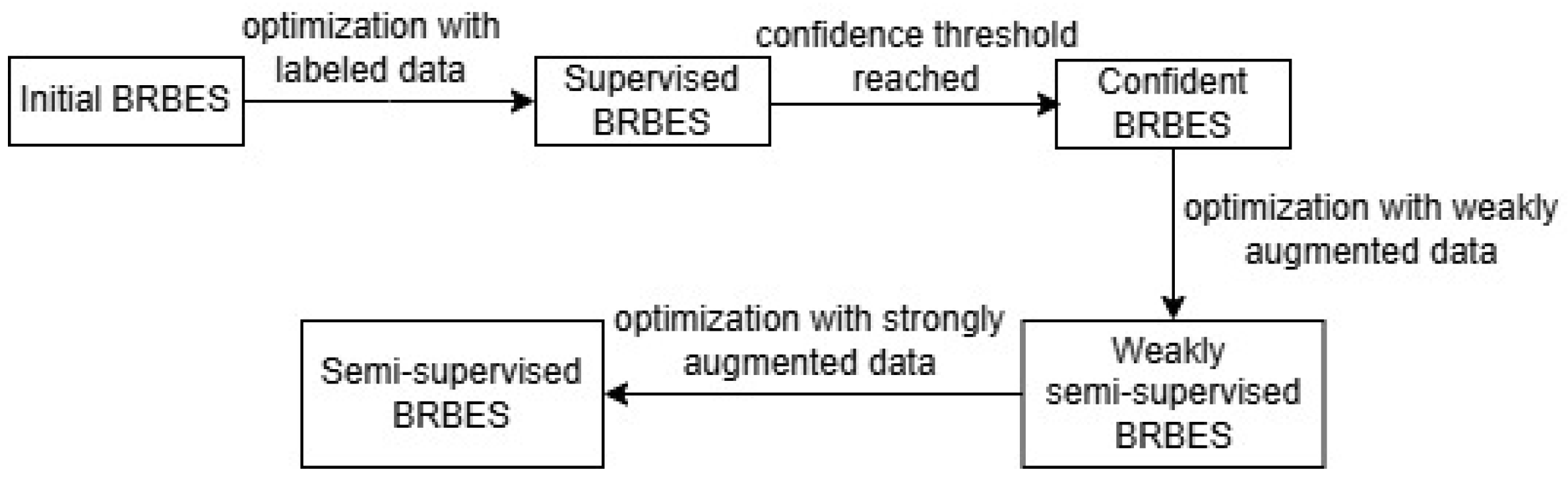
• Prediction Model: For the prediction model, we use the BRBES, a symbolic AI model, to provide domain knowledge based prediction while handling associated uncertainties (Figure 1a). We then optimize the initial BRBES with supervised labeled training data using JOPS. Such optimization makes the initial BRBES supervised. We optimize the supervised BRBES unless its accuracy reaches the confidence threshold. If the accuracy reaches this threshold, the supervised BRBES will become a confident BRBES. This confident BRBES will be able to predict pseudo-labels for the unlabeled data points with due confidence. (Figure 1b).
• Data Augmentation: To overcome the shortage of labeled data, we synthetically generate unlabeled data. For this purpose, we leverage two kinds of augmentations: “weak” and “strong”. Theses two types of augmentations are briefly mentioned below.
      Weak Augmentation: For weak augmentation, we generate unlabeled integer values for relevant antecedent attributes of BRBES. We predict labels for these weakly augmented unlabeled data points with confident BRBES. We then train the confident BRBES with both labeled and weakly augmented pseudo-labeled datasets. If training with this weakly augmented pseudo-labeled dataset improves the accuracy, the confident BRBES will transition to a weakly semi-supervised BRBES (Figure 1c–g).
      Strong Augmentation: A dataset has two types of noise: class noise and attribute noise [61]. Class noise is triggered against incorrectly assigned class label to a data instance. On the other hand, attribute noise reflects erroneous or missing values for one or more input features (independent variables) of the dataset [61]. To reduce both the class and attribute noise of the weakly augmented pseudo-labeled dataset, we apply strong augmentation. For strong augmentation, we synthetically generate unlabeled float values for the same antecedent attributes of BRBES as weak augmentation. We then predict labels for these strongly augmented unlabeled data points with a weakly semi-supervised BRBES. We optimize the weakly semi-supervised BRBES with labeled, as well as weakly and strongly augmented pseudo-labeled, datasets. If training with the strongly augmented pseudo-labeled dataset improves the accuracy, weakly semi-supervised BRBES will transition to a semi-supervised BRBES (Figure 1h–l).
• Prediction and Explanation: This semi-supervised BRBES provides more accurate prediction, along with an explanation and counterfactual, through a user interface (Figure 1m,n).

3.2. Proposed Semi-Supervised Explainable BRBES Framework

Initial Facts: The architectural design of the proposed semi-supervised explainable BRBES framework for predicting energy consumption in buildings is shown in Figure 1. Figure 1a represents the BRBES as symbolic AI which has five input values: interior space, month, day, hour, and heating method. The unit of interior space is the square meter, the month range is from January to December, the day range is from Monday to Sunday, the hour range is from 00:00 to 23:00, and heating method is either district or electric. These five values constitute five initial facts for the BRBES to provide energy consumption prediction. Among these facts, month, day, and hour are used to calculate solar illumination and interior inhabitance level of a building at a specific time instance. Against these initial facts, the BRBES predicts the energy consumption level in kWh by reasoning over its rule base. We now proceed to illustrate how this rule base of the BRBES models energy consumption knowledge to deliver transparent and explainable prediction.

Formalization of Domain Knowledge: The body of knowledge that individuals have acquired in a particular area of expertise is called domain knowledge [62]. It can be viewed as a specialized manifestation of prior knowledge held by a domain expert or individual [63]. Knowledge of the energy consumption domain is represented by the rule base of the BRBES. Here, energy consumption serves as the domain of interest, and the rule base embodies the corresponding domain knowledge. A belief rule consists of two components: an antecedent part and a consequent part. In the rule base of the BRBES within our proposed semi-supervised framework, the antecedent part comprises three attributes: interior space, solar illumination, and interior inhabitance. The solar illumination value, ranging from 0 to 1, is derived based on the month and hour, as illustrated in

Table 2. Solar illumination calculation from January to December.

Independent Variables		Outcome
Period	Time	Solar Illumination (%)
January	9:00 a.m. to 2:00 p.m. 2:01 p.m. to 4:00 p.m. 7:00 a.m. to 8:59 a.m. rest of the day	100 50 50 0
February	8:00 a.m. to 4:00 p.m. 4:01 p.m. to 6:00 p.m. 6:00 a.m. to 7:59 a.m. rest of the day	100 50 50 0
March	6:00 a.m. to 5:00 p.m. 5:01 p.m. to 7:00 p.m. 4:00 a.m. to 5:59 a.m. rest of the day	100 50 50 0
April	4:00 a.m. to 7:00 p.m. 7:01 p.m. to 9:00 p.m. 2:00 a.m. to 3:59 a.m. rest of the day	100 50 50 0
May	2:00 a.m. to 9:00 p.m. 9:01 p.m. to 11:00 p.m. 00:00 to 1:59 a.m. rest of the day	100 50 50 0
June	1:00 a.m. to 10:00 p.m. rest of the day	100 50
July	2:00 a.m. to 10:00 p.m. rest of the day	100 50
August	4:00 a.m. to 8:00 p.m. 8:01 p.m. to 10:00 p.m. 2:00 a.m. to 3:59 a.m. rest of the day	100 50 50 0
September	5:00 a.m. to 6:00 p.m. 6:01 p.m. to 8:00 p.m. 3:00 a.m. to 4:59 a.m. rest of the day	100 50 50 0
October	7:00 a.m. to 4:00 p.m. 4:01 p.m. to 6:00 p.m. 5:00 a.m. to 6:59 a.m. rest of the day	100 50 50 0
November	8:00 a.m. to 2:00 p.m. 2:01 p.m. to 4:00 p.m. 6:00 a.m. to 7:59 a.m. rest of the day	100 50 50 0
December	10:00 a.m. to 1:00 p.m. 1:01 p.m. to 3:00 p.m. 8:00 a.m. to 9:59 a.m. rest of the day	100 50 50 0

. Sunrise and sunset times are utilized to determine the corresponding solar illumination level.

Table 3. Interior inhabitance computation (weekdays).

Days	Period	Time	Interior Inhabitance (%)
Monday to Friday	September to May	8:00 a.m. to 7:00 p.m.	50
		7:01 p.m. to 10:00 p.m. (Friday)	50
		7:01 p.m. to 10:00 p.m. (Monday–Thursday)	80
		rest of the day	100
	June to August	8:00 a.m. to 7:00 p.m.	30
		7:01 p.m. to 11:00 p.m. (Friday)	50
		7:01 p.m. to 11:00 p.m. (Monday–Thursday)	70
		rest of the day	80

and

Table 4. Interior inhabitance computation (weekend).

Days	Period	Time	Interior Inhabitance (%)
Saturday–Sunday	September to May	9:00 a.m. to 7:00 p.m.	40
		7:01 p.m. to 10:00 p.m. (Sun)	80
		7:01 p.m. to 10:00 p.m. (Sat)	50
		rest of the day	80
	June to August	9:00 a.m. to 7:00 p.m.	10
		7:01 p.m. to 11:00 p.m. (Sun)	50
		7:01 p.m. to 11:00 p.m. (Sat)	30
		rest of the day	50

present the calculation of interior inhabitance (ranging from 0 to 1) in an apartment, in line with the hour of the day, month of the year, and category of the day (weekday/weekend). Each antecedent attribute is assigned three referential values: high (H), medium (M), and low (L). The consequent attribute, Energy Consumption, shares the same referential value structure. We show the hierarchical relationship between three antecedent attributes and their consequent attributes in Figure 2. Against three referential values of each of the three antecedent attributes, the rule base of the BRBES contains twenty-seven rules. There are four ways to create this rule base [47]: transforming expert knowledge into belief rules, formulating belief rules from historical data, leveraging the existing rule base, and generating rules at random without any prior information. Drawing upon the knowledge provided by energy experts, the initial rule base of the BRBES is constructed in this article. These rules, outlined in

Table 5. BRBES’s initial rule base (knowledge of energy consumption domain).

Antecedent Part				Consequent Part			Activation Weight
Rule No.	Interior Space	Solar Illumination	Interior Inhabitance	Energy Consumption
				H (%)	M (%)	L (%)
1	High	High	High	60	40	0	0
2	High	High	Medium	40	60	0	0
3	High	High	Low	0	80	20	0.49
4	High	Medium	High	80	20	0	0
5	High	Medium	Medium	60	40	0	0
6	High	Medium	Low	40	60	0	0
7	High	Low	High	100	0	0	0
8	High	Low	Medium	80	20	0	0
9	High	Low	Low	60	40	0	0
10	Medium	High	High	20	80	0	0
11	Medium	High	Medium	0	20	80	0
12	Medium	High	Low	0	60	40	0.51
13	Medium	Medium	High	20	80	0	0
14	Medium	Medium	Medium	0	100	0	0
15	Medium	Medium	Low	0	80	20	0
16	Medium	Low	High	80	20	0	0
17	Medium	Low	Medium	60	40	0	0
18	Medium	Low	Low	40	60	0	0
19	Low	High	High	0	20	80	0
20	Low	High	Medium	0	10	90	0
21	Low	High	Low	0	0	100	0
22	Low	Medium	High	0	60	40	0
23	Low	Medium	Medium	0	30	70	0
24	Low	Medium	Low	0	20	80	0
25	Low	Low	High	0	60	40	0
26	Low	Low	Medium	0	40	60	0
27	Low	Low	Low	0	20	80	0

, serve as the formal representation of the domain knowledge employed in this work. Initially, for all the rules of the rule base, we assign an equal value (“1”) to both the rule weight and antecedent attribute weight. The consequent component of the rule base contains numerical values that quantify the belief degrees for the associated referential values. The initial belief degrees allocated to these referential values of the consequent attribute of a belief rule are assigned by taking opinions of two energy experts. These belief degrees enable the BRBES to effectively handle uncertainties [47]. This table’s ‘Activation weight’ column is interpreted subsequently in this subsection.

Symbolic AI: As a symbolic AI model, we employ the BRBES in our proposed framework, as shown in Figure 1a. The reasoning mechanism of the BRBES comprises four stages: input transformation, rule activation weight calculation, belief degree update, and rule aggregation [46].

Transformation of Input. In this step, the input data corresponding to the three antecedent attributes of the rule base—interior space, solar illumination, and interior inhabitance—are transformed into their respective referential values. For interior space, the utility values for low (L), medium (M), and high (H) are set to 10, 85, and 200, respectively. For solar illumination, the L, M, and H values are 0, 0.50, and 1; and for occupancy, they are 0.10, 0.55, and 1, respectively. These utility values are initially set based on the opinions of two energy experts and two civil engineers. To illustrate our proposed framework, an apartment in Skellefteå, Sweden, is considered as a case study. This apartment has an interior space of 142 square meters and is heated with electrical technique. The goal is to predict its hourly energy consumption for 11:00 AM on a Saturday in July. The input values are converted into referential values. For interior space, M = (200 − 142)/(200 − 85) = 0.51, H = (1 − 0.51) = 0.49, and L = 0. For solar illumination, H = 1, M = (1 − 1) = 0, and L = 0. For occupancy, L = 1, M = 0, and H = 0.

Rule Activation Weight Calculation. In this step, the activation weight for each of the twenty-seven rules in the rule base is calculated. The activation weight is influenced by the input values corresponding to the three antecedent attributes. To determine the activation weight (ranging from 0 to 1) of each rule, we take into account factors such as the rule’s matching degree, rule weight, the total number of antecedent attributes, and the weight assigned to each antecedent attribute [47]. The mathematical formulations for calculating the matching degree and activation weight of each rule are provided in Equations (A1) and (A2) in Appendix A, respectively. The activation weights of the rules are presented in the last column of Table 5, where Rule No. 12 exhibits the highest activation weight of 0.51 for the given example.

Belief Degree Update. Uncertainty arising from ignorance may result in the unavailability of input data for one or more antecedent attributes. To address this issue, the BRBES updates the initial belief degrees of the referential values for its consequent attribute, as outlined in Equation (A3) of Appendix A [46]. In this manner, the BRBES effectively manages uncertainty due to ignorance.

ER-based Inference. In this step, we utilize an analytical ER approach to aggregate all twenty-seven rules of the BRBES [64,65]. The final aggregated belief degree for each of the three referential values of the consequent attribute is calculated using the analytical ER equations, as presented in Equations (A4) and (A5) of Appendix A. The resulting aggregated belief degrees for the referential values H, M, and L of the consequent attribute are 0, 0.73, and 0.27, respectively. Subsequently, the crisp value of energy consumption is determined from these three aggregated belief degrees of the consequent attribute.

Prediction of Consumed Energy. The three aggregated belief degrees of the consequent attribute in the BRBES are converted into a single numerical crisp value.

Table 6. Quantification of consumed energy in kWh using crisp value.

Belief Degrees of Consequent Attribute	Consumed Energy (District Heating)	Consumed Energy (Electric Heating)
H is the highest	(H × 2.40) + (M × 0.80)	(H × 4) + (M)/2
L is the highest	((1 − L) × 0.65) + (M × 0.15)	((1 − L) × 2) + (M × 2)/3
M is 100%	M × 0.40	M × 3
M is the highest, next is H	(M × 0.40) + (H × 2.40)/5	(M × 3) + H
M is the highest, next is L	(M × 0.40) − (L × 0.20)/5	(M × 2) − (L)/5

outlines the calculation procedure for this crisp value, which quantifies energy consumption in kWh. In addition to the belief degrees, the apartment’s heating method—either district or electric—is incorporated into the calculation. As noted by [66], electric heating typically results in higher energy consumption compared to district heating. Based on the values presented in Table 6, the final crisp value of energy consumption for the example under consideration is 1.41 kWh, which closely approximates the actual measured consumption of 1.38 kWh.

However, as a knowledge-driven approach, the BRBES tends to exhibit lower accuracy compared to machine learning and deep learning models [67]. Therefore, to enhance the accuracy of the BRBES, we focus on integrating learning-based AI techniques with the framework.

Learning AI. To improve accuracy of initial BRBES, we conducted its learning with labeled training data. As shown in Figure 1b, we performed this learning by optimizing both the parameters and structure of the BRBES. The learning parameters of BRBES include its rule weight, antecedent attribute’s weight, and consequent attribute’s belief degrees [68]. These learning parameters were initially set by a human expert, which may not be accurate for a large dataset [69]. Therefore, many optimal training techniques, such as Particle Swarm Optimization (PSO), Differential Evolution (DE), and Sequential Quadratic Programming, have been employed to facilitate the learning of BRBES parameters in order to increase the accuracy of the initial BRBES results [49,70,71]. For parameter optimization, optimal training approaches based on sequential quadratic are employed. Nevertheless, they have a tendency to become trapped in local optima. As a result, the global optima in the search space cannot be found [69]. Evolutionary algorithms like PSO, DE, Genetic Algorithm (GA), and BAT, however, have circumvented this limitation by conducting random searches from any location inside the search space. Because of the optimization strategy, DE outperforms other evolutionary algorithms to optimize BRBES parameters [72]. Two main elements of the DE are exploration and exploitation. Using the data from the search space’s current focus area, exploitation creates a new solution [73]. To stay out of local optima, exploration enlarges the search space. Finding a solution’s global optima depends heavily on two DE control parameters: crossover (CR) and mutation (F) [74]. The majority of DE research has altered CR and F values according to the objective function’s fitness values [75,76]. They did not, however, take into account the various kinds of uncertainties associated with the DE algorithm. To address these uncertainties of DE, an enhanced Belief Rule-Based adaptive Differential Evolution (eBRBaDE) algorithm has been proposed by [69]. This eBRBaDE utilizes the BRBES’s inherent uncertainty handling capacity to address the uncertainties of DE. It integrates DE with the BRBES to optimize parameters of the BRBES. eBRBaDE contains two different BRBESs, named BRBES_F and BRBES_CR, to calculate the values of F and CR, respectively. By calculating the F and CR values based on population changes and objective function’s values in each iteration, the BRBES assists in achieving the ideal balance of search space between exploration and exploitation. The new population is created by carrying out the DE mutation, crossover, and selection processes using the updated F and CR values. The individual of the new population with the highest fitness value is chosen as the best option after this process is completed and the stop requirements are satisfied. Thus, eBRBaDE provides greater accuracy than DE to produce ideal values for the learning parameters of the initial BRBES by striking a balance between exploration and exploitation through its uncertainty handling mechanism [69]. The initial BRBES is then updated with the optimized values of its learning parameters. The stop criterion is then examined. It will be false for the first iteration, at which point the procedure advances to the structure optimization stage. To optimize the structure of the rule base of BRBES, we selected the optimum number of referential values of its antecedent attributes through Structure Optimization based on Heuristic Strategy (SOHS) algorithm [49]. The new structure’s learning parameters are then used to optimize the parameters of BRBES. Until the structure does not change further, these iterations continue. Thus, we jointly optimize both the parameters and structure of the BRBES with the JOPS algorithm [49]. The flowchart of this joint optimization is presented in Figure 3. To determine the optimal parameters and structure of the BRBES, JOPS uses the generalization error instead of the training error [49]. A BRBES with a small training error on its training dataset may not be able to generate ideal inference output on its testing dataset due to overfitting [49]. On the other hand, the generalization capability, quantified by generalization error, is an important criterion to evaluate a prediction model’s effectiveness in delivering stable results on data not encountered during training [77,78,79]. Using the Hoeffding inequality theorem of probability theory [80], it has been demonstrated that the generalization error is a more useful criterion than the training error for identifying the ideal parameters and structure of the BRBES [49]. An upper bound on the likelihood that the sum of random variables will differ from its expected value is provided by this Hoeffding inequality theorem. Hence, the JOPS selects the BRBES with the minimum generalization error as the most optimal BRBES. THe generalization error, ge, is shown in Equation (1):

$$ge={\displaystyle \frac{{\sum }_{i=1}^T|f\left(x_i\right)-y_i|}{T}}+\sqrt{{\displaystyle \frac{(dln2-lnr){(u\left(D_N\right)-u\left(D_1\right))}^2}{2T}}}$$

(1)

Here, the predictive output of the BRBES for the i^th input data is represented by $\mathrm{f}({\mathrm{x}}_i)$, i^th input data’s actual output is ${\mathrm{y}}_i$, the total number of independent input–output data pairs (${\mathrm{x}}_i$, ${\mathrm{y}}_i$) is quantified by T, the total number of referential values of all antecedent attributes is symbolized by T, r is the probability value within the interval (0, 1], and the interval of the predictive output f(x) is within [u(${\mathrm{D}}_1$), u(${\mathrm{D}}_N$)]. We utilize labeled training dataset to optimize BRBES with JOPS. With this optimization, the initial BRBES transitions to a supervised BRBES, as shown in Equation (2):

$$BRBE{S}_{supervised}=JOPS\left(BRBE{S}_{initial}\left(il\right)\right)$$

(2)

Here, $il$ defines the initial labeled training data. In the next step, we ensure that the accuracy of this supervised BRBES reaches a certain confidence threshold.

Confident BRBES. As part of self-training-based semi-supervised regression, we generate unlabeled data through weak and strong augmentation. Unlabeled data refer to a set of antecedent attributes, where the actual value of the corresponding consequent attribute is unknown. In this research, we generate data through augmentation for the antecedent attribute “interior space” of the BRBES. These augmented data are unlabeled because the actual values of their corresponding consequent attributes (crisp value of energy consumption in kWh) are unknown. We then predict the value of energy consumption against unlabeled data of the antecedent attributes using a supervised BRBES. This predictive value of energy consumption is the pseudo-label, which we assign to the unlabeled data. However, before predicting this pseudo-label, the accuracy of the supervised BRBES has to reach the confidence threshold. Otherwise, this BRBES will not be confident enough to predict the pseudo-label with reasonable accuracy. To evaluate this confidence level of the accuracy of supervised BRBES, we use contrastive loss [81]. This contrastive loss measures how similar a predictive output is to the actual output. For the contrastive learning loss function, we use InfoNCE loss [82], as shown in Equation (3):

$$InfoNC{E}_{loss}=-{\displaystyle \frac{1}{N}}\sum _{i=1}^{N}log{\displaystyle \frac{exp\left(sim(z_i,z_i^{+})\right)}{{\displaystyle \sum _{j=1}^{N}exp\left(sim(z_i,z_j)\right)}}}$$

(3)

where $z_i$ is an anchor, which represents a labeled data point with actual output in the test dataset; $z_i^{+}$ is the predictive output that is similar (positive pair) to the anchor; $z_j$ is the predictive output that is dissimilar (negative pair) to the anchor; N is the total number of anchors in the test dataset; and the negative sign is intended to minimize the loss. $sim\left(\right)$ is the similarity function which measures similarity and dissimilarity of the anchor with positive and negative predictive output, respectively, as shown below.

$$\begin{gathered} sim(z_i,z_i^{+})=\left\{\begin{array}{cc}1\hfill & \mathrm{if}|(\mathrm{actual} \mathrm{output})-(\mathrm{predictive} \mathrm{output})|\le (\mathrm{actual} \mathrm{output})\ast 10\%\hfill \\ 0\hfill & \mathrm{otherwise}\hfill \end{array}\right. \\ sim(z_i,z_j)=\left\{\begin{array}{cc}-1\hfill & \mathrm{if}|(\mathrm{actual} \mathrm{output})-(\mathrm{predictive} \mathrm{output})|>(\mathrm{actual} \mathrm{output})\ast 10\%\hfill \\ 0\hfill & \mathrm{otherwise}\hfill \end{array}\right. \end{gathered}$$

Here, we consider 10% as the similarity threshold of the $sim\left(\right)$ function, which returns 1 for a positive pair (similarity with anchor) and −1 for a negative pair (dissimilarity with anchor). The exponential in Equation (3) keeps the similarity positive and amplifies the differences in similarity scores. The log scales the loss to ensure that the small values do not dominate the optimization process. Thus, it maximizes the probability of correctly identifying the positive pair. In

Table 7. Values of InfoNCE loss function against different levels of similarity.

Similarity	InfoNCE Loss Value
100% 90% 80% 70% 60% 50% 40% 30% 20% 10% 0%	1 0.80 0.60 0.40 0.20 0 −0.19 −0.39 −0.59 −0.79 −1

, we show different values of the InfoNCE loss function against various levels of similarity. According to this table, higher similarity results in higher value of this loss function. In our proposed framework, we take minimum 80% similarity (InfoNCE loss 0.60 or above) as the accuracy threshold, which represents the confidence level of the predictive output of the supervised BRBES. If the accuracy reaches this confidence threshold, the supervised BRBES will transition to a confident BRBES. Otherwise, we review the rule base (Table 5) of initial BRBES and optimize the initial BRBES again using Equation (2). Transition from the supervised BRBES to the confident BRBES is shown below.

$$BRBE{S}_{supervised}=\left\{\begin{array}{cc}BRBE{S}_{confident}\hfill & \mathrm{if}{(\mathrm{InfoNCE}}_{loss}\ge 0.60)\hfill \\ \mathrm{Table} 5\mathrm{and}\mathrm{Equation}\left(2\right)\hfill & \mathrm{otherwise}\hfill \end{array}\right.$$

After transitioning to the confident BRBES, our next step is to generate unlabeled data through weak augmentation and assign pseudo-labels to the unlabeled data.

Weak Augmentation. In this step, we apply weak augmentation to generate unlabeled data for the antecedent attribute “interior space” of BRBES (Figure 1c). For interior space, we generate integer values from 10 (minimum interior space) to 200 (maximum interior space), with an interval of 1. With these generated values, we cover every possible whole number between the minimum and maximum interior space. For solar illumination and interior inhabitance, we do not generate any unlabeled data through augmentation because all possible time instances and seasonal variations are covered in Table 2 (solar illumination) and Table 3 and Table 4 (interior inhabitance). Hence, for these two antecedent attributes, we generate float values from 0 to 1, as specified in Table 2 (solar illumination) and Table 3 and Table 4 (interior inhabitance). With these generated values, we formulate a weakly augmented unlabeled dataset. This dataset combines every single possible integer value of interior space with specific values of solar illumination and interior inhabitance.

Pseudo-Label for Weakly Augmented Unlabeled Data. We then employ confident BRBES to predict the value of consequent attribute ’energy consumption’ against each set of unlabeled antecedent attributes (Figure 1d,e). Thus, with these predictive values, we assign pseudo-labels, $p{l}_w$, to the weakly augmented unlabeled dataset (Figure 1f). We mathematically show this process in Equation (4):

$$p{l}_w=BRBE{S}_{confident}(f{a}_{wu},d{l}_u,i{o}_u)$$

(4)

$$where\left\{\begin{array}{cc}f{a}_{wu}=10+(u-1)·1,\hfill & \mathrm{for}\mathrm{u}\in \mathbb{Z},1\le \mathrm{u}\le 191\hfill \\ 0\le d{l}_u\le 1\hfill & \mathrm{Table} 2\hfill \\ 0\le i{o}_u\le 1\hfill & \mathrm{Tables} 3 \mathrm{and} 4\hfill \end{array}\right.$$

Here, $f{a}_{wu}$ defines the weakly augmented unlabeled integer values for interior space. $d{l}_u$ and $i{o}_u$ refer to the unlabeled data for solar illumination and interior inhabitance, respectively.

Weakly semi-supervised BRBES. In this step, we optimize the confident BRBES with both initial labeled dataset and weakly augmented pseudo-labeled dataset using JOPS (Figure 1g). Then, we evaluate whether this pseudo-labeled dataset improves the accuracy of the confident BRBES. This accuracy is evaluated in terms of the InfoNCE loss value using the labeled test dataset. If the accuracy is the same or higher, we include this weakly augmented pseudo-labeled dataset in the training dataset of the BRBES. Thus, with increased accuracy from the weakly augmented pseudo-labeled dataset, we turn our confident BRBES into a weakly semi-supervised one (Figure 1i). In case the accuracy of the confident BRBES is reduced due to the weakly augmented pseudo-labeled dataset, we ignore this pseudo-labeled dataset. We then review the initial rule base (Table 5) of the BRBES to check for possible misrepresentation of the domain knowledge, which might have reduced the accuracy of the pseudo-labels. After fixing this misrepresentation, we go back to Equation (2) for optimizing the BRBES with initial labeled training data. We show this transition from confident BRBES to weakly semi-supervised BRBES in Equation (5):

$$BRBE{S}_{confident}=\left\{\begin{array}{cc}BRBE{S}_{wss}\hfill & \mathrm{if}({\mathrm{InfoNCE}}_{loss}\left(\mathrm{W}\right)\ge {\mathrm{InfoNCE}}_{loss}\left(\mathrm{C}\right))\hfill \\ \mathrm{Table} 5 \mathrm{and} \mathrm{Equation} \left(2\right)\hfill & \mathrm{otherwise}\hfill \end{array}\right.$$

(5)

$$where\left\{\begin{array}{c}W=JOPS\left(BRBE{S}_{confident}(il+wp)\right)\hfill \\ C=JOPS\left(BRBE{S}_{confident}\left(il\right)\right)\hfill \end{array}\right.$$

Here, $BRBE{S}_{wss}$ is the weakly semi-supervised BRBES, $il$ defines the initial labeled training data, and $wp$ defines the weakly augmented pseudo-labeled data.

The predictive accuracy can be greatly impacted by the presence of noisy data in a dataset [61]. Noise present in datasets has been empirically demonstrated to significantly deteriorate model accuracy [61]. Therefore, addressing noise in a dataset is of paramount importance for improved prediction accuracy. Two types of noise are present in a dataset: class noise and attribute noise [61]. Class noise represents an incorrectly assigned class to a data point. Class noise can be from contradictory instances (same data instances with different class labels) or mislabeled instances (instances labeled with wrong class labels). On the other hand, attribute noise reflects erroneous values for one or more input features (independent variables) of the dataset [61]. There are three different kinds of attribute noise: erroneous attribute values, missing or do not know values, and incomplete or do not care values [83]. To reduce both the class noise and attribute noise of the weakly augmented pseudo-labeled dataset $wp$, we perform strong augmentation. Such strong augmentation is intended to make this pseudo-labeled dataset more robust.

Strong Augmentation. In this stage, we perform strong augmentation by generating float values for the antecedent attribute “interior space” of the BRBES (Figure 1h). These float values range from 10.00 (minimum interior space) to 200.00 (maximum interior space), with an interval of 0.20, excluding the values of weakly augmented dataset $f{a}_{wu}$. Thus, in terms of attribute noise, these values with decimal point address the “missing or do not know values” of the antecedent attribute “interior space”. These floating-point values of the interior space are combined with specific values of solar illumination and interior inhabitance to constitute a new set of antecedent attributes. Against this set of antecedent attributes, we employ a weakly semi-supervised BRBES to predict the value of consequent attribute ’energy consumption’ (Figure 1j). Thus, with these predictive values, we assign pseudo-labels, $p{l}_s$, to the strongly augmented unlabeled dataset. We mathematically show this process in Equation (6):

$$p{l}_s=BRBE{S}_{wss}(f{a}_{su},d{l}_u,i{o}_u)$$

(6)

$$where\left\{\begin{array}{cc}f{a}_{su}=10.00+0.20k,\hfill & \mathrm{where}\mathrm{k} \in \mathbb{Z}, 0 \le \mathrm{k} \le 950,f{a}_{su} \ne f{a}_{wu}\hfill \\ 0\le d{l}_u\le 1\hfill & \mathrm{Table} 2\hfill \\ 0\le i{o}_u\le 1\hfill & \mathrm{Tables} 3 \mathrm{and} 4\hfill \end{array}\right.$$

Here, $f{a}_{su}$ is the strongly augmented unlabeled float values for interior space, and $\mathbb{Z}$ is the set of integers. In the next step, we evaluate the impact of this strongly augmented pseudo-labeled dataset to reduce the class noise of $wp$.

Semi-supervised BRBES. In this step, we append this strongly augmented pseudo-labeled dataset to the initial labeled and weakly augmented pseudo-labeled dataset. Thus, we formulate an extended dataset to cover maximum possible instances of antecedent attributes to predict energy consumption. Then, we employ the JOPS to optimize the weakly semi-supervised BRBES with this extended dataset (Figure 1k). After this optimization, if the accuracy increases or remains same, the weakly semi-supervised BRBES will transition to a semi-supervised BRBES (Figure 1l). Otherwise, we consider that the strong augmentation is noisy and go back to Equation (6) to refine the design of strong augmentation. We mathematically show this transition from weakly semi-supervised to semi-supervised BRBES in Equation (7):

$$BRBE{S}_{wss}=\left\{\begin{array}{cc}BRBE{S}_{semi-supervised}\hfill & \mathrm{if}({\mathrm{InfoNCE}}_{loss}\left(\mathrm{S}\right)\ge {\mathrm{InfoNCE}}_{loss}\left(\mathrm{W}\right))\hfill \\ \mathrm{Equation}\left(6\right)\hfill & \mathrm{otherwise}\hfill \end{array}\right.$$

(7)

$$where\left\{\begin{array}{c}S=JOPS\left(BRBE{S}_{wss}(il+wp+sp)\right)\hfill \\ W=JOPS\left(BRBE{S}_{wss}(il+wp)\right)\hfill \end{array}\right.$$

Here, $il$ is the initial labeled training data, $wp$ is the weakly augmented pseudo-labeled data, and $sp$ is the strongly augmented pseudo-labeled data. We show the step-by-step transition from initial BRBES to semi-supervised BRBES in Figure 4. Using this semi-supervised BRBES, we predict heating method based crisp value of energy consumption with improved accuracy (Figure 1m), as shown in Equation (8):

$$ec=BRBE{S}_{semi-supervised}(aa+hm)$$

(8)

Here, $ec$ is the crisp value of predictive energy consumption in kWh, $aa$ is the set of three antecedent attributes of the rule base of the BRBES, and $hm$ is the heating method of the apartment.

Explanation. To make the predictive energy consumption trustworthy, we provide explanation in support of this predictive output to the user through a user interface (Figure 1n). We provide this explanation in nontechnical human language to enable any layperson to understand it. The rule with the maximum activation weight, which is rule 12 (Table 5) in our present example at hand, serves as the foundation for this explanation. The following is our pattern to provide explanation:

“Solar illumination is [e1] in a [e2] [e3], leading to [e4] likelihood for inhabitants to remain inside on a [e5] [e3]. Therefore, because of [e6] interior space, [e1] solar illumination, [e4] interior inhabitance, and [e7] heating technique, amount of consumed energy has been predicted to be mainly [e8]”.

Here, e1 = highest activated rule’s referential value for ‘solar illumination’; e2 = season of the year, where the summer season lasts from June to August, fall lasts from September to October, winter lasts from November to March, and spring lasts from April to May; e3 = daytime. Morning is from 4:00 a.m. to 11:59 a.m., noon (midday) is at 12:00, afternoon is from 12:01 p.m. to 5:59 p.m., evening is from 6:00 p.m. to 8:00 p.m., and night is from 8:01 p.m. to 3:59 a.m.; e4 = highest activated rule’s referential value for ‘interior inhabitance’; e5 = day type. The “weekday” lasts from Monday to Thursday, the “weekend” is Saturday, and we term Friday and Sunday by themselves; e6 = highest activated rule’s referential value for ‘interior space’; e7 = heating approach based on either district or electric technique; e8 = consequent attribute’s referential value with the highest belief degree. According to this pattern, the following is the explanation of our example case’s predictive output:

“Solar illumination is high in a summer morning, leading to low likelihood for inhabitants to remain inside on a weekend morning. Therefore, because of medium interior space, high solar illumination, low interior inhabitance, and electric heating technique, amount of consumed energy has been predicted to be mainly medium”.

From this explanation, a user can comprehend the influence of pertinent factors to reach the predictive outcome of energy consumption. We also provide counterfactual in this interface to inform the user of preconditions to attain a different level of energy consumption. As shown in

Table 8. Counterfactual against the explanation.

Preconditions		Outcome
Consequent Attribute’s Highest Belief Degree	Period	Counterfactual
H	Summer	However, fewer people indoors could have resulted in decreased energy use. Furthermore, if the apartment had been heated using the district or electric approach, it might have consumed (lesser/more) energy.
	Other seasons	However, if it had been summer, when people would have been enjoying more activities outside in the solar illumination, energy consumption might have been lower. Furthermore, if the apartment had been heated using the district or electric approach, it might have consumed (lesser/more) energy.
L	Winter	However, more people indoors might have resulted in increased energy consumption. Furthermore, if the apartment had been heated using the district or electric approach, it might have consumed (lesser/more) energy.
	Other seasons	However, if it had been winter, when people would have stayed inside more often owing to the cold and lack of solar illumination, energy consumption might have been higher. Furthermore, if the apartment had been heated using the district or electric approach, it might have consumed (lesser/more) energy.
M	Winter	However, if it had been summer, when people would have been enjoying more outside activities in the solar illumination, energy consumption might have been lower. Furthermore, if the apartment had been heated using the district or electric approach, it might have consumed (lesser/more) energy.
	Other seasons	However, if it had been winter, when people would have stayed inside more often owing to the cold and lack of solar illumination, energy consumption might have been higher. Furthermore, if the apartment had been heated using the district or electric approach, it might have consumed (lesser/more) energy.

, we prepare these counterfactual statements in natural human language. Aggregated final belief degrees of all the three referential values of the consequent attribute ’energy consumption’ serve as the basis to formulate these counterfactual statements. The following is a counterfactual against the explanation of our given example:

“However, if it had been winter, when people would have stayed inside more often owing to the cold and lack of solar illumination, energy consumption might have been higher. Furthermore, if the apartment had been heated using the district approach, it might have consumed lesser energy”.

Thus, with the combination of explanation and counterfactual, we make our predictive energy consumption trustworthy to the end user. We show this semi-supervised explainable BRBES framework, denoted as $BRBE{S}_{sse}$, mathematically in Equation (9):

$$BRBE{S}_{sse}=ec+el+cf$$

(9)

Here, $ec$ is the crisp value of predictive energy consumption in kWh that we calculate in Equation (8), $el$ is the explanation text, and $cf$ is the counterfactual statement.

3.3. Framework Evaluation

We evaluated the accuracy level of our proposed semi-supervised framework with three metrics: InfoNCE loss, Mean Absolute Error (MAE), and the coefficient of determination ($R^2$). The explainability level was assessed by five metrics: feature coverage, relevance [84], test–retest reliability [85], coherence [86], and difference between explanation logic and model logic [87]. To assess the counterfactual produced by our framework, we used two metrics: pragmatism [86] and connectedness.

We used the Belief Rule-Based (BRB) adaptive Balance Determination (BRBaBD) method [37] to assess how well our proposed framework strikes a balance between explainability and accuracy. Balance is the final consequent attribute of BRBaBD, which is a multi-level BRBES. Between explainability and accuracy, the value of this balance ranges from 0 to 1, with 0 representing the least ideal point and 1 the most ideal. Its explainability level and accuracy level are its two antecedent attributes. These two antecedent attributes are each a consequent attribute of another BRBES. Five explainability metrics and three accuracy metrics formulate the antecedent attributes for explainability level and accuracy level respectively.

4. Results

4.1. Experimental Configuration

We implemented our proposed semi-supervised explainable BRBES system in Python (version 3.10) and C++ (version 20). We used a cpp file to implement the original BRBES. This cpp file also includes explanation and counterfactual statements, along with the crisp value computation dependent on the heating technique. The second cpp file was then used to implement JOPS in order to determine the ideal BRBES structure and parameter values. The first cpp file’s initial BRBES was fed these ideal values. This initial cpp file calculated the InfoNCE loss, MAE, $R^2$, coherence, the gap between explanation and model logic, and counterfactual assessment metrics (connectedness and pragmatism). We produced unlabeled data for each of the three BRBES antecedent attributes in the third cpp file.

The Python package “SHAP” was then applied to our optimized BRBES using a script written in Python. This Python script quantified three evaluation metrics: feature coverage, relevance, and test-retest reliability by calculating the SHAP value (feature importance) of each of the three antecedent properties of our rule base (Table 5). By calculating the average percentage of each antecedent attribute’s nonzero SHAP values, we determine feature coverage. We compute each antecedent attribute’s average absolute SHAP value in order to quantify relevance. By computing the Intraclass Correlation Coefficient (ICC) among the SHAP values produced by various model runs, we are able to measure test-retest reliability. This test–retest reliability was then ascertained by calculating the mean value of ICCs over many runs. In order to construct BRBaBD, we then created a fourth cpp file, entered the values of all eight evaluation metrics, and computed the balance between accuracy and explainability.

4.2. Dataset

Skellefteå Kraft of Sweden provided us with the hourly energy consumption statistics for 62 residential apartments in the city of Skellefteå in Sweden [88]. The interior space of this dataset is 58 square meters (sqm) on average, with a minimum of 23 square meters (sqm) and a high of 142 square meters (sqm). Some of these apartments run on the electric heating method and the others on the district heating method. Each of these units is 2.40 m high. Energy data from 1 January 2022 to 31 December 2022, expressed in kWh, are included in this anonymized dataset. This dataset served as our initial training dataset with labels.

This 62-apartment dataset contains hourly energy consumption value of 24 h for 365 days, which means it has total (62 × 24 × 365) = 543,120 rows. We then preprocessed this dataset by excluding the apartments with same interior space. This resulted in only 13 apartments with unique values of interior space. We replaced the missing hourly energy consumption values of these 13 apartments with mean value of previous and next hour’s energy consumption. We then combined these 13 apartments’ interior space values with three different solar illumination values (Table 2) and seven different occupancy values (Table 3 and Table 4), resulting in a dataset of (13 × 3 × 7) = 273 rows. To train and test our proposed framework, we divided these 13 apartments into two parts: 10 training apartments, and 3 testing apartments. Our weakly augmented pseudo-labeled dataset contains 191 apartments with unique interior space, resulting in (191 × 3 × 7) = 4011 rows. The strongly augmented pseudo-labeled dataset contains (951 − 191) = 760 apartments with unique interior space, resulting in (760 × 3 × 7) = 15,960 rows. Thus, our extended training dataset, consisting of labeled as well as weakly and strongly augmented pseudo-labeled data, has (10 + 191 + 760) = 961 training apartments. This means that only 1% of this extended dataset is labeled, and the remaining 99% is pseudo-labeled. We show the number of rows of the labeled, pseudo-labeled, and extended datasets in

Table 9. Labeled, pseudo-labeled, and extended datasets.

Dataset	Training	Testing
Labeled (preprocessed)	(10 × 3 × 7) = 210 rows	(3 × 3 × 7) = 63 rows
Weakly augmented pseudo-labeled data	(191 × 3 × 7) = 4011 rows	—
Strongly augmented pseudo-labeled data	(760 × 3 × 7) = 15,960 rows	—
Extended dataset (labeled + pseudo-labeled)	(210 + 4011 + 15,960) = 20,181 rows	—

. We show the histogram of number of instances across different interior space ranges in various types of dataset in Figure 5. According to Figure 5a, the data distribution in initial labeled dataset (preprocessed) is uneven, with the majority of interior space instances concentrated in the (23, 33] and (73, 83] ranges. Several intervals, such as (33, 43], (43, 53], (63, 73], (83, 93], and (103, 200] contain no instances of interior space. Such imbalance indicates potential bias in the dataset. The weakly augmented pseudo-labeled dataset (Figure 5b) shows a near-uniform distribution across all bins, suggesting an even representation of interior space values introduced through the weak augmentation. The same near-uniform distribution is visible in strongly augmented pseudo-labeled dataset (Figure 5c), with more frequent instances across interior space ranges. The extended dataset, consisting of both labeled and pseudo-labeled data (Figure 5d), shows the highest number of instances across different interior space ranges.

4.3. Results

With our proposed semi-supervised explainable BRBES framework, we performed regression instead of classification. It is not always feasible to do semi-supervised regression with the clustering assumptions used in semi-supervised classification [89]. As a result, the majority of semi-supervised classification techniques are not suitable for regression directly [89]. Due to the simplicity of data augmentation, a lot of semi-supervised learning techniques are used in language and image datasets [53]. However, our numerical energy consumption data are in tabular format, which lack context. Such a lack of context impedes augmentation due to significant information loss after augmentation [53]. Moreover, traditional data augmentation methods generate too much noise on tabular data. Therefore, due to regression on numerical tabular data, our proposed framework is not directly comparable with traditional semi-supervised learning methods, such as the consistency regularization methods, FixMatch, MixMatch, and ReMixMatch [17].

We compared our proposed semi-supervised explainable BRBES framework with four state-of-the-art semi-supervised models: Support Vector Regressor (SVR), Linear Regressor (LR), Multi-layer Perceptron (MLP) regressor, and Deep Neural Network (DNN). For the SVR, the kernel is the Radial Basis Function (RBF), the regularization parameter (c) is 100, the kernel coefficient (gamma) is 0.10, and epsilon is 0.20. For the LR, both the y intercept ($b_0$) and slope ($b_1$) are based on the least squares method. Our MLP regressor consists of two hidden layers, with six neurons per hidden layer and a dropout of 0.40. For the MLP regressor’s activation function and optimization function, we used Rectified Linear Unit (ReLU) and Stochastic Gradient Descent (SGD), respectively. For this regressor, we ran 50 epochs, with a batch size of 70, resulting in (20,181/70) = 288 iterations per epoch over the extended training dataset. For the DNN, we used eight hidden layers, each having 24 neurons. We used the same activation and optimization function as the MLP in the DNN, with a dropout of 0.50. We ran 100 epochs in the DNN, with a batch size of 70, leading to (20,181/70) = 288 iterations per epoch. Initially, we trained these four models with the labeled training dataset consisting of 10 apartments. To lessen selection bias and prediction variance, we performed five-fold crossvalidation to the original labeled dataset of 13 apartments. We then assigned pseudo-labels to the weakly and strongly augmented unlabeled dataset of 951 apartments using each of these four supervised models. These four supervised models were then retrained with extended training dataset, consisting of both labeled and concerned pseudo-labeled data. Thus, these four models transitioned from supervised to semi-supervised.

According to

Table 10. Metrics quantifying accuracy of various models.

Model	InfoNCE Loss	MAE	${\mathit{R}}^2$
Initial BRBES	0.16	0.24	0.58
Supervised BRBES	0.70	0.08	0.87
Confident BRBES	0.70	0.08	0.87
Weakly Semi-Supervised BRBES	0.76	0.05	0.89
Semi-Supervised BRBES	0.86	0.04	0.93
Support Vector Regressor (SVR) (Semi-Supervised)	0.48	0.10	0.74
Linear Regressor (LR) (Semi-Supervised)	0.32	0.18	0.66
MLP Regressor (Semi-Supervised)	0.64	0.07	0.82
Deep Neural Network (DNN) (Semi-Supervised)	0.38	0.16	0.69

, the InfoNCE loss value of the initial BRBES was only 0.16, which is very low. To improve the accuracy of the initial BRBES, we employed JOPS to optimize its parameters and structure using initial labeled data. In

Table 11. Sensitivity analysis of optimization of BRBES.

Type	Optimization	InfoNCE Loss
Parameters	P1	0.38
	P2	0.39
	P3	0.60
Structure of rule base	S1	0.39
	S2	0.56
	S3	0.45
Parameters and Structure	P1 + P2 + P3 + S2	0.70

, we analyze the sensitivity of the accuracy of BRBES to its parameters and structure [90]. We show the effect of optimizing each of the three parameters and the structure of the rule base on the accuracy of the BRBES in this table, where P1 = rule weight, P2 = each antecedent attribute’s weight, P3 = consequent attibute’s belief degrees, S1 = two referential values of each antecedent attribute, S2 = three referential values of each antecedent attribute, and S3 = four referential values of each antecedent attribute. In terms of the structure of the rule base of the BRBES, three referential values (S2) for each antecedent attribute turned out to be the most optimal one. We show this trained rule base of the BRBES with optimal belief degrees of the consequent attribute in

Table 12. BRBES’s trained rule base (after optimization).

Antecedent Part				Consequent Part
Rule No.	Interior Space	Solar Illumination	Interior Inhabitance	Energy Consumption
				H (%)	M (%)	L (%)
1	High	High	High	65	31	4
2	High	High	Medium	35	59	6
3	High	High	Low	9	80	11
4	High	Medium	High	53	26	21
5	High	Medium	Medium	71	26	3
6	High	Medium	Low	33	61	6
7	High	Low	High	69	16	15
8	High	Low	Medium	73	19	8
9	High	Low	Low	62	34	4
10	Medium	High	High	19	74	7
11	Medium	High	Medium	20	24	56
12	Medium	High	Low	3	74	23
13	Medium	Medium	High	11	84	5
14	Medium	Medium	Medium	9	86	5
15	Medium	Medium	Low	6	82	12
16	Medium	Low	High	61	31	8
17	Medium	Low	Medium	69	28	3
18	Medium	Low	Low	16	73	11
19	Low	High	High	21	28	51
20	Low	High	Medium	7	16	77
21	Low	High	Low	9	12	79
22	Low	Medium	High	4	69	27
23	Low	Medium	Medium	21	27	52
24	Low	Medium	Low	13	21	66
25	Low	Low	High	3	76	21
26	Low	Low	Medium	4	18	78
27	Low	Low	Low	3	6	91

. We then combined the optimal values of all the three parameters with the optimal structure of the BRBES using JOPS. This joint optimization resulted in a supervised BRBES with improved accuracy, as shown in Table 10. As the InfoNCE loss value of the supervised BRBES was above the confidence threshold 0.60, it became a confident BRBES. We show the comparative values of accuracy of the confident BRBES, weakly semi-supervised BRBES, semi-supervised BRBES, and four state-of-the-art semi-supervised models in Table 10. According to this table, the semi-supervised BRBES has higher accuracy than its supervised counterpart. We attribute this higher accuracy to the utilization of the pseudo-labeled training data. Moreover, this semi-supervised BRBES offers higher accuracy than four state-of-the-art semi-supervised models. Compared to SVR, LR, MLP, and DNN, the higher numbers of learning parameters of the BRBES were optimized by JOPS [68]. MLP and DNN optimized only one learning parameter—weight—using the backpropagation learning algorithm [68]. Hence, because of the optimization of a higher number of learning parameters [68], the semi-supervised BRBES offers higher accuracy than these four state-of-the-art semi-supervised models. In Figure 6, we show the increasing accuracy of the semi-supervised BRBES in terms of the InfoNCE loss value, with an increasing number of pseudo-labeled training data points. We compare the explainability metrics in

Table 13. Metrics quantifying explainability of various models.

Model	Feature Coverage	Relevance	Test-Retest Reliability	Coherence	Difference
Supervised BRBES (Nonoptimized)	1	12.01, 3.79, 5.87	146.68	87.04%	0%
Supervised BRBES (JOPS-optimized)	1	18.56, 5.15, 8.04	202.73	95.51%	0%
Weakly Semi-Supervised BRBES   (JOPS-optimized)	1	19.39, 5.36, 8.36	210.86	97.03%	0%
Semi-Supervised BRBES   (JOPS-optimized)	1	20.41, 5.62, 8.76	219.02	98.83%	0%
Support Vector Regressor (SVR)  (Semi-Supervised)	1	17.85, 4.94, 7.66	5.23	55.16%	44.18%
Linear Regressor (LR)  (Semi-Supervised)	1	16.65, 4.33, 6.57	4.44	36.77%	62.79%
MLP Regressor  (Semi-Supervised)	1	17.78, 4.91, 7.57	13.28	73.55%	25.58%
Deep Neural Network (DNN)  (Semi-Supervised)	1	17.42, 4.44, 6.66	3.46	43.67%	55.81%

.

Every model yielded 100% feature coverage against all three of the antecedent attributes of the rule base. The relevance metric represents average values of SHAP of the concerned input feature. In the third column of Table 13, we show the relevance of each of the three antecedent attributes: interior space, solar illumination, and interior inhabitance for each model. The most relevant attribute (highest SHAP value) for predicting the level of energy consumption across all models is “interior space”, which is followed by “interior inhabitance” and “solar illumination”. Compared to all other models, the semi-supervised BRBES has a higher relevance for every antecedent attribute. Furthermore, the correct formulation of the rule base and explanation interface of the semi-supervised BRBES contributed to a highly reliable test–retest, with the semi-supervised framework’s explanation having 98.83% coherence with background knowledge and an explanation fully compliant with the domain knowledge (represented by rule base) [91]. A high coherence score means that similar inputs activate similar rules of semi-supervised BRBES, indicating that the model is logically stable [92]. To evaluate the coherence of four state-of-the-art semi-supervised models, we calculated these models’ global feature importance SHAP values for each input feature across all predictions. These global feature importance values are considered as explanation of these four models. We then evaluated the coherence by measuring how consistent these SHAP value explanations are across similar inputs [84]. We calculated the difference of four state-of-the-art semi-supervised models by measuring the discrepancy (hamming difference) between feature importance SHAP values and domain knowledge (ground truth) [91]. We evaluate our semi-supervised framework’s counterfactual statements with two counterfactual metrics in

Table 14. Metrics quantifying counterfactual.

Model	Pragmatism	Connectedness
Supervised BRBES (Non-optimized)	87.50%	100%
Supervised BRBES (JOPS-optimized)	87.50%	100%
Weakly Semi-Supervised BRBES (JOPS-optimized)	87.50%	100%
Semi-Supervised BRBES (JOPS-optimized)	87.50%	100%
Support Vector Regressor (SVR) (Semi-Supervised)
Linear Regressor (LR) (Semi-Supervised)	Not applicable
MLP Regressor (Semi-Supervised)
Deep Neural Network (DNN) (Semi-Supervised)

. Our counterfactual statement’s first section addresses seasonal fluctuation, and its second section addresses the heating technique. Given that summer and winter arrive with time, the first section is entirely pragmatic. Due to the high expense of switching from electric to district heating, the second section is only partially pragmatic. Since the counterfactual is completely compatible with the BRBES’s rule base (ground truth), the connectedness is 100%. As the other four models do not generate any counterfactual, these two counterfactual metrics are irrelevant for these four models.

We used the multi-level BRBaBD to assess the model’s explainability versus accuracy balance. Using relevant evaluation metrics, we predicted the model’s explainability and accuracy values in the first layer of this BRBaBD. In Figure 7, we compare our proposed semi-supervised BRBES with four other state-of-the-art semi-supervised models in terms of explainability and accuracy values (between 0 and 1). The explainability versus accuracy balance of the semi-supervised BRBES and the other four semi-supervised state-of-the-art models were predicted in the second layer of BRBaBD. The semi-supervised BRBES exhibited greater balance than the supervised BRBES and the other four state-of-the-art semi-supervised models, as seen in Figure 8. Thus, our proposed semi-supervised framework achieves more optimal balance between explainability and accuracy by outperforming both the supervised BRBES and state-of-the-art semi-supervised models. These four state-of-the-art semi-supervised models fall under a data-driven approach [8]. These models learn representation from historical energy consumption data. They do not contain any knowledge of energy consumption domain [37]. For a biased or imbalanced dataset, the predictive output of these models will be erroneous [37]. Hence, predicting energy consumption with such models is risky in case the historical dataset is underrepresented [37]. This limitation is overcome by our proposed semi-supervised BRBES framework by providing energy prediction based on domain knowledge (ground truth).

According to Figure 7, on a scale of 0 to 1, accuracy of the semi-supervised BRBES is 0.93 against an average accuracy of 0.73 of the four state-of-the-art semi-supervised models. Hence, our semi-supervised BRBES offers (0.93 − 0.73) = 0.20 or 20% higher accuracy. We now calculate the Margin of Error (ME) [93] of this higher accuracy on 20181 instances of labeled and pseudo-labeled data using Equation (10):

$$ME=Z·\sqrt{{\displaystyle \frac{p_1(1-p_1)}{n_1}}+{\displaystyle \frac{p_2(1-p_2)}{n_2}}}$$

(10)

Here, the Z-score for 95% confidence is ≈ 1.96, and $p_1$ and $p_2$ refer to the accuracy level (between 0 and 1) of the semi-supervised BRBES and four state-of-the-art semi-supervised models, respectively. $n_1$ and $n_2$ refer to the number of data instances of the semi-supervised BRBES and four state-of-the-art semi-supervised models, respectively. For 20% higher accuracy over 20181 data instances, the ME is ±0.71%. Hence, at the 95% confidence interval, we claim that the higher accuracy of the semi-supervised BRBES lies between 19.29% and 20.71%. Similarly, Figure 7 demonstrates that the explainability of the semi-supervised BRBES is 0.98 against an average explainability of 0.69 of the four state-of-the-art semi-supervised models. Hence, our semi-supervised BRBES offers (0.98 − 0.69) = 0.29 or 29% higher explainability. With the 95% confidence interval, the ME of this higher explainability is ±0.67%. Hence, we state that the higher explainability of semi-supervised BRBES lies between 28.33% and 29.67%.

5. Discussion

Section 4.3 shows that our proposed semi-supervised BRBES framework outperforms the supervised BRBES in terms of accuracy. Weakly and strongly augmented pseudo-labeled data contribute to this improved accuracy of BRBES through evolutionary learning. We overcome the scarcity of historical labeled data with this pseudo-labeled dataset. In the future, we plan to make the BRBES self-supervised with unlabeled data. Such a self-supervised BRBES will not be dependent on any labeled data.

BRBES offers ante hoc (intrinsic) explainability through its rule base [37]. Such ante hoc explanation is faithful to the model’s actual decision-making process [94]. In legally regulated domains, users are more likely to trust ante hoc models [95]. However, ante hoc models are often task-specific, and adapting them to new domains may require redesign. On the other hand, post hoc tools explain complex models with high predictive accuracy [96]. Such post hoc techniques can be applied across various domains and architectures. However, such post hoc tools are approximations, which can lead to misleading or incomplete explanations [94]. Hence, such post hoc explanations can foster false trust, especially if users cannot assess explanation accuracy [95]. In Section 4.3 (Results), the explainability evaluation metrics demonstrate the higher explainability of ante hoc explanation of the semi-supervised BRBES than the post hoc explanation of the four state-of-the-art semi-supervised models. We provide an explanation and counterfactual of our semi-supervised framework in natural human language for improved human intelligibility. On the other hand, the post hoc explanations are provided in predefined technical format rather than human language [37]. The output of the BRBaBD confirms our framework’s high explainability and high accuracy in a balanced way.

We also plan to investigate how size of the rule base of BRBES can be reduced without compromising accuracy. Such a reduction will make the BRBES more cost-effective computationally. The runtime complexity of our proposed semi-supervised BRBES framework is $O(G·P·m^n·k)$, where G = number of generations in JOPS, P = population size in JOPS, m = number of referential values of each antecedent attribute of BRBES, n = number of antecedent attributes of the BRBES, and k = number of referential values of the consequent attribute of BRBES. Here, $m^n$ is the size of the rule base, which grows exponentially with an increasing number of n. Hence, rule base size reduction is a vital factor to improve the scalability of the BRBES. The memory requirement of the semi-supervised BRBES framework is $O(P·m^n·(k+n))$. We compare the runtime complexity and memory requirement of our proposed semi-supervised BRBES framework with the four state-of-the-art models in

Table 15. Comparative values of runtime complexity and memory requirement.

Model Remarks	Runtime Complexity	Memory Requirement
Semi-supervised BRBES	$O(G·P·m^n·k)$	$O(P·m^n·(k+n))$
Support Vector Regressor (SVR) * (Semi-Supervised)	$O\left(n^2\right)$ to $O\left(n^3\right)$	$O\left(n^2\right)$
Linear Regressor (LR) * (Semi-Supervised)	$O(k·n·d)$	$O\left(d^2\right)$
MLP Regressor * (Semi-Supervised)	$O(k·n·d·h)$	$O(d·h)$
Deep Neural Network (DNN) * (Semi-Supervised)	$O(k·n·\sum (d_l·d_{l-1}))$ (sum over layers)	$O(n_{in}·h+(L-1)·h^2$ + h · nout + L · h)

* n = number of samples, k = number of output classes, d = number of input features, h = number of neurons in a hidden layer, $d_l$, $d_{l-1}$ = layer sizes in DNN, $n_{in}$ = input size, and $n_{out}$ = output size.

[97,98]. According to this table, due to JOPS, the semi-supervised BRBES has higher runtime complexity and memory requirement than the semi-supervised SVR, LR, and MLP.

In terms of generalization, our proposed semi-supervised BRBES framework can be applied to other climates, such as, tropical, continental, or polar climates. For this purpose, solar illumination values (Table 2) and interior inhabitance values (Table 3 and Table 4) have to be updated in the context of the local climate of the region of interest. To apply this framework to other building types, such as commercial, industrial, or institutional buildings, the utility values of the referential values of the interior space and the interior inhabitance values (Table 3 and Table 4) have to be customized with respect to the concerned building(s). Moreover, an accurate rule base has to be developed with the help of relevant domain experts. Such an effective rule base will ensure high-confidence pseudo-labels for the augmented unlabeled data. To apply this framework to other domains, such as disease prediction, predictive maintenance, or stock market prediction, influential antecedent attributes have to be identified, followed by the formulation of an accurate rule base.

6. Conclusions

This research introduced a framework for predicting and explaining building energy consumption using a semi-supervised explainable Belief Rule-Based Expert System (BRBES). Knowledge of the relevant domain was utilized as the basis by the BRBES to provide this prediction while managing the uncertainties associated with data. Evolutionary learning with pseudo-labeled data made our framework semi-supervised. We examined the limitations inherent in existing semi-supervised prediction models and proposed a novel framework to effectively address these shortcomings. For the semi-supervised learning model, we used self-training to ensure domain knowledge-based prediction of the pseudo-label. The rule base of the BRBES made our framework explainable through domain knowledge. To enhance the accuracy of the BRBES, we optimized its parameters and structure with labeled data using learning AI. Once the accuracy of this optimized BRBES reached the confidence threshold, we synthetically generated unlabeled data through weak augmentation. Pseudo-labels were assigned to these unlabeled data with a confident BRBES. We optimized this confident BRBES with labeled and weakly augmented pseudo-labeled data. This optimization resulted in a weakly semi-supervised BRBES. We then synthetically generated strongly augmented unlabeled data and assigned pseudo-labels to them with a weakly semi-supervised BRBES. The weakly semi-supervised BRBES was optimized with labeled as well as weakly and strongly augmented pseudo-labeled data, resulting in a semi-supervised BRBES. The diversity and density of the unlabeled data were taken into account while applying weak and strong augmentation. To provide explanation, we took into account the highly activated rules and heating method. In order to notify the user of the prerequisites for obtaining a different outcome, we also generated counterfactuals. Explanation and counterfactual statements made our proposed framework explainable. Our proposed semi-supervised BRBES framework turned out to be better than the supervised BRBES and other state-of-the-art machine learning models to accomplish accurate prediction and explanation in a balanced manner, according to evaluation metrics’ results validated on the energy consumption dataset of Skellefteå city. The accuracy and explainability of our proposed framework can promote trust in building owners to design energy-saving strategies for their buildings based on predictive insight, thereby contributing to a sustainable energy transition in buildings. Our proposed semi-supervised framework possesses the versatility to be applied across a wide range of application domains with scarce or imbalanced historical labeled data, such as disease prediction, predictive maintenance, and stock market prediction. In summary, the insufficiency of balanced historical labeled data was addressed by this study by showcasing the effectiveness of domain knowledge-based semi-supervised learning.

Our future research direction includes a self-supervised BRBES with bi-directional explanation interface. We plan to respond to a user’s supplementary questions in human language with this bi-directional interface. Moreover, we aim to explore the long-term patterns of energy consumption in buildings in future work.

References

1. Nichols, B.G.; Kockelman, K.M. Life-cycle energy implications of different residential settings: Recognizing buildings, travel, and public infrastructure. Energy Policy 2014, 68, 232–242. [Google Scholar] [CrossRef]
2. Geng, Y.; Ji, W.; Wang, Z.; Lin, B.; Zhu, Y. A review of operating performance in green buildings: Energy use, indoor environmental quality and occupant satisfaction. Energy Build. 2019, 183, 500–514. [Google Scholar] [CrossRef]
3. Aversa, P.; Donatelli, A.; Piccoli, G.; Luprano, V.A.M. Improved Thermal Transmittance Measurement with HFM Technique on Building Envelopes in the Mediterranean Area. Sel. Sci. Pap. J. Civ. Eng. 2016, 11, 39–52. [Google Scholar] [CrossRef]
4. Cao, X.; Dai, X.; Liu, J. Building energy-consumption status worldwide and the state-of-the-art technologies for zero-energy buildings during the past decade. Energy Build. 2016, 128, 198–213. [Google Scholar] [CrossRef]
5. Pham, A.-D.; Ngo, N.-T.; Truong, T.T.H.; Huynh, N.-T.; Truong, N.-S. Predicting energy consumption in multiple buildings using machine learning for improving energy efficiency and sustainability. J. Clean. Prod. 2020, 260, 121082. [Google Scholar] [CrossRef]
6. McNeil, M.A.; Karali, N.; Letschert, V. Forecasting Indonesia’s electricity load through 2030 and peak demand reductions from appliance and lighting efficiency. Energy Sustain. Dev. 2019, 49, 65–77. [Google Scholar] [CrossRef]
7. Qiao, R.; Liu, T. Impact of building greening on building energy consumption: A quantitative computational approach. J. Clean. Prod. 2020, 246, 119020. [Google Scholar] [CrossRef]
8. Kabir, S.; Islam, R.U.; Hossain, M.S.; Andersson, K. An integrated approach of belief rule base and deep learning to predict air pollution. Sensors 2020, 20, 1956. [Google Scholar] [CrossRef]
9. Caruana, R.; Niculescu-Mizil, A. An empirical comparison of supervised learning algorithms. In Proceedings of the 23rd International Conference on Machine Learning, Pittsburgh, PA, USA, 25–29 June 2006; pp. 161–168. [Google Scholar]
10. Wei, X.; Li, Y.; Zhang, M.; Chen, Q.; Wang, H. Data-driven energy consumption prediction: Challenges and solutions. Energy Inform. 2022, 5, 18–32. [Google Scholar]
11. Sahoo, P.; Roy, I.; Ahlawat, R.; Irtiza, S.; Khan, L. Potential diagnosis of COVID-19 from chest X-ray and CT findings using semi-supervised learning. Phys. Eng. Sci. Med. 2021, 45, 31–42. [Google Scholar] [CrossRef]
12. Sahoo, P.; Roy, I.; Wang, Z.; Mi, F.; Yu, L.; Balasubramani, P.; Khan, L.; Stoddart, J.F. MultiCon: A semi-supervised approach for predicting drug function from chemical structure analysis. J. Chem. Inf. Model. 2020, 60, 5995–6006. [Google Scholar] [CrossRef]
13. Zhu, X.J. Semi-Supervised Learning Literature Survey; University of Wisconsin-Madison Department of Computer Sciences: Madison, WI, USA, 2005. [Google Scholar]
14. Chapelle, O.; Scholkopf, B.; Zien Eds, A. Semi-Supervised Learning (Chapelle, O. et al., Eds.; 2006) [Book reviews]. IEEE Trans. Neural Network 2009, 20, 542. [Google Scholar] [CrossRef]
15. Lee, D.-H. Pseudo-Label: The Simple and Efficient Semi-Supervised Learning Method for Deep Neural Networks. In Proceedings of the Workshop on Challenges in Representation Learning, ICML, Atlanta, GA, USA, 21 June 2013; Volume 2. [Google Scholar]
16. Miyato, T.; Maeda, S.; Koyama, M.; Ishii, S. Virtual Adversarial Training: A Regularization Method for Supervised and Semi-Supervised Learning. IEEE Trans. Pattern Anal. Mach. Intell. 2019, 41, 1979–1993. [Google Scholar] [CrossRef]
17. Yang, X.; Song, Z.; King, I.; Xu, Z. A survey on deep semi-supervised learning. IEEE Trans. Knowl. Data Eng. 2022, 35, 8934–8954. [Google Scholar] [CrossRef]
18. Luo, X.; Zhao, Y.; Qin, Y.; Ju, W.; Zhang, M. Towards semi-supervised universal graph classification. IEEE Trans. Knowl. Data Eng. 2023, 36, 416–428. [Google Scholar] [CrossRef]
19. Luo, X.; Zhao, Y.; Mao, Z.; Qin, Y.; Ju, W.; Zhang, M.; Sun, Y. Rignn: A rationale perspective for semi-supervised open-world graph classification. Trans. Mach. Learn. Res. 2023, 2, 1–20. [Google Scholar] [CrossRef]
20. Liu, Z.; Li, Y.; Wang, Y.; Wang, Z. Hypergraph-enhanced dual semi-supervised graph classification. In Proceedings of the AAAI Conference on Artificial Intelligence, Online, 22 February–1 March 2022; Volume 36, pp. 7603–7611. [Google Scholar]
21. Verma, V.; Kawaguchi, K.; Lamb, A.; Kannala, J.; Solin, A.; Bengio, Y.; Lopez-Paz, D. Interpolation consistency training for semi-supervised learning. Neural Netw. 2022, 145, 90–106. [Google Scholar] [CrossRef]
22. Berthelot, D.; Carlini, N.; Goodfellow, I.; Papernot, N.; Oliver, A.; Raffel, C.A. Mixmatch: A holistic approach to semi-supervised learning. Adv. Neural Inf. Process. Syst. 2019, 32, 5049–5059. [Google Scholar]
23. Berthelot, D. ReMixMatch: Semi-supervised learning with distribution matching and augmentation anchoring. In Proceedings of the International Conference on Learning Representations, Addis Ababa, Ethiopia, 30 April 2020. [Google Scholar]
24. Sohn, K.; Berthelot, D.; Carlini, N.; Zhang, Z.; Zhang, H.; Raffel, C.A.; Cubuk, E.D.; Kurakin, A.; Li, C.-L. FixMatch: Simplifying semi-supervised learning with consistency and confidence. In Proceedings of the 34th International Conference on Neural Information Processing Systems, Vancouver BC Canada, 6–12 December 2020. [Google Scholar]
25. Bai, Y.; Zhao, H.; Zhang, Y.; Liu, Y.; Xie, L. Semi-supervised Active Learning for Graph-level Classification. In Proceedings of the AAAI Conference on Artificial Intelligence, Washington, DC, USA, 7–14 February 2023; Volume 37, pp. 7520–7528. [Google Scholar]
26. Zhang, M.; Song, L.; Yang, C.; Liu, Z. Towards Effective Semi-supervised Node Classification with Hybrid Curriculum Pseudo-labeling. In Proceedings of the NeurIPS Conference, New Orleans, LA, USA, 28 November 2022; Volume 35, pp. 2175–2185. [Google Scholar] [CrossRef]
27. Liu, J.W.; Liu, Y.; Luo, X.L. Semi-supervised Learning Method. Chin. J. Comput. 2015, 38, 1592–1617. [Google Scholar]
28. Ahmad, T.; Chen, H. Empirical performance evaluation of machine learning techniques for building energy consumption forecasting. Energy Build. 2018, 165, 121–130. [Google Scholar] [CrossRef]
29. Han, S.; Han, Q.H. Review of Semi-supervised Learning Research. Comput. Eng. Appl. 2020, 56, 19–27. [Google Scholar]
30. Chen, L.; Nugent, C.D.; Wang, H. A Knowledge-Driven Approach to Activity Recognition in Smart Homes. IEEE Trans. Knowl. Data Eng. 2011, 24, 961–974. [Google Scholar] [CrossRef]
31. Bhavsar, H.; Ganatra, A. A comparative study of training algorithms for supervised machine learning. Int. J. Soft Comput. Eng. 2012, 2, 74–81. [Google Scholar]
32. Cireşan, D.C.; Meier, U.; Gambardella, L.M.; Schmidhuber, J. Deep, Big, Simple Neural Nets for Handwritten Digit Recognition. Neural Comput. 2010, 22, 3207–3220. [Google Scholar] [CrossRef]
33. Zhang, W.; Liu, F.; Wen, Y.; Nee, B. Toward explainable and interpretable building energy modelling: An explainable artificial intelligence approach. In Proceedings of the 8th ACM International Conference on Systems for Energy-Efficient Buildings, Cities, and Transportation, Coimbra, Portugal, 17–18 November 2021; pp. 255–258. [Google Scholar]
34. Zhang, Y.; Teoh, B.K.; Wu, M.; Chen, J.; Zhang, L. Data-driven estimation of building energy consumption and GHG emissions using explainable artificial intelligence. Energy 2023, 262, 125468. [Google Scholar] [CrossRef]
35. Biessmann, F.; Kamble, B.; Streblow, R. An Automated Machine Learning Approach towards Energy Saving Estimates in Public Buildings. Energies 2023, 16, 6799. [Google Scholar] [CrossRef]
36. Tsoka, T.; Ye, X.; Chen, Y.; Gong, D.; Xia, X. Explainable artificial intelligence for building energy performance certificate labelling classification. J. Clean. Prod. 2022, 355, 131626. [Google Scholar] [CrossRef]
37. Kabir, S.; Hossain, M.S.; Andersson, K. An Advanced Explainable Belief Rule-Based Framework to Predict the Energy Consumption of Buildings. Energies 2024, 17, 1797. [Google Scholar] [CrossRef]
38. Sun, R. Robust reasoning: Integrating rule-based and similarity-based reasoning. Artif. Intell. 1995, 75, 241–295. [Google Scholar] [CrossRef]
39. Buchanan, B.G.; Shortliffe, E.H. Rule Based Expert Systems: The Mycin Experiments of the Stanford Heuristic Programming Project. In The Addison-Wesley Series in Artificial Intelligence; Addison-Wesley Longman Publishing Co., Inc.: Boston, MA, USA, 1984. [Google Scholar]
40. Bourgeois, J.; Bacha, S. The fuzzy logic method to efficiently optimize electricity consumption in individual housing. Energies 2017, 10, 1701. [Google Scholar] [CrossRef]
41. Gorzałczany, M.B.; Rudziński, F. Energy Consumption Prediction in Residential Buildings—An Accurate and Interpretable Machine Learning Approach Combining Fuzzy Systems with Evolutionary Optimization. Energies 2024, 17, 3242. [Google Scholar] [CrossRef]
42. Chen, X.; Singh, M.M.; Geyer, P. Utilizing domain knowledge: Robust machine learning for building energy performance prediction with small, inconsistent datasets. Knowl.-Based Syst. 2024, 294, 111774. [Google Scholar] [CrossRef]
43. Islam, R.U.; Hossain, M.S.; Andersson, K. A novel anomaly detection algorithm for sensor data under uncertainty. Soft Comput. 2018, 22, 1623–1639. [Google Scholar] [CrossRef]
44. Pearl, J. Probabilistic Reasoning in Intelligent Systems: Networks of Plausible Inference; Morgan Kaufmann Publishers Inc.: San Francisco, CA, USA, 1988. [Google Scholar]
45. Zadeh, L.A. Fuzzy logic. Computer 1988, 21, 83–93. [Google Scholar] [CrossRef]
46. Yang, J.-B.; Liu, J.; Wang, J.; Sii, H.-S.; Wang, H.-W. Belief rule-base inference methodology using the evidential reasoning Approach-RIMER. IEEE Trans. Syst. Man Cybern. Part A Syst. Humans 2006, 36, 266–285. [Google Scholar] [CrossRef]
47. Hossain, M.S.; Rahaman, S.; Mustafa, R.; Andersson, K. A belief rule-based expert system to assess suspicion of acute coronary syndrome (ACS) under uncertainty. Soft Comput. 2018, 22, 7571–7586. [Google Scholar] [CrossRef]
48. Yang, J.-B.; Singh, M. An evidential reasoning approach for multiple-attribute decision making with uncertainty. IEEE Trans. Syst. Man Cybern. 1994, 24, 1–18. [Google Scholar] [CrossRef]
49. Yang, L.H.; Wang, Y.M.; Liu, J.; Martínez, L. A joint optimization method on parameter and structure for belief-rule-based systems. Knowl. Based Syst. 2018, 142, 220–240. [Google Scholar] [CrossRef]
50. Prakash, V.J.; Nithya, D.L. A survey on semi-supervised learning techniques. Int. J. Comput. Trends Technol. 2014, 8, 148–153. [Google Scholar] [CrossRef]
51. Hernández-García, A.; König, P. Data augmentation instead of explicit regularization. arXiv 2018, arXiv:1806.03852. [Google Scholar]
52. Kaur, P.; Khehra, B.S.; Mavi, E.B.S. Data augmentation for object detection: A review. In Proceedings of the IEEE International Midwest Symposium on Circuits and Systems (MWSCAS), Lansing, MI, USA, 9–11 August 2021; pp. 537–543. [Google Scholar]
53. Li, X.; Khan, L.; Zamani, M.; Wickramasuriya, S.; Hamlen, K.W.; Thuraisingham, B. Mcom: A semi-supervised method for imbalanced tabular security data. In Proceedings of the IFIP Annual Conference on Data and Applications Security and Privacy, Newark, NJ, USA, 18–20 July 2022; Springer International Publishing: Cham, Switzerland, 2022; pp. 48–67. [Google Scholar]
54. Silva, C.; Santos, J.S.; Wanner, E.F.; Carrano, E.G.; Takahashi, R.H. Semi-supervised training of least squares support vector machine using a multiobjective evolutionary algorithm. In Proceedings of the IEEE Congress on Evolutionary Computation, Trondheim, Norway, 18–21 May 2009; pp. 2996–3002. [Google Scholar]
55. Donyavi, Z.; Asadi, S. Diverse training dataset generation based on a multi-objective optimization for semi-supervised classification. Pattern Recognit. 2020, 108, 107543. [Google Scholar] [CrossRef]
56. Jin, H.; Li, Z.; Chen, X.; Qian, B.; Yang, B.; Yang, J. Evolutionary optimization based pseudo labeling for semi-supervised soft sensor development of industrial processes. Chem. Eng. Sci. 2021, 237, 116560. [Google Scholar] [CrossRef]
57. Gao, F.; Gao, W.; Huang, L.; Xie, J.; Gong, M. An effective knowledge transfer method based on semi-supervised learning for evolutionary optimization. Inf. Sci. 2022, 612, 1127–1144. [Google Scholar] [CrossRef]
58. Cococcioni, M.; Lazzerini, B.; Pistolesi, F. A semi-supervised learning-aided evolutionary approach to occupational safety improvement. In Proceedings of the IEEE Congress on Evolutionary Computation (CEC), Vancouver, BC, Canada, 24–29 July 2016; pp. 3695–3701. [Google Scholar]
59. Triguero, I.; García, S.; Herrera, F. Self-labeled techniques for semi-supervised learning: Taxonomy, software and empirical study. Knowl. Inf. Syst. 2015, 42, 245–284. [Google Scholar] [CrossRef]
60. Van Engelen, J.E.; Hoos, H.H. A survey on semi-supervised learning. Mach. Learn. 2020, 109, 373–440. [Google Scholar] [CrossRef]
61. Gupta, S.; Gupta, A. Dealing with noise problem in machine learning data-sets: A systematic review. In Proceedings of the fifth Information Systems International Conference, Surabaya, Indonesia, 23–24 July 2019; Volume 161, pp. 466–474. [Google Scholar]
62. Alexander, P.A.; Judy, J.E. The interaction of domain-specific and strategic knowledge in academic performance. Rev. Educ. Res. 1988, 58, 375–404. [Google Scholar] [CrossRef]
63. Alexander, P.A. Domain Knowledge: Evolving Themes and Emerging Concerns. Educ. Psychol. 1992, 27, 33–51. [Google Scholar] [CrossRef]
64. Wang, Y.M.; Yang, J.B.; Xu, D.L. Environmental impact assessment using the evidential reasoning approach. Eur. J. Oper. Res. 2006, 174, 1885–1913. [Google Scholar] [CrossRef]
65. Kabir, S.; Islam, R.U.; Hossain, M.S.; Andersson, K. An integrated approach of Belief Rule Base and Convolutional Neural Network to monitor air quality in Shanghai. Expert Syst. Appl. 2022, 206, 117905. [Google Scholar] [CrossRef]
66. Brange, L.; Englund, J.; Lauenburg, P. Prosumers in district heating networks—A Swedish case study. Appl. Energy 2016, 164, 492–500. [Google Scholar] [CrossRef]
67. Dosilovic, F.K.; Brcic, M.; Hlupic, N. Explainable artificial intelligence: A survey. In Proceedings of the IEEE 2018 41st International Convention on Information and Communication Technology, Electronics and Microelectronics (MIPRO), Opatija, Croatia, 21–25 May 2018; pp. 0210–0215. [Google Scholar]
68. Hossain, M.S.; Rahaman, S.; Kor, A.L.; Andersson, K.; Pattinson, C. A Belief Rule Based Expert System for Datacenter PUE Prediction under Uncertainty. IEEE Trans. Sustain. Comput. 2017, 2, 140–153. [Google Scholar] [CrossRef]
69. Islam, R.U.; Hossain, M.S.; Andersson, K. A learning mechanism for brbes using enhanced belief rule-based adaptive differential evolution. In Proceedings of the 2020 4th IEEE International Conference on Imaging, Vision & Pattern Recognition (icIVPR), Kitakyushu, Japan, 26–29 August 2020; pp. 1–10. [Google Scholar]
70. Yang, J.B.; Liu, J.; Xu, D.L.; Wang, J.; Wang, H. Optimization models for training belief-rule-based systems. IEEE Trans. Syst. Man Cybern.-Part A Syst. Humans 2007, 37, 569–585. [Google Scholar] [CrossRef]
71. Chang, L.; Sun, J.; Jiang, J.; Li, M. Parameter learning for the belief rule base system in the residual life probability prediction of metalized film capacitor. Knowl.-Based Syst. 2015, 73, 69–80. [Google Scholar] [CrossRef]
72. Chang, L.L.; Zhou, Z.J.; Chen, Y.W.; Liao, T.J.; Hu, Y.; Yang, L.H. Belief rule base structure and parameter joint optimization under disjunctive assumption for nonlinear complex system modeling. IEEE Trans. Syst. Man Cybern. Syst. 2018, 48, 1542–1554. [Google Scholar] [CrossRef]
73. Blum, C.; Roli, A. Metaheuristics in combinatorial optimization: Overview and conceptual comparison. ACM Comput. Surv. 2003, 35, 268–308. [Google Scholar] [CrossRef]
74. Al-Dabbagh, R.D.; Neri, F.; Idris, N.; Baba, M.S. Algorithmic design issues in adaptive differential evolution schemes: Review and taxonomy. Swarm Evol. Comput. 2018, 43, 284–311. [Google Scholar] [CrossRef]
75. Liu, J.; Lampinen, J. A fuzzy adaptive differential evolution algorithm. Soft Comput. 2005, 9, 448–462. [Google Scholar] [CrossRef]
76. Leon, M.; Xiong, N. Greedy adaptation of control parameters in differential evolution for global optimization problems. In Proceedings of the 2015 IEEE Congress on Evolutionary Computation (CEC), Sendai, Japan, 25–28 May 2015; IEEE: Piscataway, NJ, USA, 2015; pp. 385–392. [Google Scholar]
77. Barron, A.R. Approximation and estimation bounds for artificial neural networks. Mach. Learn. 1994, 14, 115–133. [Google Scholar] [CrossRef]
78. Seeger, M. PAC-Bayesian generalisation error bounds for Gaussian process classification. J. Mach. Learn. Res. 2002, 3, 233–269. [Google Scholar]
79. Vapnik, V.; Chapelle, O. Bounds on error expectation for support vector machines. Neural Comput. 2000, 12, 2013–2036. [Google Scholar] [CrossRef]
80. Hoeffding, W. Probability inequalities for sums of bounded random variables. In The Collected Works of Wassily Hoeffding; Fisher, N.I., Sen, P.K., Eds.; Springer: New York, NY, USA, 1994; pp. 409–426. [Google Scholar]
81. Zeng, Q.; Xie, Y.; Lu, Z.; Xia, Y. Pefat: Boosting semi-supervised medical image classification via pseudo-loss estimation and feature adversarial training. In Proceedings of the IEEE/CVF Conference on Computer Vision and Pattern Recognition, Vancouver, BC, Canada, 17–24 June 2023; pp. 15671–15680. [Google Scholar]
82. Oord, A.V.D.; Li, Y.; Vinyals, O. Representation learning with contrastive predictive coding. arXiv 2018, arXiv:1807.03748. [Google Scholar]
83. Zhu, X.; Xindong, W. Class noise vs. attribute noise: A quantitative study. Artif. Intell. Rev. 2004, 22, 177–210. [Google Scholar] [CrossRef]
84. Lundberg, S.M.; Lee, S.I. A unified approach to interpreting model predictions. In Proceedings of the 31st Conference on Neural Information Processing Systems (NIPS 2017), Long Beach, CA, USA, 4–9 December 2017. [Google Scholar]
85. Adebayo, J.; Gilmer, J.; Muelly, M.; Goodfellow, I.; Hardt, M.; Kim, B. Sanity checks for saliency maps. In Proceedings of the 32nd Conference on Neural Information Processing Systems (NeurIPS 2018), Montreal, QC, Canada, 2–8 December 2018. [Google Scholar]
86. Nauta, M.; Trienes, J.; Pathak, S.; Nguyen, E.; Peters, M.; Schmitt, Y.; Schlötterer, J.; van Keulen, M.; Seifert, C. From Anecdotal Evidence to Quantitative Evaluation Methods: A Systematic Review on Evaluating Explainable AI. ACM Comput. Surv. 2022, 55, 295. [Google Scholar] [CrossRef]
87. Rosenfeld, A. Better metrics for evaluating explainable artificial intelligence. In Proceedings of the 20th International Conference on Autonomous Agents and Multiagent Systems, Virtual, 3–7 May 2021; pp. 45–50. [Google Scholar]
88. Skellefteå Kraft, Sweden. Energy Consumption Dataset. 2023. Available online: https://www.skekraft.se/privat/fjarrvarme/ (accessed on 6 February 2024).
89. Xu, W.; Tang, J.; Xia, H. A review of semi-supervised learning for industrial process regression modeling. In Proceedings of the 40th IEEE Chinese Control Conference (CCC), Shanghai, China, 26–28 July 2021; pp. 1359–1364. [Google Scholar]
90. Ankenbrand, M.J.; Shainberg, L.; Hock, M.; Lohr, D.; Schreiber, L.M. Sensitivity analysis for interpretation of machine learning based segmentation models in cardiac MRI. BMC Med. Imaging 2021, 21, 27. [Google Scholar] [CrossRef] [PubMed]
91. Mitruț, O.; Moise, G.; Moldoveanu, A.; Moldoveanu, F.; Leordeanu, M.; Petrescu, L. Clarity in Complexity: How Aggregating Explanations Resolves the Disagreement Problem. Artif. Intell. Rev. 2024, 57, 338. [Google Scholar] [CrossRef]
92. Suwa, M.; Scott, A.C.; Shortliffe, E.H. An Approach to Verifying Completeness and Consistency in a Rule-Based Expert System. AI Mag. 1982, 3, 16–21. [Google Scholar]
93. Cochran, W.G. Sampling Techniques, 3rd ed.; Wiley: New York, NY, USA, 1977. [Google Scholar]
94. Lipton, Z.C. The Mythos of Model Interpretability. arXiv 2016, arXiv:1606.03490. [Google Scholar]
95. Doshi-Velez, F.; Kim, B. Towards a Rigorous Science of Interpretable Machine Learning. arXiv 2017, arXiv:1702.08608. [Google Scholar]
96. Rudin, C. Stop Explaining Black Box Machine Learning Models for High Stakes Decisions and Use Interpretable Models Instead. Nat. Mach. Intell. 2019, 1, 206–215. [Google Scholar] [CrossRef]
97. Gzar, D.A.; Mahmood, A.M.; Abbas, M.K. A Comparative Study of Regression Machine Learning Algorithms: Tradeoff Between Accuracy and Computational Complexity. Math. Model. Eng. Probl. 2022, 9, 2022. [Google Scholar] [CrossRef]
98. Sze, V.; Chen, Y.-H.; Yang, T.-J.; Emer, J.S. Efficient Processing of Deep Neural Networks: A Tutorial and Survey. Proc. IEEE 2017, 105, 2295–2329. [Google Scholar] [CrossRef]
Figure 1. System Architecture of semi-supervised explainable BRBES framework to provide energy consumption prediction.
Algorithms 18 00305 g001
Figure 2. Three antecedent attributes and one consequent attribute of BRBES.
Algorithms 18 00305 g002
Figure 3. Flowchart of joint optimization of BRBES.
Algorithms 18 00305 g003
Figure 4. Transition steps from initial to semi-supervised BRBES.
Algorithms 18 00305 g004
Figure 5. Histogram showing the number of instances against interior space intervals in (a) initial labeled dataset (preprocessed), (b) weakly augmented pseudo-labeled dataset, (c) strongly augmented pseudo-labeled dataset, and (d) labeled and pseudo-labeled dataset.
Algorithms 18 00305 g005
Figure 6. InfoNCE loss value of semi-supervised BRBES with different numbers of training data points.
Algorithms 18 00305 g006
Figure 7. Comparison between explainability and accuracy of different models.
Algorithms 18 00305 g007
Figure 8. Comparison of balance between explainability and accuracy of different models.
Algorithms 18 00305 g008