Next Article in Journal
A Semi-Supervised-Learning-Aided Explainable Belief Rule-Based Approach to Predict the Energy Consumption of Buildings
Previous Article in Journal
Forecasting the Remaining Useful Life of Lithium-Ion Batteries Using Machine Learning Models—A Web-Based Application
Previous Article in Special Issue
A Computationally Efficient Method for the Diagnosis of Defects in Rolling Bearings Based on Linear Predictive Coding
 
 
Due to scheduled maintenance work on our database systems, there may be short service disruptions on this website between 10:00 and 11:00 CEST on June 14th.
Article

Research on CNC Machine Tool Spindle Fault Diagnosis Method Based on DRSN–GCE Model

College of Mechanical and Vehicular Engineering, Changchun University, Changchun 130022, China
*
Author to whom correspondence should be addressed.
Algorithms 2025, 18(6), 304; https://doi.org/10.3390/a18060304
Submission received: 5 March 2025 / Revised: 13 May 2025 / Accepted: 16 May 2025 / Published: 23 May 2025

Abstract

:
Noises on the field can affect the electromechanical system characteristics in the bearing fault diagnostic process. This paper presents a deep learning-based fault-diagnosis model DRSN–GCE (Deep Relative Shrinkage Network with Gated Convolutions and Enhancements), which is designed to deal with noise and improve noise resistance. In the first step, the data are preprocessed by adding different noises with different ratios of signal to noise and different frequencies to the vibration signals. This simulates the field noise environments. The continuous wavelet transformation (CWT), which converts the time-series signal from one dimension to a time-frequency two-dimensional image, provides rich data input for the deep learning model. Secondly, a convolutional gated layer is added to the deep residual network (DRSN), which suppresses the noise interference. The residual connection structure has also been improved in order to improve the transfer of features. In complex signals, the Gated Convolutional Shrinkage Module is used to improve feature extraction and suppress noise. The experiments on the Case Western Reserve University bearing dataset show that the DRSN–GCE exhibits high diagnostic accuracy and strong noise immunity in various noise environments such as Gauss, Laplace, Salt-and-Pepper, and Poisson. DRSN–GCE is superior to other deep learning models in terms of noise suppression, fault detection accuracy, and rolling bearing fault diagnoses in noisy environments.

Graphical Abstract

1. Introduction

The reliability of rotating equipment and machinery is crucial to the modern industrial sector. It affects production, safety, and income [1,2]. Therefore, timely and accurate monitoring and diagnosis of rotating machinery failures is necessary [3]. Rolling bearings are a key component of rotating machines, and their failure directly affects stability and safety. Therefore, it is important to perform fault diagnosis [4].
Scholars have developed a number of fault detection methods using the traditional method by extracting manually the signal characteristics [5,6]. Although these methods are helpful, they need to extract fault features manually which is time-consuming and strongly depend on professional signal processing knowledge that leads to poor diagnostic efficiency [7]. Intelligent fault diagnosis methods that use deep learning to diagnose faults have been a growing trend with the rapid advancement of artificial intelligence, which includes Auto Encoder, AE [8], Convolutional Neural Network (CNN) [9], Deep Belief Network (DBN) [10], Recurrent Neural Network (RNN) [11], Deep Transfer Learning (DTL) [12], and so on.
The Convolutional Neural Network (CNN), one of the most representative deep-learning algorithms, is widely used for fault diagnosis due to its powerful feature mapping abilities, and automatically learns fault features [13]. The CNN model can automatically extract useful information from the samples. Convolutional Neural Networks (CNNs), usually improve the performance of a model by increasing its depth [14]. However, as the network deepens, the accuracy of the model may instead decrease due to poor parameter updating during the flow of gradients. For this reason, He et al. [15] proposed the deep residual network (ResNet) that centers on the use of residual connections in the network to avoid gradient vanishing and exploding for better parameter optimization. Recently, ResNet has been used in the field of fault detection. For example, Zhao et al. [16] used ResNet in order to combine multiple wavelet coefficients. Zhang et al. [17] developed a ResNet technique based on hybrid attention mechanisms and used it for fault diagnosis in wind turbine gearboxes. Wen et al. [18] combined ResNet with migration learning and achieved good performance. These models may have improved diagnostics to a certain extent. However, the vibration signals from real-world industrial fields (such as CNC machines, wind turbines, etc.) are usually noisy, and this can blur fault characteristics, reducing the effectiveness of the model learning features [19].
Zhao et al. [20] developed a Deep residual shrinkage network (DRSN) based on the residual network to deal with noise’s impact on fault diagnosis. The Deep Residual Shrinkage Network (DRSN), based on the residual network, introduces an attentive mechanism as well as a threshold soft function to reduce noise. The network improves feature learning under high noise levels and is also applicable to pattern recognition in various noise-containing fields. Tang et al. [21] proposed an improved Deep Residue Shrinkage Network to address the problem of signal distortion caused by noise reduction. Zhang et. al. [22] proposed an improved version of DRSN, replacing the soft threshold by a leaky one for better model performance. Zhang et al. [23] introduced spatial attention into DRSN to capture the spatial dependence of the feature maps, thus constructing a model that considers a hybrid attention mechanism with multiple channels. Lei Wang [24] et al. further optimized a bearing failure diagnosis model based upon DRSN–CW. This achieves a more efficient temporal features extraction and classification by combining a Long-Short-Term Memory Network (LSTM), and an attention mechanism.
Vibration, acoustic, temperature, and current signals [25,26] are commonly used as signal sources in engineering practice. The above methods of fault diagnosis for rolling bearings are often blended with noise, which can mask the characteristic of the signal. Noise in rolling bearings vibration signals is similar to Gauss noise [27] and non-Gauss sounds such as Laplace sound [28], Salt-and-Pepper noise [29], and Poisson noise [30].
The existing deep learning models generally take Gauss noise into account and have achieved good diagnostic performance, while other kinds of noise in the field need further systematic research. In this paper, the DRSN–GCE algorithm was developed to classify faults in rolling bearings based on various noise influences. To simulate real-world noise environments, the signal is augmented with different noise frequencies and signal-to-noise ratios. Second, the two-dimensional fault signal using the continuous wavelet transformation is converted into a one-dimensional time-frequency diagram to extract all the features containing noise. A gated convolution is then introduced to the DRSN in order to suppress the unwanted noise interference. Final results showed that this model is highly accurate in any noise environment, as it was validated using the Case Western Reserve University bearing data.

2. Methods

2.1. Continuous Wavelet Transform

The Continuous Wavelet Transform is a technique for signal processing that analyzes the frequency characteristics in signals with irregular frequencies or variable frequencies. Comparing with traditional frequency-domain methods such as the Discrete Fourier Transform (DFT), CWT provides global frequency information and localized insights by examining the signal in both time and frequency domains. This makes it particularly effective for capturing transient or short-lived signal features. The core concept of CWT involves generating a series of wavelet basis functions by scaling and translating a fundamental wavelet that is known as the “mother wavelet”. By convolving these wavelets with the input signal, CWT produces wavelet coefficients that encapsulate the signal’s characteristics across different scales (frequencies) and time intervals. The coefficients allow a detailed study of the evolution over time of the frequency content in a signal. The mathematical expression for the continuous wavelet transform is shown below:
C W T f a , b = 1 a + f t φ t b a r d
where f(t) denotes the original signal, (t) denotes the wavelet function, and a and b are the scale and position parameters, respectively. The frequency range of the wavelet function can be changed by adjusting the scale a, while the position parameter b controls the movement of the wavelet on the time axis.
In continuous wavelet transform, wavelet basis function is the basic function used to analyze the signal with localization properties in time and frequency domains. The wavelet basis function is expressed as follows:
φ a , b ( t ) = 1 a φ ( t b a )
where φ ( t ) denotes the mother wavelet, which is the basic wavelet form after scaling and panning; a is a scale parameter that controls the width and frequency of the wavelet function, while b is a panning parameter, which determines the position of the wavelet on the time axis. By adjusting these two parameters, the signal can be analyzed locally at different scales and positions to extract the time-frequency characteristics of the signal.
In the continuous wavelet transform, an appropriate wavelet basis function is essential for accurate signal features. Commonly used wavelet basis functions include the Morlet wavelet, Haar wavelet, Daubechies wavelet, and Mexican Hat wavelet. Among these, the Morlet wavelet is widely favored in bearing fault diagnosis due to its smoothness, symmetry, and effective modulation with accurate fault features in both frequency and time domains. Therefore, Morlet is chosen as the wavelet basis function in this paper, and its function expression is as follows:
φ m ( t ) = π 1 / 4 e j ω 0 t e t 2 / 2
where ω 0 is the corner frequency parameter that controls the frequency of the waveform; and j is an imaginary unit.
The signal containing noise is preprocessed by CWT to convert one-dimensional time-series signals into two-dimensional time-frequency images, which provides rich input data information for the deep learning model so that the model can better extract time-frequency features of faults and improve the accuracy of diagnosis. Since CWT is able to locally analyze the signal that contains noise, the deep learning model can still extract effective features from the time-frequency image for noise immunity and high diagnostic performance in noisy environments. For the time-frequency image provided by CWT to contain rich feature information, it enables better captured features of different types of faults and improves the generalization ability to unknown data.

2.2. Gated Convolutional Layer

Gated convolutional layers are widely used in neural networks. They consist of a convolutional and gating layer. Convolutional layers extract spatial information by using parameters like stride and padding. The gating mechanisms regulate the output from the convolutional layers which produces a gating signal through independent convolutional operations. The signal is then passed through a function of activation, usually a Sigmoid, to generate values between 0 and 1. The values of the gates determine the amount that information can flow through. The output of the convolutional layers is then weighted according to the gate signal. This effectively controls the information flow and enhances the ability of the network to focus on important features.
The convolutional layer’s core operation is to perform the convolution. This is performed in order to extract the features of the input data. Convolution is the core operation of the convolutional layer and it extracts features from the input data:
( X     W ) ( i , j ) = m n X ( i + m , j + n ) · W ( m , n )
Addition is used to add the result of the convolution operation with the bias, let the bias term be b, and the result of the convolution operation output (feature extraction result) with the bias is z. The expression is as follows:
z = ( X     W ) + b
The ReLU activation function introduces nonlinearities that enable the model to fit complex functions. The Sigmoid activation function, which compresses the input values into the range [0,1], serves as the gating signal, and is expressed as follows:
R e L U ( z ) = m a x ( 0 , z )
σ ( z ) = 1 1 + e z
The gating mechanism is implemented by performing element-wise multiplication between the ReLU output (main convolution result) and the Sigmoid output (gated convolution result).
The gated convolutional layer can apply low weights to irrelevant or unimportant information, effectively suppressing noise interference and enhancing the model’s performance in noisy data. The gating system can filter out invalid data based on the input characteristics, thereby increasing the robustness and stability of the model. In addition, the gated convolutional layer can extract more detailed feature information compared with the ordinary convolutional layer for better results in the bearing diagnosis task.

2.3. Deep Residual Shrinkage Networks

Deep Residual Shrinkage Network (DRSN) [20] is an algorithm developed on Deep Residual Network (DRN) that integrates soft threshold functions and attention mechanisms. The model automatically learns thresholds through the use of a residual sub-network that can remove noise from signals and eliminate redundant information.
The soft threshold function, also known as nonlinear signal processing, is used to reduce the noise interference on overall features. It does this by applying a threshold, then reducing to zero the part of the signal below the threshold, while retaining all the rest. Soft threshold functions are as follows:
s o f t _ t h r e s h o r d ( x , α ) = x α 0 x + α x > α x α x < α
The soft threshold is a parameter that is set to x, where x represents the input signal. The function is used primarily to reduce irrelevant information beneath the threshold while retaining significant feature signals.
The residual connections are a design for deep learning networks designed to address the gradient disappearing and explosion problems that occur during training. This is performed in order to improve training performance and efficiency.
The gated convolutional layer can apply low weights to irrelevant or unimportant information for suppressing noise interference and enhancing the model’s performance. The gating system can filter out invalid data based on the input characteristics, enhancing robustness in various environments. The gated layer of the convolutional algorithm can also extract detailed information about features compared to the convolutional method.

3. DRSN–GCE Model Construction

3.1. Gated Convolutional Residual Shrinkage Module

In this paper, we design a Gated Convolutional Residual Shrinkage Module as shown in Figure 1, which is a neural network module that incorporates gated convolution, residual connectivity, shrinkage mechanism, and pooling. The module implements residual connectivity on the main path and the jump connection path for more stable gradient transfer. The use of gated convolution and contraction layers enhances the feature extraction capability and noise suppression.
The output S of the Shrinkage operation is added to the output O 2 of the second gated convolutional layer and processed by the ReLU activation function to obtain the final residual output R, which can be expressed as follows:
R = R e L U ( S + O 2 )
The first and second gated convolution operations are denoted as follows, respectively,
O 1 = R e L U ( x     W c 1 + b c 1 ) × σ ( x     W g 1 + b g 1 )
O 2 = R e L U ( x     W c 2 + b c 2 ) × σ ( x     W g 2 + b g 2 )
The Shrinkage operation can be expressed as follows:
S = S h r i n k a g e ( O 1 )
where W c 1 , b c 1 , W g 1 , b g 1 represent the first major convolution kernel, first major convolution bias, first gated convolution kernel, and first gated convolution bias, separately. Correspondingly W c 2 , b c 2 , W g 2 , b g 2 are the second major convolution kernel, second major convolution bias, second gated convolution kernel, and second gated convolution, respectively. And O 1 and O 2 are outputs of the first gated convolution operation and the second gated convolution operation, separately, where S indicates the output after the Shrinkage operation and R expresses the output of the residual connection. Finally, the residual output R is processed through a pooling operation to obtain the final output.

3.2. DRSN–GCE Model Diagnostic Process

This paper’s model is shown as Figure 2. It has several functions, including feature extraction, sound reduction, and classification of different bearing states (e.g., normal state, damage to the rolling elements, damage to inner rings, damage on outer rings, etc.). The following is the specific workflow and function description of the model in bearing diagnosis:
The first step is data preprocessing. By converting a one-dimensional series of time data into a time-frequency two-dimensional map, CWT can improve bearing fault classification performance.
Next, feature extraction is performed by gated convolution (GatedConv2d) to suppress noise and highlight important features, where the BN layer (batch normalization) performs convolution output to stabilize the training and accelerate model convergence. ReLU activates features in a nonlinear way. The maximum pooling layer reduces the size of feature maps while retaining the most important features.
Then, four Gated Convolutional Residual Shrinkage Modules (blocks 1–4) are utilized, each of which achieves feature extraction and noise reduction through a combination of multi-layer gated convolution, batch normalization, ReLU activation function, shrinkage layer, and maximum pooling layer.
After feature extraction, the flattening layer spreads the multidimensional features into one-dimensional vectors in preparation for the fully connected layer (FC). Fully connected layers consist of two components: The first part maps flattened features into a three-dimensional space, and introduces nonlinearities, and the second part maps features to classification numbers. It outputs final classification results.
Finally, the output is transformed into a probability distribution by means of the Softmax activation function, which enables classification decisions on the data and is able to distinguish between different bearing states.

4. Results

4.1. Experimental Setup

All the programs were tested on a computer equipped with an Intel Core i7-14700KF processor running at 3.40 GHz, paired with an NVIDIA GPU GTX 4060 graphics card. The experiments were conducted using Python 3.10 and PyTorch 1.13 as deep learning frameworks. The learning rate was set at 0.001, and the batch size to 96. Adam was the algorithm used for optimization. The number of classes is the number of neurons that make up the FC layer. This corresponds to the number of faults markers. In Table 1, the model parameters are listed.

4.2. Introduction to the Experimental Dataset

In this paper, a generally recognized public bearing dataset is used for experimental analysis, which makes the proposed model instructive for fault diagnosis of rolling bearings under actual working conditions.
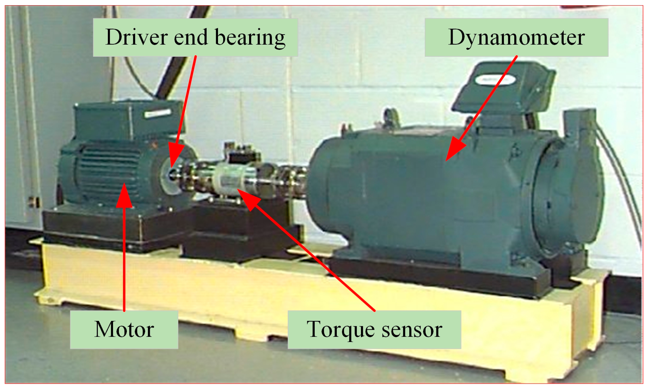
The Case Western Reserve University (CWRU) experimental setup is shown in 
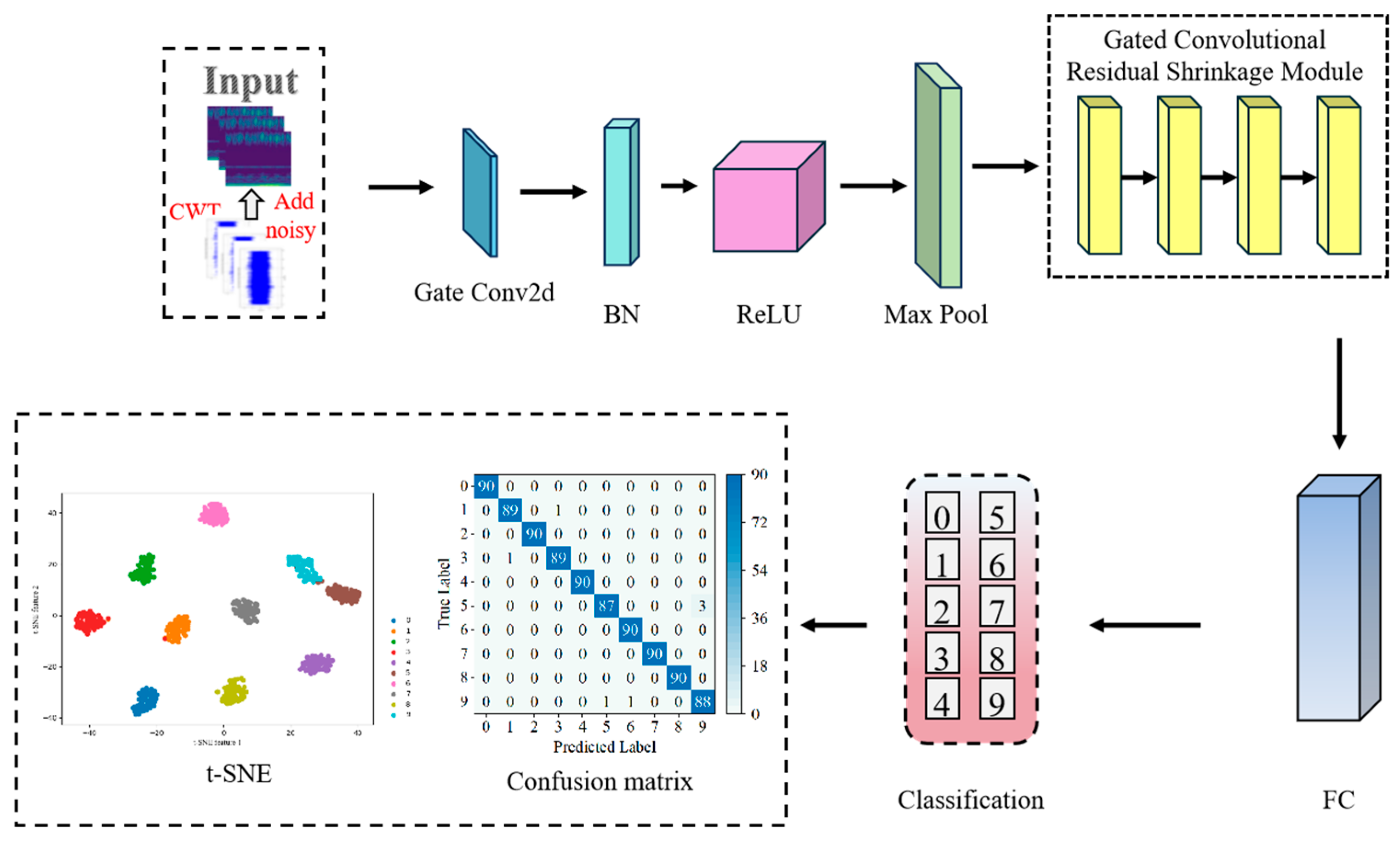
Figure 3. The experimental rig consists of a 2hp motor, dynamometer, and torque transducer. The dataset was collected using SKF6205-2RSJEM bearings at sampling frequencies of 12 kHz and 48 kHz, and a single point of failure was set up by EDM. For signal acquisition, the experimental platform was fitted with piezoelectric accelerometers (mainly PCB Piezotronics type 352C33 accelerometers), which were mounted on the drive end bearing cover (DE, Drive End) and the fan end (FE, Fan End) of the motor, and held in place by means of magnetic bases. The acquired signals were captured by a National Instruments (NI) data acquisition card and transferred to a computer for processing. The types of bearing failures include three types: rolling element failures, inner ring failures, and outer ring failures. Each failure type contains three different levels of damage diameters, and we divided the data into ten categories: one category represents normal operating conditions, and the remaining nine categories cover failure conditions. Rolling body failures with failure diameters of 0.1778 mm, 0.3556 mm, 0.5334 mm (labeled BA_I, BA_II, and BA_III, respectively), inner ring failures with failure diameters of 0.1778 mm, 0.3556 mm, 0.5334 mm (labeled IR_I, IR_II, and IR_III, respectively), and outer ring failure diameters of 0.1778 mm, 0.3556 mm, 0.5334 mm (labeled OR_I, OR_II, and OR_III, respectively) were investigated. In this study, we constructed the dataset using vibration signals from the drive-end (DE) bearings with noise artificially added to the vibration signals to simulate noise-containing signals in real industrial environments, sampled at 12 kHz with a rotational speed of 1730 rpm. Each bearing condition includes 300 samples, totaling 3000 samples, and each sample contains 2048 data points. Dividing the training set and validation set according to the ratio of 7:3, 2100 training samples and 900 validation samples can be obtained. The dataset details are shown in Table 2.
To simulate the vibrations that contain noise, we added different noise types to the vibration signals to simulate this noise. In the next experiments, we added noise to simulate the noise-containing vibration signal. Based on other research in the field of bearing diagnostics in noisy environments, we also added other non-Gauss noises to the vibration signals to make them more consistent with real industrial scenarios. For example, Lapace noise is a more complex and randomized non-Gauss noise in the real industrial scene. Salt-and-Pepper noise is also a common non-ideal noise simulation in the field of rolling bearing fault diagnosis. There is also Poisson noise, a typical non-Gauss noise. We set different signal-to-noise ratio (SNR) levels for each noise type to simulate various noise intensities, as shown in Table 3. The noise-laden vibration signals are then subjected to a continuous wavelet transform to generate a two-dimensional colored wavelet time-frequency plot, as shown in Figure 4.
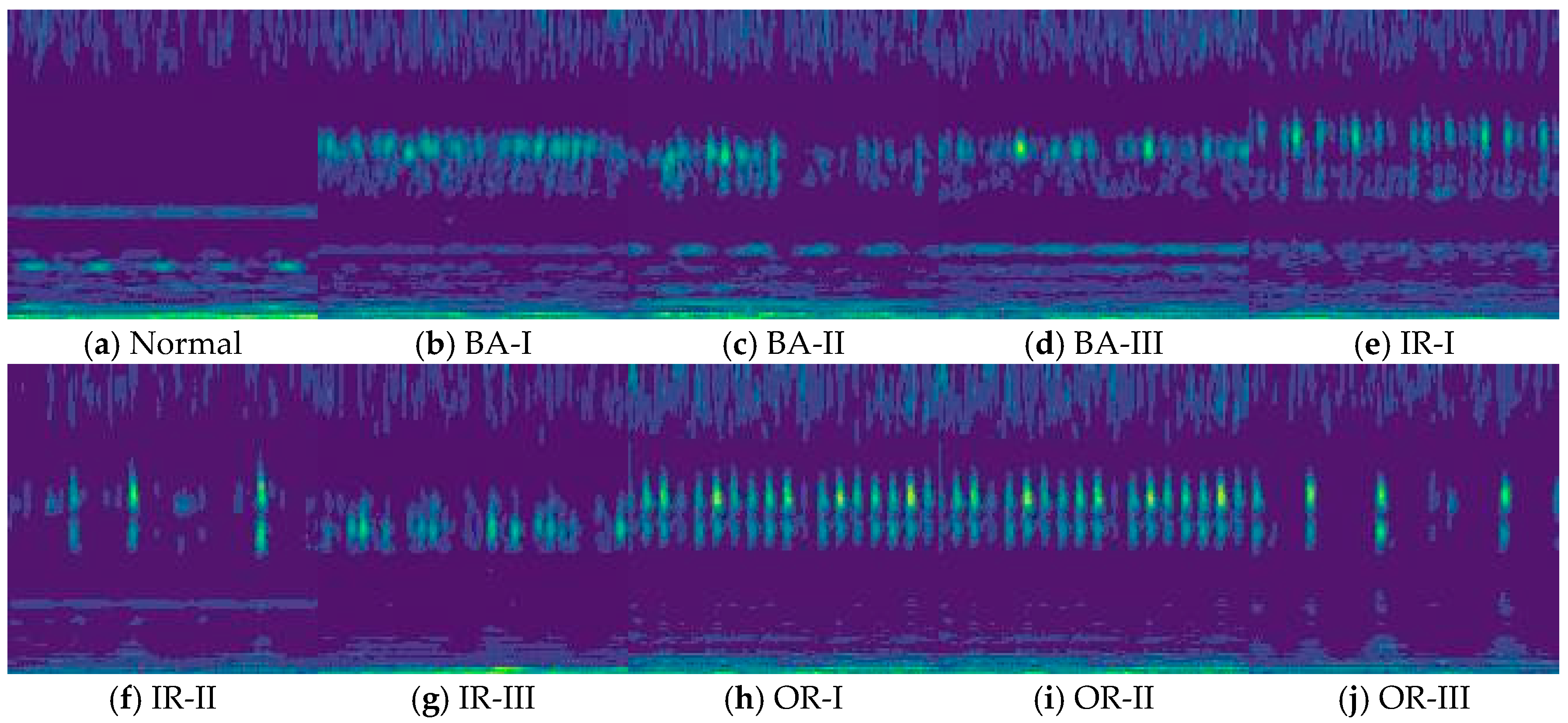
The wavelet plots of time and frequency are shown in Figure 4, for different bearings states, with a signal-to-noise ratio (SNR) of −5. In Figure 4, there is a lot of noise that has a random distribution. The noises cause confusion, blurring, and masking of local images. They also make it hard to recognize fault modes.

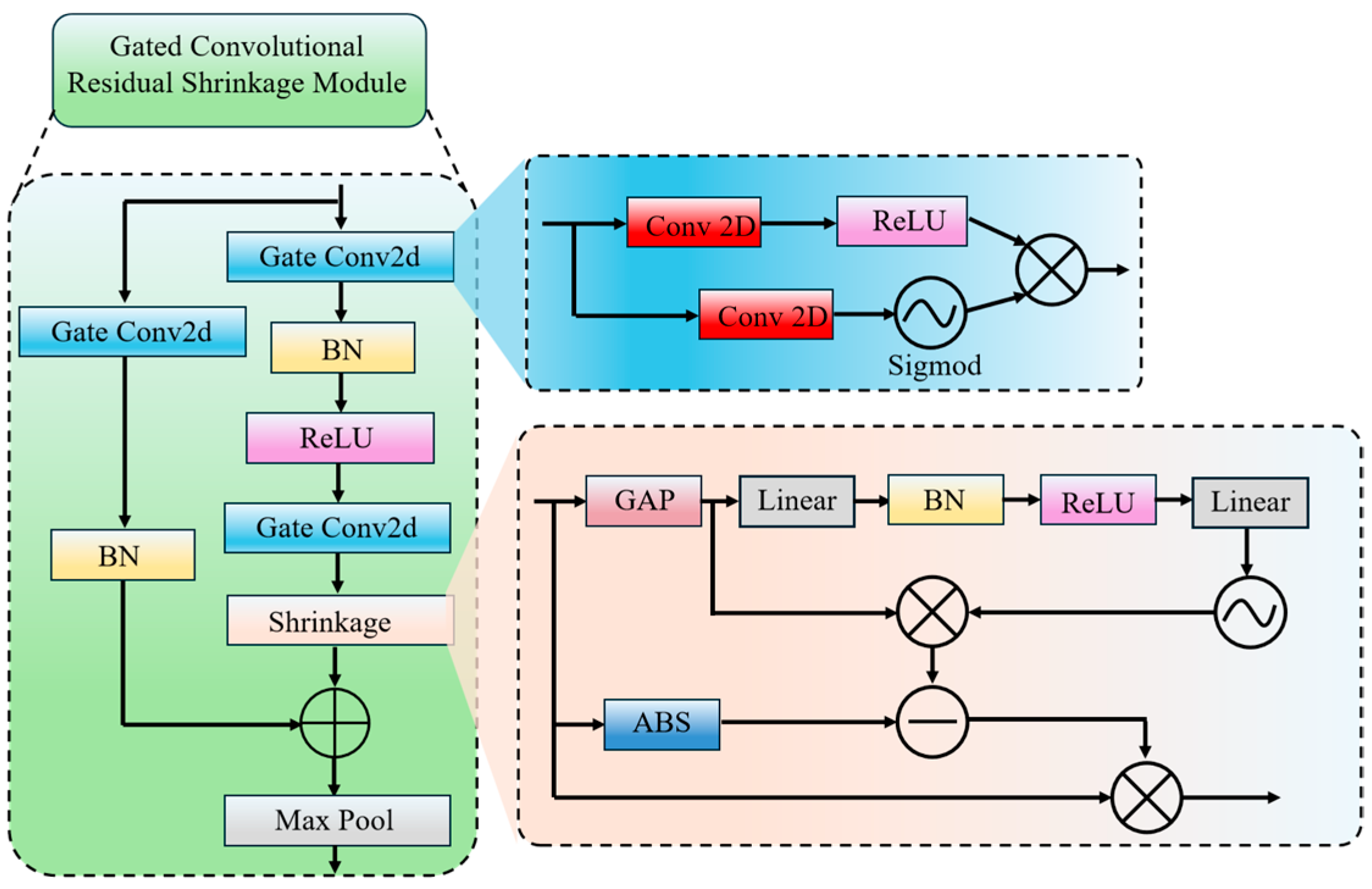
4.3. Ablation Experiment

Ablation experiments on the model are conducted to determine the efficacy of the Gated Convolutional Residual Shrinkage Module. The rolling bearing vibratory signal has a high level of intrinsic noise that is similar to Gauss. Therefore, it is chosen as an input because the signal contains the highest frequency Gauss. Method 1 used a layer of gated convolutional residual contraction module, method 2 spliced two layers, and so on incrementally, setting up six different cases through the experiment to determine the number of layers of this module spliced.
As can be seen from Table 4, Method 4 (i.e., four modules were selected for splicing) has the highest accuracy, while Methods 1, 2, and 3 have lower accuracy, and as the number of modules spliced increases (Methods 5 and 6), the accuracy decreases instead. Ablation experiments demonstrate that the design of four Convolutional Residual Gated Modules for this model is reasonable. They also show that using four module splicing balances both the complexity and ability to extract features of the model. It will not lead to low accuracy because the number of layers is too small to extract features effectively, nor will it lead to overfitting because the number of layers is too large, which affects the accuracy instead.

4.4. Comparison Test

For fault classification identification in the case of rolling bearing vibration signals affected by noise, in addition to Gauss noise, there are Laplace noise, Salt-and-Pepper noise, Poisson noise, and so on. In order to simulate the actual industrial environment, this paper introduces these noises as interferences, which are used to evaluate the robustness of the diagnostic model under various types of noise interferences.
In order to verify the effectiveness of the model in this paper, we compared it with other deep learning models (1D-CNN, CNN-Transformer, Swin Transformer, 1D-DRSN, 1DRSN–GCE). Both Gauss noise and Laplace noise (non-Gauss noise) were added to the vibration signal to obtain the mean and standard deviation of the diagnostic accuracy, precision, recall, F1 score of each batch of models with different signal-to-noise ratios. Table 5, Table 6 and Table 7 show the results. In Table 5, we can see that this model’s diagnostic accuracy is best at signal-to-noise ratios between −5 dB and 3 dB. In Table 5, we can see that this model’s diagnostic accuracy reaches 99.22% with a signal-to-noise ratio of −5. According to Table 5, the accuracy of other models is 78.81, 90.89%, 95.11%, 96.89%, and 95.44%. This paper’s diagnostic accuracy is 4.11% greater than the 1D-DRSN model, while at the same it is 3.78% more accurate than the 1DRSN–GCE model without CWT. CWT also makes it possible to better diagnose and classify the signals by converting a one-dimensional signal of time into a two-dimensional image. In Table 6, the paper’s accuracy is the best in low-frequency conditions. This shows that the model has the ability to cope with noise frequency variations. In Table 7, the performance of this model is superior to other models, in terms such as precision, recall, and F1 score.
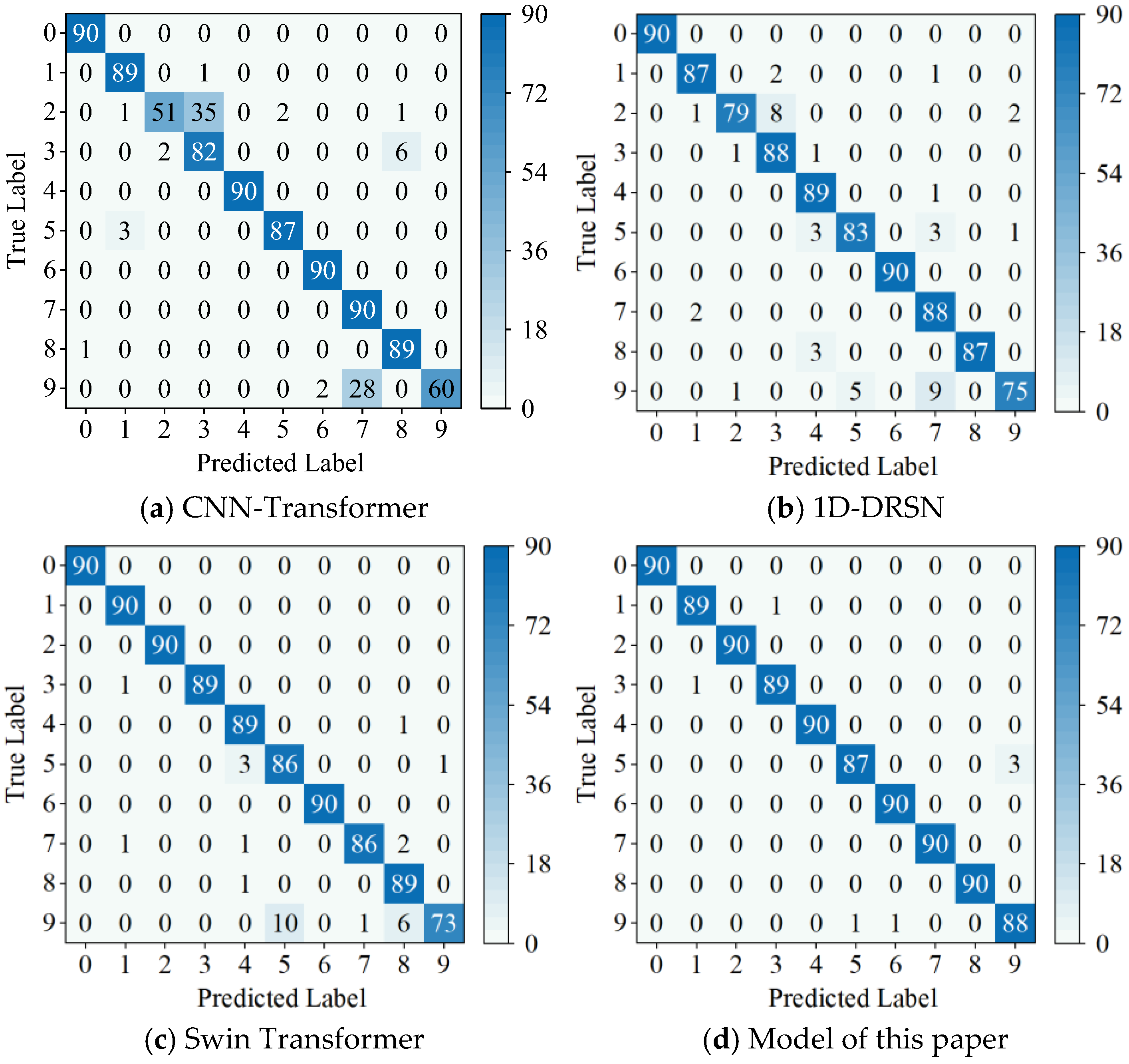
A confusion matrix was introduced to better reflect clustering of fault data and the misclassification. The confusion matrix is shown in Figure 5, which shows the results of bearing fault diagnosis using different models for high-frequency noise and a signal-to-noise ratio of −5 dB. Plot (b) of Figure 5 shows that the 1D-DRSN is able to predict faults with labels 0 and 6 perfectly, and 90 out of 100 samples have been predicted correctly. The other diagnoses, however, are incorrect to various degrees. This is especially true for marker 9 (Outer Ring Failure OR_III), as it has been misclassified by 15 of the 90 samples. The graph (d), in Figure 5, shows that the method proposed by this paper is relatively accurate at identifying these 10 types of faults. It can be observed that this method is relatively accurate in identifying these faults. At most, only three samples are incorrectly classified (Marker 5), which is the least misidentification rate. This paper shows how the method can achieve high-precision diagnosis with robustness in a noisy environment.
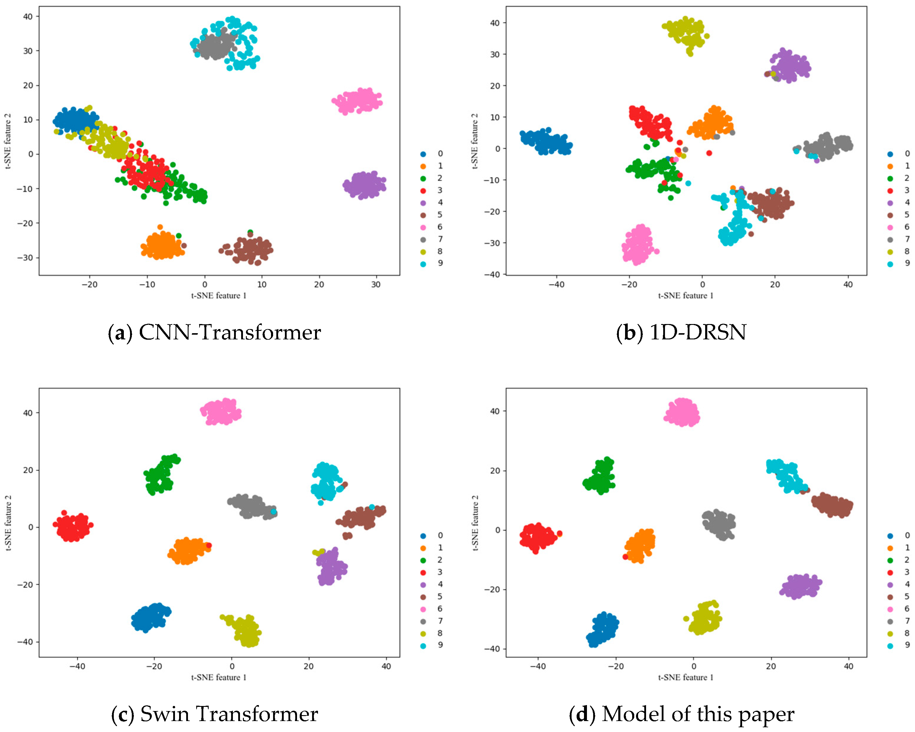
The t-SNE graph was introduced to help show fault classification more clearly. The t-SNE plots in Figure 6 show the outputs from each model with a signal-to-noise ratio of −5 dB. It is clear that this model is better than others for clustering fault features and classification of bearings.
In order to verify the effectiveness of the model in this paper, Gauss noise and non-Gauss noise (Salt-and-Pepper noise and Poisson noise) are added to the vibration signals at the same time to simulate a bearing diagnosis more consistent with a noisy environment, and again to compare the other deep learning models (1D-CNN, CNN-Transformer, Swin Transformer, 1D-DRSN, 1DRSN–GCE) to evaluate the noise immunity of other models under different noise conditions, as shown in Table 8, Table 9 and Table 10. From Table 8, it can be seen that the diagnostic accuracies of the models in this paper are the highest at signal-to-noise ratios ranging from −5 dB to 3 dB. From Table 8, it can be seen that the diagnostic accuracy of this paper’s model reaches 89.11% at a signal-to-noise ratio of −5. The other models are 76.33%, 82.01%, 85.55%, 87.00%, and 86.11% in order of accuracy from top to bottom according to Table 8. The diagnostic accuracy of this paper’s model is 3.56% higher than that of 1D-DRSN, and 3% higher than that of the 1DRSN–GCE model without CWT, which indicates that this paper’s model has good stability and noise immunity. From Table 9, it can be seen that in the low-frequency noise conditions, the accuracy of this paper’s model is also the highest in all cases, indicating that the model can cope with the frequency variation of noise. From Table 10, it can be seen that the model of this paper compared with other models in terms of precision, recall, F1 score, and so on has a more excellent performance.
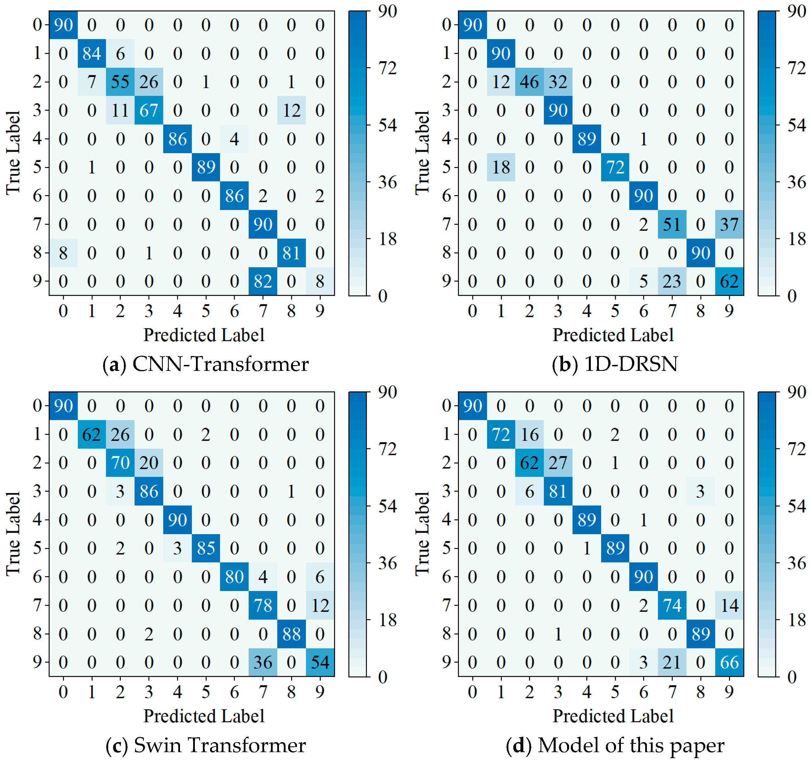
The confusion matrix in Figure 7 is a comparison of the different bearing fault diagnostic models with signal-to-noise ratios of −5 dB. The confusion matrix plot of the model in this paper has the highest accuracy, and lowest misidentification rates. This paper shows how the methods can be used to achieve high-precision diagnosis with robustness in noisy environments.
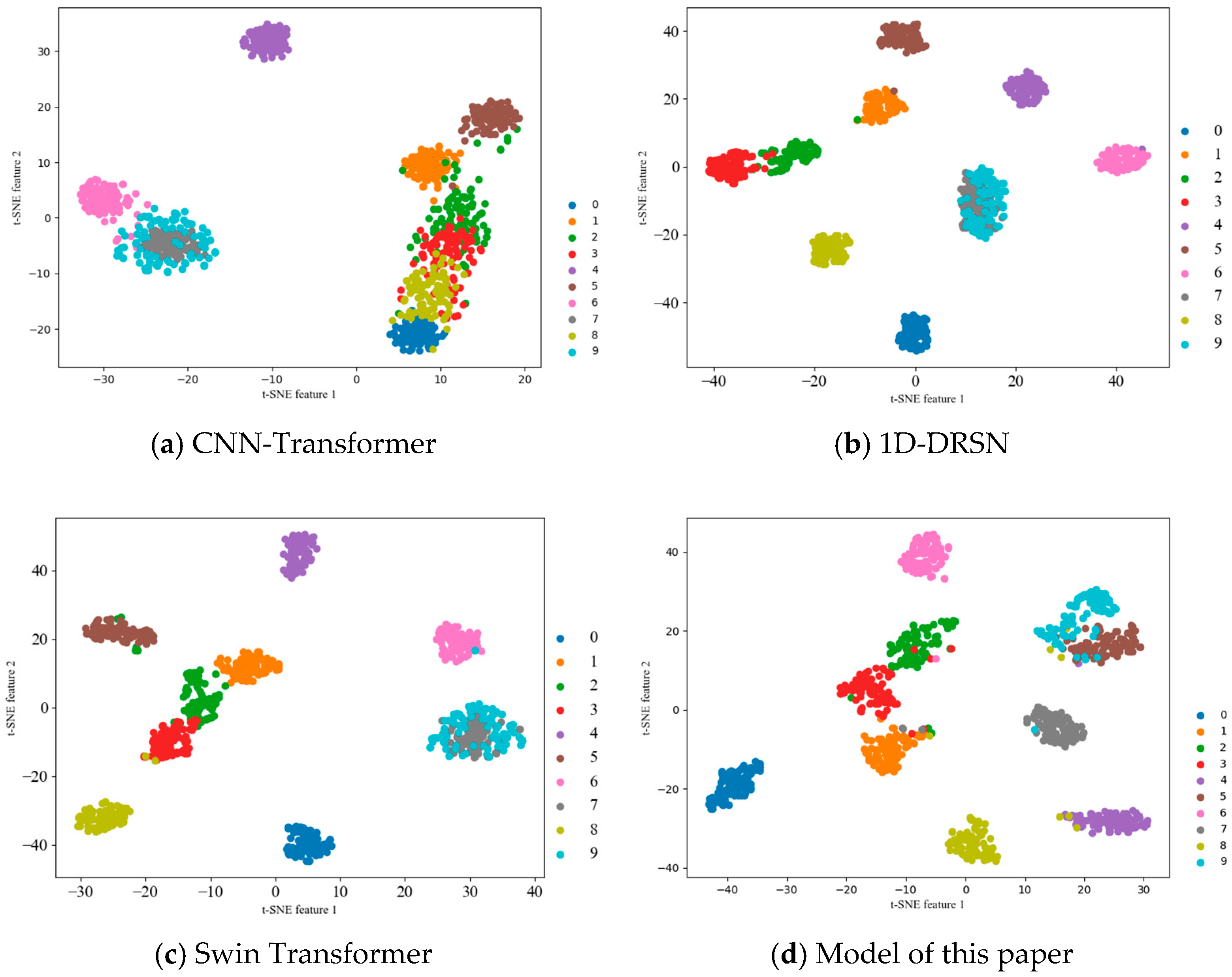
The outputs of each model are visualized using t-SNE at a signal-to-noise ratio of −5 dB. The graph (d), in Figure 8, shows that this model is superior to other deep learning models in clustering fault features and identifying bearings of different health states. It also provides a more accurate classification.

4.5. Single Noise Experiment

In the above noise experiments, we used Gauss and Laplace noise as input noises, but also added Gauss, Poisson, and Salt-and Pepper noises to the signal. These two experiments showed that adding Salt-and-Pepper noise and Poisson to the vibration signals reduced the accuracy of the models. The following experiments will be based on this model, and we will add Salt-and-Pepper noise and Poisson to the vibration signals as one input signal to investigate the impact of the two noise types on bearing fault diagnosis.
The experiment yielded Table 11, which showed that a single Salt-and-Pepper noise caused more localized damage, making it harder for the model to extract effective features. This led to relatively poor diagnostic accuracy. The model is still able to perform well despite a Salt-and-Pepper noise. Its accuracy remains over 85%. We usually believe that noise in vibration signal processing will reduce the recognition of certain features. This, in turn, affects the accuracy. However, experimental results show that the simultaneous addition of Gauss noise, Salt-and-Pepper noise, and Poisson noise to the signal, on the contrary, achieves a higher recognition accuracy than when pretzel noise is added alone. From the perspective of noise type, Salt-and-Pepper noise is a sparse discrete noise, which is mainly manifested by the abrupt change of individual points in the signal, and it is very easy to destroy the continuity and local characteristics of the signal, whereas Gauss noise is a kind of additive continuous and widely distributed random noise [31]. When these two types of noise act together on the vibration signal, a “complementary effect” is formed to some extent [32], and the Gauss noise smooths out some of the extreme pretzel points to make the signal trend more coherent, which helps the model to extract effective features. From the perspective of signal preprocessing and feature extraction, the main components of the signal after multi-noise perturbation are still preserved when it is processed by filtering (e.g., continuous wavelet transform) or feature extraction, while the Salt-and-Pepper noise may be diluted in the frequency domain, which has less impact on the fault features. As a result, the model can focus more on stable, global information rather than being misled by local noise. The introduction of multiple noises not only effectively counteracts the local destructive effect of a single noise type on model training, but also enhances the model’s ability to adapt to complex disturbed environments. This “noise against noise” strategy [33], to a certain extent, improves the accuracy of bearing fault diagnosis in the noise environment. The accuracy of this model is almost 100% in the Poisson environment. This indicates that it can deal well with vibration signals containing Poisson sound.

5. Discussion

This paper uses the DRSN–GCE model for fault diagnosis to deal with noise and its impact on bearing diagnosis. It also solves the issue of low noise resistance in the model. The specific conclusions are as follows:
(1) Continuous wavelet transform (CWT) converts the one-dimensional signal into a time-frequency two-dimensional image, providing rich data for the model. CWT is able to analyze the signals locally, but even if there are noises, the deep learning model will still be able to extract useful features. This allows the model to maintain a good diagnostic performance when in a noisy setting.
(2) The gated convolutional layer can apply low weights to irrelevant or unimportant information, effectively suppressing noise interference and improving the model’s performance in noisy data. By this method, the model can be made to show good noise immunity and fault diagnosis performance in different noise environments. Its gating mechanisms can filter out invalid data according to input characteristics, enhancing robustness in various environments.
(3) This paper proposes a structure for a Gated Convolutional Residual Shrinkage Module that can enhance the noise suppression and feature extraction abilities on complex signals. It also provides support in fault diagnosis when there are complex noise environments.
(4) The experimental results of the Case Western Reserve University bearing dataset demonstrate that the DRSN–GCE has high diagnostic accuracy and noise immunity when dealing with noisy signals like Gauss and Laplace. The model presented in this article is more noise resistant than other deep learning models. It can deal with noise impact on bearing diagnosis, and it solves the problem of model noise resistance when diagnosing bearing faults.
However, despite the superior performance of the model in different noise environments, it still has some limitations. In real industrial applications, bearing fault signals are often affected by more complex factors, such as nonlinear characteristics, multidimensional sensor data, and more diverse noise types. Further optimization of the model’s adaptability to complex noise environments is still needed in the future to support the research on rolling bearing fault diagnosis in noisy environments.

Author Contributions

Conceptualization, X.L. and J.W. (Jiahao Wang); methodology, X.L., J.W. (Jiahao Wang) and J.W. (Jixuan Wang); software, J.W. (Jiahao Wang); validation, J.W. (Jiahao Wang), J.W. (Jixuan Wang) and J.W. (Jianqiang Wang); formal analysis, J.W. (Jiahao Wang); investigation, J.W. (Jiahao Wang); resources, J.W. (Jiahao Wang); data curation, J.W. (Jiahao Wang) and J.C.; writing—original draft preparation, J.W. (Jiahao Wang); writing—review and editing, J.W. (Jiahao Wang), J.W. (Jixuan Wang), J.C. and X.Y.; visualization, J.W. (Jianqiang Wang); supervision, X.L.; project administration, X.L.; funding acquisition, X.L. All authors have read and agreed to the published version of the manuscript.

Funding

This work was supported by the Department of Education of Jilin Province under grant JJKH20251092CY, Changchun University under grant ZKP202018 and Changchun Jiamei Machinery Manufacturing Co., Ltd. under grant 2024JBH01LX6.

Data Availability Statement

The data contained in this study are available on request from the corresponding authors, except for those published. The data are not released due to confidentiality.

Conflicts of Interest

The authors declare no conflicts of interest.

References

  1. Li, W.; Zhong, X.; Shao, H.; Cai, B.; Yang, X. Multi-mode data augmentation and fault diagnosis of rotating machinery using modified ACGAN designed with new framework. Adv. Eng. Inform. 2022, 52, 101552. [Google Scholar] [CrossRef]
  2. Chen, Z.; Gryllias, K.; Li, W. Mechanical fault diagnosis using convolutional neural networks and extreme learning machine. Mech. Syst. Signal Process. 2019, 133, 106272. [Google Scholar] [CrossRef]
  3. Song, L.; Wang, H.; Chen, P. Vibration-based intelligent fault diagnosis for roller bearings in low-speed rotating machinery. IEEE Trans. Instrum. Meas. 2018, 67, 1887–1899. [Google Scholar] [CrossRef]
  4. Tian, J.; Wang, Y.J.; Wang, Z. Fault diagnosis for rolling bearing based on EEMD and spatial correlation denoising. Chin. J. Sci. Instrum. 2018, 39, 144–151. [Google Scholar]
  5. Li, Z.N.; Liu, Y.; Hu, Z.F.; Wen, C.; Wang, C.J. Empirical wavelet transform-synchroextracting transform and its applications in fault diagnosis of rolling bearing. J. Vib. Eng. 2021, 34, 1284–1292. [Google Scholar]
  6. Zhang, J.; Zhang, J.Q.; Zhong, M.; Zheng, J.D.; Li, X.K. Pso-VMD-MCKD based fault diagnosis for incipient damage in wind turbine rolling bearing. J. Vib. Meas. Diagn. 2020, 40, 287–296. [Google Scholar]
  7. Zhao, K.; Wu, S.; Li, T. A study on method of rolling bearing fault diagnosis based on Inception-BLSTM. J. Vib. Shock 2021, 40, 290–297. [Google Scholar]
  8. Sun, W.; Shao, S.; Zhao, R.; Yan, R.; Zhang, X.; Chen, X. A sparse autoencoder based deep neural network approach forinduction motor faults classification. Measurement 2016, 89, 171–178. [Google Scholar] [CrossRef]
  9. Zhou, C.; Dong, S.; Li, L. Improved convolutional neural network fault diagnosis method for rolling bearings with multi-state feature information. J. Vib. Eng. 2020, 33, 854–860. [Google Scholar]
  10. Shen, C.; Tang, S.; Jiang, X. Research on the application of independent adaptive learning rate optimized deep belief network in bearing fault diagnosis. J. Mech. Eng. 2019, 55, 81–88. [Google Scholar] [CrossRef]
  11. Chi, Y.W.; Yang, S.S.; Jiao, W.D. LSTM-RNN based multi-label classification method for rolling bearing faults. Vib. Test Diagn. 2020, 40, 563–571. [Google Scholar]
  12. Lei, Y.G.; Yang, B.; Du, Z.J.; Lu, N. Deep migration diagnosis method of mechanical equipment faults under big data. J. Mech. Eng. 2019, 55, 1–8. [Google Scholar]
  13. Eren, L.; Ince, T.; Kiranyaz, S. A generic intelligent bearing fault diagnosis system using compact adaptive 1D CNN classifier. J. Signal Process. Syst. 2019, 91, 179–189. [Google Scholar] [CrossRef]
  14. Hakim, M.; Omran, A.A.B.; Ahmed, A.N.; Al-Waily, M.; Abdellatif, A. A systematic review of rolling bearing fault diagnoses based on deep learning and transfer learning: Taxonomy, overview, application, open challenges, weaknesses and recommendations. Ain Shams Eng. J. 2023, 14, 101945. [Google Scholar] [CrossRef]
  15. He, K.; Zhang, X.; Ren, S.; Sun, J. Deep residual learning for image recognition. In Proceedings of the 2016 IEEE Conference on Computer Vision and Pattern Recognition (CVPR), Las Vegas, NV, USA, 27–30 June 2016; pp. 770–778. [Google Scholar]
  16. Zhao, M.; Kang, M.; Tang, B.; Pecht, M. Multiple wavelet coefficients fusion in deep residual networks for fault diagnosis. IEEE Trans. Ind. Electron. 2018, 66, 4696–4706. [Google Scholar] [CrossRef]
  17. Zhang, K.; Tang, B.; Deng, L.; Liu, X. A hybrid attention improved ResNet based fault diagnosis method of wind turbines gearbox. Measurement 2021, 179, 109491. [Google Scholar] [CrossRef]
  18. Wen, L.; Li, X.; Gao, L. A transfer convolutional neural network for fault diagnosis based on ResNet-50. Neural Comput. Appl. 2020, 32, 6111–6124. [Google Scholar] [CrossRef]
  19. Li, X.; Chen, J.; Wang, J.; Wang, J.; Li, X.; Kan, Y. Research on Fault Diagnosis Method of Bearings in the Spindle System for CNC Machine Tools Based on DRSN-Transformer. IEEE Access 2024, 12, 74586–74595. [Google Scholar] [CrossRef]
  20. Zhao, M.; Zhong, S.; Fu, X.; Tang, B.; Pecht, M. Deep residual shrinkage networks for fault diagnosis. IEEE Trans. Ind. Inform. 2019, 16, 4681–4690. [Google Scholar] [CrossRef]
  21. Tang, S.; Tong, J.; Zheng, K. Improved deep residual contraction network bearing fault diagnosis method. Vib. Shock 2023, 42, 217–224+285. [Google Scholar] [CrossRef]
  22. Zhang, Z.; Li, H.; Chen, L.; Han, P. Rolling bearing fault diagnosis using improved deep residual shrinkage networks. Shock Vibrat. 2021, 2021, 1–11. [Google Scholar] [CrossRef]
  23. Zhang, X.; Wang, Y.; Wei, S.; Zhou, Y.; Jia, L. Multi-scale deep residual shrinkage networks with a hybrid attention mechanism for rolling bearing fault diagnosis. J. Instrum. 2024, 19, P05015. [Google Scholar] [CrossRef]
  24. Wang, L.; Sun, Z.; Chen, D.; Jiang, J. Bearing fault diagnosis based on DRSN-CW and LSTM. J. Univ. Electron. Sci. Technol. 2022, 51, 921–927. [Google Scholar]
  25. Cui, L.; Huang, J.; Zhang, F.; Chu, F. HVSRMS localization formula and localization law: Localization diagnosis of a ball bearing outer ring fault. Mech. Syst. Signal Process. 2019, 120, 608–629. [Google Scholar] [CrossRef]
  26. Yu, K.; Lin, T.R.; Ma, H.; Li, H.; Zeng, J. A combined polynomial chirplet transform and synchroextracting technique for analyzing nonstationary signals of rotating machinery. IEEE Trans. Instrum. Meas. 2019, 69, 1505–1518. [Google Scholar] [CrossRef]
  27. Wei, C. Intelligent Fault Diagnosis of Rolling Bearings Under Strong Noise Background. Master’s Thesis, Chongqing University of Posts and Telecommunications, Chongqing, China, 2022. [Google Scholar] [CrossRef]
  28. Zhang, Y.; Lin, L.; Wang, J.; Zhang, W.; Gao, S.; Zhang, Z. Attention activation network for bearing fault diagnosis under various noise environments. Sci. Rep. 2025, 15, 977. [Google Scholar] [CrossRef]
  29. Lu, R.; Xu, M.; Zhou, C.; Zhang, Z.; He, S.; Yang, Q.; Mao, M.; Yang, J. A novel fault diagnosis method based on NEEEMD-RUSLP feature selection and BTLSTSVM. IEEE Access 2023, 11, 113965–113994. [Google Scholar] [CrossRef]
  30. Ma, Q.; Cao, S.; Gong, T.; Yang, J. Weak fault feature extraction of rolling bearing under strong poisson noise and variable speed conditions. J. Mech. Sci. Technol. 2022, 36, 5341–5351. [Google Scholar] [CrossRef]
  31. Rafiee, A.A.; Farhang, M. A deep convolutional neural network for salt-and-pepper noise removal using selective convolutional blocks. Appl. Soft Comput. 2023, 145, 110535. [Google Scholar] [CrossRef]
  32. Liu, X.; Wang, H.; Zhang, Y.; Wu, F.; Hu, S. Towards efficient data-centric robust machine learning with noise-based augmentation. arXiv 2022, arXiv:2203.03810. [Google Scholar]
  33. Chen, H.Y.; Lee, C.H. Deep learning approach for vibration signals applications. Sensors 2021, 21, 3929. [Google Scholar] [CrossRef]
Figure 1. Gated convolutional residual shrinkage module.
Algorithms 18 00304 g001
Figure 2. Structure of the DRSN–GCE model.
Algorithms 18 00304 g002
Figure 3. Case Western Reserve University (CWRU) lab benches.
Algorithms 18 00304 g003
Figure 4. Wavelet time-frequency plots for 10 states at SNR = −5.
Algorithms 18 00304 g004
Figure 5. Confusion matrix for each model at SNR = −5 under Gauss noise and Laplace noise.
Algorithms 18 00304 g005
Figure 6. t-SNE visualization of each model at SNR = −5 under Gauss noise and Laplace noise.
Algorithms 18 00304 g006
Figure 7. Confusion matrix of each model at SNR = −5 under three types of noise.
Algorithms 18 00304 g007
Figure 8. t-SNE visualization of each model at SNR = −5 under three types of noise.
Algorithms 18 00304 g008
Table 1. Structural parameter settings.
Layer NameQuantitiesParameters (Convolution Kernel Size, Number of Pass-In Channels, Number of Output Channels, Step Size)Output Size
Conv1(3, 1, 16, 1)16 × 16 × 16
Block11(3, 16, 32, 1)32 × 8 × 8
Block21(3, 32, 64, 1)64 × 4 × 4
Block31(3, 64, 64, 1)64 × 4 × 4
Block41(3, 64, 64, 1)64 × 4 × 4
Flatten1/1024
FC11(1024, 256)256
FC21(256, num_classes)num_classes
Table 2. Bearing dataset.
State of HealthFault Diameter/mmNumber of Training SamplesNumber of Validation SamplesMark
Normal0210900
BA_I0.1778210901
BA_II0.3556210902
BA_III0.5334210903
IR_I0.1778210904
IR_II0.3556210905
IR_III0.5334210906
OR_I0.1778210907
OR_II0.3556210908
OR_III0.5334210909
Table 3. Noise setup.
Type of NoiseFrequencySignal-to-Noise Ratio (SNR/dB)
Gauss Noisehigh frequency−5−3−113
low frequency−5−3−113
Laplace Noisehigh frequency−5−3−113
low frequency−5−3−113
Salt-and-Pepper Noisehigh frequency−5−3−113
low frequency−5−3−113
Poisson Noisehigh frequency−5−3−113
low frequency−5−3−113
Table 4. Diagnostic accuracy under different methods (%).
SNR/dBMethod 1Method 2Method 3Method 4Method 5Method 6
−587.88 ± 0.1593.19 ± 0.1494.38 ± 0.1499.34 ± 0.1298.67 ± 0.1595.35 ± 0.17
−388.33 ± 0.1392.35 ± 0.1394.77 ± 0.1499.56 ± 0.1198.78 ± 0.1596.57 ± 0.16
−189.11 ± 0.1493.33 ± 0.1595.25 ± 0.1599.77 ± 0.1298.88 ± 0.1497.44 ± 0.15
188.77 ± 0.1693.81 ± 0.1395.67 ± 0.1499.89 ± 0.1099.32 ± 0.1697.88 ± 0.16
390.22 ± 0.1593.77 ± 0.1496.88 ± 0.1399.97 ± 0.0199.87 ± 0.1296.55 ± 0.15
Table 5. Diagnostic accuracy of each model under high-frequency noise (%).
Type of ModelSNR/dB
−5−3−113
1D-CNN78.81 ± 0.1582.88 ± 0.1484.77 ± 0.1689.15 ± 0.1591.73 ± 0.15
CNN-Transformer90.89 ± 0.1492.21 ± 0.1693.37 ± 0.1594.77 ± 0.1495.55 ± 0.14
1D-DRSN95.11 ± 0.1596.01 ± 0.1497.44 ± 0.1398.22 ± 0.1599.33 ± 0.15
Swin Transformer96.89 ± 0.1397.01 ± 0.1297.67 ± 0.1398.33 ± 0.1499.55 ± 0.13
1DRSN–GCE95.44 ± 0.1296.54 ± 0.1397.87 ± 0.1299.53 ± 0.1199.75 ± 0.11
Model of this paper99.22 ± 0.1199.56 ± 0.1199.75 ± 0.1099.87 ± 0.1199.99 ± 0.01
Table 6. Diagnostic accuracy of each model under low-frequency noise (%).
Type of ModelSNR/dB
−5−3−113
1D-CNN80.21 ± 0.1482.75 ± 0.1585.37 ± 0.1589.45 ± 0.1692.63 ± 0.15
CNN-Transformer91.88 ± 0.1593.51 ± 0.1493.79 ± 0.1696.54 ± 0.1597.55 ± 0.14
1D-DRSN93.01 ± 0.1494.55 ± 0.1595.77 ± 0.1596.83 ± 0.1397.33 ± 0.14
Swin Transformer95.67 ± 0.1396.54 ± 0.1397.34 ± 0.1298.01 ± 0.1499.22 ± 0.13
1DRSN–GCE95.89 ± 0.1396.01 ± 0.1297.22 ± 0.1298.53 ± 0.1199.67 ± 0.12
Model of this paper99.11 ± 0.1099.44 ± 0.1199.65 ± 0.1199.77 ± 0.1199.99 ± 0.01
Table 7. Performance metrics for each model with a signal-to-noise ratio of −5 (% or s).
FrequencyType of ModelPrecision (Avg) Recall (Avg)F1 Scores (Avg)Accuracy (Avg)
high-
frequency
1D-CNN79.00 ± 0.1678.50 ± 0.1478.75 ± 0.1578.81 ± 0.15
CNN-Transformer92.01 ± 0.1591.00 ± 0.1491.50 ± 0.1590.89 ± 0.14
1D-DRSN95.34 ± 0.1495.11 ± 0.1595.09 ± 0.1495.11 ± 0.15
Swin Transformer97.04 ± 0.1396.89 ± 0.1396.84 ± 0.1496.89 ± 0.13
1DRSN–GCE95.96 ± 0.1495.44 ± 0.1395.32 ± 0.1395.44 ± 0.12
Model of this paper99.23 ± 0.1299.22 ± 0.1099.22 ± 0.1199.22 ± 0.11
low-
frequency
1D-CNN80.50 ± 0.1580.00 ± 01580.25 ± 0.1680.21 ± 0.14
CNN-Transformer92.04 ± 0.1591.20 ± 0.1591.62 ± 0.1491.88 ± 0.15
1D-DRSN93.51 ± 0.1493.01 ± 0.1592.91 ± 0.1493.01 ± 0.14
Swin Transformer95.86 ± 0.1395.67 ± 0.1495.68 ± 0.1495.67 ± 0.13
1DRSN–GCE96.08 ± 0.1495.89 ± 0.1295.89 ± 0.1395.89 ± 0.13
Model of this paper99.12 ± 0.1299.11 ± 0.1199.11 ± 0.1199.11 ± 0.12
Table 8. Diagnostic accuracy of each model under three types of high-frequency noise (%).
Type of ModelSNR/dB
−5−3−113
1D-CNN76.33 ± 0.1578.32 ± 0.1680.55 ± 0.1782.33 ± 0.1685.77 ± 0.15
CNN-Transformer82.01 ± 0.1583.33 ± 0.1684.76 ± 0.1485.44 ± 0.1589.33 ± 0.14
1D-DRSN85.55 ± 0.1486.78 ± 0.1387.89 ± 0.1590.21 ± 0.1492.34 ± 0.14
Swin Transformer87.00 ± 0.1488.67 ± 0.1390.21 ± 0.1492.34 ± 0.1392.97 ± 0.12
1DRSN–GCE86.11 ± 0.1387.64 ± 0.1488.78 ± 0.1391.22 ± 0.1492.55 ± 0.12
Model of this paper89.11 ± 0.1190.21 ± 0.1091.88 ± 0.1192.34 ± 0.1093.67 ± 0.10
Table 9. Diagnostic accuracy of each model under three types of low-frequency noise (%).
Type of ModelSNR/dB
−5−3−113
1D-CNN75.01 ± 0.1577.53 ± 0.1779.82 ± 0.1682.54 ± 0.1686.21 ± 0.15
CNN-Transformer81.77 ± 0.1582.64 ± 0.1684.44 ± 0.1585.33 ± 0.1588.91 ± 0.14
1D-DRSN84.33 ± 0.1485.78 ± 0.1587.86 ± 0.1590.01 ± 0.1491.55 ± 0.15
Swin Transformer86.22 ± 0.1387.75 ± 0.1488.37 ± 0.1490.34 ± 0.1382.37 ± 0.14
1DRSN–GCE85.65 ± 0.1386.55 ± 0.1488.83 ± 0.1389.76 ± 0.1491.86 ± 0.14
Model of this paper90.11 ± 0.1291.55 ± 0.1192.77 ± 0.1193.38 ± 0.1093.97 ± 0.11
Table 10. Performance metrics for each model with a signal-to-noise ratio of −5 (% or s).
FrequencyType of ModelPrecision (Avg) Recall (Avg)F1 Scores (Avg)Accuracy (Avg)
high-
frequency
1D-CNN78.89 ± 0.1677.67 ± 0.1576.47 ± 0.1576.33 ± 0.15
CNN-Transformer82.51 ± 0.1582.11 ± 0.1581.91 ± 0.1482.01 ± 0.15
1D-DRSN85.56 ± 0.1585.11 ± 0.1485.19 ± 0.1585.55 ± 0.14
Swin Transformer88.65 ± 0.1487.00 ± 0.1486.61 ± 0.1387.00 ± 0.14
1DRSN–GCE86.60 ± 0.1386.44 ± 0.1486.43 ± 0.1386.11 ± 0.13
Model of this paper89.25 ± 0.1289.01 ± 0.1189.08 ± 0.1189.11 ± 0.11
low-
frequency
1D-CNN75.16 ± 0.1675.11 ± 0.1575.56 ± 0.1675.01 ± 0.15
CNN-Transformer81.80 ± 0.1681.44 ± 0.1581.28 ± 0.1581.77 ± 0.15
1D-DRSN84.45 ± 0.1584.22 ± 0.1484.05 ± 0.1584.33 ± 0.14
Swin Transformer86.48 ± 0.1486.22 ± 0.1586.32 ± 0.1586.22 ± 0.13
1DRSN–GCE85.82 ± 0.1385.56 ± 0.1385.62 ± 0.1485.65 ± 0.13
Model of this paper90.04 ± 0.1190.22 ± 0.1290.27 ± 0.1190.11 ± 0.12
Table 11. Diagnostic accuracy of this paper’s model under different noise conditions (%).
FrequencySNR/dBGauss, Salt-and-Pepper, Poisson NoiseSalt-and-Pepper NoisePoisson Noise
High-frequency−589.11 ± 0.1188.35 ± 0.12100
−390.21 ± 0.1089.11 ± 0.13100
−191.88 ± 0.1188.11 ± 0.12100
192.34 ± 0.1088.67 ± 0.11100
393.67 ± 0.1088.56 ± 0.10100
Low-frequency−590.11 ± 0.1285.56 ± 0.12100
−391.55 ± 0.1186.33 ± 0.11100
−192.77 ± 0.1186.44 ± 0.13100
193.38 ± 0.1087.56 ± 0.11100
393.97 ± 0.1188.78 ± 0.11100
Disclaimer/Publisher’s Note: The statements, opinions and data contained in all publications are solely those of the individual author(s) and contributor(s) and not of MDPI and/or the editor(s). MDPI and/or the editor(s) disclaim responsibility for any injury to people or property resulting from any ideas, methods, instructions or products referred to in the content.

