Forecasting the Remaining Useful Life of Lithium-Ion Batteries Using Machine Learning Models—A Web-Based Application

Abstract

Especially NMC-LCO 18650 cells, lithium-ion batteries are essential parts of electric vehicles (EVs), where their dependability and performance directly affect operating efficiency and safety. Predictive maintenance, cost control, and increasing user confidence in electric vehicle technology depend on accurate Remaining Useful Life (RUL) forecasting of these batteries. Using advanced machine learning models, this research uses past usage data and essential performance characteristics to forecast the RUL of NMC-LCO 18650 batteries. The work creates a scalable and web-based application for RUL prediction by utilizing predictive models like Long Short-Term Memory (LSTM), Linear Regression (LR), Artificial Neural Network (ANN), and Random Forest with Extra Trees Regressor (RF with ETR) with results in Mean Square Error (MSE) as accuracy as 96%, 97%, 98% and 99% respectively. This research also emphasizes the importance of algorithm design that can provide reliable RUL predictions even in cases when cycle count data is lacking by properly using alternative features. On further investigation, our findings highlighted that the introduction of cycle count as a feature is critical for significantly reducing the mean squared error (MSE) in all four models. When the cycle count is included as a feature, the MSE for LSTM decreases from 12,291.69 to 824.15, the MSE for LR decreases from 3363.20 to 51.86, the MSE for ANN decreases from 2456.65 to 1858.31, and finally, the RF with ETR decreases from 384.27 to 10.23, which makes it the best performing model considering these two crucial performance metrics. Apart from forecasting the remaining useful life of these lithium-ion batteries, the web application gives options for selecting a model amongst these models for prediction and further classifies battery condition and advises best use practices. Conventional approaches for battery life prediction, such as physical disassembly or electrochemical modeling, are resource-intensive, ecologically destructive, and unfeasible for general use. On the other hand, machine learning-based methods use extensive real-world data to generate scalable, accurate, and efficient forecasts.

1. Introduction

From consumer gadgets to electric vehicles (EVs), lithium-ion batteries have evolved into a pillar of modern energy storage technology, supporting a broad spectrum of uses. Among them, the very long cycle life, high energy density, and great dependability of the nickel-manganese-cobalt (NMC) and lithium cobalt oxide (LCO) chemistries of 18650 cylindrical batteries make them especially important for EV uses. Like other batteries, lithium-ion cells fade with time, so accurate prediction of their RUL becomes quite important. Forecasting the RUL of lithium-ion batteries guarantees effective use, improves safety, and lowers running and maintenance costs, all of which help to sustainably deploy electric vehicles. Factors including charge/discharge mechanisms, temperature, and voltage interact complexly to affect the degradation process of lithium-ion batteries. Conventional approaches to RUL prediction can depend on empirical models that find it difficult to fit several operating environments. Characterized by calendar aging and cycle aging, the aging phenomena raise operating expenses, compromise equipment lifetime and safety, and compromise operating expenses. Techniques like machine learning (ML) present a good path to solving these problems. ML helps to build predictive models that go beyond the constraints of conventional methods by using data-driven approaches, therefore avoiding the requirement for intrusive disassembly of battery cells. Moreover, ML models can make accurate and flexible RUL projections by using big datasets. Still, the application of ML in real-time for user-friendly EV battery monitoring is restricted. The goals of this research are as follows:

To build and evaluate machine learning models for predicting the RUL of lithium-ion batteries.

To highlight key factors influencing battery degradation and incorporate them into the predictive models.

To design a web-based application enabling users to input battery data and obtain RUL predictions.

To provide actionable insights into optimizing battery usage based on predicted RUL.

This study focuses on NMC-LCO 18650 cells and leverages controlled laboratory datasets for model training and validation. While the web-based application is presented as a prototype, it provides a foundation for future advancements in commercial deployment. By addressing the challenges of RUL forecasting of advanced ML techniques and practical algorithm design, this research promotes the broader goals of energy efficiency, environmental conservation, and sustainable EV adoption.

2. Related Works

Reducing greenhouse gas emissions has grown to be a major worldwide problem driving the fast acceptance of renewable energy sources and electric cars (EVs). Thanks to their increased energy density, longer cycle life, and efficiency, lithium-ion batteries (LIBs) have become the pillar of energy storage options. These characteristics make LIB’s essential for running electric vehicles and other electrical devices. RUL refers to the period, often expressed as the number of charge-discharge cycles, during which a lithium-ion battery remains functional before its capacity declines to 80% of its original value, as defined by industry standards such as those from the U.S. Department of Energy and IEC 61960 [1,2]. This threshold marks the battery’s end-of-life (EOL) and is widely used to assess performance degradation. Due to its critical role in ensuring reliability, safety, and operational efficiency, RUL prediction has received significant attention in battery research. Complicated electrochemical events influencing performance over time define battery deterioration. Primary markers of battery health have been shown by studies to include capacity fade, rising internal resistance, and voltage profile alterations [3]. Accurate prediction of RUL and implementation of efficient battery management systems (BMS) depend on an awareness of the degradation processes.

Several studies have explored the RUL of these batteries. Moreover, it is crucial to emphasize that effective management and forecasting of battery utilization can greatly enhance its efficiency. This, in turn, fosters the adoption of clean energy, diminishes emissions, and stimulates innovation and collaboration. Understanding the RUL is crucial for effective planning and operation in battery-dependent systems. Jardine, A.K.S., et al. suggested that optimizing battery usage and prolonging their lifespan can improve the sustainability of energy-powered systems and encourage the integration of renewable energy. The duration can be quantified in various units such as days, years, miles, cycles, or any other numerical representation, contingent upon the system in use [4]. RUL prediction provides early warnings of potential failures and has developed into an essential component of system prognostics and health management. RUL prediction helps proactive maintenance spot possible machinery or equipment breakdowns before they start. RUL prediction helps to estimate the time left until a system or component reaches the end of its useful life, facilitating prompt maintenance interventions, lowering downtime, minimizing repair costs, and making the best use of assets. Ecker, M., et al. underlined that RUL prediction is important in sectors where unscheduled downtime may cause major financial losses, safety risks, and operational disturbance [5]. Good RUL prediction calls for a thorough awareness of the systems operational traits, failure modes, and degradation mechanisms. One can generally divide RUL prediction methods into data-driven and model-based systems. Both approaches have special benefits and drawbacks; recent developments have concentrated on hybrid strategies combining the characteristics of both [6]. Since it guarantees timely maintenance of electric vehicles and effective reuse of second-life batteries, predicting the RUL of a lithium-ion battery with limited deterioration history is particularly significant [7]. Precise state-of-health (SOH) prediction is crucial for ensuring operational safety and preventing hidden failures in lithium-ion batteries. The advancement of communication and artificial intelligence technologies has led to a significant amount of investigation into accurate and dependable state-of-health prediction methods utilizing machine learning techniques [8]. Ensuring the safety of lithium-ion batteries over their entire lifespan is essential. Fei et al. [9] proposed a machine learning-based framework for early prediction of lithium-ion battery lifetime using real-world cycling data. Their study implemented several models and reported that the Support Vector Machine (SVM) achieved a coefficient of determination (R²) of 0.9000, indicating high predictive accuracy for remaining useful life (RUL) estimation. The work demonstrated the potential of SVM in capturing nonlinear degradation patterns and emphasized the importance of feature selection and preprocessing in enhancing model performance. Jafari et al. [10] developed a hybrid machine learning framework for predicting the remaining useful life (RUL) of lithium-ion batteries by integrating Harris Hawks Optimization (HHO) with traditional ensemble models. Their method focused on optimizing feature selection for improved model performance. When optimized with HHO, the Random Forest model achieved a high R² score of 0.979 and a Mean Squared Error (MSE) of 2148.86, demonstrating strong predictive capability and robustness. The study highlights the benefits of combining nature-inspired optimization algorithms with ensemble learning for battery health prognostics. Sekhar et al. [11] explored the use of multiple machine learning models for predicting the remaining useful life (RUL) of lithium-ion batteries, using real-world data from the Hawaii Natural Energy Institute (HNEI). Among the models evaluated, the Random Forest algorithm delivered the most accurate results, achieving an R² score of 0.98 and a Mean Squared Error (MSE) of 14.1186. Their study emphasized the value of battery parameter analysis, such as voltage, current, and time, and highlighted Random Forest’s robustness in handling complex degradation behavior across different batteries. Electrified transportation systems are rapidly developing across the globe, thereby assisting in the reduction of carbon emissions and facilitating efforts to mitigate the impacts of global warming. Practical applications are increasingly realizing the forecast of battery remaining usable life (RUL) as a strategy to reduce maintenance costs and improve system dependability and efficiency [12]. Optimizing performance and guaranteeing sustainable energy solutions depend on an awareness of and prediction of lithium-ion batteries’ life cycles, given their significance in many technological uses [13]. Because lithium-ion batteries are so widely used as energy sources in numerous industrial equipment, including automated guided mobile cars or vehicles, satellite-powered drones, and battery electric vehicles (EVs), predictive maintenance (PdM) of these batteries has attracted major interest over the years [14].

2.1. Data-Driven Methods for RUL Forecasting and Its Benefits

Data-driven techniques for RUL prediction utilize machine learning models and statistical methods to extract patterns and relationships from historical data, enabling accurate estimation of the RUL of a system or component. These methods include regression models, time-series algorithm analysis, and deep learning approaches. By leveraging large volumes of sensor data, operational parameters, and historical failure records, data-driven methods offer flexibility, scalability, and predictive accuracy for proactive maintenance planning and decision-making. Leveraging historical data, context informed by data forecasts the pace of battery deterioration. The mechanisms by which data-driven models operate and disseminate remain uncertain. Weight constraints in a data-driven mathematical framework are determined by analyzing the training data, without applying physics-based methods. Recently, the adaptability and relevance of data-driven models have garnered global interest. Accurate RUL predictions enable predictive maintenance, allowing degradation patterns to be studied and failure points forecasted. This facilitates timely system updates, including software and operating system upgrades, which improve system longevity and adaptability [15]. RUL insights also contribute to optimized battery management, enabling energy storage systems to allocate resources more effectively by prioritizing high-RUL batteries for critical tasks and reserving lower-RUL batteries for secondary applications [16]. The foresight provided by monitoring the remaining useful life enhances system reliability by enabling early detection of potential failures and performance issues. Preemptive corrective actions reduce the risk of unexpected malfunctions and unprecedented failures [17]. Additionally, RUL predictions lead to significant cost savings by optimizing maintenance schedules and avoiding premature or delayed battery replacements, thereby reducing unplanned downtime [18]. Safety is another critical benefit, as RUL monitoring helps prevent incidents like thermal runaway and short circuits by enabling proactive battery replacements in sensitive environments [19]. Finally, RUL prediction promotes sustainability by extending battery lifespans, reducing waste, air and land pollution, and decreasing the demand for raw materials and carbon-intensive manufacturing processes, ultimately lowering the environmental impact of battery usage [20].

2.2. Web-Based Applications in Predictive Analytics

Web-based applications have transformed predictive analytics by offering accessibility, scalability, real-time processing, user-friendly visual interfaces, and less complex integration with existing systems. These applications decentralize predictive tools, allowing users without technical expertise to leverage complex models via an internet connection, making them practical for small businesses and geographically dispersed organizations [21]. For instance, centralized web applications enable EV fleet managers to monitor battery health, schedule maintenance, and optimize resources across locations [22]. Scalability is a key upper hand as cloud platforms like AWS and Azure dynamically assign resources to handle fluctuations in demand, ensuring uniform performance during high-usage periods while remaining cost-effective [23]. Subsequently, real-time predictive analytics powered by IoT devices facilitate continuous monitoring in manufacturing, healthcare, and energy industries. For lithium battery management, real-time sensors data streams allow web-based models to provide timely RUL estimates, trigger alerts, and prevent failures [24]. These tools optimize energy load distribution in smart grid systems and improve system reliability [25]. The rise of user-friendly interfaces further promotes adoption, with frameworks like Streamlit 1.39.0, Django 5.1, and Flask 1.0 enabling the development of intuitive dashboards. These interfaces present predictions through visual tools like heatmaps, color coding, and time-series plots, making insights accessible to non-technical users [26,27,28]. Finally, seamless integration with enterprise systems like ERP and Battery Management Systems (BMS) ensures that predictive findings are incorporated into workflows. For example, RUL predictions can activate procure orders or optimize energy use, extending battery lifespan and improving operational efficiency [29].

2.3. Advanced Technologies Driving Web-Based Predictive Analytics

Web-based predictive analytics offers several key advantages. These applications enhance decision-making by delivering accurate and timely predictions, empowering organizations to optimize operations and mitigate risks [30]. The cloud-hosted infrastructure reduces the need for costly on-premises systems, providing significant cost efficiencies while optimizing resource utilization [31]. Moreover, web applications facilitate global accessibility, enabling stakeholders across various locations to access predictive tools and collaborate seamlessly [32].

2.4. Gaps in Current Research, Research Opportunities, and Challenges

Despite its transformative potential, web-based predictive analytics faces challenges related to data security, model interpretability, and integration complexity. Hosting sensitive data on cloud platforms raises concerns about compliance with regulations like GDPR [33]. Additionally, the complexity of machine learning models can make predictions difficult to interpret, especially for non-technical users [34]. Ensuring seamless integration with diverse enterprise systems requires significant expertise and effort [35]. Ongoing research addressing these issues by developing secure cloud architectures, interpretable AI models, and standardized integration frameworks to advance the field further. Despite significant progress in predictive analytics for forecasting the RUL of Li-ion batteries, several challenges remain, highlighting opportunities for further research and innovation. A major limitation is the generalizability of predictive models, as many are trained on controlled laboratory datasets and struggle to account for real-world variability, such as temperature changes, inconsistent charging cycles, and aging effects [36,37,38]. Another critical gap lies in the integration of predictive analytics with practical systems like Battery Management Systems (BMS) or Enterprise Resource Planning (ERP) tools, as many existing solutions function as standalone tools, requiring manual interpretation and limiting real-time decision-making [39,40]. Progress in this field also depends on the availability of comprehensive datasets, which are currently scarce and often limited in scope. Broader, diverse, and publicly accessible datasets encompassing various battery chemistries and operational conditions are urgently needed to advance model robustness and applicability [41,42]. Moreover, the lack of user-friendly tools makes RUL prediction inaccessible to non-technical users. Simplified dashboards with visual explanations and actionable insights could promote adoption among fleet managers and maintenance teams [43]. Another challenge lies in the interpretability of complex models like deep learning, which are often viewed as “black boxes”. Developing interpretable AI techniques that provide transparency in predictions is critical for safety-critical applications like aerospace and healthcare [44,45]. Additionally, data privacy and security concerns arise from using IoT devices and cloud-based platforms, emphasizing the need for robust encryption, secure storage, and regulatory compliance [46,47]. Upcoming battery chemistries, such as solid-state and lithium-sulfur batteries, also remain under-researched compared to lithium-ion counterparts, necessitating new models to address their unique degradation behaviors [48,49]. Scalability is another hurdle, especially in large-scale deployments like innovative grid systems and remote sensing or object detection, where models must process vast sensor data streams and deliver real-time insights without bottlenecks [50,51]. Furthermore, hybrid modeling approaches that combine data-driven and model-based methods hold significant potential but remain underutilized due to computational complexity and data integration challenges [52]. Lastly, the environmental impacts of battery usage are often overlooked, despite the importance of aligning RUL prediction with sustainability goals to reduce waste and promote recycling.

3. Proposed Work

This section details the methods employed in the design and implementation of the ML models used in this research. To identify the most accurate and efficient model for predicting the battery RUL, we will be using Python 3.13.3 for implementation and Google Collab as the development environment. The goal is to enhance battery management while supporting sustainable energy solutions by reducing reliance on resource-intensive physical cycling and degradation tests. This research adopts a comprehensive framework that integrates data-driven methodologies and advanced computational tools to develop machine learning models for accurately forecasting the RUL of Li-ion batteries. Beyond algorithm design and validating predictive algorithms, the study extends to building a web-based application for real-time RUL prediction, addressing gaps in predictive modeling, dataset utilization, and user accessibility. The research is guided by two main objectives which is developing reliable machine learning models to forecast RUL using advanced algorithms and degradation metrics and deploying a user-friendly web platform to make RUL prediction accessible to non-experts across various industries. The methodology integrates descriptive, diagnostic, and predictive analytics to derive actionable insights from the dataset. Descriptive analytics involves exploring degradation trends in battery features such as discharge time and voltage decrements through statistical summaries, visualizations, and correlation analyses. Diagnostic analytics focuses on identifying relationships between operational parameters and battery degradation by engineering features, identifying key predictors, and performing exploratory data analysis. Predictive analytics utilizes machine learning models like Random Forest with Extra Trees Regressor, Long Short-Term Memory (LSTM) networks, and Linear Regression to forecast RUL with high accuracy. To ensure seamless implementation, computational tools are integrated throughout the workflow. Python libraries like Pandas, NumPy, and Scikit-learn are used for data preprocessing tasks like cleaning, normalization, and feature engineering. Machine learning frameworks like TensorFlow 2.16.1, Keras 2.14.0, and XGBoost 1.0 facilitate model development and validation. For deployment, the Django and Streamlit framework enables creating an interactive web application, allowing users to input battery parameters and receive real-time RUL predictions in an operational environment. Insights derived from descriptive and diagnostic analytics inform model design, feature selection, and algorithm analysis. This ensures that the predictive models are aligned with real-world battery behavior and degradation patterns. By combining these methodologies, the research effectively bridges theoretical insights with practical applications, setting the foundation for scalable and user-friendly RUL prediction systems.

3.1. Data Collection and Preprocessing

The success of any predictive analytics study hinges on the dataset’s quality and the preprocessing steps’ robustness. This section elaborates on how the dataset was acquired, prepared, and transformed to enable accurate forecasting of the RUL of Li-ion batteries. The dataset used in this research was sourced from experimental studies done by the Hawaii Natural Energy Institute (HNEI) from the publicly available Battery Archive repository (Battery Archive). It comprises comprehensive cycling data from NMC-LCO 18650 batteries, specifically designed to capture degradation trends under controlled conditions. From that source dataset, features showcase the voltage and current behavior over each cycle. This will be used to predict the RUL of the batteries. The key characteristics of the dataset are as follows:

Battery Chemistry: Nickel Manganese Cobalt (NMC) and Lithium Cobalt Oxide (LCO) Chemistries, widely used in electric vehicles and portable electronics.

Experimental Setup: Batteries were cycled 1000 times to simulate long-term usage. Tests were conducted under controlled temperature conditions (25 °C) for consistency. The charging method was constant current-constant voltage (CC-CV), with: AC/2 rate for the CC phase. A discharge rate of 1.5 C, accelerating aging for observable degradation. C-rate is the rate at which a battery is charged or discharged relative to its rated capacity (e.g., 1 C = full charge/discharge in 1 h).

Features and Variables: The features created as seen in Figure 2, Figure 3 and Figure 4 reflect various voltages, currents, and time-related behaviors that change as the battery ages.

Cycle Index/Count: This measures the number of charge-discharge cycles a battery has experienced. You can detect degradation patterns by observing the relationship between the cycle index and other features like discharge time, voltage, and charging time.

F1: Discharge Time (s): As the battery degrades, the time it takes to discharge decreases because the capacity reduces over time. This feature is directly linked to the battery’s ability to hold a charge.

F2: Decrement 3.6–3.4 V (s): This feature captures how long the battery can discharge from 3.6 V to 3.4 V. This range is commonly associated with the mid-point of the discharge curve for many lithium-ion chemistries, where the voltage begins to decline more rapidly. Monitoring how quickly a battery passes through this zone can reveal aging patterns, as degraded cells tend to lose voltage stability.

F3: Max. Voltage Discharge (V) & F4 Min. Voltage Charge (V): Tracking these voltages over cycles reveals how battery efficiency is affected by aging. For example, a drop in the maximum voltage during discharge might indicate internal resistance or capacity loss.

F5: Time at 4.15 V (s): The time spent at this voltage may change as the battery ages. Healthy batteries might spend more time at a higher voltage before discharging quickly as they degrade. Tracking this feature could help identify when the battery’s ability to maintain a stable voltage declines.

F6: Time Constant Current (s): The CC phase duration can change based on how much charge the battery can absorb. A shorter CC phase might indicate a reduction in capacity as the battery cannot accept more current for as long as before.

F7: Charging Time (s): Charging time often increases as the battery degrades because it takes longer to charge a battery with reduced capacity fully. This is especially important for applications where fast charging is critical.

RUL (Remaining Useful Life): RUL is the most important feature as it is the target variable for prediction. RUL typically represents the number of remaining cycles before the battery fails to meet performance standards, such as holding a sufficient charge or delivering required voltage levels. By monitoring degradation features (F1–F7) over several cycle counts, you can train a machine learning model like to predict RUL.

Typical charging and discharging profile of a lithium-ion battery (LIB) as seen in Figure 1, illustrating voltage and current behavior over time. The charging phase includes a Constant Current (CC) stage followed by a Constant Voltage (CV) stage, while the discharging process shows a gradual voltage decline under load conditions.

Figure 1. Charging and Discharging profile of a lithium-ion battery.

Figure 2. Features F1, F2, and F3 in the Voltage Discharge Cycle.

Figure 3. Features F4 and F5 in the Voltage Charge Cycle.

Figure 4. Features F6 and F7 in Current Charge Cycle.

3.2. Data Preprocessing

Figure 5 illustrates a detailed workflow of the proposed methodology, beginning with a structured preprocessing pipeline applied to the raw dataset. The dataset comprised 15,065 samples with 9 input features.

Figure 5. Lithium-Ion Battery RUL Prediction Workflow.

Step 1: Data Cleaning: Perform a sanity check, handle missing values, find duplicate values, and detect and remove outliers.

The final dataset comprised 14,845 samples with 9 input features.

Step 2: Addressing Class Imbalance: Since RUL values skew toward shorter cycles as degradation progresses, techniques like SMOTE (Synthetic Minority Oversampling Technique) were applied to balance the dataset.

Step 3: Data Transformation: Feature Engineering was used to derive new features from raw data, such as the rate of change in voltage during discharge and the time spent at specific voltage thresholds. Normalization was done by scaling continuous features using Min-Max normalization to ensure uniformity and improve model performance. Example: Voltage levels were scaled to a 0–1 range.

Step 4: Data Splitting: The dataset was consistently divided into 70% for training and 30% for testing across all the models used in this study. This ensured a fair evaluation of model performance and maintained uniformity in comparison metrics.

Step 5: Exploratory Data Analysis (EDA): Correlation analysis examines relationships between features/parameters and the target variable RUL. Heatmaps visually represent correlation amongst the datasets, where each cell represents the correlation coefficient between two variables. Heatmaps also make use of color coding to represent correlation coefficients. This makes it easy to identify strong and weak correlations at a glance. Strong correlations are observed between RUL and Cycle Count, Decrement Time 3.6 V to 3.4 V (s), and Time at 4.15 V as evident in Figure 6 below.

Figure 6. Correlation matrix showing the relationships between input features and RUL.

The preprocessing phase resulted in a clean, balanced, and feature-rich dataset optimized for developing machine learning models. Preprocessing improved model interpretability and prediction accuracy by addressing inconsistencies in raw data and engineering meaningful features. Additionally, the scalable and replicable workflow ensures the dataset accurately represents the degradation behaviors of Li-ion batteries. The effectiveness of each model was assessed by using multiple metrics to provide a comprehensive evaluation of performance. The main idea behind an accuracy check is to use a set of performance metrics to see if the original aim is not far-fetched from the anticipated one. Below are the evaluation performance metrics:

• Mean Squared Error (MSE): MSE quantifies how far predicted values deviate from actual values by averaging the squared differences between them, with lower values indicating better predictive performance. Formula: MSE = Σ(y_i − ŷ_i)²/n, where y_i is the actual value, ŷ_i is the predicted value, and n is the number of samples.
• Mean Absolute Error (MAE): MAE represents the average absolute differences between predicted and actual values. It evaluates how much, on average, the predictions deviate from the actual values. A lower MAE indicates a more precise model. Formula: MAE = Σ|y_i − ŷ_i|/n.
• Root Mean Squared Error (RMSE): RMSE is calculated as the square root of the mean of the squared differences between predicted and actual values. It quantifies the model’s prediction error by assessing the standard deviation between predicted and true values, with lower RMSE indicating higher accuracy. Formula: RMSE = √(Σ(y_i − ŷ_i)²/n).
• R-squared (R²): R-squared is defined as a statistical measure that shows the proportion of the variance in the dependent variable (RUL) that is explained by the independent variables (features) in the model. We have a range of values that is from 0 to 1, where 1 means a perfect fit and 0 shows no linear relationship between the independent and dependent variables. Given as: R² = 1 − (Σ(y_i − ŷ_i)²/Σ(y_i − ȳ)²), where y_i is the actual value, ŷ_i is the predicted value, and ȳ is the mean of the actual values.

3.3. Model Development and Training

Several machine learning algorithms were analyzed, and the four models below were considered to select the most suitable ones in a hierarchy order for RUL prediction. These algorithms were chosen based on their capability to handle high-dimensional features, time-series data, non-linear relationships, large data, and fast computational speed.

3.3.1. Linear Regression

Linear regression is a simple and widely used machine learning model for predicting a continuous outcome variable based on one or more predictor variables. It’s a supervised learning algorithm that falls under the category of regression algorithms. The linear regression model assumes a linear relationship between the predictor variables and the target variable. Mathematically, it can be represented as:

$$\mathrm{y}={\mathsf{\beta }}_0+\sum _{\mathrm{i}=1}^{\mathrm{n}}{\mathsf{\beta }}_{\mathrm{i}}{\mathrm{X}}_{\mathrm{i}}+\mathsf{\epsilon }$$

where:

• $\mathrm{y}$ is the target variable (dependent variable).
• ${\mathrm{x}}_{1, }{\mathrm{x}}_{2,}\dots {\mathrm{x}}_{\mathrm{n},}$ are the predictor variables (independent variables).
• ${\mathsf{\beta }}_0$ $\dots {\mathsf{\beta }}_1$ … ${\mathsf{\beta }}_{\mathrm{n}}$ are the coefficients (parameters) of the linear model.
• $\mathsf{\epsilon }$ is the error term that shows the difference between the observed and predicted values.

The goal of linear regression is to estimate the coefficients ${\mathsf{\beta }}_0$ $\dots {\mathsf{\beta }}_1$ … ${\mathsf{\beta }}_{\mathrm{n}}$ that best fit the training data, this reduces the difference between the observed and predicted values, usually gotten by optimizing a loss function, such as mean squared error (MSE) or mean absolute error (MAE). Once the model is trained, it can make predictions on new data by plugging in the values of the predictor variables into the learned equation. As part of the hyperparameter tuning process, we examined the performance of the linear regression model without cycle count, as seen in Figure 7 below, the plot compares actual vs. predicted values, showing moderate accuracy with visible deviations. And with cycle count included in Figure 8, the model shows significantly improved alignment between actual and predicted values. Although the model appears to make near-perfect predictions when the cycle count is used, the pattern suggests potential overfitting. This limits its real-world applicability, especially considering that battery degradation is rarely perfectly linear. Since basic Linear Regression tends to overfit, especially when features like cycle count dominate the data, we explored a regularization technique by tuning the regularization strength (alpha). We found that Ridge regression with α = 0.1 helped reduce overfitting while still giving strong predictive results.

Figure 7. Linear Regression model prediction of RUL without Cycle Count.

Figure 8. Linear Regression model prediction of RUL with Cycle Count included.

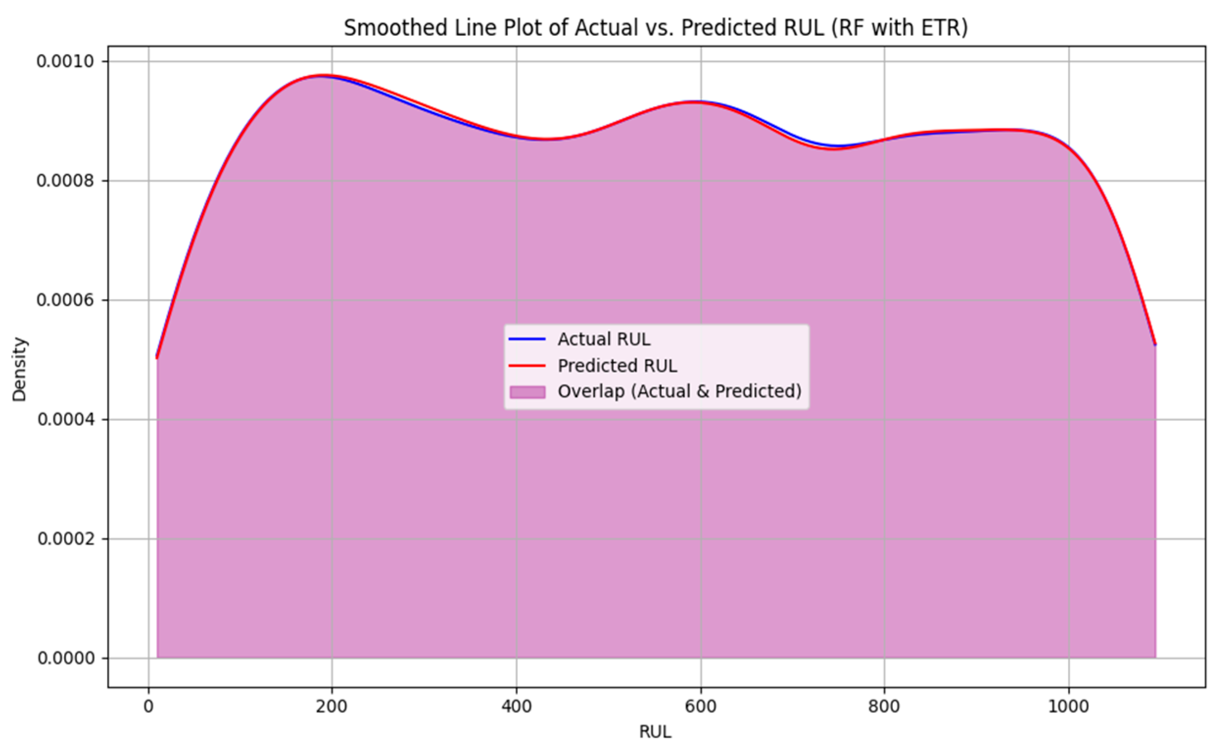
3.3.2. Random Forest with Extra Trees Regressor

Random Forest Regression is a powerful machine learning technique that combines multiple decision trees, each trained on a random subset of data, to make predictions. By aggregating the outputs of multiple trees, the algorithm enhances stability and reduces variance, making it more robust against overfitting. One of its key strengths is its ability to handle complex datasets effectively. Additionally, it introduces an extra layer of randomness by selecting split thresholds randomly rather than strictly optimizing them, allowing for greater generalization in predictive tasks. This added randomness makes the model faster to train, reduces variance, and enhances robustness to noise compared to traditional Random Forest models. Mathematically, the model aggregates predictions from multiple decision trees to generate the final output for the regression problem. For a given set of features where we have $\mathrm{X}=[{\mathrm{x}}_{1, }{\mathrm{x}}_{2,}\dots {\mathrm{x}}_{\mathrm{n},}$] each tree Ti(X) in the ensemble predicts a target value yi, and the final prediction is the average of all tree outputs:

$$\hat{\mathrm{y}}={\displaystyle \frac{1}{\mathrm{N}}}{\sum }_{\mathrm{i}=1}^{\mathrm{N}}\mathrm{T}\mathrm{i}\left(\mathrm{X}\right)$$

where N is the total number of trees in the ensemble, and $\mathrm{T}\mathrm{i}\left(\mathrm{X}\right)$ represents the prediction from the i-th tree. In this study, the Random Forest with Extra Trees Regressor utilizes the entire features to predict the RUL. The n_estimators used = 100, and random_state = 42. All the features, but excluding the cycle count, were utilized to see how it will perform and after which we included all features including the cycle count and compared both performance metrics. For Remaining Useful Life (RUL) prediction, Mean Squared Error (MSE) is a widely adopted loss function in regression-based models such as the Extra Trees Regressor and Random Forest Regressor. As shown in Figure 9, excluding the cycle count as a feature led to a notable gap between the actual and predicted RUL values, with only moderate overlap indicating fair but suboptimal predictive performance. However, when cycle count was included (Figure 10), a visible improvement in overlap between predicted and actual values was observed, reflecting more accurate predictions. To further enhance the model’s performance, we applied hyperparameter tuning to the Random Forest with Extra Trees Regressor. Specifically, we set the number of estimators to 300, the maximum depth to 20, and adjusted the minimum samples required for splits and leaves to 4 and 2, respectively. As illustrated in Figure 10, this significantly increased the overlap between actual and predicted values, minimizing prediction error while also helping to prevent overfitting. Overall, this process led to a more robust and reliable model for RUL estimation.

Figure 9. Distribution of actual vs. predicted RUL using Random Forest with Extra Trees Regressor, without Cycle Count.

Figure 10. Distribution of actual vs. predicted RUL using Random Forest with Extra Trees Regressor, with Cycle Count.

3.3.3. Artificial Neural Network

Artificial Neural Networks are advanced models driven by the function and structure of biological neural networks, such as those in the human brain. These models are widely known for their use in areas requiring high computational power. Some of their uses include pattern recognition, image classification, object detection, and even regression. The architecture of an ANN consists of interconnected nodes, also known as neurons, arranged into three types of layers: the input layer, one or more hidden layers, and the output layer. Each neuron in a layer receives input from the previous layer and processes it with a mathematical function (activation function), which is then passed as output to the next layer. The ANN studies, learns, and understands complex relationships between input and output data through this process. Mathematically, for a single neuron, the output is computed as:

$$\mathrm{z}={\sum }_{i=1}^{N}wixi+b$$

y = σ(z)

• $xi$ represents the input features.
• $wi$ represents the weights assigned to each input.
• $b$ is the bias term.
• σ(z) is the activation function (ReLU or sigmoid) which introduces non-linearity into the model.

Ren et al. [53] proposed an Adaptive Deep Neural Network (ADNN) approach for predicting the remaining useful life (RUL) of lithium-ion batteries. Their method was evaluated using the NASA battery cycle life dataset, where it demonstrated strong performance in multi-battery RUL estimation. The model achieved an RMSE of 6.66% and a prediction accuracy of 93.34%, highlighting its effectiveness in capturing battery degradation trends across different cells. In this study, the ANN model was used to forecast the RUL of lithium-ion batteries by learning patterns in all the features but excluding the cycle counts to see how it will perform and after which we included all features including the cycle count and compared both performance metrics. The ANN architecture consisted of three hidden layers with 128, 64, and 32 neurons respectively, and employed ReLU activation for these hidden layers. Figure 11 shows how the ANN performed with cycle count. As seen below, we observe a high validation loss error with low training loss error and signs of oscillations which indicate overfitting. Now we carried out hyperparameter turning to see if we can remove the oscillations hereby improving the model, this is confirmed by a smooth convergence and strong generalization with no signs of overfitting.

Figure 11. Training and validation loss over epochs for the ANN model.

Regularization techniques such as dropout and L2 regularization were used to prevent overfitting, ensuring the model generalized well to unseen data as evident in Figure 12, the ANN demonstrated the ability to learn non-linear patterns in the data effectively, making it a reliable model for predicting battery health.

Figure 12. Training and validation loss over epochs for the ANN model after hyperparameter tuning.

3.3.4. Long Short-Term Memory (LSTM)

The Long Short-Term Memory (LSTM) is a type of recurrent neural network (RNN) that is well-known for making and processing predictions from sequential data. Its architecture is also used for time series algorithm analysis and natural language sequencing. The design of the LSTM algorithm is crucial for addressing the problem of capturing long-term dependencies in sequential data, which typical RNNs have a limited ability to do. While Transformer-based models and hybrid physics-informed approaches have shown strong potential in recent RUL prediction studies, our focus remains on maintaining a balance between performance and practicality. LSTMs provide reliable results with lower computational demands, making them more suitable for real-world, resource-constrained settings. Given the scale of our dataset and the application context, we opted for a simpler, proven architecture. That said, we acknowledge the value of newer methods and plan to explore them in future work. The choice of an LSTM architecture in this work is motivated by its established strength in modeling temporal dependencies and sequential patterns in battery degradation data. This is particularly important in RUL prediction, where the state of a battery evolves over time through charge-discharge cycles. Zhang et al. [54] demonstrated the effectiveness of LSTM networks for lithium-ion battery RUL estimation in their study on the NASA dataset. These findings support the adoption of LSTM in this work as a reliable architecture for capturing the nonlinear and time-dependent dynamics of battery degradation. Now how the LSTM works is very interesting, we utilized all the features but excluding the cycle counts to see how it will perform and after which we included all features including the cycle count and compared both performance metrics, first an initial decision-making process calculates if the information received from the previous timestamp will be kept or seen as irrelevant and removed. In the subsequent part, the cell makes sure it gets new insights from the received input. Lastly, during the third phase, the cell transfers the updated information from the current timestamp to the subsequent timestamp. Note that a single LSTM cycle is called a one-time step, while the three parts that make up an LSTM unit are called gates. These gates in turn regulate how information is moved into and out of the memory cell in an efficient and effective manner. The initial gate is called the forget gate, the subsequent gate is known as the input gate, whereas the final gate is the output gate. For a provided input sequence $x_t$ at time step t, the LSTM updates its cell state $C_t$ and hidden state $h_t$ as follows:

1.

Forget Gate: Determines which information to discard from the cell state.

$${\mathrm{f}}_{\mathrm{t}}=\mathsf{\sigma }({\mathrm{W}}_{\mathrm{f}}\times \left[{\mathrm{h}}_{\mathrm{t}-1},{\mathrm{x}}_{\mathrm{t}}\right]+{\mathrm{b}}_{\mathrm{f}})$$

2.

Input Gate: Decides which new information to store in the cell state.

$$i_t=\sigma (W_i\times \left[h_{t-1},x_t\right]+b_i)$$

$$\widetilde{C_t}=tanh(W_C\times \left[h_{t-1},x_t\right]+b_C)$$

3.

Cell state update: Combine the forget and input operations to update the cell state.

$$C_t=F_t\times C_{t-1}+i_t\times \widetilde{C_t}$$

4.

Output Gate: Determines the output of the LSTM cell.

$$o_t=\sigma (W_o\times \left[h_{t-1},x_t\right]+b_C)$$

$$h_t=o_t\times \tanh \left(C_t\right)$$

Here, sigma represents the sigmoid activation function, and tanh signifies the hyperbolic tangent function. weights (W) and biases (b) are learned during training.

In this study, LSTM networks are employed to predict the Remaining Useful Life (RUL) of lithium-ion batteries by learning from sequential patterns in the features. Unlike traditional models, LSTMs can effectively model the temporal dependencies in the data, making them highly suited for this task. Training LSTM models involves multiple epochs, where an epoch represents one complete pass through the entire training dataset. During each epoch, the model updates its weights based on prediction error, gradually improving its ability to forecast Remaining Useful Life (RUL). In this study, the model was trained across several epochs to refine its internal parameters and capture the temporal patterns within the battery degradation data. As illustrated in Figure 13, the training and validation loss curves exhibit stable convergence with minimal divergence, indicating strong generalization and a well-balanced learning process. To enhance robustness and mitigate overfitting, Dropout regularization was applied after each LSTM layer, with a dropout rate of 0.3. Additionally, L2 regularization (λ = 0.01) was applied to each LSTM layer to penalize overly complex weights and encourage generalizable patterns. The network ends with a Dense output layer containing a single unit responsible for generating the final RUL prediction. The model was optimized using the Adam optimizer with a learning rate of 0.0001, employing Mean Squared Error (MSE) as the loss function and Mean Absolute Error (MAE) as the performance metric. The final model consisted of 131,489 trainable parameters, resulting in a smooth, consistent learning trajectory and a close alignment between training and validation losses—further validating the effectiveness of the model design and hyperparameter configuration, as shown in Figure 14.

Figure 13. Training and validation loss curves for the LSTM model.

Figure 14. Training and validation loss curves for the LSTM model after hyperparameter tuning.

4. Results and Discussion

The performance of various machine learning algorithms for predicting the Remaining Useful Life (RUL) was evaluated using key metrics as shown in Table 1 and discussed subsequently.

Table 1. Performance Metrics of models without cycle count as a feature.

ML Model	MSE	RMSE	MAE	R2	Training Time (s)	Prediction Time (s)
LSTM	12,291.69	110.87	65.39	0.89	954.72	5.62
LR	3363.206	57.995	44.55	0.90	5.97	0.16
ANN	2456.65	49.56	37.21	0.94	593.54	3.03
RF with ETR	384.27	19.85	8.86	0.98	15.87	0.51

Excluding Cycle Count as a feature resulted in a noticeable drop in overall model accuracy as shown in Table 1. Among the tested algorithms, the Random Forest with Extra Trees Regressor maintained the best performance (R² = 0.98, MAE = 8.86) while offering low computational cost with a training time of 15.87 s and a prediction time of 0.51 s. In contrast, the LSTM model took a much longer training time of 954.72 s, although capable of modeling temporal patterns, showed an R² of 0.89, making it less optimal for fast deployment in edge or low-resource environments.

4.1. Analyzing the Role of Cycle Count and Key Features in Reducing MSE for Lithium-Ion Battery RUL Prediction

We see that as the cycle count of the lithium-ion battery increases, its RUL diminishes. As observed in Table 1, it is vital to notice the high MSE and MAE when compared to Table 2, which shows a relatively high gap between the actual and predicted values. This issue has been addressed and confirms that the cycle count plays a key role alongside other features in forecasting the RUL of lithium-ion batteries.

Table 2. Performance Metrics of models with cycle count as a feature.

ML Model	MSE	RMSE	MAE	R2	Training Time (s)	Prediction Time (s)
ANN	1858.31	43.11	36.06	0.96	276.80	1.61
LSTM	824.15	28.71	12.04	0.97	532.63	2.37
LR	51.86	7.20	4.54	0.98	2.35	0.01
RF with ETR	10.23	3.66	1.99	0.99	7.34	0.05

Including Cycle Count as a feature led to a significant improvement in overall model performance as shown in Table 2. Among all tested algorithms, the Random Forest with Extra Trees Regressor achieved the best results, with an R² score of 0.99, MAE of 1.99, and low computational cost, requiring just 7.34 s to train and 0.05 s to predict. While Linear Regression also performed well (R² = 0.98, MAE = 4.54), it could not capture nonlinear relationships in the data. The LSTM model, although effective in modeling sequential patterns, required substantially more training time (532.72 s) and still yielded an R² of 0.97 which is better than that of the ANN and MAE of 12.04. Similarly, the ANN model performed reasonably well (R² = 0.96), but with a higher MAE of 36.06 and less training time (276.80 s) than it takes the LSTM. Overall, Random Forest with Extra Trees provided the best accuracy, efficiency, and practical balance. As seen, the Extra Tree Regressor model outperforms other models as observed from the values of the MSE and coefficient of determination, which also shows the model’s accuracy. The ability of the extra trees regressor to use multiple parameters for prediction makes it a very powerful model.

It is important to emphasize that the original HNEI database was generated under controlled room temperature conditions, which means the proposed models were trained and tested on datasets under controlled temperature conditions (25 °C) for consistency, but temperature wasn’t included as an input feature. This implies that the model’s predictive accuracy is optimized for standard environments. However, external temperatures such as excessive heat or extreme cold can significantly accelerate battery degradation and negatively impact RUL. Therefore, maintaining batteries at or near 25 °C is ideal to ensure consistent performance and to reduce the risk of spontaneous capacity fading, which could compromise both safety and reliability.

The algorithms were compared based on four main aspects: accuracy, interpretability, time, and computational efficiency, highlighting cross-validation.

4.1.1. Accuracy

Random Forest with extra tree regressor demonstrated the highest accuracy with the lowest MSE (10.23), RMSE (3.66), and MAE (1.99), along with the highest R-squared value (0.99). This performance indicates its exceptional ability to predict RUL with precision. In contrast, Long Short-Term Memory (LSTM) significantly underperformed with high error metrics (MSE: 1858.31) and R-squared value (0.96).

4.1.2. Interpretability

Linear Regression and Random Forest models are highly interpretable due to their straightforward structure, making it easy to trace decision paths and understand feature importance. In contrast, models like Artificial Neural Networks (ANNs) and LSTM operate as “black boxes”, offering limited interpretability despite their moderate predictive capabilities.

4.1.3. Time and Computational Efficiency

Random Forest with Extra Tree Regressor and Linear Regression models are computationally efficient and relatively faster to train than ANN and LSTM, which require extensive computational resources due to iterative processes. LSTM, being a deep learning model, is the most computationally demanding, requiring significant resources for training and inference. The Random Forest with Extra Trees Regressor achieved the fastest runtime, with a training time of 7.34 s and a prediction time of 0.05 s. Other models, such as the ANN and LSTM, required longer training, consistent with the increased computational demands of neural networks and time-series architectures.

4.1.4. Cross Validation

A 5-fold cross-validation was conducted to assess the generalizability and stability of all models. The Random Forest with Extra Trees model achieved the strongest average performance (R² = 0.98, MAE = 2.43, MSE = 12.87), followed by Linear Regression (R² = 1.00, MAE = 4.44, MSE = 49.68). The ANN model performed well with an average R² of 0.95, MAE = 35.24, and MSE = 1842.16, while the LSTM showed good temporal learning capability with an average R² = 0.96, MAE = 11.65, and MSE = 860.92. These results confirm the consistency and reliability of the models across different data splits. A comparison table (Table 3) summarizes our work in relation to previous related studies.

Table 3. Comparison table with existing related works.

References	ML Model	MSE	RMSE	MAE	R2	Training Time	Prediction Time
[9]	Support Vector Machine (SVM)	_	115	_	0.90	_	_
[10]	Random Forest Optimization with HHO	2148.865	46.35	36.88	0.97	_	_
[53]	Adaptive Deep Neural Network (ADNN)	_	6.66	_	0.93	_	_
[11]	Random Forest	14.11	3.75	2.09	0.99	_	0.06
Proposed	Random Forest with Extra Trees Regressor	10.23	3.66	1.99	0.99	7.34	0.05

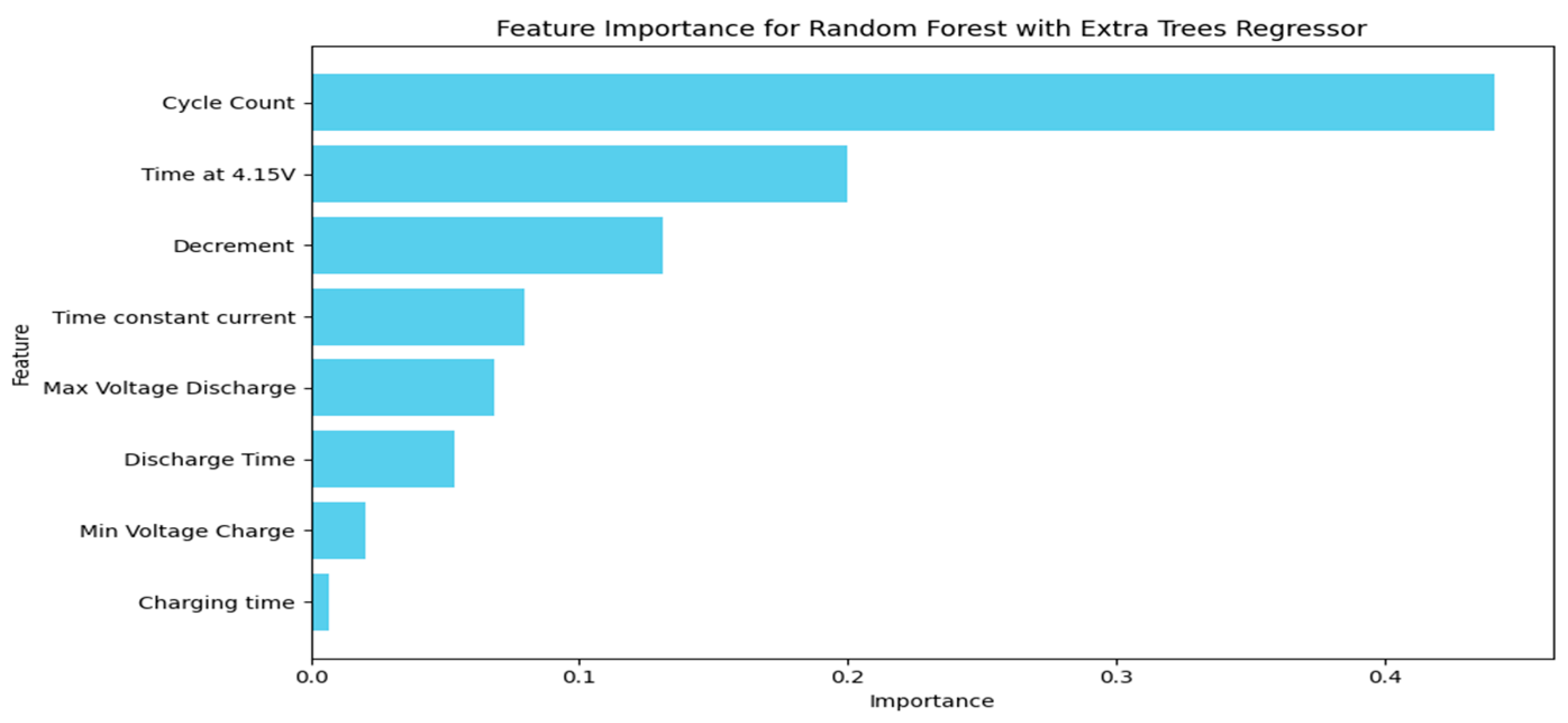
4.2. Feature Importance

Understanding feature importance isn’t just about model performance, it also helps us connect the model’s decisions to what’s happening inside the battery. In our Extra Trees Regressor, Cycle Count is a key predictor when included as seen in Figure 15. The same pattern holds across the other models, too. Now, in the absence of Cycle Count the most important feature was time at 4.15 V as seen in Figure 16, which makes sense since operating near high voltages is known to accelerate SEI (Solid Electrolyte Interphase) layer growth and can lead to lithium plating on the anode surface. Both are key contributors to battery aging. Another top feature, the voltage drop between 3.6 V and 3.4 V, reflects how quickly a battery loses voltage during discharge, which tends to happen faster as the battery degrades. Features like time under constant current and maximum discharge voltage are closely tied to how well the battery holds and delivers energy, which naturally decline with use. Linear Regression places significant emphasis on maximum discharge voltage and minimum charge voltage, optimizing predictions based on their linear relationship with the RUL as seen in Figure 17. Overall, the model’s top features align well with known chemical degradation processes, which helps support the reliability of its predictions.

Figure 15. Feature importance scores for the Extra Trees Regressor with cycle count.

Figure 16. Feature importance scores for the Extra Trees Regressor model without Cycle Count.

Figure 17. Feature importance for the Linear Regression model.

The feature importance for the Artificial Neural Network (ANN) model was determined using permutation-based analysis. The results highlight that Discharge Time is the most significant predictor as seen in Figure 18, contributing the most to the model’s accuracy, followed by Max Voltage Discharge and Time at 4.15 V. Features such as Decrement (3.6 V–3.4 V) and Time Constant Current also show moderate importance, while Min Voltage Charge and Charging Time have comparatively lower impacts. While Random Forest and Extra Trees provide built-in ways to understand which features are most important, LSTM models don’t offer the same level of interpretability out of the box. Although there are advanced methods like permutation importance or SHAP values that can be used, they tend to be more complex and computationally heavy, especially for time-series models like LSTM. To keep the analysis focused and practical, feature importance was only explored for the models where it could be done more directly and clearly. This algorithm analysis underscores the critical role of discharge-related features in predicting the RUL of Li-ion batteries, providing valuable insights for model optimization.

Figure 18. Permutation-based feature importance for the ANN model.

4.3. Web Application Development

A prototype web-based application is designed and developed to provide real-time RUL predictions. The application is built using the following tools:

• Framework: The web application is developed using Streamlit, a Python-based framework known for its simplicity and interactive capabilities. Streamlit allows for rapid prototyping and the creation of visually appealing dashboards and applications. It provides built-in support for integrating machine learning models and simplifies the process of creating forms, charts, and dynamic outputs.
• Backend: The backend of the application is powered by Python, implementing trained machine learning models. These models are algorithms like LSTM, ANN, Random Forest etc., which have been pre-trained on a dataset of lithium-ion battery degradation patterns. Google Colab is utilized for model training and validation due to its cloud-based GPU acceleration, which speeds up computation-intensive tasks. The trained models are exported and integrated into the application for real-time prediction functionality.
• Frontend: The front end is designed with a user-friendly interface to ensure intuitive user experience. Users can input key battery parameters such as charge cycles, temperature ranges, and voltage levels through the application as shown in Figure 19 below. The frontend then displays the predicted RUL alongside visualizations like charts and graphs to provide insights into battery health and degradation trends. Streamlit’s interactive widgets and charts facilitate this process, enhancing usability.
  

  Figure 19. User interface of the web-based simulator app for forecasting the remaining useful life (RUL) of lithium-ion 18650 batteries using machine learning models.
• Deployment: The machine learning models are available on Github Repository, furthermore, to ensure accessibility and scalability, the application is hosted on a cloud platform. Google Colab is used in conjunction with Streamlit and Django for model deployment. By linking our Algorithm on Google Colab notebooks directly to the Streamlit application, real-time predictions can be achieved without requiring extensive local computational resources. The cloud-hosted nature of the application ensures that users can access it from any device with internet connectivity, enabling widespread adoption and utility.

4.4. Benefits and Features

Integrating pre-trained models with the cloud-hosted Streamlit application ensures instantaneous RUL predictions. Cloud deployment allows the application to handle multiple users simultaneously, adapting to varying loads. With minimal computational requirements at the user’s end, the application is accessible to a broader audience. Users can explore battery health metrics through intuitive graphs, enhancing decision-making processes. The modular nature of the application allows for the easy incorporation of additional features, such as comparison across battery chemistry or integration with IoT sensors for real-time data input.

The web application also incorporates Smart Battery Health Classifications, Usage guidelines and Optimization Strategies.

For instance, Excellent Battery Health: RUL between 1112 and 741. Batteries in this range are expected to have a long remaining life and are performing optimally, e.g., Regular Monitoring, Optimal Charging Practices.

Average Battery Health: RUL between 740 and 371. Batteries in this range are functioning, but they are past their peak performance and may require monitoring or eventual replacement, e.g., Conditioning Cycles, Reduced Load.

Low or Poor Battery Health: RUL between 370 and 0. Batteries in this range are nearing the end of their useful life and likely need immediate replacement or significant attention, e.g., Load Reduction, Refurbishment.

5. Conclusions and Future Enhancements

In our case study, Random Forest with Extra Trees Regressor Model is the best-performing model across all evaluated criteria and is recommended for integration into the web-based application for RUL prediction. Linear Regression is a suitable alternative for scenarios requiring simpler implementation with high interpretability. Both LSTM and ANN can perform exceptionally well, especially when there’s enough computational power to support their complexity. Future research could incorporate Transformer-based models or hybrid physics-informed frameworks to evaluate their comparative strengths on the same dataset. Although the original HNEI database was generated under regulated room temperature, our models were also trained and tested using data obtained at 25 °C to guarantee consistency. However, temperature was not included as a modeling input variable. Future researchers could find it beneficial to take temperature as a major consideration when developing predictive models since maintaining batteries at roughly 25 °C helps them perform better and reduces the possibility of rapid capacity loss, which can influence dependability and safety. Furthermore, there should be more focus on extending the application’s capabilities to integrate this machine learning models into EV’s for Real time Management. Features like automated alerts for critical battery conditions, multilingual support, and seamless integration with other battery management systems are planned for subsequent iterations. Additionally, efforts will be made to optimize the computational efficiency of the backend to reduce latency further.

References

1. U.S. Department of Energy. Battery Life and Performance Testing Methodology: PEV Battery Test Manual, Revision 3, INL/EXT-13-30323; Idaho National Laboratory: Idaho Falls, ID, USA, 2015.
2. IEC 61960-3; Secondary Lithium Cells and Batteries for Portable Applications—Part 3: Prismatic and Cylindrical Lithium Secondary Cells and Batteries Made from Them. International Electrotechnical Commission (IEC): Geneva, Switzerland, 2017.
3. Li, J.; Gu, Y.; Wang, L.; Wu, X. A Review of State-of-Health Estimation for Lithium-Ion Batteries. J. Power Sources 2018, 391, 54–60. [Google Scholar] [CrossRef]
4. Jardine, A.K.S.; Lin, D.; Banjevic, D. A Review on Machinery Diagnostics and Prognostics Implementing Condition-Based Maintenance. Mech. Syst. Signal Process. 2006, 20, 1483–1510. [Google Scholar] [CrossRef]
5. Ecker, M.; Tran, T.K.D.; Dechent, P.; Käbitz, S.; Warnecke, A.; Sauer, D.U. Parameterization of a Physico-Chemical Model for Lithium-Ion Batteries Based on Electrochemical Impedance Spectroscopy. J. Power Sources 2012, 215, 248–257. [Google Scholar] [CrossRef]
6. Wang, D.; Wang, Y.; Zhang, J.; Li, H.; Chen, M.; Liu, Q.; Zhao, L.; Huang, X.; Yang, F.; Zhou, Y.; et al. Hybrid Models for Lithium-Ion Battery RUL Prediction. Appl. Energy 2020, 259, 114151. [Google Scholar]
7. Yang, N.; Hofmann, H.; Sun, J.; Song, Z. Remaining Useful Life Prediction of Lithium-ion Batteries with Limited Degradation History Using Random Forest. IEEE Trans. Transp. Electrif. 2023, 10, 5049–5060. [Google Scholar] [CrossRef]
8. Li, J.; Wang, Q.; Du, Z.; Chen, M.; Sun, J. Thermal Runaway Mechanism of Lithium Ion Battery for Electric Vehicles: A Review. Energy Storage Mater. 2018, 10, 246–267. [Google Scholar] [CrossRef]
9. Fei, Z.; Yang, F.; Tsui, K.-L.; Li, L.; Zhang, Z. Early Prediction of Battery Lifetime via a Machine Learning-Based Framework. Battery Res. Adv. 2021, 19, 102–115. [Google Scholar] [CrossRef]
10. Jafari, S.; Byun, Y.-C. Optimizing Battery RUL Prediction of Lithium-Ion Batteries Based on Harris Hawk Optimization Approach Using Random Forest and LightGBM. IEEE Access 2023, 11, 114047–114059. [Google Scholar] [CrossRef]
11. Sekhar, J.N.C.; Domathoti, B.; Gonzalez, E.D.R.S. Prediction of Battery Remaining Useful Life Using Machine Learning Algorithms. Sustainability 2023, 15, 15283. [Google Scholar] [CrossRef]
12. Kumarapp, S.; M, M.H. Machine Learning-Based Prediction of Lithium-Ion Battery Life Cycle for Capacity Degradation Modelling. World J. Adv. Res. Rev. 2024, 21, 1299–1309. [Google Scholar] [CrossRef]
13. Hu, X.; Jiang, J.; Cao, D. Battery health prognosis for electric vehicles using data-driven approaches. Renew. Sustain. Energy Rev. 2017, 75, 301–315. [Google Scholar]
14. He, W.; Chen, H. Cost analysis of predictive maintenance in lithium-ion batteries. Energy Storage Mater. 2019, 18, 420–430. [Google Scholar]
15. Kim, T.; Lim, H.; Cho, B.H. Advances in battery safety through RUL prediction: A review. Prog. Energy Combust. Sci. 2021, 85, 100905. [Google Scholar]
16. Zhang, X.; Wang, L.; Li, J. Sustainability-driven battery management systems: Benefits and challenges. J. Clean. Prod. 2022, 331, 129870. [Google Scholar]
17. Smith, J.; Brown, K. Democratizing Predictive Analytics: The Role of Web Applications. J. Anal. Technol. 2020, 12, 45–62. [Google Scholar]
18. White, A. Centralized Data Management for Predictive Analytics; Springer: Berlin/Heidelberg, Germany, 2019. [Google Scholar]
19. Amazon Web Services. Predictive Maintenance with Amazon Monitron. 2022. Available online: https://aws.amazon.com/solutions/guidance/predictive-maintenance-with-amazon-monitron/ (accessed on 18 March 2025).
20. Li, X.; Zhao, Y. Real-Time Monitoring and Predictive Analytics in IoT Systems. IoT Anal. Rev. 2021, 8, 210–227. [Google Scholar]
21. Khan, M.; Singh, R. Smart Grids: Real-Time Optimization through Predictive Tools. IEEE Trans. Energy Syst. 2021, 15, 300–315. [Google Scholar]
22. Johnson, T. Frameworks for Developing Interactive Dashboards. Int. J. Data Vis. 2022, 14, 50–64. [Google Scholar]
23. Patel, R. User-Centered Design in Predictive Analytics Applications. ACM Comput. Surv. 2021, 53, 120–142. [Google Scholar]
24. Williams, D. Enhancing User Experience with Data Visualization. Data Sci. J. 2020, 10, 67–80. [Google Scholar]
25. Martinez, L.; Carter, P. Enterprise Integration with Predictive Systems. Int. J. Syst. Archit. 2022, 19, 90–102. [Google Scholar]
26. Zhou, H.; Lee, C. Machine Learning Algorithms for Predictive Maintenance Applications; Elsevier: Amsterdam, The Netherlands, 2020. [Google Scholar]
27. Baker, F.; Nguyen, T. Improving Decision-Making with Web-Based Analytics. Harv. Bus. Rev. 2021, 99, 48–54. [Google Scholar]
28. Stevens, G. Standardizing Integration Frameworks for Predictive Analytics. Softw. Eng. Q. 2022, 31, 88–104. [Google Scholar]
29. Hosseini, M. Optimizing Energy Storage Systems with Predictive Maintenance. Arshon Technology Blog. 2024. Available online: https://arshon.com/blog/optimizing-energy-storage-systems-with-predictive-maintenance/ (accessed on 18 March 2025).
30. Bandi, M.; Masimukku, A.K.; Vemula, R.; Vallu, S. Predictive Analytics in Healthcare: Enhancing Patient Outcomes through Data-Driven Forecasting and Decision-Making. J. Mach. Learn. Robot. 2024, 8, 1–20. Available online: https://injmr.com/index.php/fewfewf/article/view/144 (accessed on 11 May 2025).
31. Lee, H.L.; Padmanabhan, V.; Whang, S. Information Distortion in a Supply Chain: The Bullwhip Effect. Manag. Sci. 1997, 43, 546–558. [Google Scholar] [CrossRef]
32. GDPR Advisor. GDPR and Cloud Computing: Safeguarding Data in the Digital Cloud. 2022. Available online: https://www.gdpr-advisor.com/gdpr-and-cloud-computing-safeguarding-data-in-the-digital-cloud/ (accessed on 18 March 2025).
33. Park, E. Model Interpretability in Machine Learning for Non-Experts. Artif. Intell. J. 2020, 17, 210–229. [Google Scholar]
34. Zhang, Y.; Richardson, R.R.; Liu, K.; Howey, D.A. Battery Prognostics under Uncertainty: A Comparative Study and New Prediction Horizon Metric. J. Power Sources 2020, 479, 228806. [Google Scholar] [CrossRef]
35. Kim, H.; Lee, S. A Review of RUL Prediction Models for Variable Operational Environments. Int. J. Progn. Health Manag. 2021, 10, 78–92. [Google Scholar]
36. Li, F.; Zhang, Q. Integrating Predictive Analytics with Practical Systems: Barriers and Opportunities. IEEE Trans. Ind. Inform. 2020, 16, 1234–1243. [Google Scholar]
37. Williams, R. Autonomous Fleet Management Enabled by Predictive Maintenance. Fleet Insights 2023, 8, 34–47. [Google Scholar]
38. Luh, M.; Blank, T. Comprehensive Battery Aging Dataset: Capacity and Impedance Fade Measurements of a Lithium-Ion NMC/C-SiO Cell. Sci. Data 2024, 11, 1004. [Google Scholar] [CrossRef] [PubMed]
39. Gupta, A.; Shukla, D. Developing Open-Access Battery Datasets for Predictive Modeling. Renew. Energy Syst. J. 2022, 9, 89–98. [Google Scholar]
40. Thomas, P.; White, E. Simplifying Predictive Analytics Tools for Non-Experts. J. Hum.-Comput. Interact. 2020, 12, 150–162. [Google Scholar]
41. Johnson, K.; Tran, V. Intuitive Dashboards for RUL Prediction: Design and Implementation. Predict. Insights Q. 2023, 7, 44–59. [Google Scholar]
42. Sun, J.; Zhou, W. Improving Interpretability in Deep Learning Models for Predictive Analytics. AI Ethics 2022, 5, 100–120. [Google Scholar]
43. Paneru, B.; Thapa, B.; Mainali, D.P.; Paneru, B.; Shah, K.B. Remaining Useful Life Prediction for Batteries Utilizing an Explainable AI Approach with a Predictive Application for Decision-Making. arXiv 2024, arXiv:2409.17931. Available online: https://arxiv.org/abs/2409.17931 (accessed on 18 March 2025).
44. Martin, D.; Lopez, M. Data Security in IoT-Based Predictive Systems: A Review. Cybersecur. Priv. J. 2023, 11, 134–148. [Google Scholar]
45. Kumar, N. Balancing Accessibility and Security in Predictive Analytics Platforms. Cloud Comput. Insights 2020, 8, 67–79. [Google Scholar]
46. Stevens, C.; Patel, N. RUL Prediction for Emerging Battery Chemistries. Adv. Battery Technol. 2021, 15, 90–103. [Google Scholar]
47. Wang, Y.; Li, X. Next-Generation Batteries: Challenges in Prognostics and RUL Prediction. Energy Storage Futures 2023, 13, 320–335. [Google Scholar]
48. Rodríguez-Pérez, N.; Domingo, J.M.; López, G.L. ICT Scalability and Replicability Analysis for Smart Grids: Methodology and Application. Energies 2024, 17, 574. [Google Scholar] [CrossRef]
49. Taylor, B. Big Data Processing in Cloud Computing Environments; Wiley: Hoboken, NJ, USA, 2019. [Google Scholar]
50. Doe, J.; Smith, A. Advancements in AI for Energy Management. Energy Technol. J. 2023, 15, 100–115. [Google Scholar]
51. Lacy, F.; Ruiz-Reyes, A.; Brescia, A. Machine learning for low signal-to-noise ratio detection. Pattern Recognit. Lett. 2024, 179, 115–122. [Google Scholar] [CrossRef]
52. Ding, T.; Xiang, D.; Sun, T.; Qi, Y.; Zhao, Z. AI-Driven Prognostics for State of Health Prediction in Li-ion Batteries: A Comprehensive Analysis with Validation. arXiv 2025, arXiv:2504.05728. [Google Scholar]
53. Ren, L.; Zhao, L.; Hong, S.; Zhao, S.; Wang, H.; Zhang, L. Remaining useful life prediction for lithium-ion battery: A deep learning approach. IEEE Access 2018, 6, 50587–50598. [Google Scholar] [CrossRef]
54. Zhang, Y.; Xiong, R.; He, H.; Pecht, M.G. Long short-term memory recurrent neural network for remaining useful life prediction of lithium-ion batteries. IEEE Trans. Veh. Technol. 2018, 67, 5695–5705. [Google Scholar] [CrossRef]
Disclaimer/Publisher’s Note: The statements, opinions and data contained in all publications are solely those of the individual author(s) and contributor(s) and not of MDPI and/or the editor(s). MDPI and/or the editor(s) disclaim responsibility for any injury to people or property resulting from any ideas, methods, instructions or products referred to in the content.
Article Metrics
Citations
Article Access Statistics
Multiple requests from the same IP address are counted as one view.