An Automated Framework for Streamlined CFD-Based Design and Optimization of Fixed-Wing UAV Wings

Abstract

The increasing complexity of the UAV aerodynamic design, imposed by novel configurations and requirements, has highlighted the need for efficient tools for high-fidelity simulation, especially for optimization purposes. The current work presents an automated CFD framework, tailored for fixed-wing UAVs, designed to streamline the geometry generation of wings, mesh creation, and simulation execution into a Python-based pipeline. The framework employs a parameterized meshing module capable of handling a broad range of wing geometries within an extensive design space, thereby reducing manual effort and achieving pre-processing times in the order of five minutes. Incorporating GPU-enabled solvers and high-performance computing environments allows for rapid and scalable aerodynamic evaluations. An automated methodology for assessing the CFD results is presented, addressing the discretization and iterative errors, as well as grid resolution, especially near wall surfaces. Comparisons with the results produced by a specialized mechanical engineer with over five years of experience in aircraft-related CFD indicate high accuracy, with deviations below 3% for key aerodynamic metrics. A large-scale deployment further demonstrates consistency across diverse wing samples. A Bayesian Optimization case study then illustrates the framework’s utility, identifying a wing design with an 8% improvement in the lift-to-drag ratio, while maintaining an average $y^{+}$ value below 1 along the surface. Overall, the proposed approach streamlines fixed-wing UAV design processes and supports advanced aerodynamic optimization and data generation.

1. Introduction

In recent decades, fixed-wing UAVs have found an increasingly diverse range of applications, including precision agriculture [1], cargo transport [2], and environmental monitoring [3]. UAVs can also be used for beach monitoring [4] and search and rescue situations in various environments [5] (i.e., forests and mountains, as well as highly densely populated areas). This growth is guided by advancements in autonomy, propulsion systems, and materials, enabling UAVs to meet evolving operational demands while maintaining adaptability for a broad spectrum of missions.

Despite these advancements, the design methodologies for fixed-wing UAVs largely resemble the “traditional” design methods employed for manned aircrafts [6,7]. The latter have evolved through a systematic, iterative, human intensive approach segmented into three primary stages: conceptual, preliminary, and detailed design. The conceptual phase lays the groundwork by defining high-level system requirements and exploring multiple configurations to address mission-specific criteria. At this phase, which is marked by significant uncertainty, rapid prototyping and multiple testing of various configurations are key to advances in the next stages. The need for the exploration of the design space before progressing requires the utilization of low-fidelity and semi-empirical methods to assess the impact of alterations, typically in geometry. The preliminary phase refines these configurations through focused analyses of key components, ensuring alignment with performance, stability, and manufacturability goals. Computational Fluid Dynamics (CFD) analyses are fundamental for assessing aerodynamic performance and optimizing UAV designs, especially in this stage. High-fidelity methods, such as Reynolds-Averaged Navier–Stokes (RANS) simulations, require detailed meshes that can be laborious to generate and validate, adding significant overhead to the design process. It is acknowledged that experimental testing, particularly with rapid prototyping (RP), remains fundamental in fixed-wing UAV development. However, conducting wind tunnel tests often requires significant infrastructure, including specialized facilities, calibration procedures, and trained personnel, making it resource-intensive—especially for large-scale UAVs in the tactical, MALE, and HALE categories [8]. In contrast, CFD provides a standardized and reproducible method for systematically analyzing multiple design variations in design offices, acting as a third way of analyzing engineering problems, in addition to theoretical relations and experiments [9]. Consequently, CFD is often the primary tool for aerodynamic assessment, while experimental testing serves as a crucial validation step where resources permit.

Finally, the detail design phase involves the details of the selected configuration, including the construction drawings, resolving all remaining uncertainties to deliver a prototype. This structured, iterative process, while effective, underscores the resource-intensive nature of fixed-wing UAV development.

This is even more evident when addressing specialized applications or unconventional configurations. Especially concerning the latter, and following the design trends of modern aviation, novel configurations are investigated [2,10,11] and new lift and drag estimation methods are introduced to assist in the early stages of development [12]. Among these novel configurations, Blended Wing Body (BWB) designs are gaining significant attention due to their potential to improve aerodynamic efficiency, increase payload capacity, and reduce fuel consumption. Unlike conventional UAV designs, BWBs integrate the fuselage and wings into a unified aerodynamic shape, which presents unique advantages and challenges in aerodynamic analysis. These designs are particularly relevant for missions demanding long endurance and high efficiency, such as surveillance or cargo delivery, making them a prime focus for modern research frameworks [13]. The framework presented in this study addresses these challenges directly by automating the generation and analysis of both conventional and BWB UAV meshes, emphasizing their potential importance in future UAV developments.

Several studies have explored the potential for fully automating the time-intensive phase of aerodynamic evaluation [14,15,16]. These works highlight specific algorithmic strategies to accelerate aspects of the design process, such as focusing on the solution phase alone, automating calculations (e.g., decomposing forces into lift and drag), or employing high-performance computing. Other research efforts have adopted a more holistic approach to address the problem comprehensively.

Specifically, in [17], the authors developed a framework to automatically handle mesh generation and CFD analysis. However, their analysis is limited to simple trapezoidal subsonic UAV wing planforms. Additionally, the study in [18] examined the efficiency of multi-fidelity algorithms that combine low-fidelity panel methods with CFD for Blended Wing Body (BWB) UAVs. Their approach began with a baseline geometry, which was deformed using Free-Form Deformation (FFD). This study, though, offers constrained degrees of freedom within the design space, as the configuration cannot deviate from a given baseline, e.g., providing no degrees of freedom in terms of wingspan. Furthermore, in [19], the authors applied FFD to locally morph computational grids and perform optimization studies using RANS CFD simulations. Similarly, in [20], researchers focused on validating an automated CFD chain, creating a Python-based framework that integrated multiple software tools for geometry manipulation. Both the above works, however, are limited to a specific baseline configuration, e.g., the Common Research Model in [19]. Moreover, studies [21,22] introduced machine learning methodologies for optimizing UAVs, including wings, fuselage, and engine configurations, by using high-level parameters (e.g., aspect ratio, wingspan, taper ratio, or thrust for engines) and targeting specific Unmanned Combat Aerial Vehicle (UCAV) designs. These works employed neural networks trained on low-fidelity panel data generated from frameworks capable of sampling design spaces, creating geometry models, and conducting analyses. Although these studies present a promising foundation that could potentially integrate CFD data, they do not eventually involve CFD results, which limits the fidelity and applicability of their optimization frameworks.

To cover the aforementioned research gaps, this study aims to develop an innovative, robust, and streamlined framework employing high-end commercial software to enable fully automated, high-fidelity CFD analyses of UAV wings. More specifically, the key objectives of this work are as follows:

• Provide a general algorithm for automation of CFD-based investigations. All aspects are based on an extensive literature survey at every part of the study, combining well-established common practices with proposed novel algorithms that unify all the components. Due to budget constraints, the authors could not develop the framework to work with all possible software alternatives. However, in case other research groups want to employ a different software, they will only have to emphasize specific parameters, and the overall architecture will remain as suggested.
• In contrast to existing frameworks that focus on given platforms or narrow design spaces, examine an extensive design space, allowing its application to the vast majority of UAV configurations [8].
• Accommodate wings for both conventional and tailless configurations (flying wings, BWBs), while incorporating a set of 35 design parameters that can completely control the wing planform and its airfoils.
• Apart from presenting the pipeline, suggest robust evaluation criteria and metrics in an automated format.

It must be noted at this point that, based on these objectives, this work aims to present and demonstrate a comprehensive algorithm and its corresponding framework, transitioning from geometry to simulation. The validation against experimental or flight-testing data is beyond the scope of this study, as the individual methods have already been validated in prior non-automated studies.

This paper proceeds as follows: Section 2 provides a detailed overview of the design space, focusing on UAV types and wing geometry parameterization. Section 3 outlines the framework’s components, including its integration of OpenVSP (v3.40.1), BETA CAE ANSA (v24.2.1, Root, Switzerland), and ANSYS Fluent [v2023 R2], with detailed sub-algorithms for each module. Section 4 discusses the evaluation metrics used to quantify errors from mesh generation and introduces a novel rapid assessment method for CFD results. In Section 5, the computational grid is validated against common geometries and expert benchmarks, supplemented by a large-scale deployment to assess result quality. Finally, the adaptability of the framework is demonstrated through an optimization case study, which highlights its capability to automate CFD pre-processing and analysis within constrained design spaces.

2. Design Space

This study organizes the design space into two components: geometric design space and flow conditions design space.

• The geometric design space defines the shape of the wing, including planform parameters and airfoil shapes, which dictate the aerodynamic performance of UAVs.
• The flow conditions design space considers environmental and operational parameters such as velocity and altitude, which influence aerodynamic performance under different mission scenarios.

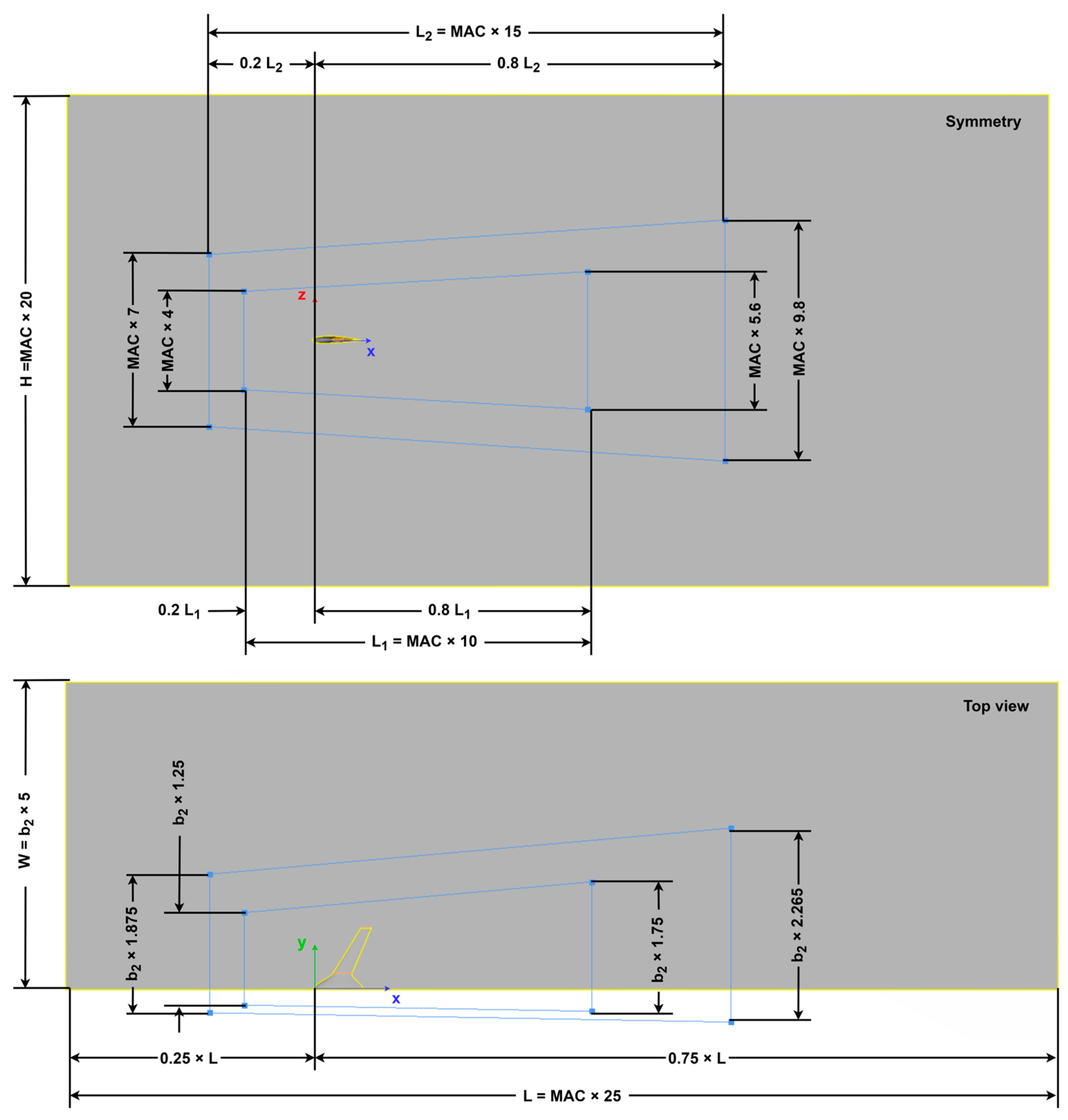
Specifically, the wing geometries and flow conditions incorporated into the framework are derived from a diverse set of UAVs and their respective operational conditions. The design space includes UAVs ranging from the Micro class (<2 kg MTOW) to MALE and HALE-Strike categories (>600 kg MTOW), as classified by NATO and detailed in [8].

Table 1. Design space regarding the UAV types that this framework can handle.

Class	Category	GTOW [kg]	Altitude [ft]	Cruise Speed Range [km/h]	Reynolds Number Range	Flow Regime
Class I	Micro	$<2$	$<200$	$30–100$	${10}^4–{10}^6$	Laminar to Transitional
	Mini	$2–15$	$<3000$	$30–100$
	Small	$15–150$	$<5000$	$50–150$
Class II	Tactical	$150–600$	$<\mathrm{18,000}$	$100–400$	${10}^6–{10}^7$	Predominantly turbulent
Class III	MALE	$>600$	$<\mathrm{45,000}$	$200–300$	$>{10}^7$	Fully turbulent
	HALE	$>600$	$<\mathrm{65,000}$	$400–800$
	Strike	$>600$	$<\mathrm{65,000}$	$400–800$

summarizes these UAV categories along with their associated operating conditions.

The following sections elaborate on the geometric and flow conditions design space, detailing how they are parametrized and integrated into the framework to accommodate this wide range of UAV designs. Although this framework also covers conventional planforms, particular attention is given to tailless and Blended Wing Body (BWB) configurations, which, despite not being universally optimal for all missions, remain an important research focus in modern aviation. This is evidenced by multiple global initiatives—such as NASA’s X-48 and X-56 prototypes [23,24]—and the recent EU-funded EXAELIA project [25], whose flight demonstrators prominently feature BWB architectures. Moreover, BWBs pose complex challenges in simultaneously achieving lift generation and flight stability, making them valuable for testing and refining the framework’s capabilities. Thus, they serve as exemplary case studies even if they are not invariably the most efficient choice for every UAV application.

2.1. Geometric Design Space and Parametrization Techniques

To enable fully autonomous geometry generation without human intervention, the wing planform must be parameterized in such way as to account for the degrees of freedom necessary for a designer during the conceptual and preliminary stages of UAV design. For the wing parametrization, the current study employes “low-level” variables, such as wing chords ($c_r$, $c_t$) and wingspan (b), which offer a clearer and more practical representation of geometry.

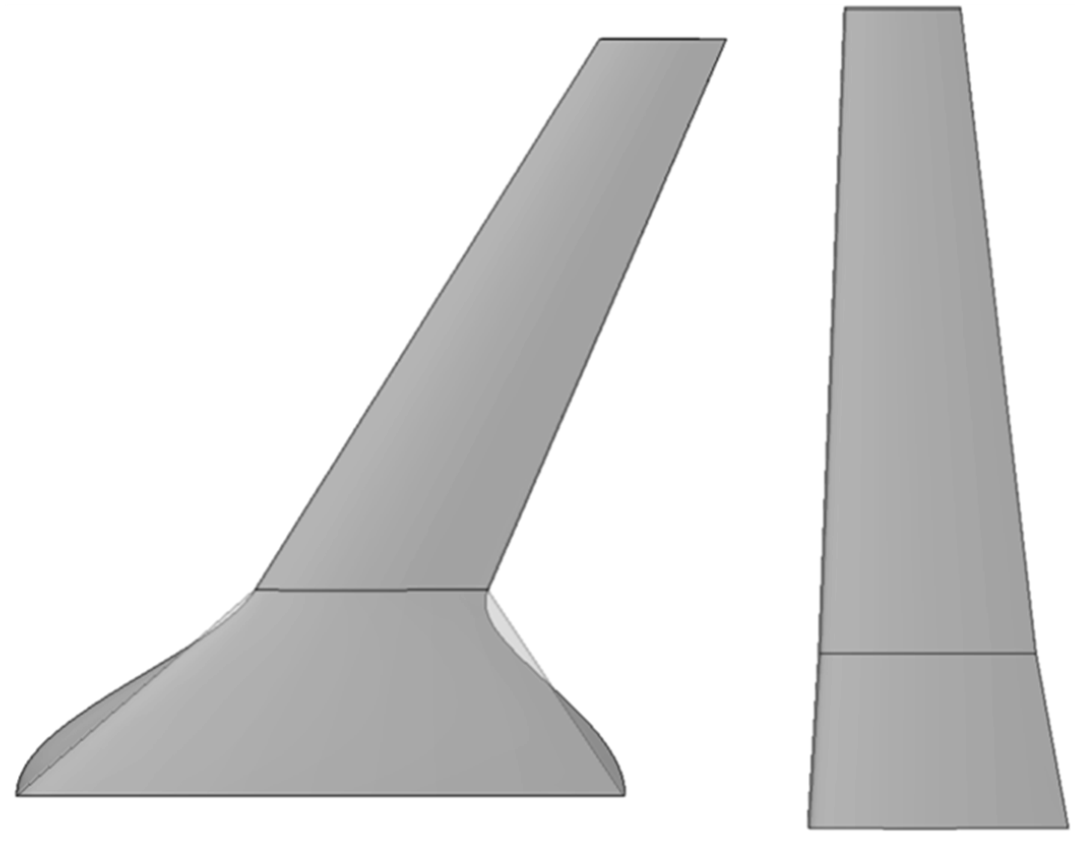
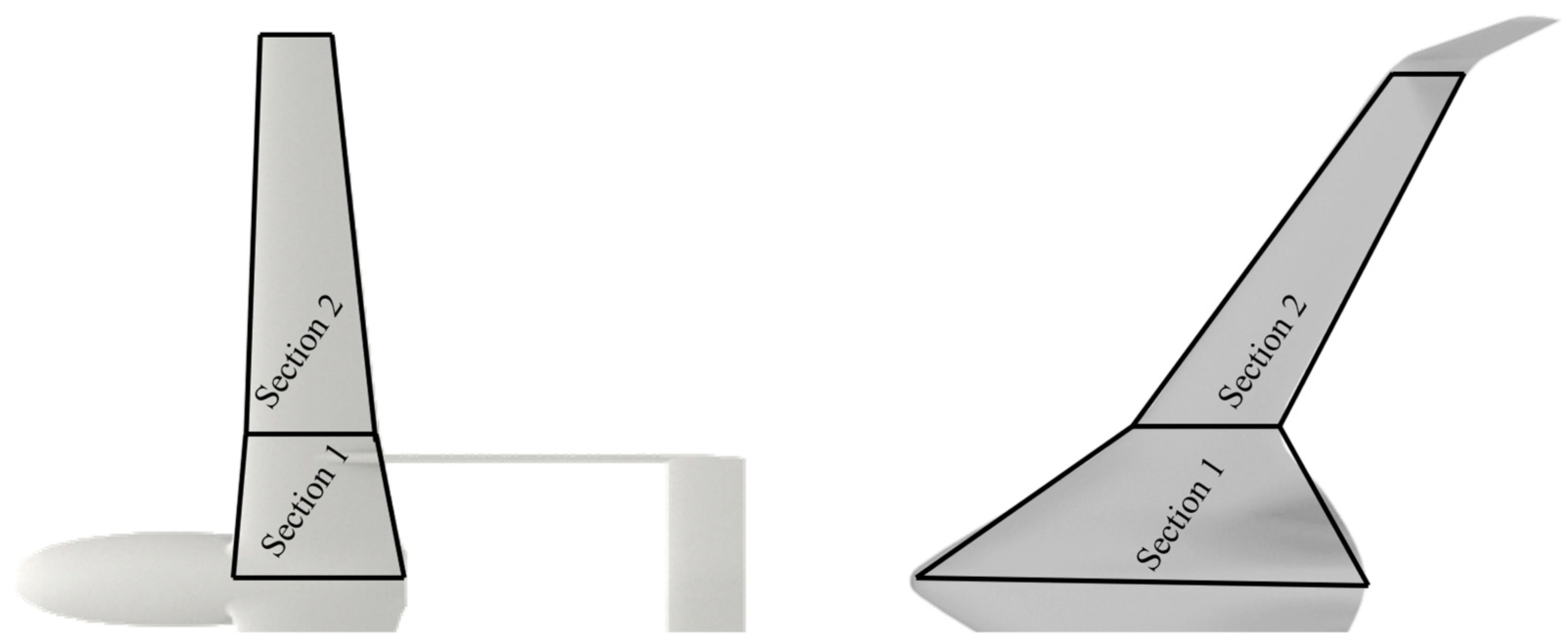
The design space accommodates both conventional and BWB UAVs. Conventional UAV wings are typically defined with one or two sections (i.e., the distinct trapezoidal planform surfaces that constitute the wing, are referred to as wing sections), as seen in Figure 1, and are differentiated from the rest of the aircraft. In contrast, BWB UAVs have a more integrated structure, where the “fuselage-body” and wings blend into a continuous aerodynamic shape, as seen in Figure 1.

In most cases, and especially for BWB configurations, accurately capturing the complexity of the geometry requires multiple sections [26]. However, each additional section increases the number of design variables, leading to higher dimensionality in the design space. While greater dimensionality allows for detailed representations and subtle geometric variations, it also significantly increases computational costs during optimization. This framework restricts the design space for both conventional and BWB UAVs to two distinct trapezoidal sections which are smoothly blended to avoid sharp transitions, as explained in Section 3.1. While this parameterization includes non-planar features (dihedral), it does not currently incorporate additional non-planar elements like winglets, flaps, or slats. This limitation simplifies the geometry and meshing processes at this stage, providing a stable basis that can be extended to more complex design spaces in the future.

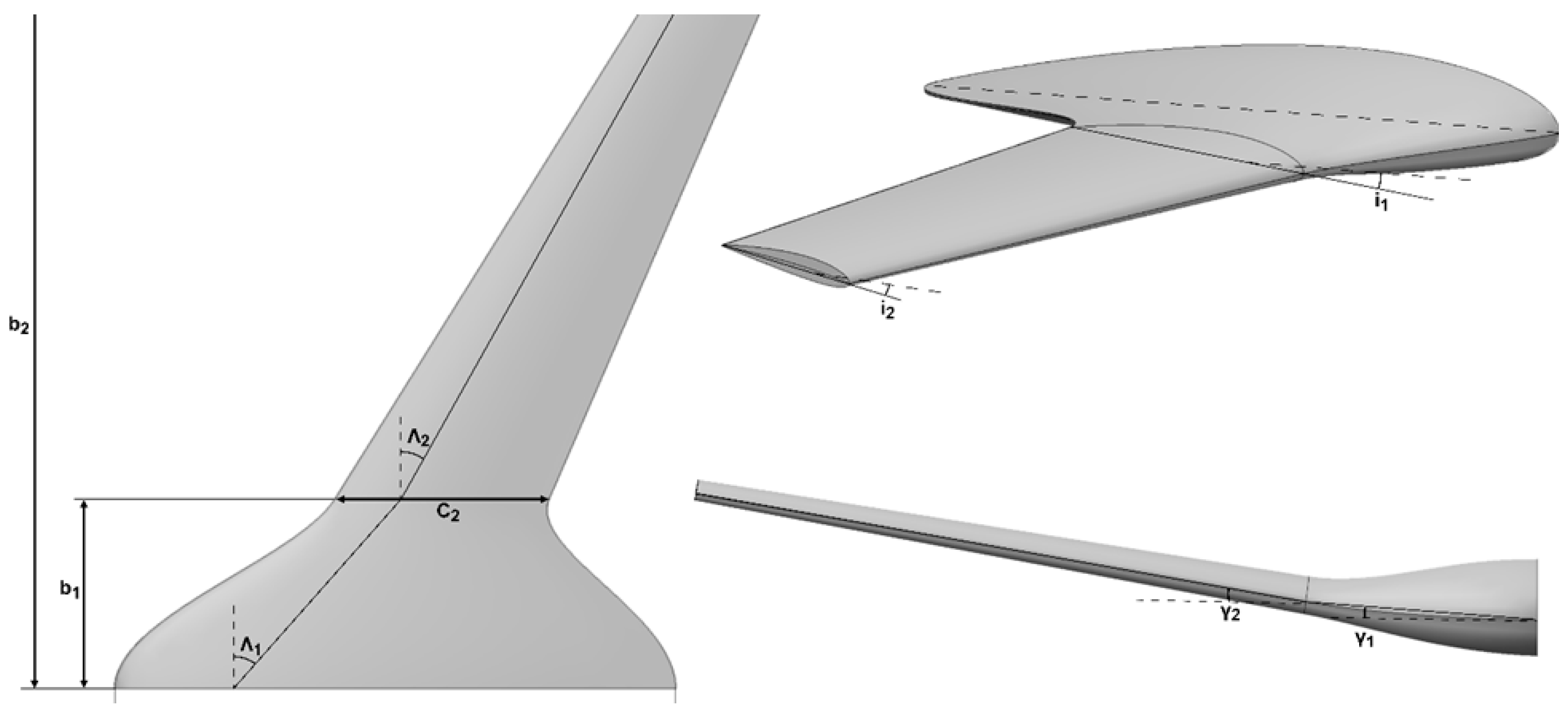
The necessary parameters and their respective range that define the planform of a wing instance for both configurations are tabulated in

Table 2. Design variables used to parameterize the wing planform and their respectable range.

Planform Parameter	Description	Units	Limits
$c_1$	Centerline chord length	$\mathrm{m}$	$c_1\in [0.2, 10]$
$c_2$	Root chord length	$\mathrm{m}$	$c_2\in [0.3\times c_1, c_1]$
$c_3$	Tip chord length	$\mathrm{m}$	$c_3\in [0.3\times c_2, c_2]$
$b_1$	$c_2$ spanwise location	$\mathrm{m}$	$b_1\in [0.2\times b_2, {0.7\times b}_2]$
$b_2$	$c_3$ spanwise location (semispan)	$\mathrm{m}$	$b_2\in [1, 10]$
${\Lambda }_1$	$\mathrm{Sweep} \mathrm{angle} \mathrm{of} \mathrm{section} 1@c/4$	$\mathrm{d}\mathrm{e}\mathrm{g}$	${\Lambda }_1 \in [0, 60]$
${\Lambda }_2$	$\mathrm{Sweep} \mathrm{angle} \mathrm{of} \mathrm{section} 2@c/4$	$\mathrm{d}\mathrm{e}\mathrm{g}$	${\Lambda }_2 \in [0, 60]$
$i_1$	$\mathrm{Twist} \mathrm{angle} \mathrm{of} c_2$$@c/4$	$\mathrm{d}\mathrm{e}\mathrm{g}$	$i_1 \in [-5, 5]$
$i_2$	$\mathrm{Twist} \mathrm{angle} \mathrm{of} c_3$$@c/4$	$\mathrm{d}\mathrm{e}\mathrm{g}$	$i_2 \in [-7, 7]$
${\gamma }_1$ ${\gamma }_2$	Dihedral angle of section 1	$\mathrm{d}\mathrm{e}\mathrm{g}$	${\gamma }_1 \in [-10, 10]$
	Dihedral angle of section 2	$\mathrm{d}\mathrm{e}\mathrm{g}$	${\gamma }_2 \in [-10, 10]$

and are also depicted in Figure 2.

A total of 11 low-level parameters are required to fully define the planform of a two-section wing, without including any details about the airfoil shape. It should be noted that all parameters are referenced from the coordinate system with an origin on the leading edge of the centerline chord. The x-axis spans along the chordwise direction and the y-axis spans along the spanwise direction of the wing.

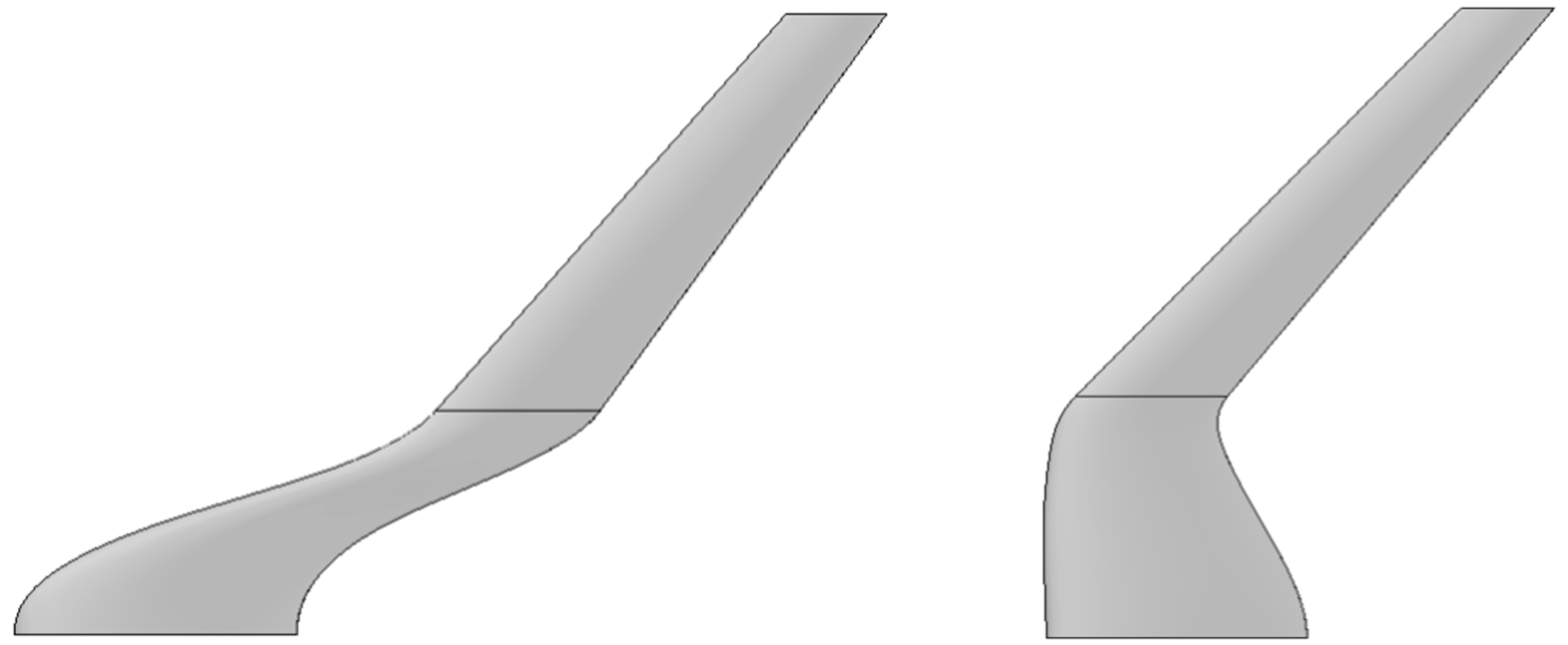
Design variable constraints have been defined to exclude unrealistic wing geometries such as having taper ratio values larger than 1, wings with very thin sections that would be impossible to manufacture, or wings with excessive aft and forward sweep angles (Figure 3). These parameters, combined with constraints, ensure that the design space remains realistic and aligned with established aerodynamic standards.

The wing’s cross-section is defined by three distinct airfoils: one at the root, one at the kink (midsection break), and one at the tip. Airfoil profiles are assigned to these spanwise locations, with interpolation between them. The airfoil shape greatly affects the aerodynamic characteristics of wing geometry. The precise shape of an airfoil can vary greatly depending on its intended use, flight conditions, and performance requirements. One of the most common airfoil databases is the one from UIUC [27], which contains more than 1500 airfoil shapes from real cases. Selecting airfoils based on their unique categorical identifiers transforms the design space into a high-dimensional, discrete domain. This discrete nature lacks the continuity required for efficient aerodynamic shape optimization, where smooth transitions between design variables are essential. To address this, parameterization techniques that represent airfoil shapes through continuous variables are employed.

Common parametrization techniques include the Bézier–PARSEC method, Class Function/Shape Function Transformations (CST), B-Splines combined with dimensionality reduction techniques such as Principal Component Analysis (PCA), and others [28]. However, the main drawbacks of those methods are the generation of non-smooth trailing edges with the frequent crossing of the lower pressure surface and the upper suction one and the demand of a large amount of design to accurately represent the airfoil in terms of geometric similarity and aerodynamic performance. Given these challenges, a novel approach to airfoil parameterization was required—one that could achieve high shape diversity while maintaining a low dimensionality for efficient optimization. The method adopted in this study is based on the Bézier–GAN (BGAN) parameterization technique, developed by Chen, Chiu, and Fuge from the University of Maryland [29]. This deep learning model, based on Info-GAN structures, specifically designed for aerodynamic shape generation, leverages the smooth, continuous properties of Bézier curves within a GAN framework to produce realistic airfoil shapes.

These networks utilize latent codes and noise variables as inputs to the network, to effectively capture both major and minor shape variations in airfoils, enabling the synthesis of smooth, aerodynamic designs. The latent codes form a low-dimensional representation that serves as the primary mechanism for representing major shape features, such as thickness, camber, reflex, and overall curvature. Alongside the latent codes, noise variables can be introduced to handle finer, more detailed aspects of the airfoil shape. These noise variables provide an additional level of granularity, allowing for subtle adjustments that add diversity to the generated shapes. Following the training methodologies proposed by Chen et al., the parameters depicted in

Table 3. Training parameters for the BGAN model.

Training Parameter	Value	Description
Bézier degree	32	The number of Bézier control points
Latent codes dimension	8	Number of latent codes
Noise dimension	0	Number of components in noise vector
Train steps/epochs	150,000	-
Batch size	32	Number of samples per network pass
Bounds	[0, 1]	Bounds of latent codes and noise components
Latent code sampling PDF	Uniform	Probability distribution

are selected to train the airfoil generator.

Thus, with only eight design variables, it is possible to accurately represent an airfoil that belongs in the original UIUC database (training dataset), as well as to generate new novel configurations that enhance the exploration of the design space. It is important to note that while the UIUC database primarily contains airfoils analyzed at low Reynolds numbers, the BGAN training dataset utilizes only the geometry of the airfoils and not the results of the corresponding analyses. Moreover, many of the airfoils in the database are widely used in operating aircrafts, where they perform effectively at significantly higher Reynolds numbers.

2.2. Operating Conditions

The design space for this framework is confined to the subsonic regime, where flow velocities remain below Mach 0.3. This range is representative of typical UAV operational conditions according to [8,30,31] and ensures that compressibility effects can be neglected. Within this regime, velocities primarily influence computational mesh and turbulence modeling strategies. Table 1 highlights that each UAV class operates under different conditions without a uniform trend applying to all classifications. The selected operational design space is dependent on the wing geometry, which is sampled from the geometric design space. The altitude was kept constant (at sea level) for all wings, while the cruise speed was sampled within the range defined individually for each UAV class [8,32].

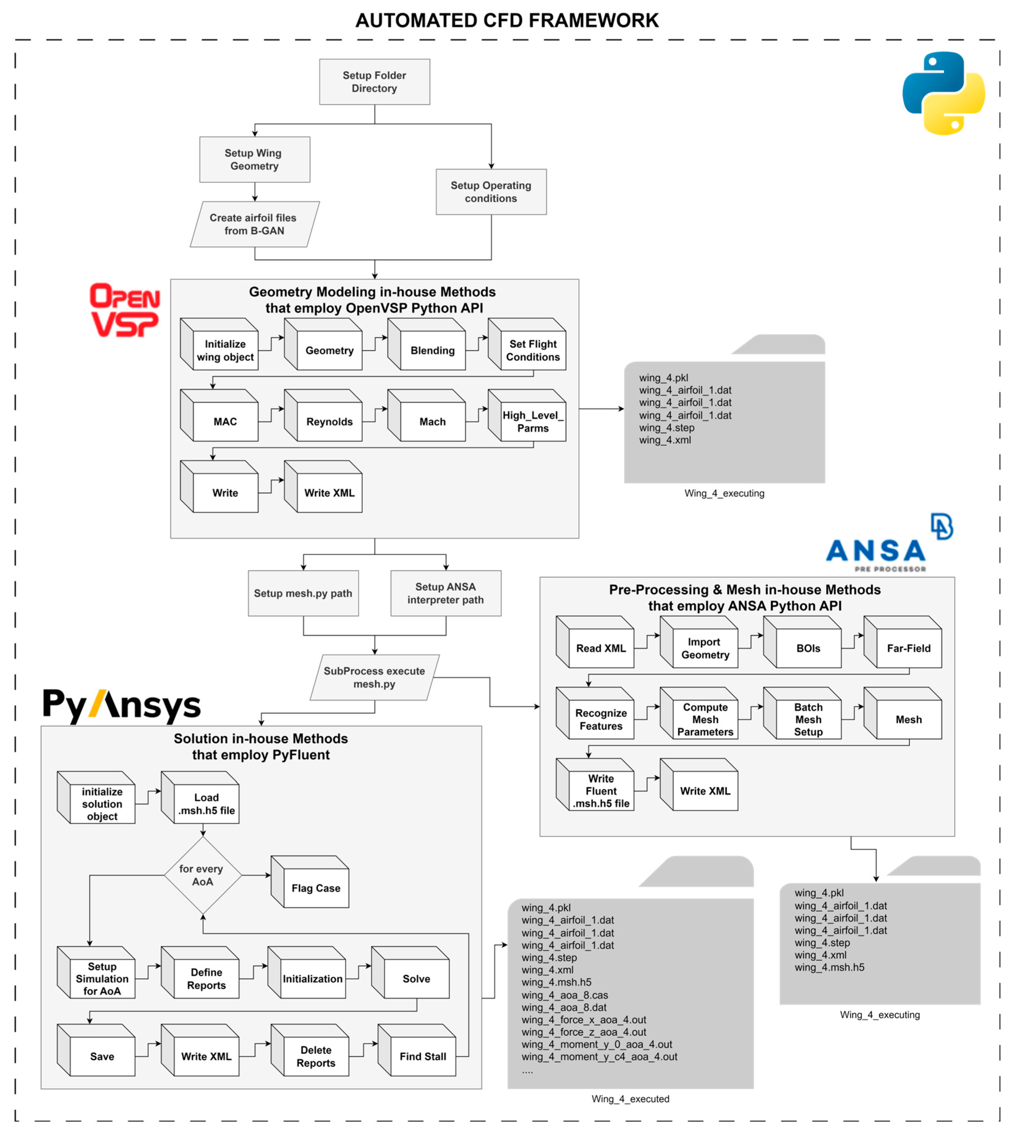
3. Framework Breakdown

The proposed framework automates the CFD workflow for UAV wings, integrating geometry generation, meshing, and simulation execution into a Python-based pipeline, as illustrated in Figure 4. It eliminates manual intervention, promotes consistency across a large design space, and significantly accelerates the aerodynamic evaluation process for both individual case studies and optimization-driven analyses.

The three modules are as follows:

• Geometry Modeling: Utilizes OpenVSP’s Python API [33] for generating 3D UAV wing models. Implemented using an object-oriented programming (OOP) approach, the geometry module employs a Wing class that encapsulates design parameters, flight conditions, and methods for geometry generation and blending.
• Meshing: Utilizes BETA CAE’s ANSA pre-processor [34] to transform geometries into solver-ready grids, adhering to stringent quality standards for subsonic flows.
• Simulation Execution: Employs ANSYS Fluent via the appropriate API—PyFluent (v0.21) [35], a module for automating simulation setup, execution, and result post-processing.

The framework relies on XML files for data exchange between modules, allowing for consistent information flow. As presented in Section 5, high-performance computing (HPC) with the GPU-native Fluent solver significantly enhances computational efficiency, reducing processing times and enabling rapid CFD analysis execution.

An important comment must be made regarding the turbulence modeling approach, since it affects two latter key modules (meshing and solution). Several main approaches are encountered in the CFD literature, balancing accuracy and computational cost. Direct Numerical Simulation (DNS) resolves all turbulence scales but is computationally impractical for most applications, due to its high computational cost. Large Eddy Simulation (LES) resolves larger turbulent structures while modeling smaller eddies, requiring significant resources, especially for optimization purposes when the number of required solutions is in the hundreds or thousands, depending on the optimization study [17]. However, Reynolds-Averaged Navier–Stokes (RANS) models offer computational efficiency suitable for steady-state aerodynamic analyses, making them the industry standard [36,37].

In this study, the RANS approach with Menter’s k-omega SST [38] turbulence modeling is adopted, validated through prior work against both in-house test flight data and assessed against experimental results [39]. While this validation confirms its suitability within the design space intended, it is important to note that the model has not been explicitly validated for every possible wing configuration that may arise from the sampling of this space. However, its extensive use in similar studies further supports its applicability to this framework [40]. This choice is made to align with the computational tools available, specifically the GPU-native solvers in the utilized version of ANSYS Fluent 2023R2 [41,42].

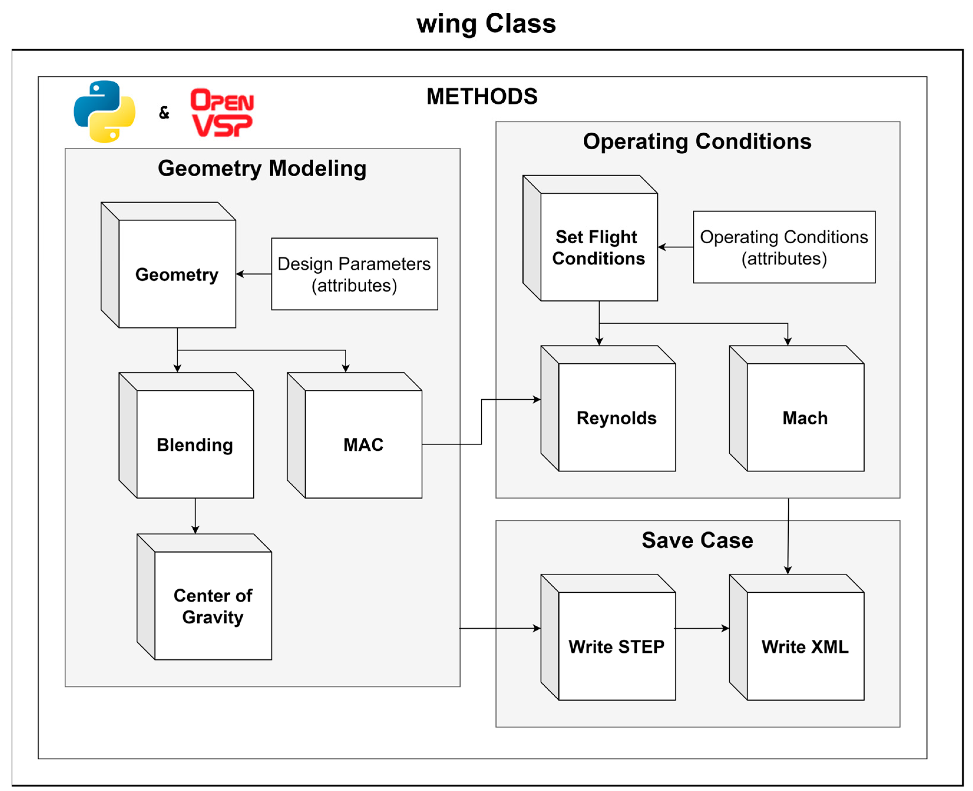
3.1. Geometry Module

The geometry module is critical for generating CFD-ready wing geometries, ensuring compatibility with the following meshing and simulation processes. According to [41], a “good” geometric model tailored to the requirements of CFD not only enhances workflow efficiency but also ensures reliable and reproducible results—an essential objective of this framework, where robustness is paramount. Using an object-oriented programming approach, the module features a dedicated Wing class, as shown in Figure 5.

The Wing class methods can be distinguished into three categories:

• Geometry Modeling: involves defining design parameters and producing the core geometry, automating blending between sections, calculating the Mean Aerodynamic Chord (MAC), and determining the center of gravity.
• Operating Conditions: definition of flight conditions and computation of key metrics.
• Case Management: exports geometry in STEP format and records attributes in an XML file for case tracking.

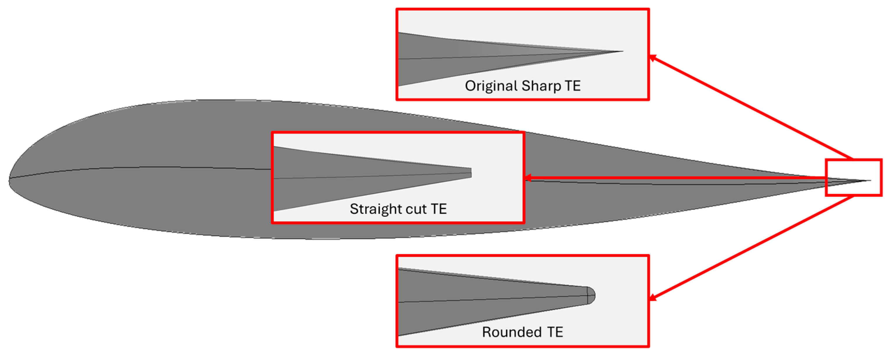
Trailing edge (TE) treatment, section blending, and Mean Aerodynamic Chord (MAC) calculation are integral to ensure that the generated wing geometries are appropriate for CFD meshing. The trailing edge cut is applied to improve mesh quality and numerical stability, as sharp TEs often lead to a high aspect ratio or skewed cells, affecting solver convergence [42]. To maintain consistency, the TE thickness is set to 1% of the chord length, a commonly recommended guideline for subsonic applications [41]. Blending between wing sections is fully automated to eliminate abrupt transitions, ensuring geometric continuity across all generated designs. The framework prioritizes the second section as the primary lifting surface, with the first section adjusted to enforce tangency at the leading and trailing edges, preventing discontinuities at the symmetry plane.

Additionally, the MAC is computed using a weighted averaging approach, serving as the reference chord length for moment coefficient (Cm) calculations, which define the pitching moment characteristics of the wing about its aerodynamic center [7]. Moreover, MAC serves as the characteristic length for the calculation of the Reynolds number. These treatments eliminate human intervention and are executed in the background, minimizing the workload needed for geometry preparation. Further details on TE treatment methodology, blending algorithms, and MAC computation are provided in Appendix A.1.

The right-hand side of Figure 5 highlights additional capabilities of the geometry module. While these functions, such as the calculation of Reynolds and Mach numbers, do not directly contribute to geometry generation, they provide essential metrics for flow characterization and categorization. Finally, through case management methods, the generated wing geometry can be exported in STEP file format, while the design parameters of the wing along with the calculated metrics can be recorded in an XML file for case tracking.

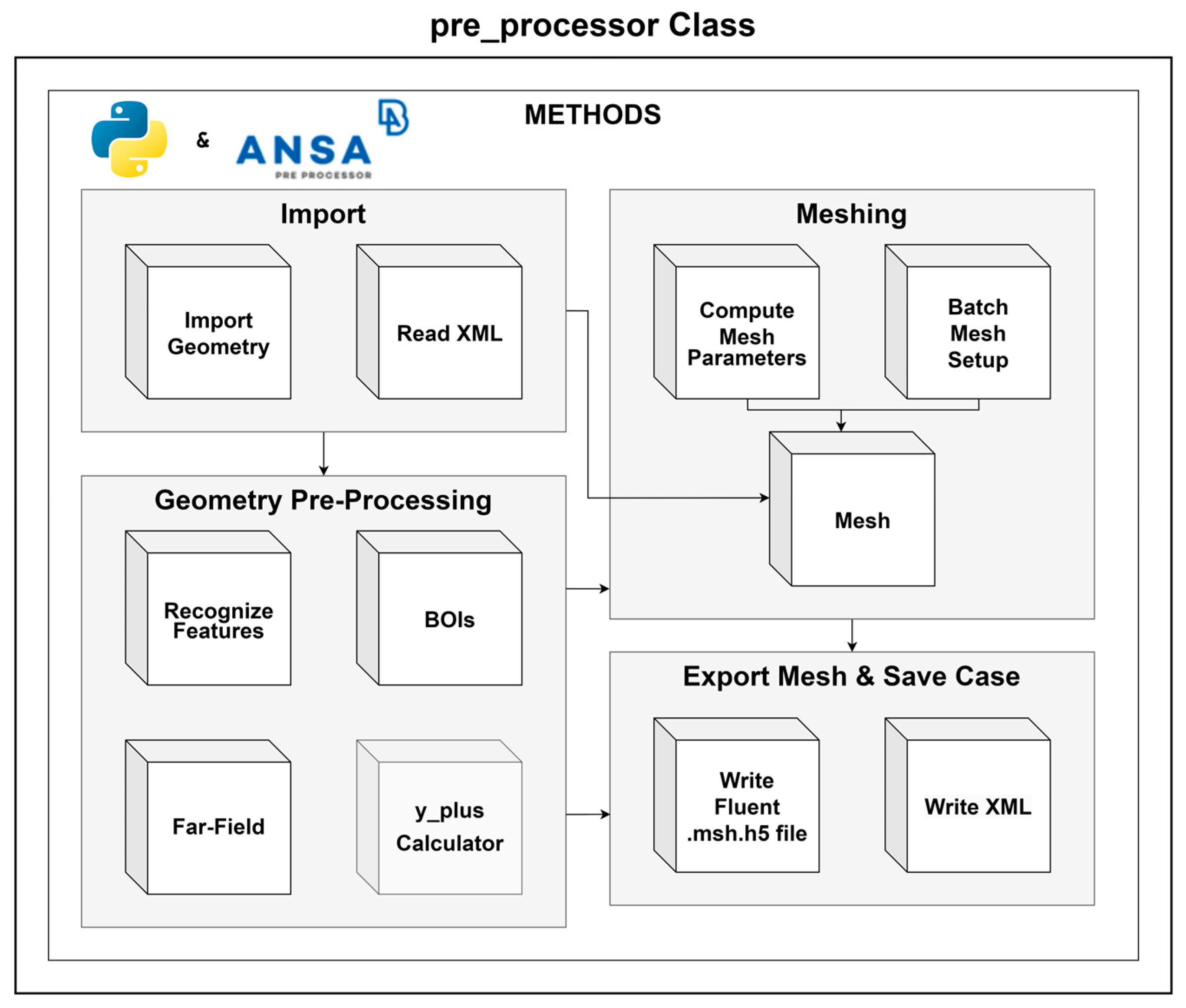
3.2. Mesh Module

The mesh module bridges the gap between raw geometry and solver-ready computational meshes. This module is tasked with two primary objectives: geometry pre-processing and mesh generation. The first objective builds upon the modeled wing generated by the geometry module, performing geometric manipulations to prepare a watertight control volume for mesh generation. This includes steps such as feature recognition, body of influence (BOI) definition, and far-field boundary creation. These steps are further analyzed and discussed in Appendix A.2 and Appendix A.3.

The second objective (mesh generation) involves discretizing the computational domain into smaller cells or elements, which act as control volumes for solving the governing equations of fluid flow. The quality of the mesh directly impacts numerical accuracy, numerical stability, and computational efficiency, as it determines the resolution of key physical phenomena such as boundary layers, wake regions, and separation zones.

Implemented via the ANSA Python API, the module uses an object-oriented pre_processor class with four method categories, as illustrated in Figure 6. The process begins with import methods, which handle the data transfer from the geometry module, importing STEP files and extracting attributes from the XML file for a case-specific setup. Next, feature recognition is performed to identify critical regions such as leading edges, trailing edges, and sharp perimeters. Bodies of Influence (BOIs) are then defined, along with the far-field boundaries of the computational domain. Following these geometric pre-processing steps, the meshing operations take place. Mesh parameters are dynamically adjusted using the custom Compute_Mesh_Parameters method and the geometric attributes of the given wing. The custom Batch_Mesh_Setup method then updates the meshing sessions/scenarios before generating the mesh in the following sequence: (1) surface meshing for both the wing wall and the far-field boundaries, (2) inflation layer mesh, and finally (3) volume meshing. Finally, the Export Mesh and Save Case methods save the mesh in Fluent-compatible .msh.h5 format and generate XML files for case tracking and attribute documentation.

At this stage, one notable feature of the XML file becomes evident: it serves as a bridge between the modules by enabling the transfer of all attributes and data from the Wing class to the pre_processor class. This eliminates the need for direct serialization, streamlining data handling within the framework. Once the geometry generation step is complete, the XML file ensures that the meshing module can independently proceed at a later time without requiring direct interaction with the geometry module.

3.2.1. Meshing for CFD

Selecting the appropriate meshing criteria depends on the geometric complexity, flow conditions, and the desired level of simulation fidelity. Different mesh types—categorized as structured, unstructured, or hybrid—each offer distinct benefits and challenges. Structured grids, characterized by their uniform and ordered connectivity, are highly efficient and accurate for simple geometries and flow-aligned features [43]. However, their rigid structure makes them challenging to apply to complex or multi-element configurations. Unstructured grids, on the other hand, provide flexibility to adapt to highly irregular geometries, covering intricate features like sharp edges or highly curved surfaces. Hybrid grids combine the advantages of both, employing structured grids in regions where precision is important, and unstructured grids in less critical areas.

In this work, the hybrid mesh approach is selected. A structured curvilinear mesh (inflation layer) is employed over the boundary layer region to capture critical near-wall phenomena, while for the remainder of the domain, an unstructured grid is chosen to flexibly adapt to the overall geometry. As for discretization elements, hexahedrals are predominantly used for both boundary layers and far-field regions, as they offer superior numerical accuracy and alignment with flow gradients [41].

Considering the practical implementation, the mesh of any arbitrary wing within the framework is generated via custom meshing scenarios which are passed through the ANSA batch mesh tool. These scenarios are tailored by parametrizing meshing options with the wing’s geometric characteristics, as observed in

Table 4. Parameters that control surface mesh.

		Wing-Wall Session	Wingtip Session	Far-Field Session
Mesh type	Algorithm	CFD	CFD	CFD
	Element Type	Quads and Trias	Quads and Trias	Quads and Trias
	Order	1st	1st	1st
Mesh Sizing	Growth Rate	1.2	1.2	1.2
	Max Length	$f\left(MAC\right)$	$f\left(c_3\right)$	$f\left(c_1\right)$
Curvature Refinement	Distortion Angle	0	0	15
	Min length	$f\left(c_3\right)$	$f\left(c_3\right)$	-
Leading Edge Treatment	Distribution	Anisotropic	-	-
	Min first height	$f\left(c_3\right)$
	Growth Factor	1.15
	Max Aspect	1
Trailing Edge Treatment	Distribution	Anisotropic	-	-
	Min Aspect	0.05
	Growth Factor	1.15
	Max Aspect	0.7
Sharp Edge Treatment	Max Length	-	$f\left(c_3\right)$	-

. The meshing module operates autonomously, requiring no additional user inputs. The batch mesh tool for CFD applications usually requires a surface meshing scenario, an inflation layer scenario, and a volume-meshing scenario. Each meshing scenario consists of multiple meshing sessions, addressing different aspects of the geometry. Specifics considering the meshing scenarios, the meshing parameters, and special treatments are discussed in Appendix A.3.

3.2.2. Surface Mesh

The shaded fields in Table 4 represent meshing parameters that are directly parametrized using geometric inputs specific to the wing’s design. These parametrizations are chosen with guidance from the established literature and reflect best practices to ensure computational accuracy and efficiency. For instance, the “minimum length” under “curvature refinement” and the “minimum first height” in “leading edge treatment” share a value of approximately 0.1% of the tip chord. Consistent with guidelines from the literature, refining key areas, such as leading and trailing edges to approximately 0.1% of the chord length and ensuring 80–100 cells along the chordwise direction, enhances the resolution required for capturing curvature effects and boundary layer dynamics [41]. Additionally, anisotropic distribution and gradual growth factors in mesh elements are recommended for resolving high-gradient regions near walls [43]. Other mesh parametrizations are derived by trial and error while testing the limits of the design space and grid independence studies that are mentioned in Section 5.1.

The automatic control over mesh sizing is achieved through .ansa_mpar files, which are edited automatically and passed to the ANSA pre-processing software. The .ansa_mpar files are configuration files that specify mesh parameters for different regions of a geometry. Each meshing session corresponds to an ansa parameter file. The modification of the .ansa_mpar files is achieved via the ansa_mpar_file_editor module, a custom utility developed to automate the process of editing these files. This module enables dynamic adjustments to mesh parameters by leveraging Python’s file-handling capabilities and regular expressions to target specific configuration settings within .ansa_mpar files. The modification of .ansa_mpar files is performed during the call of the compute_mesh_parameters, a custom method included in the pre_processing class.

3.2.3. Inflation Layer Mesh

This study employs a wall-resolving approach to accurately capture near-wall phenomena, which are critical for predicting aerodynamic characteristics. The near-wall region is dominated by the boundary layer, transitioning from the viscous sublayer dominated by laminar flow, where fluid particles move in orderly layers, to turbulent flow, characterized by chaotic fluctuations. These transitions significantly affect performance metrics such as skin friction and separation zones, making precise boundary layer modeling a necessity [44,45].

To address these challenges, the near-wall treatment focuses on resolving flow structures adjacent to the wall, guided by the non-dimensional wall distance $y^{+}$ [46]. Depending on the turbulence modeling approach, the meshing strategy ensures the first cell lies at a specific $y^{+}$, which in CFD applications is called first-layer $y^{+}$, or simply $y^{+}$. As mentioned at the beginning of Section 3, this study employs the k-omega SST turbulence model [38]. Considering the latter, grid refinements target average $y^{+}$ values less than one ($y^{+}<1$), which is essential for resolving the viscous sublayer.

The ANSA software allows us to have more control over specific features of the inflation layer; these features are listed below.

• The first two layers are of the same height, equal to the first layer height calculation discussed in Appendix A.3.
• A growth factor is applied for a specific number of layers that are calculated according to the total boundary layer height (see Appendix A.3).
• To ensure the full coverage of the physical boundary layer and a smooth transition from the inflation layer to the volume mesh, additional layers are added on top for redundancy.

The inflation layer height is calculated iteratively, starting with an initial thickness of twice the first layer height. Successive layers are generated using a growth factor, typically set to $1.2$ for smooth transitions. The iterative process continues until the total inflation thickness equals or exceeds the estimated boundary layer thickness ($\delta$). When the total inflation thickness exceeds the flat plate boundary layer height, the number of layers is returned and adjusted by a safety factor ($1.1$) to ensure adequate coverage, according to suggested practices [41]. Finally, additional layers are placed on top for redundancy. 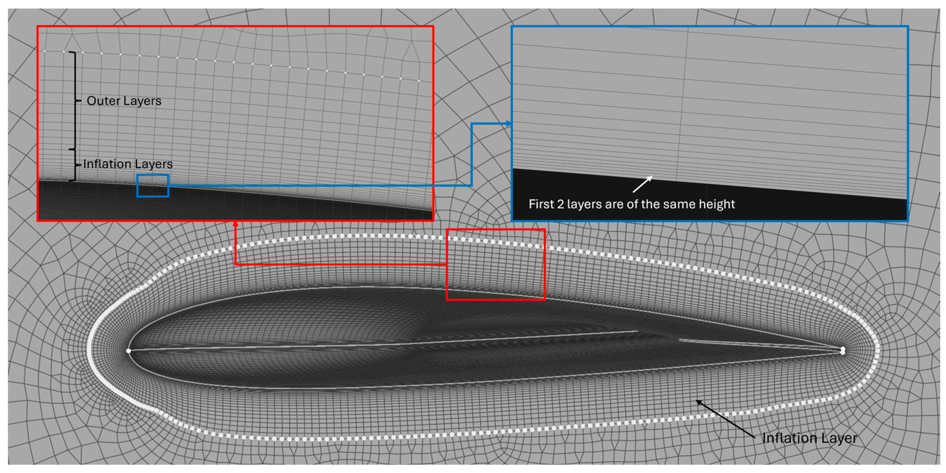The following inflation layer (Figure 7) is produced automatically using the proposed framework.

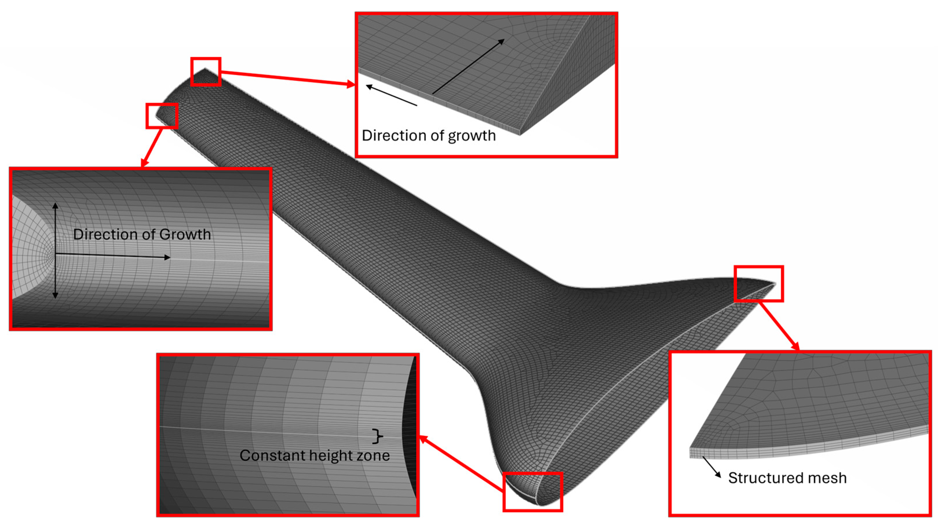
The zoomed-in views in Figure 7 highlight critical aspects of the grid structure at the symmetry plane. The right view focuses on the inflation layers, showing finely spaced layers adjacent to the body, with the first two layers being the same height. The left view shows the transition from the inflation layers to the additional layers and then the outer grid, where 10 coarser layers extend to the outer domain. Note that the inflation layer growth factor also applies to the outer layers, which are added as a safety cushion. This ensures that the region of the actual boundary layer will always fall in this curvilinear structured grid.

3.2.4. Volume Mesh

Volume meshing is the final step during the mesh generation process, generating elements in the space between the inflation layer top cap and the far-field boundaries. The utilized volume-meshing algorithm produces an unstructured grid of hexahedrals wherever possible, and tetrahedrals (pyramids) in places where hexas are not allowed. For consistency, the meshing algorithm is called “HexaPoly”.

3.3. Solver Module

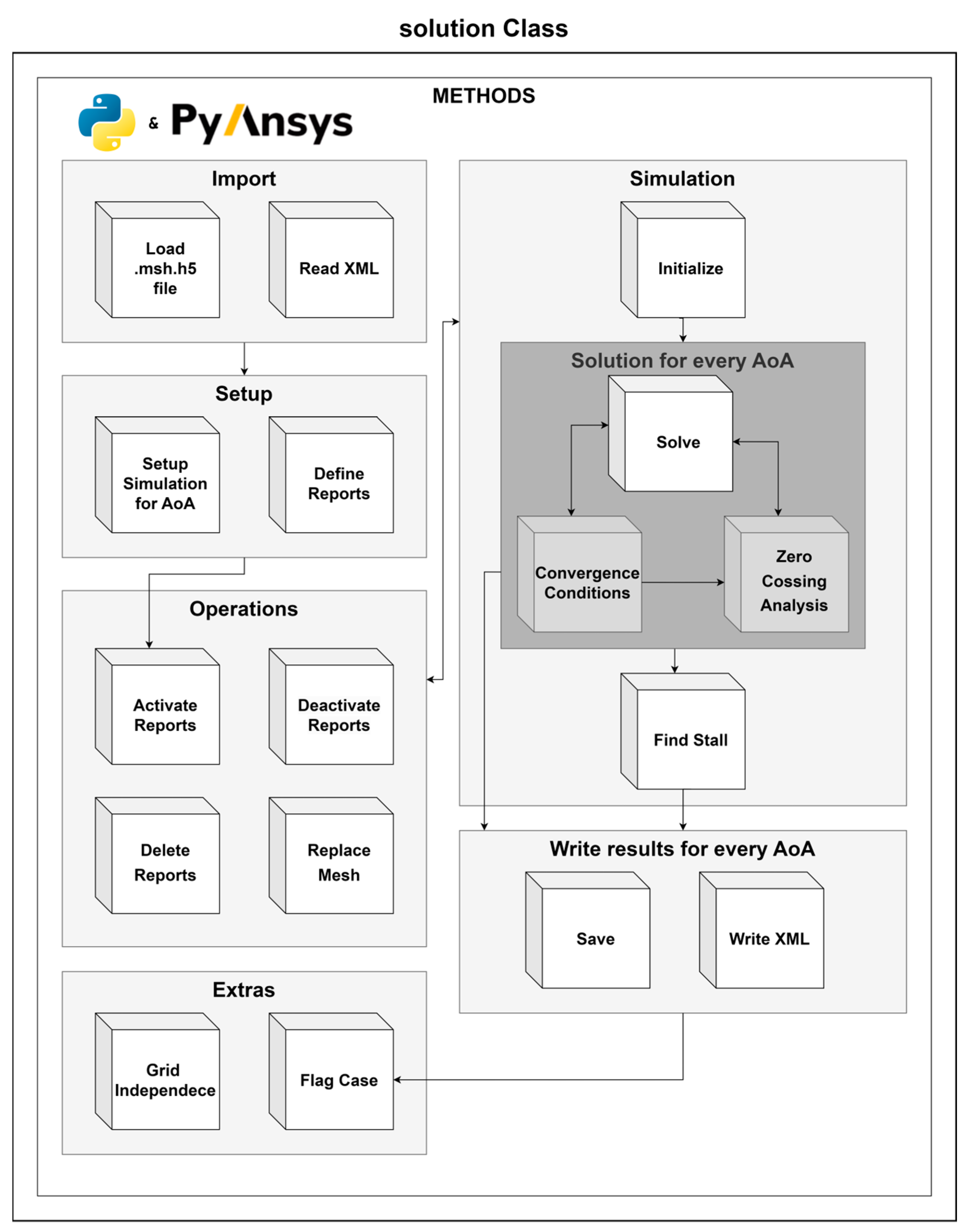
The solver module integrates ANSYS Fluent 2023R2 via PyFluent to automate simulation setup, execution, and post-processing. Utilizing Fluent’s GPU-native solver, calculations achieve up to 7× faster computational times compared to parallel CPU solvers, significantly reducing simulation duration [47]. A dedicated solution class, illustrated in Figure 8, manages input and output files, simulation setup, and execution. It also supports stall detection and convergence monitoring methods, ensuring high-fidelity results with minimal manual effort.

To initiate this process, instantiating the solution class also launches Fluent automatically according to the specified launcher settings. Whether running in GPU or CPU mode, with or without GUI, and using a predefined number of processors, the solver is initialized with the appropriate computational resources before proceeding with the case setup and execution.

Once Fluent is up and running, the module proceeds with loading the computational mesh from a .msh.h5 file. It then parses the XML file, extracting previously calculated attributes, including the MAC, reference surface area, Reynolds number, velocity, and altitude. These values are utilized in defining the simulation’s boundary conditions and reference parameters for later force and moment calculations.

The simulation setup is then performed iteratively over a predefined range of angles of attack. For each AoA in the range, the class executes all setup procedures detailed in Appendix A.4. Monitoring report files for lift, drag, and moments are also generated during the simulation, providing real-time feedback on solution convergence and stability. After initializing the solution, the simulation then enters an iterative solution phase, where Fluent runs for a predefined number of iterations while continuously checking for convergence, as described in Algorithm for Convergence Detection section. Once the solver detects convergence, the aerodynamic coefficients $C_L$, $C_D$, and $C_M$ are computed using the final force and moment values. Post-processing includes extracting maximum and mean $y^{+}$ values to evaluate the quality of the boundary layer resolution. The final results are stored in the XML file, and Fluent’s output files (.cas.h5, .dat.h5, .out) are also saved.

Throughout this process, robust error handling mechanisms ensure that Fluent automatically retries execution or logs issues if it encounters errors such as failed launches or missing files. The class is designed to efficiently manage multiple cases, automating the CFD workflow.

Algorithm for Convergence Detection

In CFD, convergence refers to the stabilization of iterative calculations of flow variables, indicating that the numerical solution is approaching a state that sufficiently satisfies the governing equations and boundary conditions. Typically, convergence is judged by a three-order-of-magnitude drop in residuals of continuity, momentum, and turbulence equations, alongside the stabilization of forces such as lift and drag [48]. Achieving convergence to machine precision is realistically impossible, and practical thresholds must balance accuracy and computational cost.

In this framework, a custom convergence detection algorithm is implemented due to the limitations of Fluent’s built-in methods for GPU-native solvers (Fluent v2023R2—v2024R2). This algorithm is incorporated as a hidden method within the solution class and called by the solve method while a simulation is running. This dependency can be observed in Figure 4 and Figure 8. The method incorporates residual monitoring, periodicity checks, and termination criteria, focusing specifically on the aerodynamic quantities of interest: the forces acting along the $x$ and $z$ axes. The residual of these forces is calculated iteratively as the maximum relative change in force values over a specified window of past iterations ($N$), using the formula of Equation (1).

$$R_{F_{x,z}}^{\left(i\right)}=\underset{N}{\max }\left({\displaystyle \frac{\left|{F^{\left(i\right)}}_{x, z}-{F^{\left(i-j\right)}}_{x, z}\right|}{\left|{F^{\left(i\right)}}_{x, z}\right|}}\right)$$

(1)

Note the following:

$R_{F_{x, z}}^{\left(i\right)}$: Maximum residual force in the $x$ or $z$ direction at iteration $i$;

$F_{x,z}^{\left(i\right)}$: Current force in the $x$ or $z$ direction at iteration $i$;

$F_{x,z}^{(i-j)}$: Force value in the $x$ or $z$ direction from $j$-th previous iteration.

Residual convergence is flagged when both forces drop below a predefined residual flag for three consecutive checks, performed at specified iteration check interval. Periodicity detection, initiated after a defined iteration threshold and a defined level of convergence (residual flag should be at least as low as one order of magnitude larger than the threshold), uses zero-crossing analysis to identify stable oscillatory behavior [49]. If periodicity is confirmed, the solution is conditionally converged. Additionally, a maximum iteration cap of 2000 iterations is imposed to prevent excessive computational costs in scenarios where convergence or periodicity detection cannot be achieved. In those cases, the evaluation metrics described in Section 4 can assist in investigating the convergence issue.

Based on the findings of a sensitivity study, combining a ${10}^{-3}$residual flag, 100-iteration checking window, and 10-iteration check interval is suggested as a balanced trade-off between computational cost and convergence robustness. The approach ensures high reliability and robustness in detecting convergence, accommodating the complexities of GPU-native solvers and aerodynamic flows.

4. Evaluation Metrics

The reliability of CFD results must consider the quantification of numerical errors, especially in an automated framework where human intervention is minimized. Thus, it is essential to ensure that the solutions generated are accurate, especially when considering critical aerodynamic quantities like lift and drag. The error in CFD modeling can be categorized into round-off errors, discretization errors, and iterative errors [50,51,52].

• Round-off errors arise from the finite precision of numerical calculations performed by computers, particularly in large-scale simulations with many iterations, where the accumulation of small errors can impact the solution.
• Discretization errors, on the other hand, result from the approximation of continuous governing equations using numerical schemes and finite spatial or temporal resolution. They encompass truncation errors, which arise from the omission of higher-order terms in the numerical approximation, and additional artifacts introduced by grid quality, boundary condition definition, and numerical schemes. Discretization errors are often treated as an epistemic uncertainty [53], reflecting incomplete knowledge of the true solution due to mesh and scheme limitations.
• Iterative errors stem from the incomplete convergence of the solver to a stable solution, either due to insufficient iterations or suboptimal solver settings, and are similarly treated as an epistemic uncertainty [54].

While these errors cannot be entirely eliminated, estimating their impact is essential for assessing the numerical fidelity of CFD results. Such error estimation safeguards against misinterpreting numerical artifacts as physical phenomena and helps ensure that the automated workflow produces robust and reliable outputs.

To complement the error estimation process, this study also introduces a rapid reliability assessment methodology for evaluating the overall quality of CFD results. This assessment uses established best practices and guidelines for CFD simulations in the subsonic regime [41,48]. By systematically evaluating critical parameters—such as boundary layer resolution, the number of discretized cells within the boundary layer, and the convergence behavior of key forces—the methodology identifies unreliable simulations and highlights potential sources of inaccuracy. These quality checks act as a double-layer safeguard, ensuring that the solutions meet predefined standards of fidelity before progressing further in the design process.

Together, error estimation and rapid reliability assessment form a comprehensive framework for validating CFD outputs. The framework not only quantifies numerical uncertainties but also ensures solution quality through practical and experience-based reliability checks. This dual approach provides designers with robust and reliable outputs, enabling informed decision-making during the design and optimization process.

4.1. Discretization Error Quantification

This subsection focuses on two primary error sources: the Grid Convergence Index (GCI), which quantifies discretization errors, and iterative errors, which arise from incomplete solver convergence. These methods allow for the estimation of numerical uncertainties, enhancing confidence in the CFD solutions.

The Grid Convergence Index (GCI), rooted in Richardson extrapolation, is a well-established method for estimating discretization error in CFD simulations, while it has been validated against experimental data across diverse aerodynamic applications [55]. The GCI evaluates the convergence of key aerodynamic quantities, such as lift and drag, across systematically refined grids. The procedure is as follows:

• Define a Representative Grid Size: for three-dimensional grids, Equation (2) is used.

  $$h={\left[{\displaystyle \frac{1}{N}}\sum _{i=1}^N{\mathrm{V}}_{\mathrm{i}}\right]}^{{\displaystyle \frac{1}{3}}}$$

  (2)

Note that $V_i$ is the volume of the $i_{th}$ cell and N is the total number of cells.

2.

Grid Refinement: perform analyses on three grids (coarse, medium, and fine), characterized by grid sizes $h_1<h_2<h_3$, with a refinement ratio $r$ (Equation (3)).

$$r={\displaystyle \frac{h_{coarse}}{h_{fine}}}>1.3$$

(3)

3.

Apparent Order of Accuracy p: Calculate p using Equations (4)–(6).

$$p={\displaystyle \frac{1}{\mathrm{l}\mathrm{n}\left(r_{21}\right)}}\left|\ln \left({\displaystyle \frac{{\phi }_3-{\phi }_2}{{\phi }_2-{\phi }_1}}\right)+q(p)\right|$$

(4)

$$q\left(p\right)=ln\left({\displaystyle \frac{r_{21}^p-s}{r_{32}^p-s}}\right)$$

(5)

$$s=1\times sgn\left({\displaystyle \frac{{\phi }_3-{\phi }_2}{{\phi }_2-{\phi }_1}}\right)$$

(6)

In these equations, φ is the aerodynamic quantity of interest. The equations for p can be solved using fixed-point iteration.

4.

Extrapolated Solution: Use Richardson extrapolation (Equation (7)) to approximate the solution at an infinitely fine grid.

$${\phi }_{ext}^{21}={\displaystyle \frac{r_{21}^p{\phi }_1-{\phi }_2}{r_{21}^p-1}}$$

(7)

5.

Discretization Error (GCI): The error estimates are reported (Equations (8) and (9)).

$$\begin{gathered} {\epsilon }_{31}=\left|{\displaystyle \frac{{\phi }_3-{\phi }_1}{{\phi }_1}}\right| \\ {\epsilon }_{3,ext}=\left|{\displaystyle \frac{{\phi }_3-{\phi }_{ext}^{21}}{{\phi }_{ext}^{21}}}\right| \end{gathered}$$

(8)

$$GC{I}_{fine,31 }=1.25{\displaystyle \frac{{\epsilon }_{a,31 }}{r_{31}^p-1}}$$

(9)

4.2. Iterative Error Quantification

Iterative errors arise due to the non-linearity inherent in the governing equations, such as the Reynolds-Averaged Navier–Stokes (RANS) equations, and the iterative nature of numerical solvers [52,56]. Non-linearities from convective terms, turbulence closure models, and deferred corrections in discretization contribute significantly to iterative errors. Additionally, the solution of linearized algebraic systems through iterative methods introduces convergence-related discrepancies. While iterative errors can be reduced with additional iterations, achieving complete convergence is often computationally prohibitive, particularly in complex turbulent flows. This necessitates the adoption of reliable methods to quantify and manage iterative errors within acceptable limits to ensure the fidelity of CFD simulations.

Despite significant advancements in CFD, iterative errors remain an open problem, with numerous studies endeavoring to address their impact and quantification [50,51,52,55,56]. The approach to iterative error estimation employed in this study aligns with the same study utilized for the discretization error, thereby ensuring consistency and credibility within the numerical uncertainty framework. In this context, iterative error fulfills a dual role. It serves as a practical indicator of convergence, enabling engineers to assess whether a solution has stabilized by closely monitoring the error as the solution progresses. Furthermore, it provides an approximation of uncertainty, allowing for the estimation of numerical error should the simulation be terminated prematurely.

To quantify the iterative error, the methodology proposed by Ferziger [57] is employed. The iterative error, denoted as ${\mathsf{\epsilon }}_{iter}$, is estimated using the formula of Equation (10).

$${\epsilon }_{iter,i }^n\cong {\displaystyle \frac{\left({\phi }_i^{n+1}-{\phi }_i^n \right)}{{\lambda }_i-1}}$$

(10)

Note that $n$ is the iteration number, ${\phi }_i$ is the solution variable, and ${\lambda }_i$ is the principal eigenvalue of the solution matrix, approximated using Equation (11).

$${\lambda }_i={\displaystyle \frac{‖{\phi }_i^{n+1}-{\phi }_i^n‖}{‖{\phi }_i^n-{\phi }_i^{n-1}‖}}$$

(11)

The uncertainty in iteration convergence, ${\delta }_{iter}$, is then calculated as shown in Equation (12).

$${\delta }_{iter}={\displaystyle \frac{‖{\epsilon }_{iter,i}^n‖}{{\lambda }_{ave}-1}}$$

(12)

In this equation, ${\lambda }_{ave}$ is the average value of ${\lambda }_i$ over a reasonable number of iterations. Following recommendations in prior studies, ${\lambda }_{ave}$ is calculated using 1% of the total iterations [51].

4.3. Solution Confidence

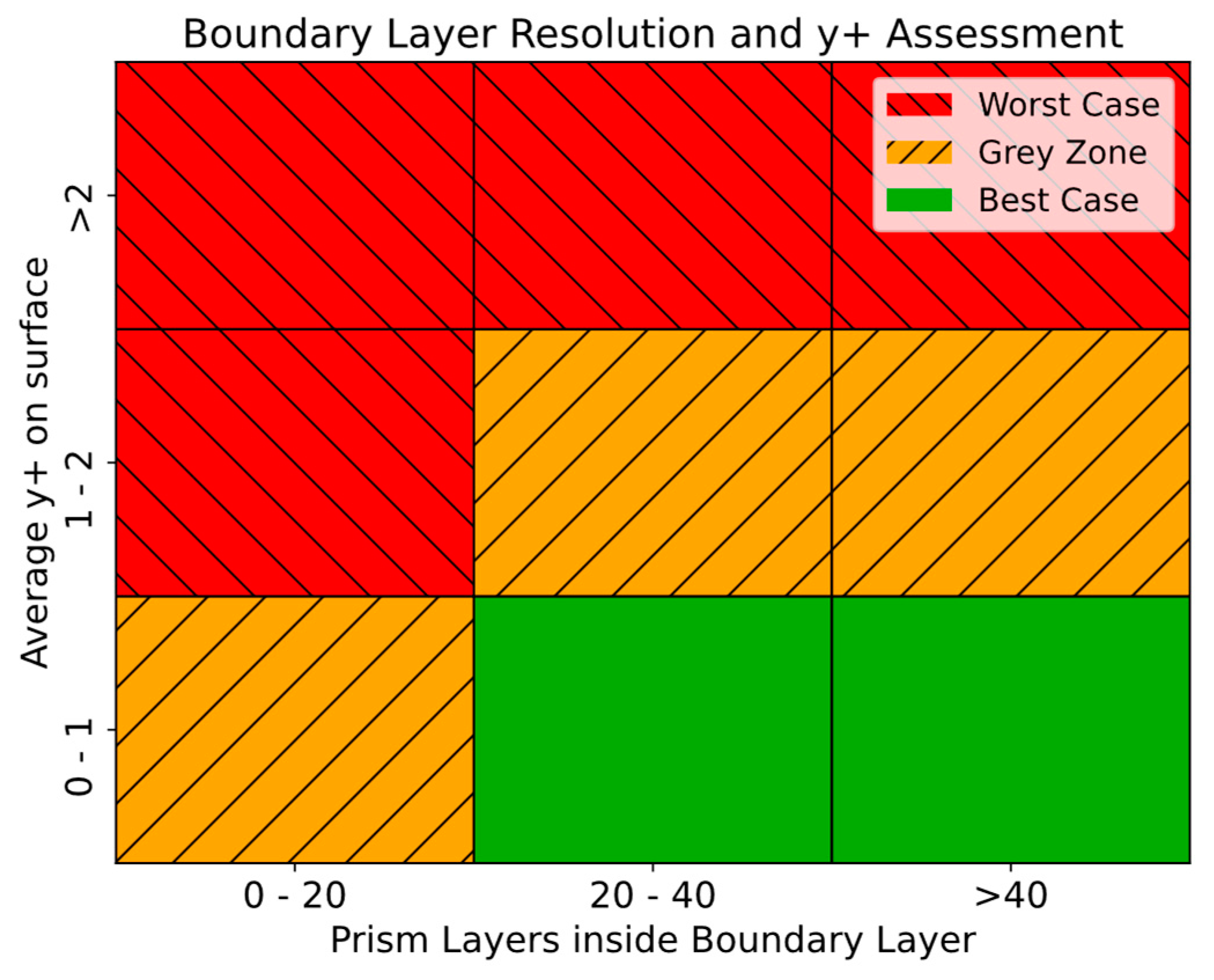
Unlike global error estimates, key simulation quality indicators provide a practical and immediate assessment of grid and solution reliability. The confidence metrics utilized in this study are systematically implemented as part of the automated process, providing a quick and actionable diagnostic tool to assess simulation quality. By flagging runs that deviate from established thresholds, this method empowers engineers to either proceed with confidence or refine their setup, thus safeguarding the integrity of the design process.

According to widely accepted guidelines for the subsonic regime, as well as experimental validations [58], proper resolution of turbulence effects—particularly when using the low-Reynolds variant of the k-omega SST turbulence model adopted in this study—requires careful treatment of the boundary layer grid. For accurate turbulence modeling and wall shear stress prediction, an average $y^{+}$ value of less than 1 and a maximum $y^{+}$ value of 2 should be enforced across the wing surface. While a maximum $y^{+}$ value strictly below 1 is suggested by some researchers (see

Table 5. Proposed $y^{+}$ values and prism layers in boundary layers in different studies.

Study	$\mathbf{Proposed} {\mathit{y}}^{+}$	Proposed Prism Layers
Menter et al., 1994 [38]	3	N/A
Georgiadis et al., 1995 [58]	2	N/A
Menter et al., 2015 [59]	1	30
Goetten et al., 2019 [41]	N/A	20–40
Menter et al., 2003 [60]	2	N/A
ANSYS–Menter 2021 [48]	1	30–40

) as an ideal target, it is often unrealistic to achieve this consistently in automated frameworks, especially when considering the broad design space and flow conditions investigated in this work.

Nevertheless, it should be noted that this practical guideline is applied to ensure that the low-Reynolds modeling will consider the phenomena encountered within the viscous sublayer, which appears at a $y^{+}$ smaller than 5 [46].

Several studies have attempted to quantify the sensitivity of aerodynamic quantities to variations in $y^{+}$ values across a range of geometries and flow conditions [58,59]. However, these efforts remain limited, both in scope and applicability, as they do not comprehensively cover the design space or operational conditions explored in this study. As such, relying solely on $y^{+}$values for a quantified grid-resolution error remains impractical and, in many cases, misleading.

In addition to satisfying the first layer height requirements near wall boundaries, an accurate boundary layer resolution also demands a sufficient number of prism layers within the boundary layer to properly capture the flow phenomena starting from the near-wall region of the viscous sublayer and moving on to the buffer zone and logarithmic region. Existing studies have established that 20 to 40 prism layers are typically required to discretize the boundary layer accurately and ensure numerical fidelity (see Table 5). This ensures that steep gradients, particularly in the near-wall regions, are resolved with an adequate grid density.

By combining the guidelines for $y^{+}$ and the boundary layer discretization, a systematic confidence assessment system is suggested in the current study, indicatively using color coding to flag deviations from established thresholds. This system allows for a rapid visual evaluation of simulation reliability, as illustrated in Figure 9.

The green color represents the best-case scenario according to most guidelines, the orange color (left cross pattern) represents a type of grey zone where some studies agree, and the red color (right cross pattern) indicates poor confidence about the results of the analysis. In this framework, the $y^{+}$ values (both average and maximum) are extracted using the solver module and the functionality provided by PyFluent, utilizing built-in methods.

A critical factor contributing to the confidence in the results is the convergence behavior of each case. As described in Section 3, a substantial computational budget is allocated to the solution, and an automated algorithm continuously monitors the quantities of interest (forces generated on the wings) until they stabilize within a predefined tolerance level. Cases that fail to converge may indicate oscillatory or divergent behavior, or, in rare instances, a very slow rate of convergence, as observed in the authors’ experience. For every CFD result, the convergence condition is reported alongside the residuals for each force, providing designers with valuable insights into the simulation setup.

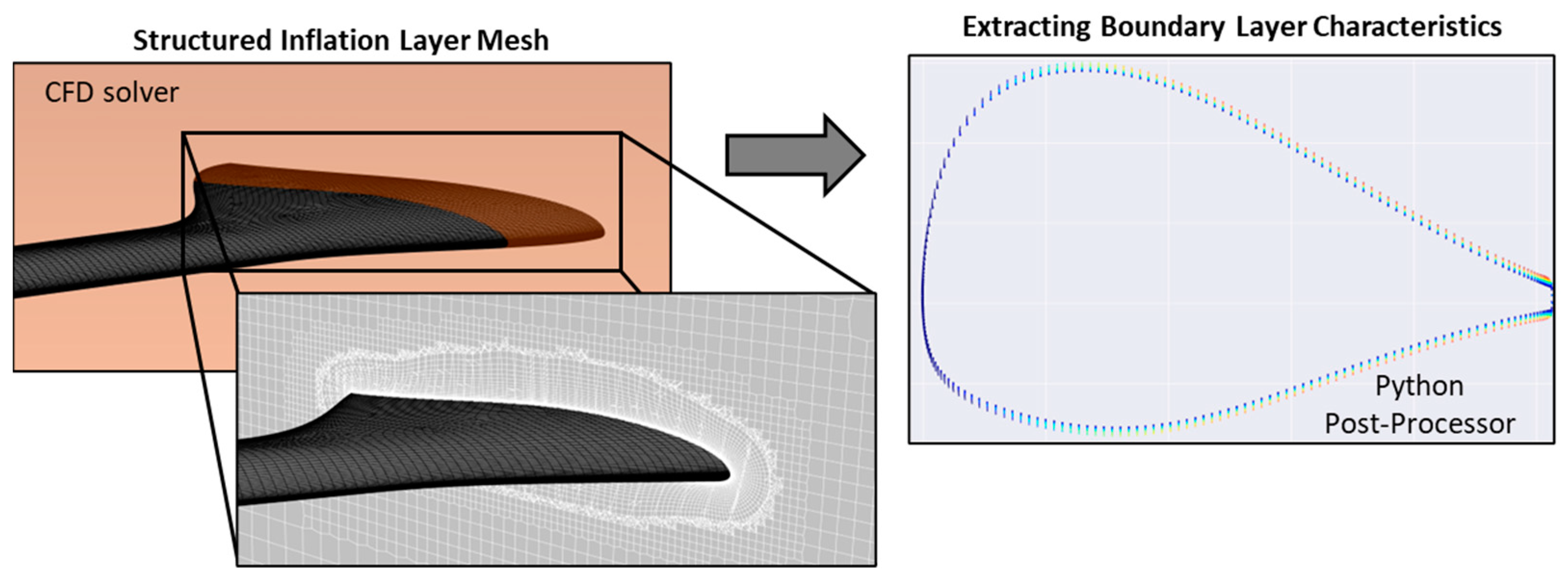
Inflation Layer Exploration

This section and Figure 10, describes the approach adopted to generate a structured inflation layer mesh from unstructured CFD simulation data with the scope of accurately defining the grid elements inside the boundary layer (Figure 11). The development of a structured inflation layer mesh, while complex, enables the detailed post-processing of these regions.

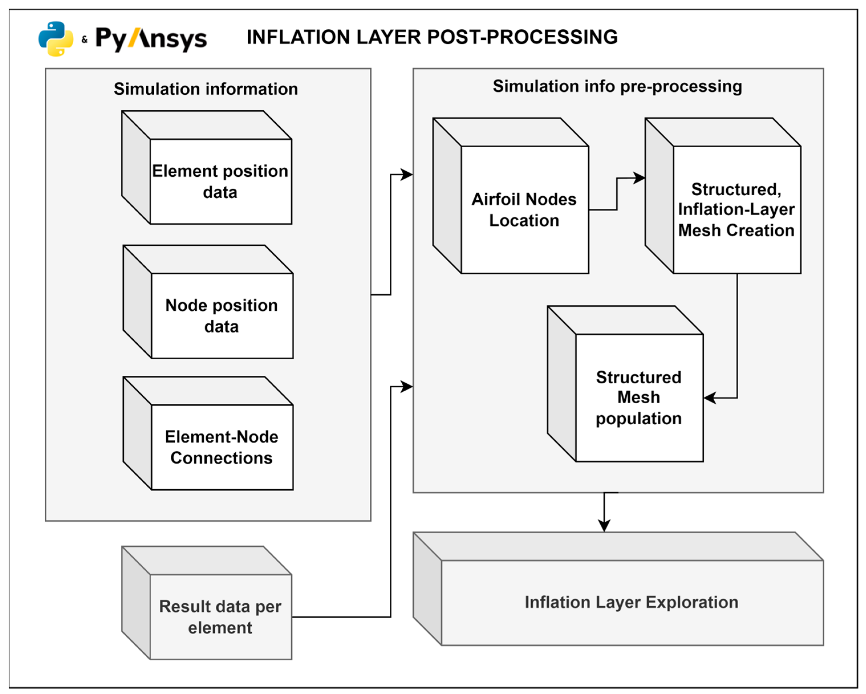
The initial step involves extracting the simulation data, including element positions, node positions, and element–node connectivity. This information is gathered via PyFluent and forms the foundation for mapping relationships between nodes and elements, which is necessary for reconstructing structured layers. The data structure allows for the efficient traversal and identification of edges shared between elements, enabling the formation of a coherent network around the airfoil. The airfoil boundary is located by identifying nodes lying along its surface. These nodes are determined based on their spatial arrangement (their proximity to the plane of interest), their velocity magnitude (which should be zero according to the no-slip boundary condition imposed), and distinct geometric features, such as proximity to the airfoil shape and minimal deviation in the tangential direction. Once identified, the airfoil nodes are chained into a continuous sequence, representing the airfoil surface from the leading edge to the trailing edge. This chaining process preserved the geometric coherence of the airfoil outline.

Subsequently, elements connected to the airfoil nodes are isolated, using the connection information from the solver, forming the first inflation layer directly adjacent to the airfoil. The elements are ranked based on their proximity and connectivity to ensure an unambiguous representation of the layer.

Using the elements of the first layer as a foundation, additional inflation layers are constructed incrementally. For each layer, the following process is applied:

• Element Connectivity Traversal: The neighboring elements of the current layer are identified through their shared edges.
• Velocity and Y-Coordinate Filtering: Candidate elements for the next layer are filtered based on predefined constraints on x-velocity component and vertical (z-axis) alignment, ensuring physical relevance.
• One-to-One Mapping: A one-to-one mapping is enforced between elements of consecutive layers to maintain coherence. This ensured that each element in a new layer corresponded to exactly one element in the previous layer, preserving the structured arrangement.
• Continuity Validation: Additional continuity checks ensured the spatial arrangement of elements remained consistent. A maximum allowable distance criterion was applied between consecutive elements to detect and resolve discontinuities.

With the structured data array, including computed variables such as the fluid velocity and turbulent viscosity ratio, the boundary layer height can be determined at any position along the airfoil [48,61]. This enables a direct comparison with theoretical boundary layer heights and allows for the counting of prism cells within the boundary layer. While this proposed methodology shows promise for automatically extracting boundary layer information, its application is limited by the strong three-dimensional effects arising from varying boundary layer development rates along the wing. Consequently, constructing concise metrics to inform designers is beyond the scope of this study. However, the method can still be applied manually by selecting specific points of interest on the wing surface.

5. Framework Performance

The performance evaluation of the proposed framework is conducted through a combination of validation studies and a large-scale development in order to acquire statistical insights across a large sample of the design space. Firstly, in Section 5.1, a grid independence study is conducted alongside the quantification of discretization errors in the generated grids. It must be noted at this point that the main goal of this work is to present and demonstrate the entire pipeline of a framework that leads from geometry to simulation. Validating the framework against experimental or flight-testing data is beyond the scope of this work, especially given the fact that the methods have been validated in previous studies in their non-automated form. Additionally, in Section 5.2, a validation case is selected to benchmark the framework’s performance against the expertise of a highly skilled mechanical engineer specializing in CFD. This comparison focused on both time efficiency and the accuracy of the results.

Following this, in Section 5.3, an extensive series of analyses were conducted, sampling 1165 wings from the predefined design space (Section 2). The purpose of these analyses is to assess the framework’s performance across four primary aspects:

(1)

sampling a range of wing configurations;

(2)

meeting boundary-layer resolution and mesh-quality thresholds (Section 4);

(3)

ensuring solver convergence and minimal iterative error;

(4)

achieving computational efficiency for large-scale design exploration.

The findings indicate that the framework can handle a wide range of wing configurations without user intervention, while also providing detailed information on computational durations for geometry generation, mesh generation, solution setup, and solution execution. Additionally, the grids generated were evaluated using the quality metrics described in Section 4.

All the analyses presented in this section for the framework’s performance are conducted at the Aristotle University of Thessaloniki (AUTh) High Performance Computing (HPC) cluster, leveraging its advanced computational capabilities. This state-of-the-art system facilitated the efficient execution of the large-scale simulations required for validating the framework and analyzing the sampled wings. The HPC cluster specifications are detailed in

Table 6. AUTh’s system cluster specifications.

Component	Quantity	Specification
CPU Cores	16	AMD EPYC 7742
GPU	1	NVIDIA A100 40 GB
RAM	128	Gb of DDR4

.

It should be noted that the definition of a “highly skilled Mechanical Engineer specializing in CFD” is inherently subjective. In this case, the expert is an engineer with over five years of experience in CFD, specifically for aircraft and UAV applications [39,62,63,64]. The expert has served as the lead CFD engineer on multiple research and industrial projects, developing expertise in aerodynamic analysis, mesh optimization, and simulation validation. While this level of expertise provides a solid benchmark for comparison, it is acknowledged that individual skill sets and methodologies can vary significantly across practitioners, which may influence the comparison outcomes.

5.1. Grid Independence Studies and Error Quantification

This section focuses on performing grid independence studies within the framework, ensuring that the solution converges under mesh refinement using previously established practices [39]. Because these studies are performed by the framework automatically, the simulation setup, including model and solution scheme selection, matches the setup detailed in Algorithm for Convergence Detection section.

The ONERA M6 wing is selected for the grid independence studies due to its simplicity, public availability, and frequent use in benchmarking studies [65]. This well-documented geometry, depicted in Figure 12 is a staple in aerodynamic validation, offering established reference data for comparison. Although the ONERA M6 wing is commonly validated in high-speed subsonic and transonic flow regimes, this study is focused on subsonic incompressible flow conditions. Transonic regimes demand more intricate grid setups and solver configurations, which are outside the framework’s intended operational domain [66]. The ONERA M6 model, along with the corresponding design space parametrization, is illustrated in Figure 12 and

Table 7. Parametrization of the ONERA M6 wing.

Parameter	ONERA M6
$c_1$	805.9 mm
$c_2$	629.5 mm
$c_3$	451.3 mm
$b_1$	598.2 mm
$b_2$	1196.3 mm
${\Lambda }_1$	$26.7°$
${\Lambda }_2$	$26.7°$
$i_1$	$0°$
$i_2$	$0°$
${\gamma }_1$ ${\gamma }_2$	$0°$
	$0°$

.

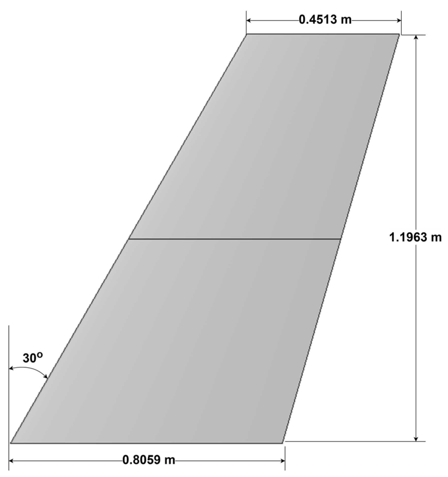
The studies are conducted under sea-level atmospheric properties, with a freestream velocity of $25 \mathrm{m}/\mathrm{s}$. Τwo angles of attack (AoAs) are selected: a moderate 4° and a higher 12°. The latter is commonly more demanding in terms of convergence, requiring more iterations due to the possible flow separation on the suction surface.

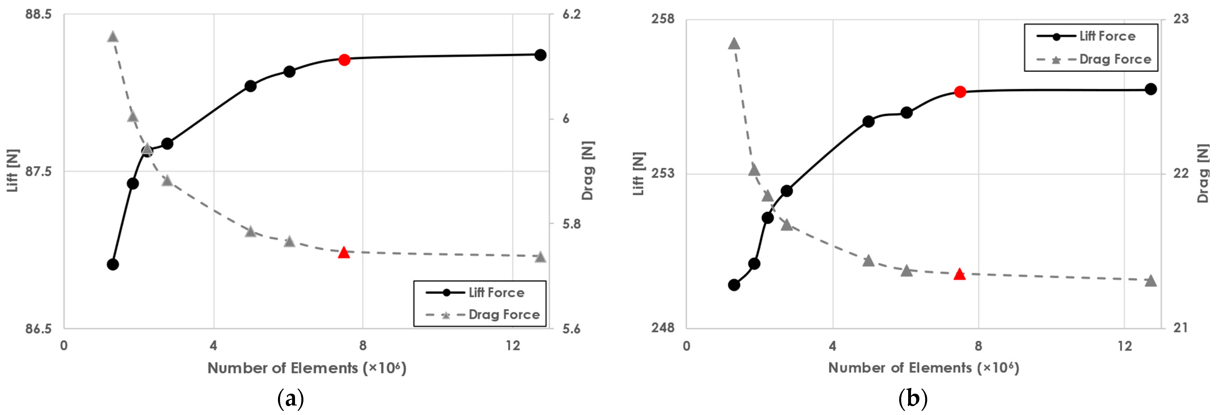
The study is executed by progressively increasing the number of grid elements using a scale factor that affects the hyper-parameters of the meshing algorithm. In Figure 13, the lift and drag forces on the ONERA M6 wing are illustrated for both AoAs.

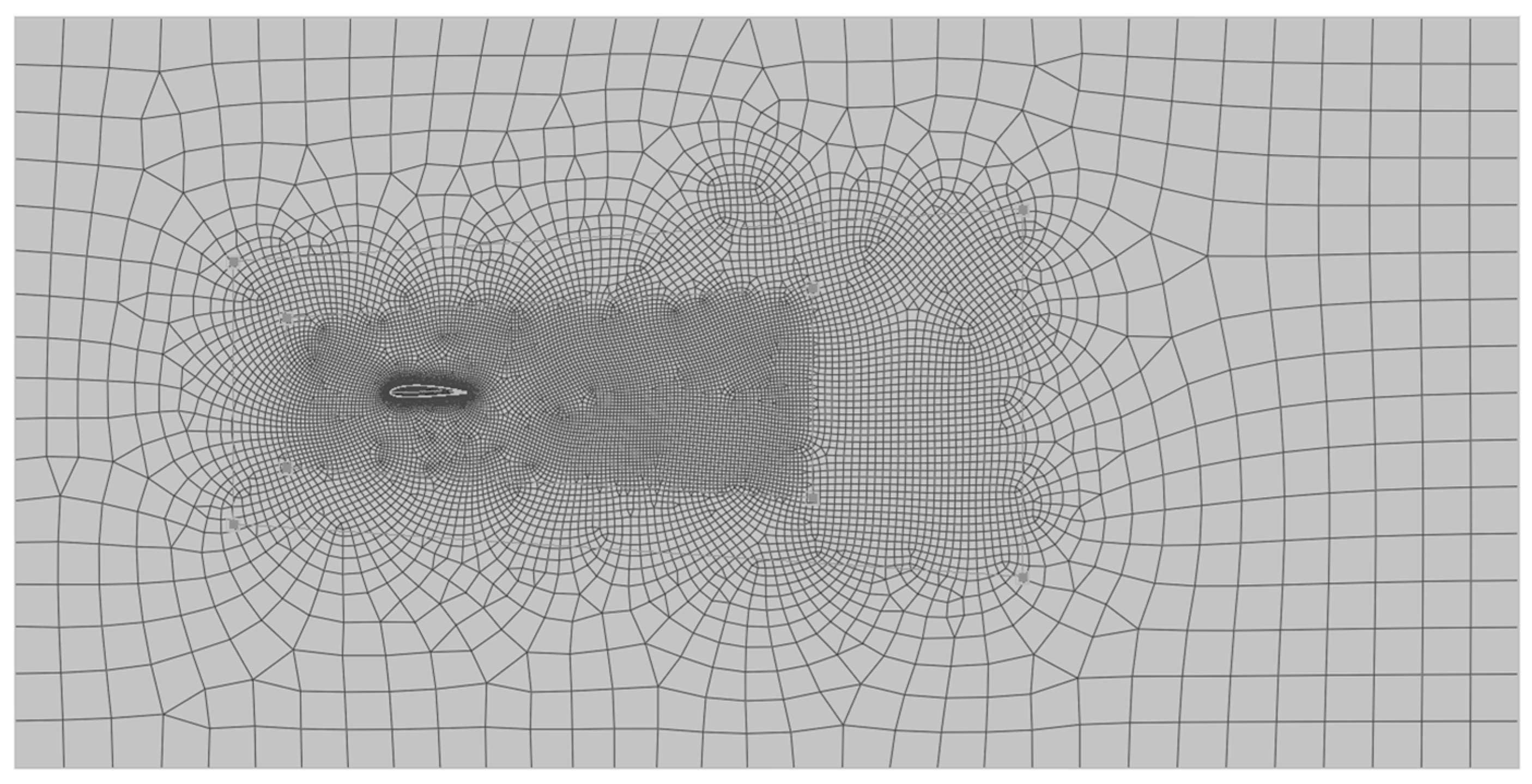
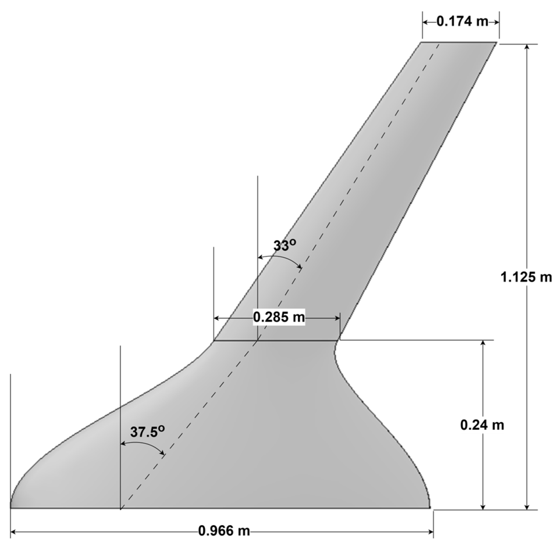
The results highlight that for both cases, the lift and drag forces converge to stable values as the mesh density increases. This also validates the usage of a universal grid per wing and the importance of the BOIs in the proposed framework. Beyond a certain number, which in this case is for approximately 7.5 million grid elements, further refinement provides diminishing returns in accuracy. Thus, the appropriate parameters are being fine-tuned for the meshing module in order to reliably provide computational grids with this refinement. Using these parameters as the baseline, further investigation is being conducted into the determination of the discretization error as per the methodology described in Section 4.1. Three wings are chosen for this phase: the ONERA M6 wing, the RADAERO conventional wing (details are present in Section 6), and a wing belonging to the EURRICA BWB UAV [62]. The planform of the EURRICA wing is illustrated in Figure 14, along with the parametrization in

Table 8. Parametrization of the EURRICA wing.

Parameter	EURRICA *
$c_1$	0.966 m
$c_2$	0.285 m
$c_3$	0.174 m
$b_1$	0.3765 m
$b_2$	1.0433 m
${\Lambda }_1$	37.5°
${\Lambda }_2$	33.0°
$i_1$	-
$i_2$	-
${\gamma }_1$ ${\gamma }_2$	-
	-

* data restrictions apply.

.

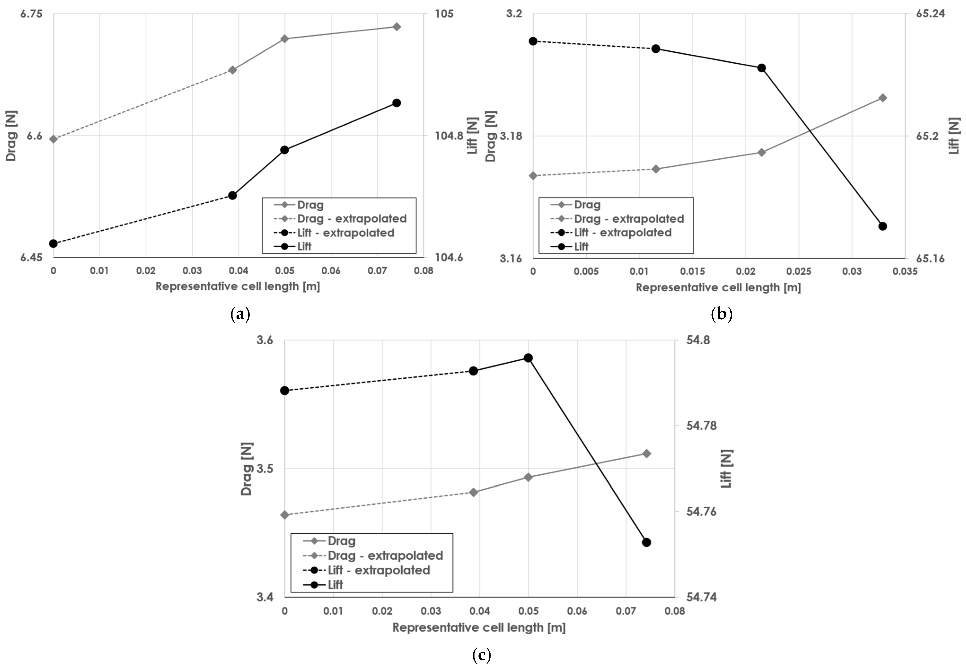
By following this systematic approach, the GCI provides a quantified measure of the discretization error, yielding a transparent assessment of grid-resolution effects. Although GCI is traditionally applied to single-case simulations, this study extends its methodology to the broader design space by evaluating representative samples. The three sampled wings represent the design space of the framework as the most interesting cases. The mean GCI error is used as an aggregated estimate of the discretization error over the design space. In the absence of experimental validation in this study, the GCI remains a credible indicator of numerical errors.

The evaluation metrics for the following grid independence studies are the lift and drag forces. As illustrated in Figure 15, for each case, the least refined computational grid is the one generated using the hyper-parameters selected from the previous grid dependency study. Then, following the GCI approach, systematically more refined grids are created. The final errors calculated are shown in

Table 9. Grid discretization errors.

	Drag			Lift
Platform	$\mathrm{Relative} \mathrm{Error} {\left({\mathit{\epsilon }}_{\mathbf{31}}\right)}_{\mathit{D}\mathit{r}\mathit{a}\mathit{g}}$	$\mathrm{Extrapolated} \mathrm{Relative} \mathrm{Error} {\left({\mathit{\epsilon }}_{\mathbf{3}\mathbf{,}\mathit{e}\mathit{x}\mathit{t}}\right)}_{\mathit{D}\mathit{r}\mathit{a}\mathit{g}}$	Drag GCI31	$\mathrm{Relative} \mathrm{Error} {\left({\mathit{\epsilon }}_{\mathbf{31}}\right)}_{\mathit{L}\mathit{i}\mathit{f}\mathit{t}}$	$\mathrm{Extrapolated} \mathrm{Relative} \mathrm{Error} {\left({\mathit{\epsilon }}_{\mathbf{3}\mathbf{,}\mathit{e}\mathit{x}\mathit{t}}\right)}_{\mathit{L}\mathit{i}\mathit{f}\mathit{t}}$	Lift GCI31
ONERA M6	0.80%	2.10%	1.21%	0.15%	0.22%	0.09%
RADDAERO	0.37%	0.40%	0.06%	0.09%	0.09%	0.02%
EURRICA	0.86%	1.37%	0.40%	0.07%	0.06%	0.03%

.

It is evident that the discretization error for the three cases between the least-fine grid and the extrapolated one, is in the order of 1%. The drag for all cases seems to be more sensitive regarding the grid resolution. This error can be reported as a safe estimate for the grid of this framework.

5.2. Solver Compared with Expert-Grade Results

To evaluate the efficiency and accuracy of the proposed framework, a comparison was conducted against a manually prepared simulation, performed by an experienced CFD mechanical engineer. To ensure consistent and comparable results, the ONERA M6 wing geometry (Figure 12, Table 7) generated by the framework was also provided to the expert. The engineer manually meshed the geometry while preserving the features of the wing. The simulation parameters, including models, solution schemes, and boundary conditions, are appropriately configured to match the setup performed automatically by the framework, as detailed in Algorithm for Convergence Detection section. The validation focuses on key aerodynamic quantities, including the lift coefficient $C_L$, drag coefficient $C_D$, and residual convergence trends. The framework is assessed for its ability to replicate these results while reducing the time and effort required for pre-processing and simulation setup.

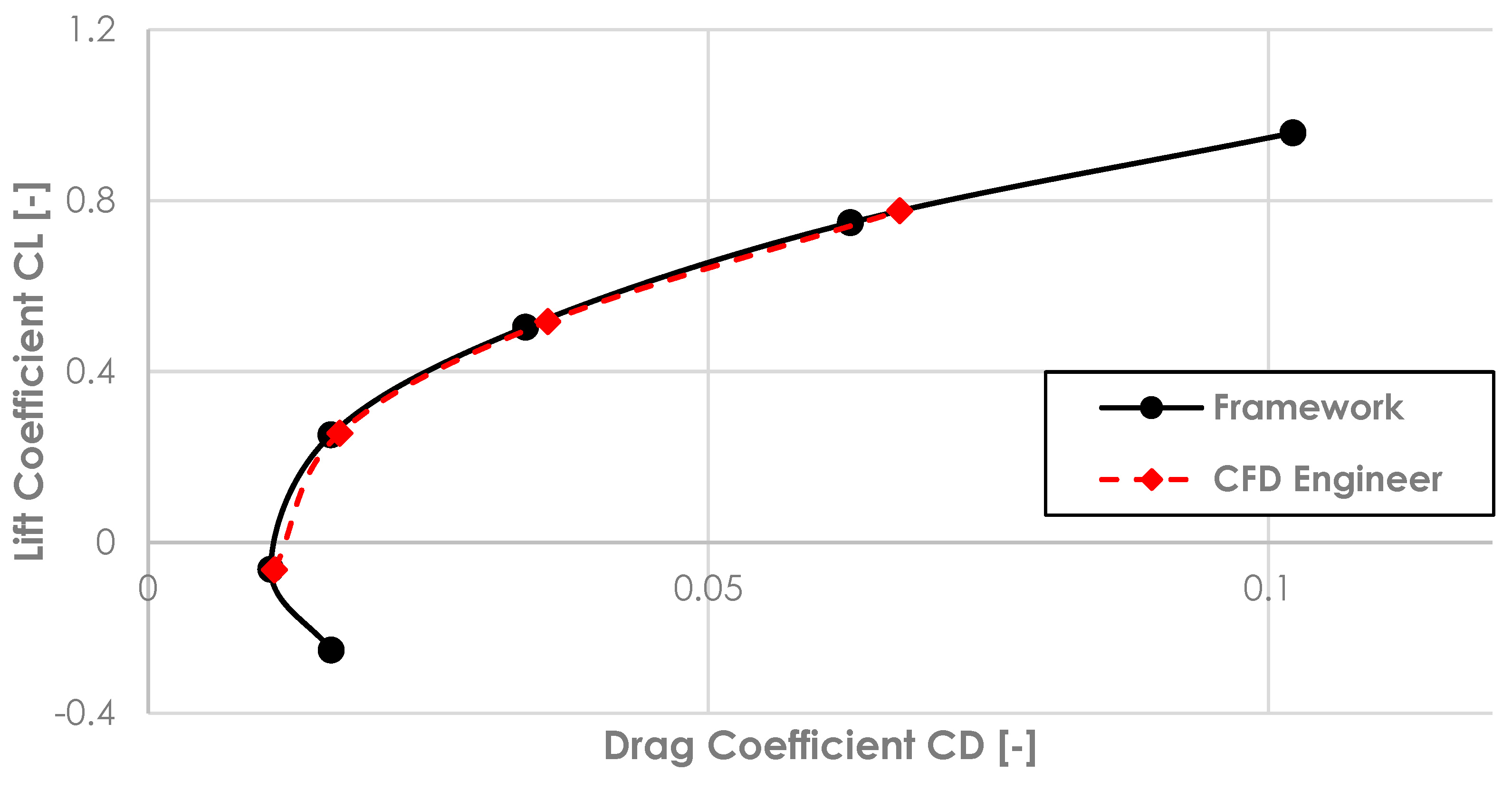
The automated framework demonstrates high reliability, with the drag polar predictions deviating by less than 3% from the manually obtained results. This agreement highlights the framework’s capability to deliver high-level accuracy for subsonic aerodynamic evaluations. As illustrated in Figure 16, the framework successfully captured the lift and drag characteristics across the drag polar of the ONERA M6 wing.

One of the key strengths of the framework lies in its ability to significantly reduce the time required for geometry pre-processing, meshing, and simulation setup. The CFD engineer took approximately 40 min to manually generate the mesh and configure the solver for the ONERA M6 case. In contrast, the automated framework completed these tasks in under 5 min, achieving an 88% reduction in lead time. In this lead time, only the mesh generation and the solution setup are taken into consideration, since the solution execution time is the same for both cases (given that the grid resolution is similar).

5.3. Large Scale Deployment

To evaluate the scalability and robustness of the proposed framework, 1165 wing geometries are sampled from the design space outlined in Section 2. The sampling process employs a Latin Hypercube Sampling (LHS) technique to ensure a uniform distribution of design variables across the multidimensional design space [67]. These sampled wings represent a diverse range of conventional and unconventional configurations, including both conventional wings and more complex blended geometries typically found in tailless, flying wing, or BWB UAVs. 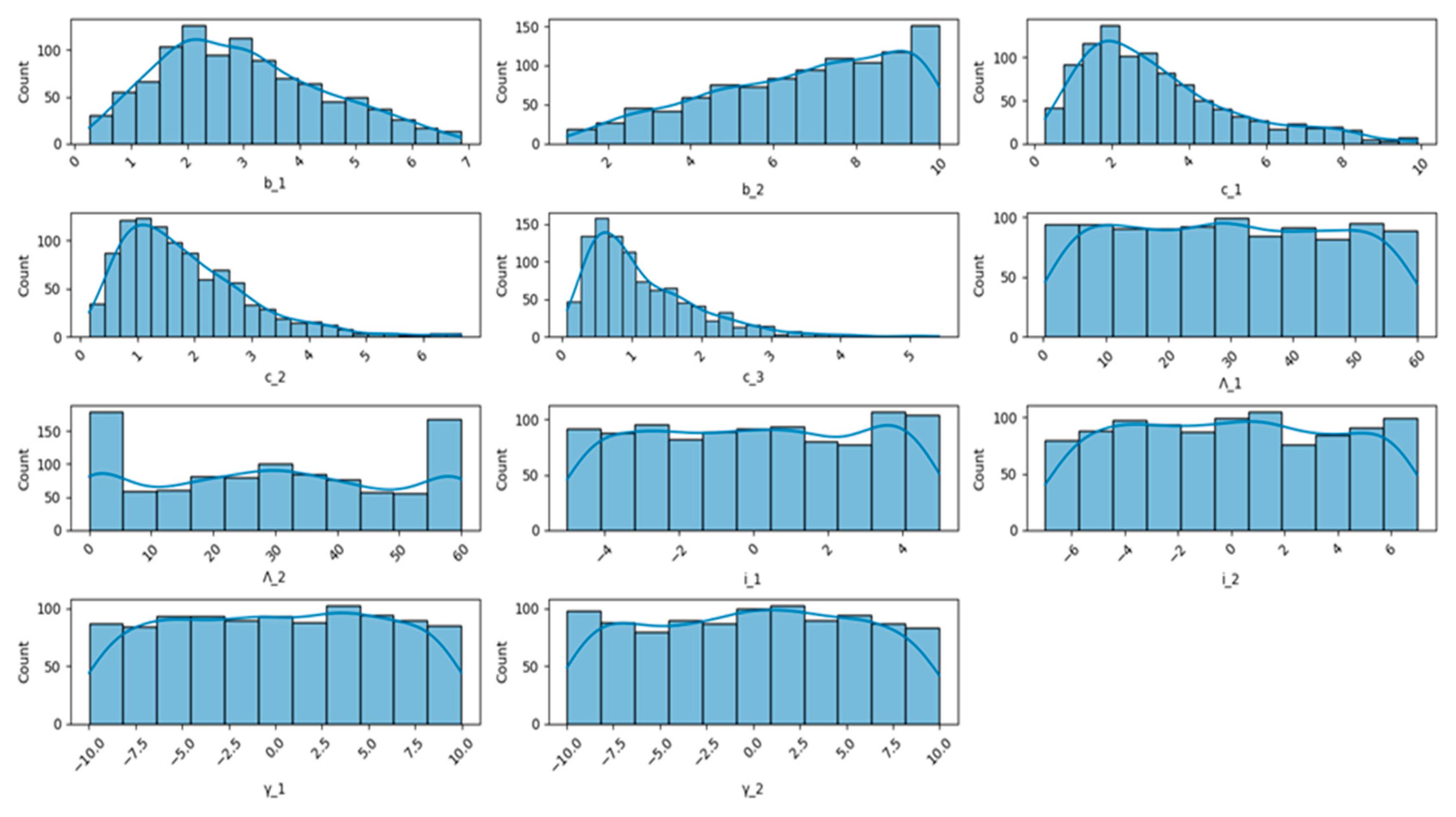Figure 17 provides a visual depiction of the distributions for the high-level planform parameters, illustrating the diversity and coverage achieved in the sampling process.

For each wing configuration, the corresponding flow velocity is sampled according to the methodology described in Section 2. The angle of attack range spans from $-4^{\mathrm{o}}$ to $+{16}^{\mathrm{o}}$, with an additional $4^{\mathrm{o}}$ added in cases where stall has not yet occurred. This approach ensures a comprehensive aerodynamic characterization for each wing. The final dataset comprises 12,858 computational analyses, with an average of 11 simulation runs per configuration. This extensive dataset provides a robust foundation for evaluating the framework’s performance in terms of computational time, robustness, and mesh quality. From the total number of analyses, 96.75% were successfully completed, while the remaining 3.25% encountered issues related to mesh resolution (e.g., $y^{+}$ values) or convergence failure across the majority of runs. Such outcomes offer valuable insights into areas requiring improvement in mesh generation and solver setup for specific configurations.

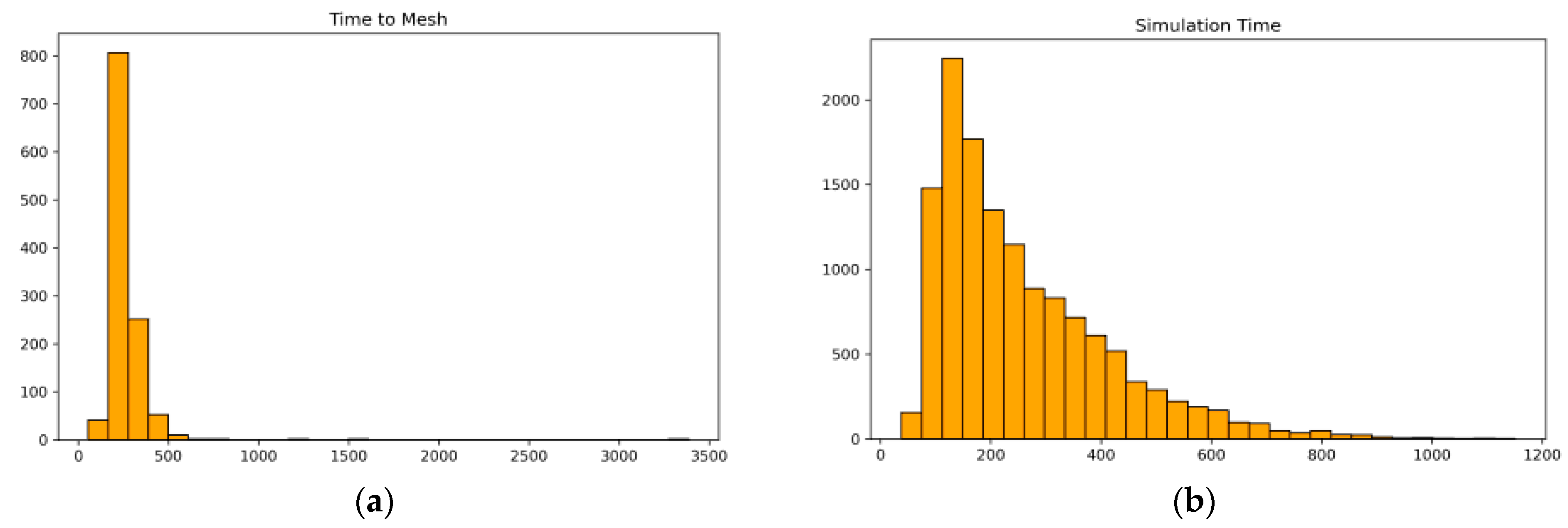
Table 10. Summary statistics of required execution time for 1165 wings (rounded).

Type of Value	Mesh Generation [s]	Writing Mesh to Disk [s]	Loading Mesh in FLUENT [s]	Initializing Solution in FLUENT [s]	Analysis Execution in FLUENT [s]
Minimum Value	54	0.5	1	8	38
Maximum Value	3385	89	115	56	1150
Mean Value	255	36	50	19	259
Median Value	232	33	45	17	212

summarizes execution time statistics across the framework’s main phases, excluding geometry generation, which is negligible in comparison to other modules. From these data, it can be concluded that the median execution time for the pipeline from mesh generation to solution execution is approximately 539 s (9 min), with a standard deviation of 150 s. These results emphasize the framework’s capability to deliver high-fidelity aerodynamic results within a short timeframe, significantly enhancing the efficiency of the design process.

Figure 18 depicts the distribution of the two most time-consuming phases—mesh generation and simulation execution. The distribution plots reveal that mesh generation exhibits less variability compared to simulation execution, which is influenced by the complexity of each configuration.

While as described, $y^{+}$ is not an absolute measure of grid fidelity, it serves as a practical first step in assessing the quality of boundary layer resolution. In contrast, metrics such as the number of prism layers within the boundary layer provide a more comprehensive but inherently complex three-dimensional evaluation, which should be examined as a secondary step by the designer at critical spanwise locations on the wing surface. Equation (13) shows the criteria used to define a high-quality mesh.

$${y_{avg}^{+}}_{@wing\_surface}<1 and {y_{max}^{+}}_{@wing\_surface}<2$$

(13)

Among the 12,858 cases, 93.2% met these quality constraints, indicating a robust and consistent mesh generation process. Outliers, representing 0.5% of cases with abnormal $y^{+}$ values exceeding two orders of magnitude above the quality threshold, are excluded from the analysis.

Table 11. Summary statistics of the results for grid resolution.

Type of Value	${\mathit{y}}_{\mathit{a}\mathit{v}\mathit{e}\mathit{r}\mathit{a}\mathit{g}\mathit{e}}^{+}$	${\mathit{y}}_{\mathit{m}\mathit{a}\mathit{x}\mathit{i}\mathit{m}\mathit{u}\mathit{m}}^{+}$
Minimum	0.32	0.79
Maximum	9.18	29.53
Mean	0.48	1.55
Median	0.46	1.40

provides summary statistics for the $y^{+}$ values of the valid cases.

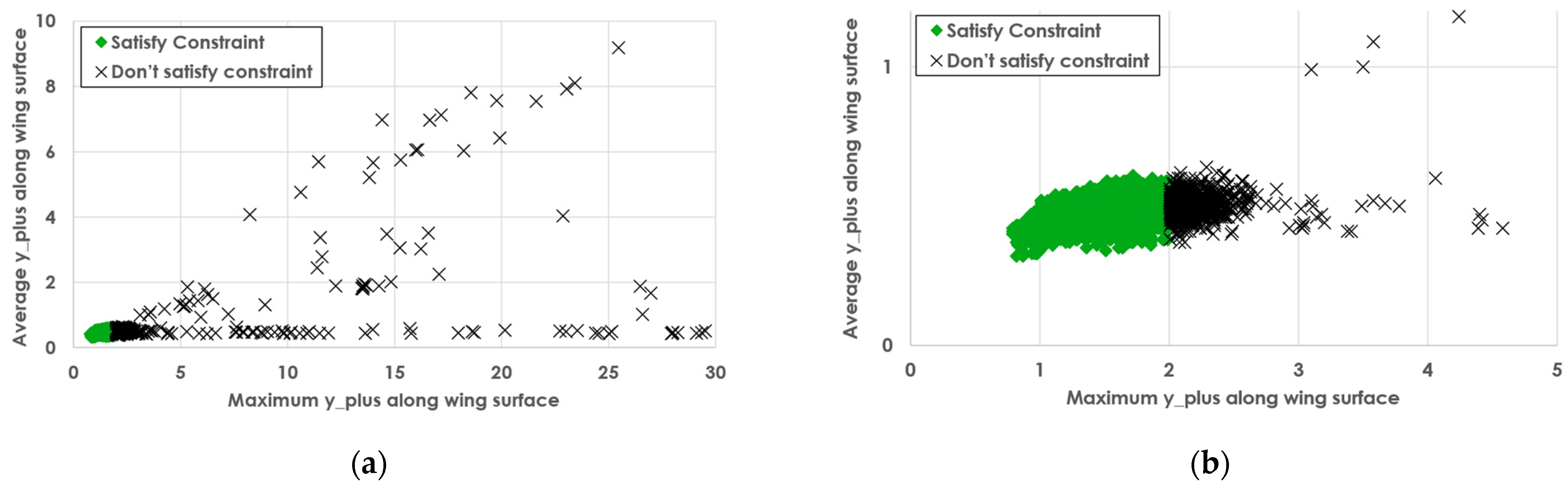
To further analyze the distribution of $y^{+}$ values, Figure 19 provides scatter plots of the average and maximum $y^{+}$ values for all cases. Figure 19a presents the full dataset, excluding the extreme outliers, and highlights the strong clustering of cases that meet the quality criteria, shown by the green diamond points. The presence of a small subset of extreme values, where $y_{max}^{+}$exceeds 10, indicates specific challenges in grid resolution for certain geometries or flow conditions. These cases, although rare, suggest areas for localized adjustments to boundary layer refinement settings.

Figure 19b focuses on cases that satisfy or marginally exceed the quality thresholds, offering a clearer view of the robust performance achieved by the framework. The tightly clustered data points illustrate the consistency of the automated meshing process, particularly for the majority of sampled wings. Overall, these visualizations confirm that the framework maintains a high degree of mesh quality across a diverse range of wing configurations, with only minor deviations requiring further attention.

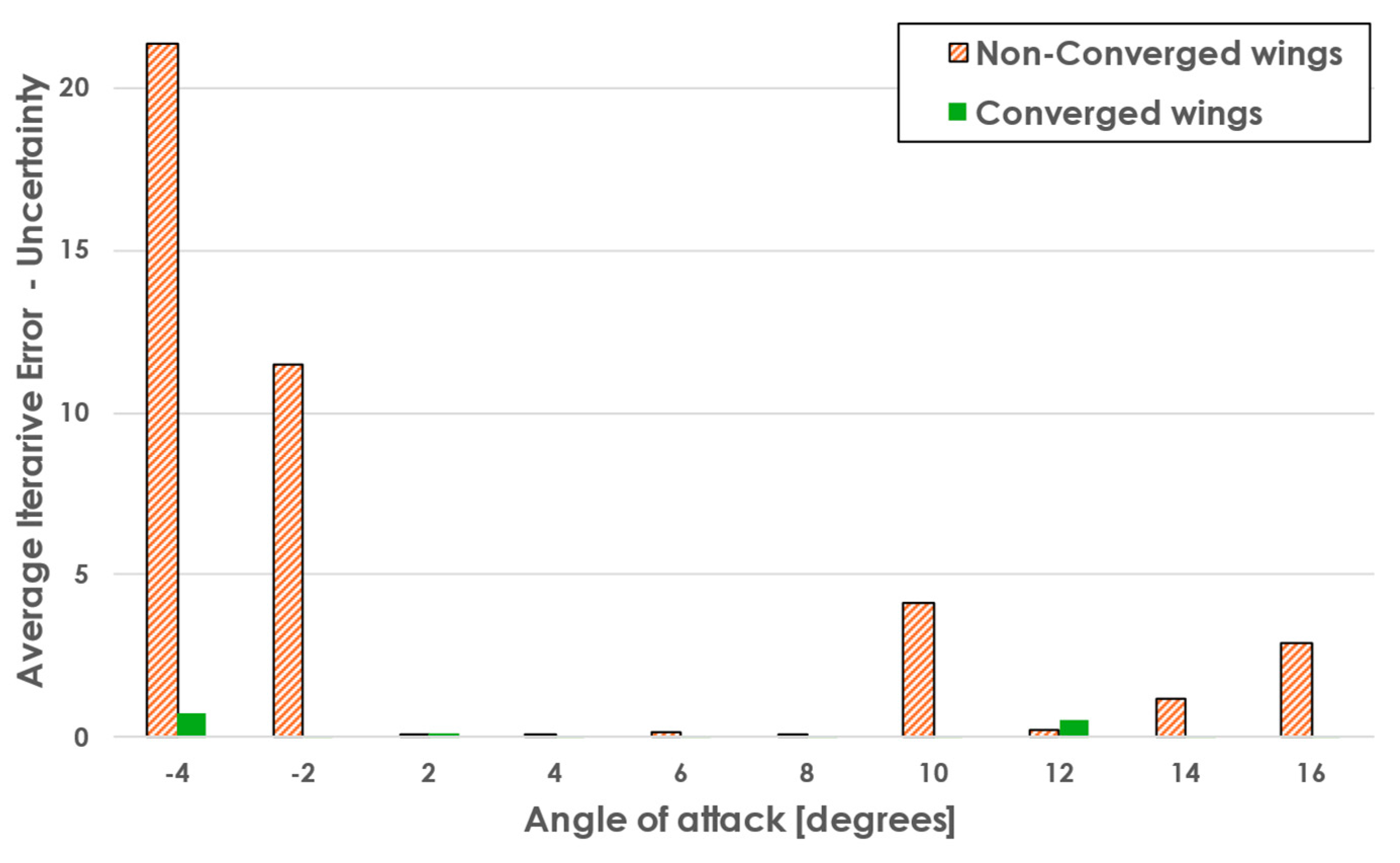
Regarding the iterative error, the same batch of wings is used to investigate the total uncertainty from either non-converged or prematurely converged cases. Solutions are either converged fully or stopped at 2000 iterations (maximum iterations) to assess the impact of incomplete convergence.

Figure 20 illustrates the average iterative error (for both forces in X and Z axis) for converged and non-converged wings across the sampled angles of attack. Non-converged wings exhibit significantly higher iterative errors, particularly at low angles of attack, where the error reaches its peak. In contrast, converged wings demonstrate negligible iterative errors across the entire range, underscoring the importance of convergence in achieving reliable results. This comparison emphasizes the role of iterative errors as a diagnostic tool for assessing the solution quality and the reliability of early terminated simulations.

6. Optimization Case Study

To demonstrate the power of the automated CFD framework, one aerodynamic shape optimization case study is conducted. This includes a conventional UAV wing with the goal of showcasing the adaptability and robustness of the algorithm. The objective of optimization is to maximize the lift-to-drag ($L/D)$ while also satisfying the sensitive stability constraints. All the design variables described in Section 2 are selected, except for the dihedral angle, since it plays a minor role in the aerodynamic performance and the longitudinal stability of the UAV [6,7].

Bayesian Optimization (BO) was chosen for these cases, as it is a method well-suited for high-cost optimization problems [68]. BO utilizes a surrogate model, typically a Gaussian Process (GP), to map the aerodynamic behavior to inputs (i.e., the design variables). The Expected Improvement (EI) criterion drives the algorithm in balancing exploration (unseen design areas) and exploitation (refining promising regions), enabling efficient exploration of high-dimensional design spaces while minimizing the number of analyses required. Classic BO does not offer a straightforward way of incorporating constraints into the optimization formulation. To tackle this, Ref. [69] introduces Constrained Bayesian Optimization (cBO), which incorporates inequality constraints by placing Gaussian Process priors on both the objective and constraint functions. This approach allows for the optimization of an expensive objective function while simultaneously considering feasibility constraints. For the CFD analyses, the AUTh HPC infrastructure was utilized, using the specifications described in Table 6.

Conventional UAV Wing—RADAERO

The RADAERO platform (Figure 21), a conventional fixed-wing UAV with an inverted V-tail configuration, is selected as the reference configuration. The RADAERO platform is a platform that has been 100% designed and built by the Laboratory of Fluid Mechanics and Turbomachinery [70] and has successfully completed several hours of flight testing.

The initial design variables for this case are given in

Table 12. RADAERO wing planform design space.

Design Variable	Baseline *	Lower Bound	Upper Bound
$c_1$	-	0.10–0.50 m
$c_2$	-
$c_3$	-
$b_1$	0.24 m	0.19 m	0.29 m
$b_2$	1.125 m	0.9 m	1.35 m
${\Lambda }_1$	0°	0°	20°
${\Lambda }_2$	0°	0°	20°
$i_1$	-	−2.0–0.0
$i_2$	-

* Data restrictions apply.

. The wing’s airfoil—NACA 2414—and dihedral angle are kept constant along the wing sections. The upper and lower bound of the design variables are constrained to a $\pm 20\%$ from the baseline configuration, ensuring a resemblance to the already designed aircraft. This minimizes the impact of the new wing on the overall performance of the UAV. Flight conditions are fixed at a cruising speed of 25 m/s at sea level, with a reference Reynolds number of 200.000 and an angle of attack of $4^{\mathrm{o}}$. Since RADAERO already features a horizontal and vertical stabilizer, and in a hypothetical scenario of later-stage optimization it imposes a stability constraint on the wing, in order to ensure that the tail remains the same.

The optimization problem formulation is displayed in Equation (14).

$$\begin{gathered} maximize{\displaystyle \frac{L}{D}} \\ \mathrm{subject} \mathrm{to} \left\{\begin{array}{c}{C}_L\ge 0.414\\ 0\le \left|{C_M}_{{\displaystyle \frac{c}{4}}}\right|\le \left|-0.0781\right| \end{array}\right. \end{gathered}$$

(14)

An initial DoE stage (Exploration) is performed, so as to explore the design space. In this phase, using LHS, random configurations are analyzed, thus providing information to the GPs, mapping the inputs to the outputs, and constructing the foundation of feasible and infeasible regions. According to [71,72], the majority of the computational budget should be distributed to the exploitation stage i.e., the infill stage. Guided by the EI acquisition function, the optimizer specifically selects points in the design space that offer a high probability of improving the current best score of the quantity of interest. A total of 30 wing designs are evaluated with a ratio of exploration-to-exploitation equal to 1:2. As illustrated in Figure 22, circles denote valid solutions that satisfy constraints, while crosses represent invalid solutions.

The framework successfully identified a final optimal wing design with an 8% increase in $L/D$, a 2% improvement in $C_L$, and a modest reduction in $C_{M_{c/4}}$, aligning with the constraint (

Table 13. Initial and optimized aerodynamic performance of RADAERO wing.

Variable	Initial Value	After Optimization	Change	${\mathit{y}}_{\mathit{a}\mathit{v}\mathit{g}}^{+}\mathit{o}\mathit{p}\mathit{t}.$	${\mathit{y}}_{\mathit{m}\mathit{a}\mathit{x}}^{+}\mathit{o}\mathit{p}\mathit{t}.$	$\mathit{I}\mathit{t}\mathit{e}\mathit{r}.\mathit{E}\mathit{r}\mathit{r}\mathit{o}\mathit{r}$
$L/D$	19.96	21.52	8%	0.42	1.09	6.85 × 10−4
$C_L$	0.4143	0.4225	2%
$C_M$	−0.0781	−0.076	−2.7%

). On the optimized wing, the average $y^{+}$ value along the wing was kept below 1. This highlights the framework’s effectiveness in navigating a constrained design space, as evidenced by the progressive improvements across iterations and the ability to maintain stability and aerodynamic performance, while also providing reliable and fully automated CFD results.

The optimized wing planform is compared to the baseline in Figure 23. It is evident that the span of the wing increased leading along with its aspect ratio, which has an explicit effect on the reduction in induced drag [7].

7. Conclusions

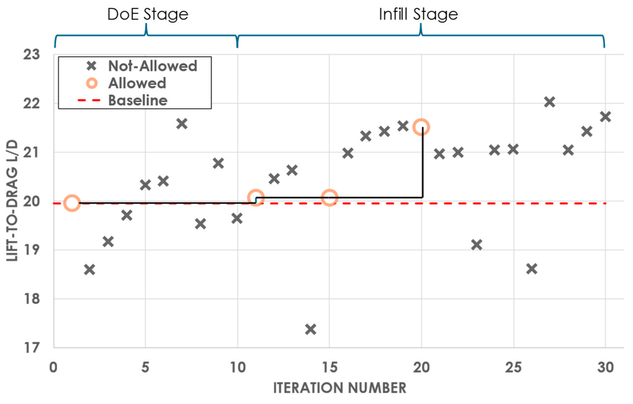
This study presents the development and validation of an automated CFD pre-processing framework designed to streamline high-fidelity aerodynamic simulations tailored for fixed-wing UAV applications. By integrating the geometric modeling, mesh generation, and simulation setup into a cohesive workflow, this framework significantly reduces manual effort and computational inefficiencies. By leveraging Python APIs and a combination of open-source and commercial tools, tshe framework achieves a fully parameterized and automated pipeline, reducing pre-processing times to mere minutes and making it suitable for rapid iterations in design workflows. Moreover, a methodology for estimating the reliability of the framework’s results is proposed, incorporating considerations for discretization error, potential early solution termination, non-dimensional $y^{+}$ values on the wing’s surface, and grid resolution within the boundary layer.

Adhering to best practices and guidelines established by CFD experts and practitioners, the framework demonstrated high accuracy compared to expert-generated results, as well as high consistency across a large number of sampled wings. Additionally, various grid independence studies have been performed, covering a wide range of the design space.

The framework’s integration with high-performance computing (HPC) environments featuring GPU solvers minimizes the labor-intensive work needed to prepare a geometry for CFD simulation. This results in pre-processing durations in the order of 5–7 min and the complete execution of the framework in less than 10–15 min for a single wing at a given angle of attack.

Moreover, the framework is integrated with an off-the-shelf optimizer, functioning as a robust black-box function. Using Bayesian Optimization, the framework identified an optimal wing configuration that achieved an 8% improvement in $L/D$, along with a 2% increase in $C_L$, and a modest reduction in $C_M$. These improvements, while incremental, highlight the framework’s adaptability and demonstrate the advantages of encapsulating all modules within a unified Python pipeline. The framework’s reliable mesh generation ensures seamless execution of cases without computational issues, even under varying conditions.

In summary, the framework represents a significant step forward in streamlining the pre-processing and analysis phases of UAV design. It provides a scalable, efficient, and accurate solution for high-fidelity aerodynamic evaluations, while establishing a robust foundation for future advancements in optimization.

Future work could address the following areas to enhance the framework’s capabilities and expand its scope of use. The framework can be extended to accommodate more complex non-planar features, such as wings with winglets, fins, fences, and tail configurations. Incorporating these components can potentially enable the analysis of complete fixed-wing UAV and aircraft configurations. Moreover, the framework provides a great opportunity to generate large-scale datasets suitable for machine learning applications of aerodynamic shape optimization for UAVs.