
Color Standardization of Chemical Solution Images Using Template-Based Histogram Matching in Deep Learning Regression


Abstract
1. Introduction
2. Related Works
2.1. Color Standardization
2.2. Vitamin C Determination
2.3. Multivariate Regression Algorithms
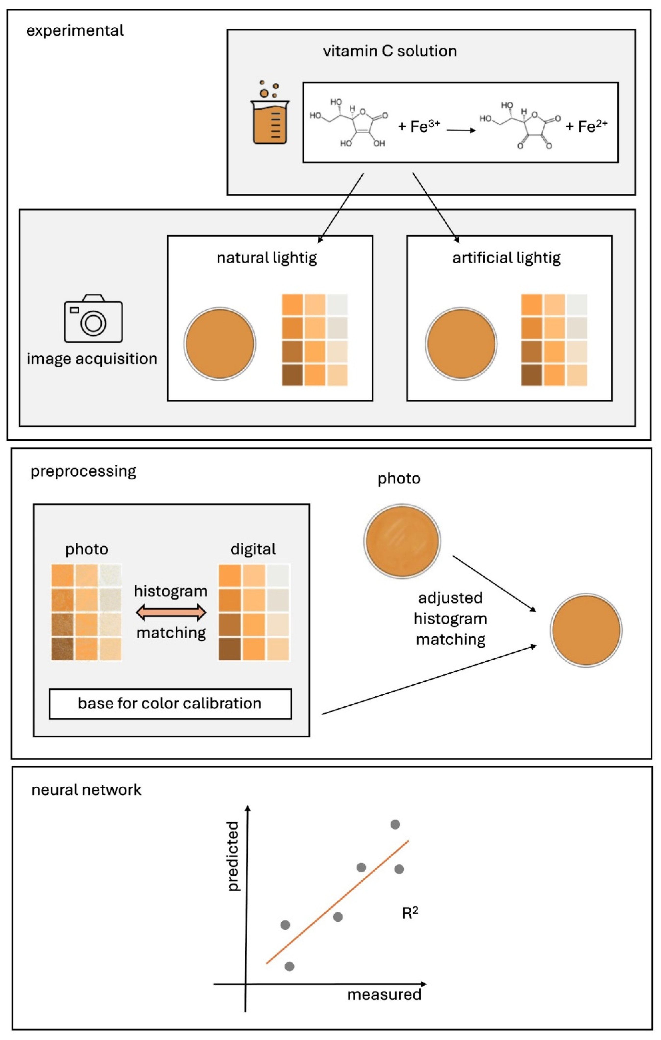
3. Proposed Method
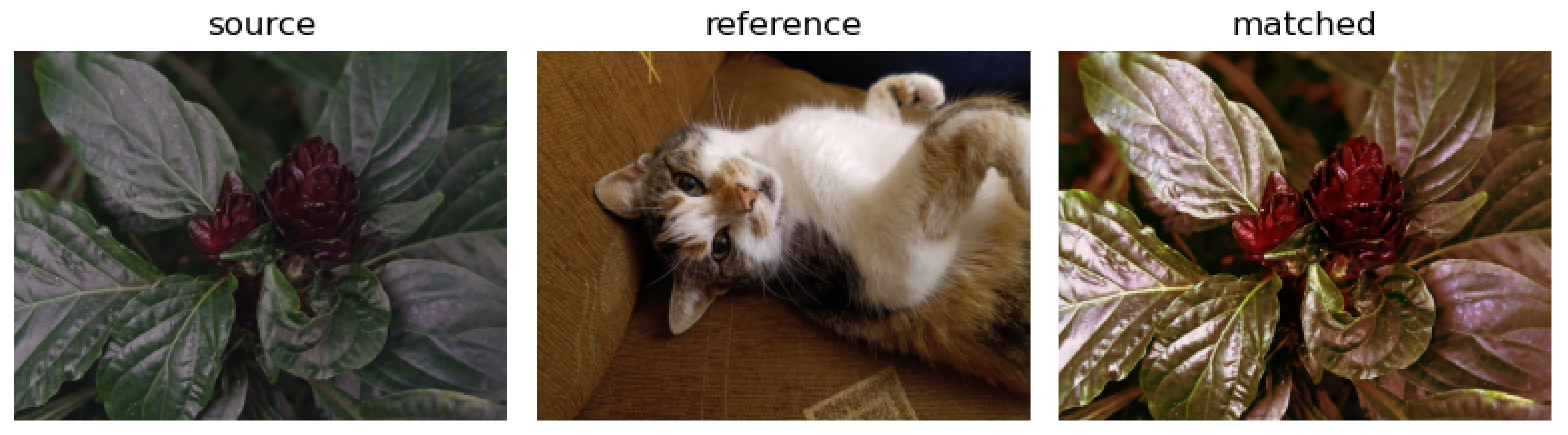
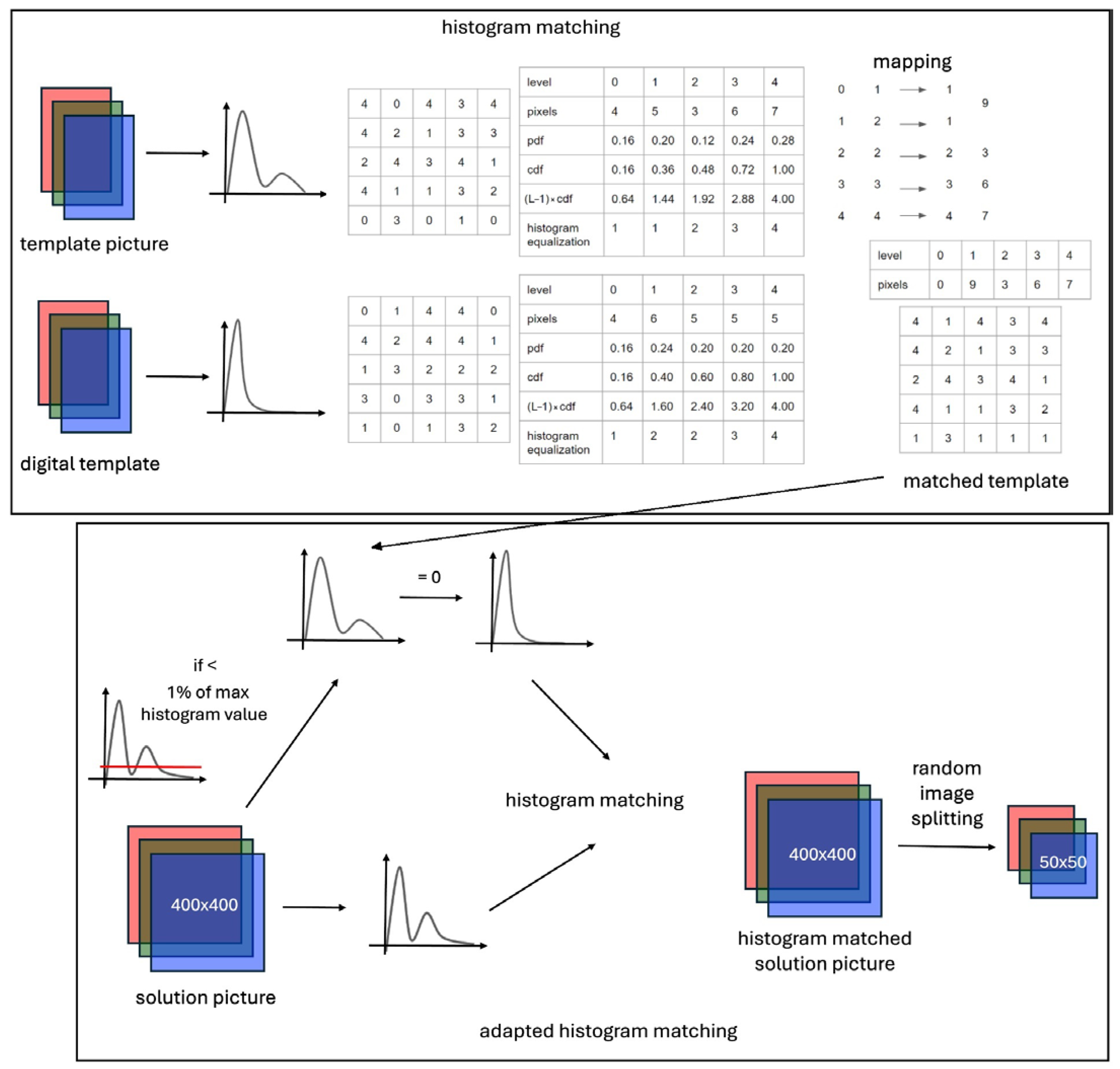
3.1. Color Matching Algorithm
3.2. Software
4. Results and Discussion
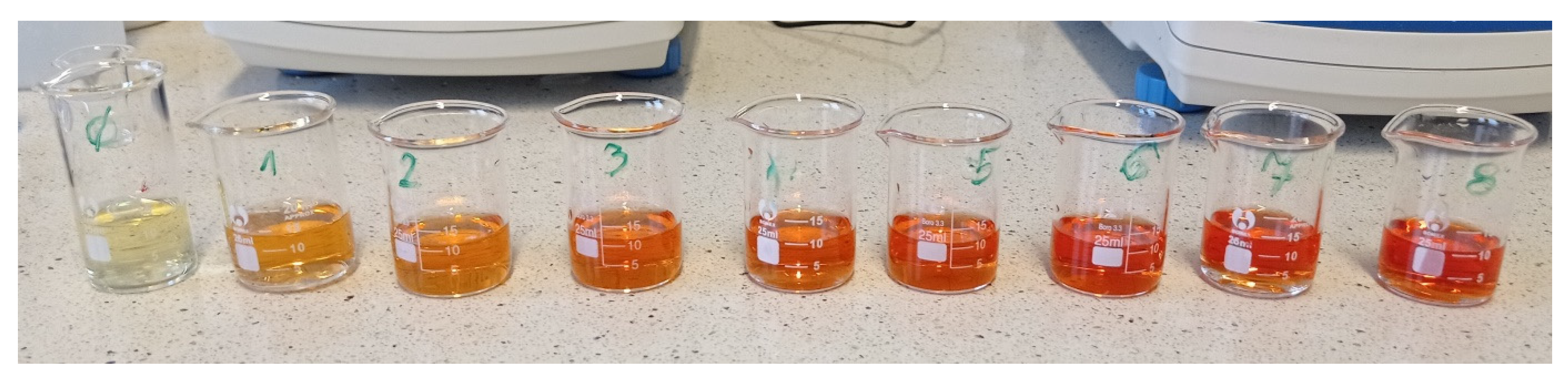
4.1. Reagents, Laboratory Equipment and Measurement Procedure
4.2. Preparation of a Color Template and Picture Acquisition
- training set: 60,416 images
- validation set: 20,480 images
- test set: 20,480 images.
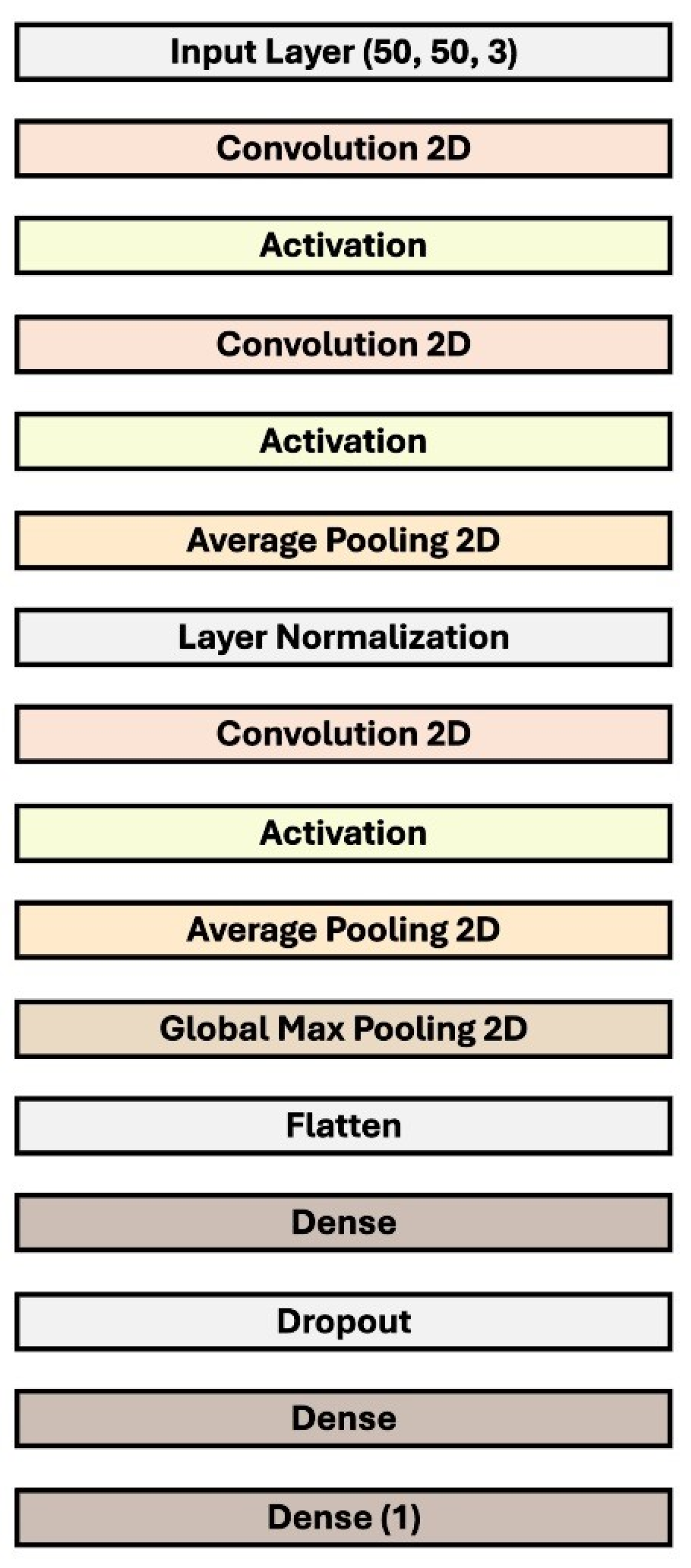
4.3. Network Architecture
4.4. Ablation Study
5. Conclusions
Author Contributions
Funding
Data Availability Statement
Acknowledgments
Conflicts of Interest
References
- Fairchild, M.D. Color Appearance Models, 3rd ed.; John Wiley & Sons, Ltd.: Hoboken, NJ, USA, 2013; ISBN 9781119967033. [Google Scholar]
- Minz, P.S.; Saini, C.S. Evaluation of RGB Cube Calibration Framework and Effect of Calibration Charts on Color Measurement of Mozzarella Cheese. J. Food Meas. Charact. 2019, 13, 1537–1546. [Google Scholar] [CrossRef]
- Ernst, A.; Papst, A.; Ruf, T.; Garbas, J.U. Check My Chart: A Robust Color Chart Tracker for Colorimetric Camera Calibration. In Proceedings of the 6th International Conference on Computer Vision/Computer Graphics Collaboration Techniques and Applications, MIRAGE’13, Berlin, Germany, 6–7 June 2013. [Google Scholar]
- McCamy, C.S.; Marcus, H.; Davidson, J.G. Color-Rendition Chart. J. Appl. Photogr. Eng. 1976, 2, 95–99. [Google Scholar]
- Sunoj, S.; Igathinathane, C.; Saliendra, N.; Hendrickson, J.; Archer, D. Color Calibration of Digital Images for Agriculture and Other Applications. ISPRS J. Photogramm. Remote Sens. 2018, 146, 221–234. [Google Scholar] [CrossRef]
- Kim, M.; Kim, B.; Park, B.; Lee, M.; Won, Y.; Kim, C.Y.; Lee, S. A Digital Shade-Matching Device for Dental Color Determination Using the Support Vector Machine Algorithm. Sensors 2018, 18, 3051. [Google Scholar] [CrossRef]
- Karaimer, H.C.; Brown, M.S. Improving Color Reproduction Accuracy on Cameras. In Proceedings of the IEEE Computer Society Conference on Computer Vision and Pattern Recognition, Salt Lake, UT, USA, 18–23 June 2018; pp. 6440–6449. [Google Scholar]
- Roy, S.; kumar Jain, A.; Lal, S.; Kini, J. A Study about Color Normalization Methods for Histopathology Images. Micron 2018, 114, 42–61. [Google Scholar] [CrossRef]
- Zhao, Y.; Ferguson, S.; Zhou, H.; Elliott, C.; Rafferty, K. Color Alignment for Relative Color Constancy via Non-Standard References. IEEE Trans. Image Process. 2022, 31, 6591–6604. [Google Scholar] [CrossRef]
- Rashid, F.; Jamayet, N.B.; Farook, T.H.; AL-Rawas, M.; Barman, A.; Johari, Y.; Noorani, T.Y.; Abdullah, J.Y.; Eusufzai, S.Z.; Alam, M.K. Color Variations during Digital Imaging of Facial Prostheses Subjected to Unfiltered Ambient Light and Image Calibration Techniques within Dental Clinics: An In Vitro Analysis. PLoS ONE 2022, 17, e0273029. [Google Scholar] [CrossRef]
- Barbero-Álvarez, M.A.; Rodrigo, J.A.; Menéndez, J.M. Minimum Error Adaptive RGB Calibration in a Context of Colorimetric Uncertainty for Cultural Heritage Preservation. Comput. Vis. Image Underst. 2023, 237, 103835. [Google Scholar] [CrossRef]
- Noor Azhar, M.; Bustam, A.; Naseem, F.S.; Shuin, S.S.; Md Yusuf, M.H.; Hishamudin, N.U.; Poh, K. Improving the Reliability of Smartphone-Based Urine Colorimetry Using a Colour Card Calibration Method. Digit. Health 2023, 9, 20552076231154684. [Google Scholar] [CrossRef]
- Zhang, G.; Song, S.; Panescu, J.; Shapiro, N.; Dannemiller, K.C.; Qin, R. A Novel Systems Solution for Accurate Colorimetric Measurement through Smartphone-Based Augmented Reality. PLoS ONE 2023, 18, e0287099. [Google Scholar] [CrossRef]
- Chairat, S.; Chaichulee, S.; Dissaneewate, T.; Wangkulangkul, P.; Kongpanichakul, L. AI-Assisted Assessment of Wound Tissue with Automatic Color and Measurement Calibration on Images Taken with a Smartphone. Healthcare 2023, 11, 273. [Google Scholar] [CrossRef]
- Suominen, J.; Egiazarian, K. Camera Color Correction Using Splines. In Proceedings of the IS&T International Symposium on Electronic Imaging, Burlingame, CA, USA, 21–25 January 2024; pp. 165-1–165-6. [Google Scholar]
- Souissi, M.; Chaouch, S.; Moussa, A. Color Matching of Bicomponent (PET/PTT) Filaments with High Performances Using Genetic Algorithm. Sci. Rep. 2024, 14, 10949. [Google Scholar] [CrossRef]
- Wannasin, D.; Grossmann, L.; McClements, D.J. Optimizing the Appearance of Plant-Based Foods Using Natural Pigments and Color Matching Theory. Food Biophys. 2024, 19, 120–130. [Google Scholar] [CrossRef]
- Wu, Y. Reference Image Aided Color Matching Design Based on Interactive Genetic Algorithm. J. Electr. Syst. 2024, 20, 400–410. [Google Scholar] [CrossRef]
- Food and Agriculture Organization; World Health Organization. Vitamin and Mineral Requirements in Human Nutrition, 2nd ed.; FAO/WHO: Geneva, Switzerland, 1998; pp. 1–20. ISBN 9241546123. [Google Scholar]
- Food and Agriculture Organization; World Health Organization. Human Vitamin and Mineral Requirements; FAO/WHO: Geneva, Switzerland, 2001. [Google Scholar]
- Lykkesfeldt, J. On the Effect of Vitamin C Intake on Human Health: How to (Mis)Interprete the Clinical Evidence. Redox Biol. 2020, 34, 101532. [Google Scholar] [CrossRef]
- Dosed, M.; Jirkovsk, E.; Kujovsk, L.; Javorsk, L.; Pourov, J.; Mercolini, L.; Remi, F. Vitamin C—Sources, Physiological Role, Kinetics, Deficiency, Use, Toxicity, and Determination. Nutrients 2021, 615, 1–34. [Google Scholar]
- Suntornsuk, L.; Gritsanapun, W.; Nilkamhank, S.; Paochom, A. Quantitation of Vitamin C Content in Herbal Juice Using Direct Titration. J. Pharm. Biomed. Anal. 2002, 28, 849–855. [Google Scholar] [CrossRef]
- Klimczak, I.; Gliszczyńska-Świgło, A. Comparison of UPLC and HPLC Methods for Determination of Vitamin C. Food Chem. 2015, 175, 100–105. [Google Scholar] [CrossRef]
- Gazdik, Z.; Zitka, O.; Petrlova, J.; Adam, V.; Zehnalek, J.; Horna, A.; Reznicek, V.; Beklova, M.; Kizek, R. Determination of Vitamin C (Ascorbic Acid) Using High Performance Liquid Chromatography Coupled with Electrochemical Detection. Sensors 2008, 8, 7097–7112. [Google Scholar] [CrossRef]
- Bunaciu, A.A.; Bacalum, E.; Aboul-Enein, H.Y.; Udristioiu, G.E.; Fleschin, Ş. FT-IR Spectrophotometric Analysis of Ascorbic Acid and Biotin and Their Pharmaceutical Formulations. Anal. Lett. 2009, 42, 1321–1327. [Google Scholar] [CrossRef]
- Zhu, Q.; Dong, D.; Zheng, X.; Song, H.; Zhao, X.; Chen, H.; Chen, X. Chemiluminescence Determination of Ascorbic Acid Using Graphene Oxide@copper-Based Metal-Organic Frameworks as a Catalyst. RSC Adv. 2016, 6, 25047–25055. [Google Scholar] [CrossRef]
- Berg, R.W. Investigation of L (+)-Ascorbic Acid with Raman Spectroscopy in Visible and UV Light. Appl. Spectrosc. Rev. 2015, 50, 193–239. [Google Scholar] [CrossRef]
- Yang, H.; Irudayaraj, J. Rapid Determination of Vitamin C by NIR, MIR and FT-Raman Techniques. J. Pharm. Pharmacol. 2010, 54, 1247–1255. [Google Scholar] [CrossRef]
- Zykova, E.V.; Sandetskaya, N.G.; Ostrovskii, O.V.; Verovskii, V.E. Methods of Analysis and Process Control Determining Ascorbic Acid in Medicinal Preparations By Capillary Zone Electrophoresis and Micellar. Pharm. Chem. J. 2010, 44, 463–465. [Google Scholar] [CrossRef]
- Dodevska, T.; Hadzhiev, D.; Shterev, I. A Review on Electrochemical Microsensors for Ascorbic Acid Detection: Clinical, Pharmaceutical, and Food Safety Applications. Micromachines 2023, 14, 41. [Google Scholar] [CrossRef]
- Huang, L.; Tian, S.; Zhao, W.; Liu, K.; Guo, J. Electrochemical Vitamin Sensors: A Critical Review. Talanta 2021, 222, 121645. [Google Scholar] [CrossRef]
- Broncová, G.; Prokopec, V.; Shishkanova, T.V. Potentiometric Electronic Tongue for Pharmaceutical Analytics: Determination of Ascorbic Acid Based on Electropolymerized Films. Chemosensors 2021, 9, 110. [Google Scholar] [CrossRef]
- Coutinho, M.S.; Morais, C.L.M.; Neves, A.C.O.; Menezes, F.G.; Lima, K.M.G. Colorimetric Determination of Ascorbic Acid Based on Its Interfering Effect in the Enzymatic Analysis of Glucose: An Approach Using Smartphone Image Analysis. J. Braz. Chem. Soc. 2017, 28, 2500–2505. [Google Scholar] [CrossRef]
- Porto, I.S.A.; Santos Neto, J.H.; dos Santos, L.O.; Gomes, A.A.; Ferreira, S.L.C. Determination of Ascorbic Acid in Natural Fruit Juices Using Digital Image Colorimetry. Microchem. J. 2019, 149, 104031. [Google Scholar] [CrossRef]
- Kong, L.; Gan, Y.; Liang, T.; Zhong, L.; Pan, Y.; Kirsanov, D.; Legin, A.; Wan, H.; Wang, P. A Novel Smartphone-Based CD-Spectrometer for High Sensitive and Cost-Effective Colorimetric Detection of Ascorbic Acid. Anal. Chim. Acta 2020, 1093, 150–159. [Google Scholar] [CrossRef]
- Li, C.; Xu, X.; Wang, F.; Zhao, Y.; Shi, Y.; Zhao, X.; Liu, J. Portable Smartphone Platform Integrated with Paper Strip-Assisted Fluorescence Sensor for Ultrasensitive and Visual Quantitation of Ascorbic Acid. Food Chem. 2023, 402, 134222. [Google Scholar] [CrossRef]
- Zhaoa, W.; Caoa, P.; Zhua, Y.; Liua, S.; Gaob, H.-W.; Huang, C. Rapid Detection of Vitamin C Content in Fruits and Vegetables Using a Digital Camera and Color Reaction. Quim. Nov. 2020, 43, 1421–1430. [Google Scholar] [CrossRef]
- Dumancas, G.G.; Ramasahayam, S.; Bello, G.; Hughes, J.; Kramer, R. Chemometric Regression Techniques as Emerging, Powerful Tools in Genetic Association Studies. TrAC Trends Anal. Chem. 2015, 74, 79–88. [Google Scholar] [CrossRef]
- Wold, S.; Sjöström, M.; Eriksson, L. PLS-Regression: A Basic Tool of Chemometrics. Chemom. Intell. Lab. Syst. 2001, 58, 109–130. [Google Scholar] [CrossRef]
- Li, B.; Morris, J.; Martin, E.B. Model Selection for Partial Least Squares Regression. Chemom. Intell. Lab. Syst. 2002, 64, 79–89. [Google Scholar] [CrossRef]
- Smola, A.J.; Schokopf, B. A Tutorial on Support Vector Regression. Stat. Comput. 2004, 14, 199–222. [Google Scholar] [CrossRef]
- Goodfellow, I.; Bengio, Y.; Courville, A. Deep Learning; MIT Press: Cambridge, MA, USA, 2016; ISBN 9780262035613. [Google Scholar]
- Lathuiliere, S.; Mesejo, P.; Alameda-Pineda, X.; Horaud, R. A Comprehensive Analysis of Deep Regression. IEEE Trans. Pattern Anal. Mach. Intell. 2020, 42, 2065–2081. [Google Scholar] [CrossRef]
- Pascual, L.; Gras, M.; Vidal-Brotóns, D.; Alcañiz, M.; Martínez-Máñez, R.; Ros-Lis, J.V. A Voltammetric E-Tongue Tool for the Emulation of the Sensorial Analysis and the Discrimination of Vegetal Milks. Sens. Actuators B Chem. 2018, 270, 231–238. [Google Scholar] [CrossRef]
- Wójcik, S.; Ciepiela, F.; Jakubowska, M. Computer Vision Analysis of Sample Colors versus Quadruple-Disk Iridium-Platinum Voltammetric e-Tongue for Recognition of Natural Honey Adulteration. Meas. J. Int. Meas. Confed. 2023, 209, 112514. [Google Scholar] [CrossRef]
- Lee, M. Mathematical Analysis and Performance Evaluation of the GELU Activation Function in Deep Learning. J. Math. 2023, 1, 4229924. [Google Scholar] [CrossRef]
- Sikandar, S.; Mahum, R.; Alsalman, A.M. A Novel Hybrid Approach for a Content-Based Image Retrieval Using Feature Fusion. Appl. Sci. 2023, 13, 4581. [Google Scholar] [CrossRef]
- Hasan, M.A.; Haque, F.; Sabuj, S.R.; Sarker, H.; Goni, M.O.F.; Rahman, F.; Rashid, M.M. An End-to-End Lightweight Multi-Scale CNN for the Classification of Lung and Colon Cancer with XAI Integration. Technologies 2024, 12, 56. [Google Scholar] [CrossRef]


| Ref. | Year | Problem Solved | Dataset Used | Color Correction Strategy |
|---|---|---|---|---|
| [9] | 2022 | The general concept of relative color constancy (RCC) i.e., the ability to align colors of the same objects between images independent of illumination and camera | Three image datasets collected by multiple cameras under various illumination and exposure conditions (Belfast, Middlebury, Gehler-Shi) | Three steps of color alignment framework: camera response calibration with color patches, response linearization, pixel-wise color intensity, and chromaticity matching |
| [10] | 2022 | Color variations within clinical images of maxillofacial prosthetic silicone specimens (in vitro approach) | Images of the pigmented prosthetic silicone specimens within different ambient lighting conditions | Computerized software-based post-processing white balance calibration (PPWBC) using a gray card and Macbeth color chart |
| [11] | 2023 | Non-invasive cultural heritage conservation in the context of material degradation | Four sets of images in different lighting conditions, acquired with a conventional cellphone camera in sRGB color space | An adaptive transfer function, working with a self-made color calibration chart; neural network-based final tuning of the calibration functions |
| [12] | 2023 | Smartphone-based urine colorimetry | Urine samples from 58 patients photographed in a customized photo box, under five simulated lighting conditions, using five smartphones in RGB color space | Color calibration with SpyderCHEKRTM color chart and the Adobe Photoshop proprietary algorithms to scale the uncorrected RGB values |
| [13] | 2023 | A smartphone-based solution for accurate colorimetric measurements, with an augmented-reality guiding system | Simulated and real images, images of color stripe kits for pH reading | A color correction algorithm with the first-order spatial varying regression model which leverages both the absolute color magnitude and scale; the system includes a color reference board |
| [14] | 2023 | Assessment of the healing process of chronic wounds | Wound tissue images taken at different times, under different lighting conditions, distances, lenses, and smartphone cameras in RGB color space | Images of wound tissue taken with a Macbeth chart of 24 square color patches and four ArUco markers at corners of the chart; transformation matrix calculation using the Moore–Penrose inverse matrix and the target matrix |
| [15] | 2024 | A general purpose algorithm | Photos of nature and city landscapes, vegetation, and human-made objects in RGB color space | A matrix-based transformation using tensor product B-splines with optimization of the smoothing parameter λ and number of spline basis functions |
| [16] | 2024 | Reproduction of reference color of textile clothing by selecting appropriate disperse dyes | Results of colorimetric measurements using a spectrophotometer type Spectraflash 600 Plus (Datacolor International, USA) | A genetic algorithm to optimize the selection and concentration of dyes for exact color matching in bicomponent (PET/PTT) filaments |
| [17] | 2024 | Optimization of the appearances of plant-based foods considering that animal-based products may contain a wide range of different pigments and structural elements that scatter light | L*, a*, b* values of animal-based products and plant-based emulsions produced measured by colorimeter (ColorFlex EZ 45/0-LAV, Hunter Associates Laboratory Inc., Reston, VA, USA) | The color matching model based on Kubelka–Munk theory, used to calculate the spectral reflectance of the mixed emulsions from the spectral reflectance of the individual color-loaded emulsions |
| [18] | 2024 | Color design for fashion—color selection and matching different color combinations | Graphic objects designed in CorelDraw | Color matching based on an interactive genetic algorithm using reference images |
| Layer (Type) | Output Shape | Number of Parameters |
|---|---|---|
| Input layer | (None, 50, 50, 3) | 0 |
| Conv2D | (None, 50, 50,3 2) | 128 |
| Activation | (None, 50, 50, 32) | 0 |
| Conv2D | (None, 50, 50, 64) | 2112 |
| Activation | (None, 50, 50, 64) | 0 |
| AveragePooling2D | (None, 46, 46, 64) | 0 |
| LayerNormalization | (None, 46, 46, 64) | 128 |
| Conv2D | (None, 46, 46, 64) | 4160 |
| Activation | (None, 46, 46, 64) | 0 |
| AveragePooling2D | (None, 44, 44, 64) | 0 |
| GlobalMaxPooling2D | (None, 64) | 0 |
| Flatten | (None, 64) | 0 |
| Dense | (None, 150) | 9750 |
| Dropout | (None, 150) | 0 |
| Dense | (None, 50) | 7550 |
| Dense | (None, 1) | 51 |
| Total params: 23,879 (93.28 KB) Trainable params: 23,879 (93.28 KB) Non-trainable params: 0 (0.00 Byte) | ||
| Parameter | Setting |
|---|---|
| Image size | 50 × 50 × 3 |
| Loss function | MSE + MAE |
| Optimizer | Adam |
| Initial learning rate | 0.001 |
| Metric | RMSE |
| Batch size | 30 |
| Epoch | 20 |
| Shuffle | Every epoch |
| Artificial Lighting, Original | Artificial Lighting, Matched | Natural Lighting, Original | Natural Lighting, Matched | Mixed Lighting, Original | Mixed Lighting, Matched | |
|---|---|---|---|---|---|---|
| Slope | 0.9799 | 0.9961 | 0.9706 | 0.9452 | 0.9784 | 0.9825 |
| Intercept | −0.0036 | −0.2091 | 1.1888 | 0.6051 | 0.5832 | 0.4086 |
| RMSE/µg·mL−1 | 1.5769 | 0.7525 | 2.2900 | 1.9542 | 1.4828 | 1.3510 |
| R2 score | 0.9979 | 0.9999 | 0.9953 | 0.9956 | 0.9966 | 0.9968 |
| Artificial Lighting, Original | Artificial Lighting, Matched | Natural Lighting, Original | Natural Lighting, Matched | Mixed Lighting, Original | Mixed Lighting, Matched | |
|---|---|---|---|---|---|---|
| Slope | 0.9058 | 1.0138 | 0.9538 | 1.0071 | 1.0005 | 1.0112 |
| Intercept | 0.6891 | −0.3598 | −0.8347 | 0.2263 | 0.8747 | 0.0203 |
| RMSE/µg·mL−1 | 5.8415 | 1.7077 | 3.9504 | 2.5151 | 4.3488 | 2.8211 |
| R2 score | 0.9557 | 0.9962 | 0.9798 | 0.9918 | 0.9755 | 0.9897 |
| Change in Architecture | RMSE/µg·mL−1 | R2 Score | Comparison |
|---|---|---|---|
| Batch size = 120 | 2.3535 | 0.9947 | Decrease of R2 score and increase of RMSE in comparison to final model. |
| Image size = 16 | 4.0146 | 0.9825 | Significant decrease of R2 score and increase of RMSE in comparison to final model. Lower decline of initial rate in comparison to final version. |
| Loss function modification | 3.8203 | 0.9856 | Decrease of R2 score and significant increase of RMSE in comparison to final model. Minimized differences between training and validation loss during training. |
| Optimizer = Adagrad | 3.1625 | 0.9877 | Decrease of R2 score and increase of RMSE in comparison to final model. |
| Optimizer = SGD | - | - | There was no change in loss value between the epochs. The model did not learn to predict the concentration of vitamin C solutions. |
| Initial learning rate = 0.01 or 0.0001 | - | - | No significant change in the results was detected. The results achieved did not vary significantly in comparison to final model results. |
Disclaimer/Publisher’s Note: The statements, opinions and data contained in all publications are solely those of the individual author(s) and contributor(s) and not of MDPI and/or the editor(s). MDPI and/or the editor(s) disclaim responsibility for any injury to people or property resulting from any ideas, methods, instructions or products referred to in the content. |
© 2024 by the authors. Licensee MDPI, Basel, Switzerland. This article is an open access article distributed under the terms and conditions of the Creative Commons Attribution (CC BY) license (https://creativecommons.org/licenses/by/4.0/).
Share and Cite
Kwiek, P.; Jakubowska, M. Color Standardization of Chemical Solution Images Using Template-Based Histogram Matching in Deep Learning Regression. Algorithms 2024, 17, 335. https://doi.org/10.3390/a17080335
Kwiek P, Jakubowska M. Color Standardization of Chemical Solution Images Using Template-Based Histogram Matching in Deep Learning Regression. Algorithms. 2024; 17(8):335. https://doi.org/10.3390/a17080335
Chicago/Turabian StyleKwiek, Patrycja, and Małgorzata Jakubowska. 2024. "Color Standardization of Chemical Solution Images Using Template-Based Histogram Matching in Deep Learning Regression" Algorithms 17, no. 8: 335. https://doi.org/10.3390/a17080335
APA StyleKwiek, P., & Jakubowska, M. (2024). Color Standardization of Chemical Solution Images Using Template-Based Histogram Matching in Deep Learning Regression. Algorithms, 17(8), 335. https://doi.org/10.3390/a17080335