Abstract
HER2 overexpression is a prognostic and predictive factor observed in about 15% to 20% of breast cancer cases. The assessment of its expression directly affects the selection of treatment and prognosis. The measurement of HER2 status is performed by an expert pathologist who assigns a score of 0, 1, 2+, or 3+ based on the gene expression. There is a high probability of interobserver variability in this evaluation, especially when it comes to class 2+. This is reasonable as the primary cause of error in multiclass classification problems typically arises in the intermediate classes. This work proposes a novel approach to expand the decision limit and divide it into two additional classes, that is 1.5+ and 2.5+. This subdivision facilitates both feature learning and pathology assessment. The method was evaluated using various neural networks models capable of performing patch-wise grading of HER2 whole slide images (WSI). Then, the outcomes of the 7-class classification were merged back into 5 classes in accordance with the pathologists’ criteria and to compare the results with the initial 5-class model. Optimal outcomes were achieved by employing colour transfer for data augmentation, and the ResNet-101 architecture with 7 classes. A sensitivity of 0.91 was achieved for class 2+ and 0.97 for 3+. Furthermore, this model offers the highest level of confidence, ranging from 92% to 94% for 2+ and 96% to 97% for 3+. In contrast, a dataset containing only 5 classes demonstrates a sensitivity performance that is 5% lower for the same network.
1. Introduction
The HER2 (Human Epidermal Growth Factor Receptor 2) is a gene that encodes a tyrosine kinase which is associated with tumor progression and appears overexpressed in some types of breast cancer. This expression is analyzed with Immunohistochemical analysis (IHC), using a scoring system based on staining level, in which the cells are coloured using HercepTest or similar chemical methods [1]. The prepared slide is treated for histological evaluation, and then an expert pathologist assigns a score mark ranging from 0, 1, 2+ or 3+, in relationship with the gene expression, as shown in Figure 1. Depending on the score, treatment with Herceptin is suggested. The score uses the 2018 American Society of Clinical Oncology and the College of American Pathologists (ASCO/CAP) guidelines, such that 0 and 1 slides are both considered HER2-negative and 3+ a positive response [2]. A score of 2+ is an ambiguous response and further tests with techniques such as Fluorescence in situ Hybridization (FISH) are required to decide the evaluation. This technique is expensive and decides whether the case is 3+ (treatment is applied), or 1 (it is denied) [3,4].

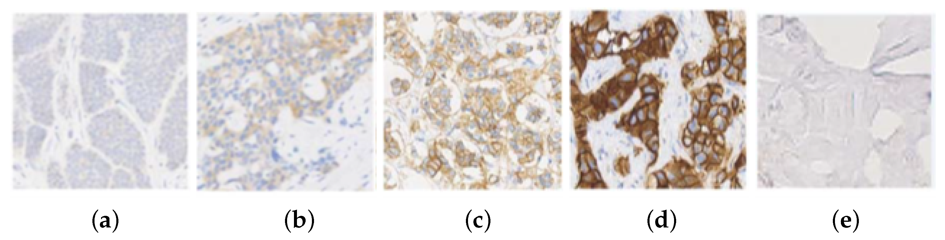
Figure 1.
HER2 images samples and their classification: (a) class 0; (b) class 1; (c) class 2+; (d) class 3+; and (e) Background.
To grade the score in Whole Slide Images (WSI), pathologists follow a diagnosis rule which depends on the total area stained by the biomarker. This is described in Table 1.

Table 1.
HER2 diagnosis rule followed by pathologists.
Unfortunately, HER2 scoring is known for its significant inconsistency between different observers, which is caused by differences in staining techniques among various institutions and the need to visually estimate the intensity of staining within specific percentages of tumour areas [5]. The inter and intra variability in human diagnosis, as well as the heterogeneous colour intensities of the stain applied, makes this problem suitable for an end-to-end deep learning methodology, which can learn features independent from human perception [6,7]. Moreover, the increasing adoption of digital pathology and higher availability of a large number of well-annotated WSIs allows taking advantage of deep learning techniques to train more accurate and robust models [8]. This kind of methods has been proved to increase the pathologists precision and speed in diagnosis, in comparison with non-aided approaches [9,10]. This idea is further supported by studies showing that glass slides and digital images are equally accurate for HER2 interpretation in pathology prognosis [11,12].
HER2 scoring typically involves the classification of small patches extracted from the WSI. These patches are then used to generate predictions at the patch level, which are then aggregated to obtain a prediction for the entire slide. There are two approaches to patch classification: fully supervised and weakly supervised. In fully supervised approaches, the task involves classifying every patch within a segmented region. Weakly supervised methods, based on pathologists’ slide evaluation practices, use models to learn patch selection. According to some authors, the latest methods are limited by the need for patch-level labelling, which is not typically used in clinical evaluation. Other studies find that segmenting infiltrating cancer patches does not affect HER2 scoring, despite potential improvements [5].
In the following we provide a comprehensive review of the research works published from 2018 to 2023, focusing on various techniques used to assess the scoring of Her2. Saha et al. [13] present a deep learning framework (HER2Net) for cell segmentation and patch scoring in HER2-stained breast cancer images. HER2Net uses trapezoidal long short-term memory, spatial pyramid pooling, and convolutional and deconvolutional layers. The framework yields a general precision of 96.64%, an accuracy of 98.33% and an F-score of 96.71% in classifying the cell membrane staining pattern as no staining, faint staining, moderate staining, and strong complete staining. Results were obtained from 752 patches cropped from 79 WSIs. This method published in 2018 [13] achieves the highest accuracy value reported thus far. However, it does not differentiate between the segmentation and classification results. The results are presented by modifying the number of training and test patch images, sometimes even using zero training images, which renders the results unclear. Ultimately, a comprehensive score of the entire WSI is missing.
Cordeiro et al. [14] introduce an automated scoring HER-2 algorithm that relies on colour hand-crafted features and traditional machine learning techniques. This is the initial method for HER2 scoring that does not involve segmentation prior to the classification process. As stated in the literature review, the majority of methods involve segmentation, which is recognised for its tendency to introduce errors in subsequent stages. They claim that their method achieved a 94.12% accuracy rate, without the need for explicit segmentation and extraction of structural properties such as cell nuclei and membrane. In addition, it is completely automated and can effortlessly operate on basic desktop computers.
Khameneh et al. [15] propose a model that involves three main components: (1) classification of the whole slide image (WSI) into stroma and epithelium areas using support vector machine (SVM) classifier; (2) training the model using patches from the epithelial part for segmentation of cell membrane staining patterns; and (3) a scoring mechanism that combines tile results, transferring staining intensities and completeness to align with pathologists’ assessments. Experimental results on 127 slides show an average accuracy of 95% for the segmentation but it shows lower performance on the classification stage with an average accuracy of 87%. This study provides a review of 9 previous methods, with accuracy ranging from 79% to 98%. The utmost accuracy is obtained with Saha et al.’s work, as mentioned earlier [13]. There are only two works that use WSIs. One of them has 86 WSIs [16], while the other one, which is their own work [15], has 127 WSIs. The remaining works uses patches derived from multiple WSIs. The number of patches extracted varies, ranging from 77 patches obtained from 77 WSIs, to 752 patches obtained from 79 WSIs, 1265 patches obtained from 253 WSIs, and 2580 patches obtained from 86 WSIs.
In [17] Kabakçı et al. use colour deconvolution to separate channels, followed by segmentation of cell nuclei and boundaries. Then, hand-crafted cell-based features, reflecting membrane staining intensity and completeness, are extracted. Then, these features are fed into a classical machine learning classifier to determine HER2 scores. The final HER2 tissue score is derived by aggregating the individual cell scores, in accordance with ASCO/CAP guidelines. They also present a review of the same methods as in the previous study [15], but distinguishing between methods that rely on hand-crafted feature extraction and those that use deep learning. They argue that deep learning methods suffer from overfitting to the data, necessitating re-training or re-designing the model when new data is introduced. They claim that the hand-crafted features and classical machine learning approach they propose offer an explainable AI solution without requiring the model to be re-trained. Their average accuracy is 91.43% and their F1-score is 91.81%.
In [18] Chem et al. propose a hierarchical Pathologist-Tree Network (PTree-Net) with multi-instance learning (MIL) to use multi-scale features from the WSI pyramids. The method starts by training the Focal-Aware Module with slide labels to accurately detect and classify diagnostic regions. A Patch Relevance-enhanced Graph Convolutional Network then thoroughly analyses the hierarchical arrangement of multi-scale patches from attentive regions. Finally, tree-based self-supervision fine-tunes PTree-Net to improve representation learning and reduce unimportant patches. This method achieves average values of 89.70% for accuracy, 90.77% of F1-score and 83.34% for MCC with standard deviation of around 1.4 based on 4-fold cross validation on a dataset of 105 WSIs. The model leverages comprehensive information from the entire WSI without requiring hand-crafted features or rules. They combine classes 0 and 1+, and the confusion matrix from PTree-Net’s 4-fold cross-validation shows that it performs well identifying WSIs with a 3+ HER2 score, achieving a classification rate of 95.24%, but performs poorly with a 2+ score, achieving 89.16%. The distinction between 2+ and 0/1+ categories presents difficulties, with 11.99% of 0/1+ samples misclassified as 2+ and 9.38% vice versa.
The approach presented by Pham et al. [5] combines both fully and weakly supervised HER2 scoring paradigms, providing interpretability without the need for extensive expert annotations. Training and evaluation only use patches that cover more than 10% of the surface area affected by invasive carcinoma. This addresses 96% of invasive carcinoma’s surface area in the user-specified ROI. The model attains an F1-score of 78% on the hold-out test set, along with an average precision of 85.4% with very small standard deviation of 0.05. Additionally, the model achieves a Dice score of 0.91 for class 2+ and 3+ slides, while exhibiting lower scores for classes 0 and 1+. They claim that the use of ASCO/CAP clinical guidelines directly in training and testing contributes to the model’s interpretability and alignment with clinical standards.
The work of Bórquez et al. [19] is the first to study the uncertainty in the classification of Her2 histopathological images into the categories of 0, 1+, 2+, and 3+ at the patch level. The process consists of four stages: WSI pre-processing for colour deconvolution, generation of patch dataset, classification based on Bayesian deep learning, and prediction with estimation of uncertainty. The proposed approach integrates deep learning and Monte Carlo Dropout to quantify uncertainty, a factor frequently overlooked in healthcare applications. This method achieves an average accuracy of 89%, precision of 81%, and recall of 74% for tissue-level classification on the dataset of the Her2 challenge contest [16] with 172 WSIs.
In [7] the authors present a novel study by integrating FISH images alongside IHC images during the training phase. The study presents a machine learning model for HER2 classification, based on logistic regression. The model was trained using 393 IHC images to distinguish between upregulated and normal HER2 expression. Pathologists’ diagnoses (IHC only) and final diagnoses (IHC + FISH) were used for training. The IHC model achieved an accuracy of 88%, precision of 89%, and recall of 43%. In comparison, the IHC + FISH classifier achieved an accuracy of 93%, precision of 100%, and recall of 55%. The model exhibited superior performance when trained using IHC + FISH diagnoses, highlighting the significance of subcellular staining patterns in pathological diagnosis prior to FISH consultation, as opposed to overall intensity.
Finally, the work of Che et al. [20] use deep learning to automatically assess breast cancer Her2 WSI scores on 95 IHC section images with labelled tumour areas. The proposed method has three steps. After extracting labelled masks from WSIs, tumour and normal patches were randomly generated to create a probability map. Applying a threshold to the probability map yielded the binary tumour prediction. Finally, a deep learning model (ResNet34) was fed the patches to improve binary classification. WSI test classes were 0, 1+, 2+, and 3+. The results show 73.49% segmentation accuracy and 95.77% precision at the patch level. On the test set, the F1 score is 83.09% and the accuracy is 97.9%. The study acknowledges limitations. First, dye dosage during slicing can cause colour depth inconsistencies. Colour standardisation in deep learning methods improves tumour area identification but increases execution time without substantially affecting IHC score accuracy. Second, the final stage requires domain knowledge for optimal colour threshold selection. They claim that the influence of colour depth on classification results can be mitigated by collecting HER2 slides from multiple centers.
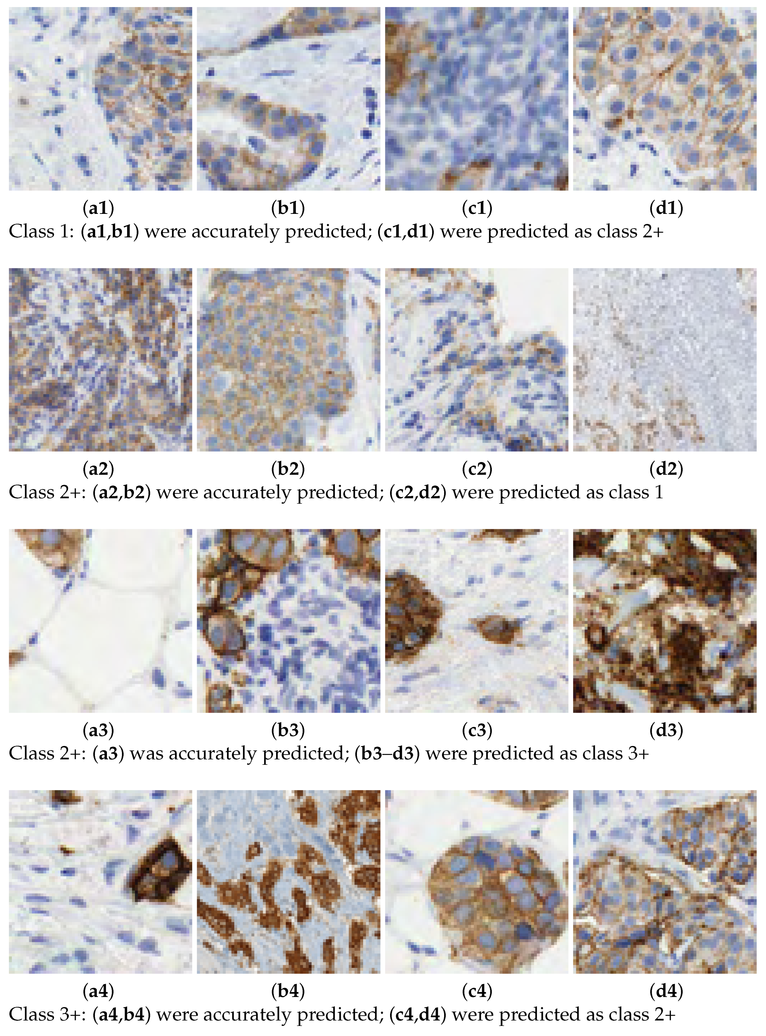
In this work, we aim to overcome the limitations and address the criticisms raised in the aforementioned studies. The entire tissue was divided into patches to mimic the pathologist diagnosis. Then, each patch was classified with a score and, according to the rule described in Table 1, the slide is graded automatically. We introduce a novel 7-class approach. The reason is that the classification in some patches is difficult for class 2+. This is the main source of confusion even for pathologists. See Figure 2 for some examples of 2+ patches and how they can be confused with 1 or 3+ samples. In practice, a 2+ grading prediction is usually equivocal and requires additional tests, such as FISH. The consequences of mixing up these cases, providing an inadequate approach, or failing to address them when required, are significant.

Figure 2.
Scoring HER2 images. Prediction of class labels for various samples.
Once the corresponding datasets for this 7-class configuration are built, five prominent deep neural network (NN) architectures have been considered: AlexNet, GoogLeNet, VGG-16, ResNet-101, and DenseNet-201. To build the dataset for this 7-class configuration, the classification process takes into account the mean confidence of the NN.
To successfully build an accurate deep learning model, a comprehensive and suitable training set is required. Moreover, proper tuning of hyperparameters can enhance and speed up the process. However, a selection of representative data for every class in the problem, even augmenting the available samples with variations and synthetic data, is not always enough to get the expected results. For this reason, this work also performs an ablation study to investigate the performance of the model by applying different data augmentation techniques. Additionally, it is widely acknowledged that colour variation is a pivotal factor in ensuring precise scoring. In order to investigate the generation of new images, we use colour transfer techniques to simulate colour variations.
The proposed method outperforms other existing methods when evaluated using accuracy metrics, establishing its effectiveness in evaluating doubtful cases that lack agreement. The method has been incorporated into a DICOM WSI viewer [21].
The rest of the document is organized as follows. Section 2 details the dataset and how it has been processed. Section 3 describes the implementation details along with the network architectures employed for experimentation. Section 4 provides a description of the outcomes for every different combination of datasets, architectures, and parameters used. Section 5 discusses the insights gained from the experimentation, and highlights its contribution to enhancing the construction of improved models for histopathology scoring. Finally, Section 6 provides a summary of the main findings of this study and outlines potential areas for future research.
2. Materials
2.1. Whole Slide Images
The Whole Slide Images (WSIs) used in this study were generated in the AIDPATH project (http://www.aidpath.eu, accessed on 20 February 2024 ). The dataset consists of 306 WSIs obtained from 153 breast cancer cases at three medical centres, namely Nottingham University Hospital (NHS Trust), Servicio de Salud de Castilla-La Mancha (SESCAM), and Servicio Andaluz de Salud (SAS), as follows:
- NHS: 86 cases of invasive breast carcinomas with 172 WSI.
- SESCAM: 52 cases of invasive ductal carcinomas with 104 WSI.
- SAS: 15 cases of invasive and in situ ductal carcinomas with 30 WSI.
All the slides have the clinical outcome: HER2 negative, positive and equivocal together with the IHC score (0, 1, 2+ or 3+). Table 2 shows the allocation of the 306 WSIs according to their respective score. The distribution of WSIs per class is proportional, with an average of 76 WSIs per class. In order to guarantee the quality of the labels when building the groundtruth in our dataset we carried out a consensus process involving multiple pathologists to score the HER2 images. Pathologists provided the groundtruth at NHS Trust, SESCAM and SAS during standard and quality-measured routine. Each case was reviewed by at least two specialists. The most challenging cases, as well as those lacking agreement, were reviewed by five specialists from the three institutions. If there was a difference in the scoring, the mode was employed. The analysis revealed that there was variability in the scores of the samples in 40% of the cases.
Table 2.
Score-based distribution of the 306 WSIs.
The 86 cases from NHS were used in the HER2 challenge contest [16] as well as other research works [5,13,14,15,17,19,22]. All the WSIs were acquired at 40× magnification. The source of the digital scanning is a Hamamatsu NanoZoomer C9600 (TIF format) for NHS Trust and a Leica DM-4000 (SVS format) for SESCAM and SAS. All the images have an average resolution of 90,000 × 50,000 pixels and 1 GB file size in a proprietary format.
For the purposes of training and evaluating the classification models, 70% of the entire set of WSIs were used for training, while 20% were selected for validation and 10% of the WSIs were specifically chosen as a hold-out test set. The WSIs were partitioned into patches to replicate the pathologist’s diagnosis, as previously stated. Therefore, all the datasets consist of patches of size 64 × 64 pixels that have been extracted from the original slides. These patches are extracted from the left to the right and from the top to the bottom of the image. A stride of 64 pixels is used in both the height and width directions, ensuring that the patches do not overlap.
In the experiments conducted for training and validation, the existing data is augmented and transformed to investigate its intriguing characteristics and obtain more representative datasets. This process enhances the accuracy of the trained models.
2.2. Dataset Building
To maximize the range of input variations for the deep learning workflow, different datasets are built with two different class arrangements as exposed below. Moreover, data augmentation techniques are applied to explore whether the data is suitable enough to learn accurate classification models and how to improve the performance. Two main transforms have been applied for data augmentation:
- Spatial transformations: vertical and horizontal flips and rotations of 90°, 180° and 270°, as shown in Figure 3. In this case the classifier learns invariant orientation features which can help to classify a patch correctly independently of its position on the image.
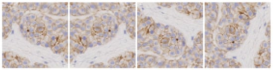 Figure 3. Data augmentation using spatial transformations.
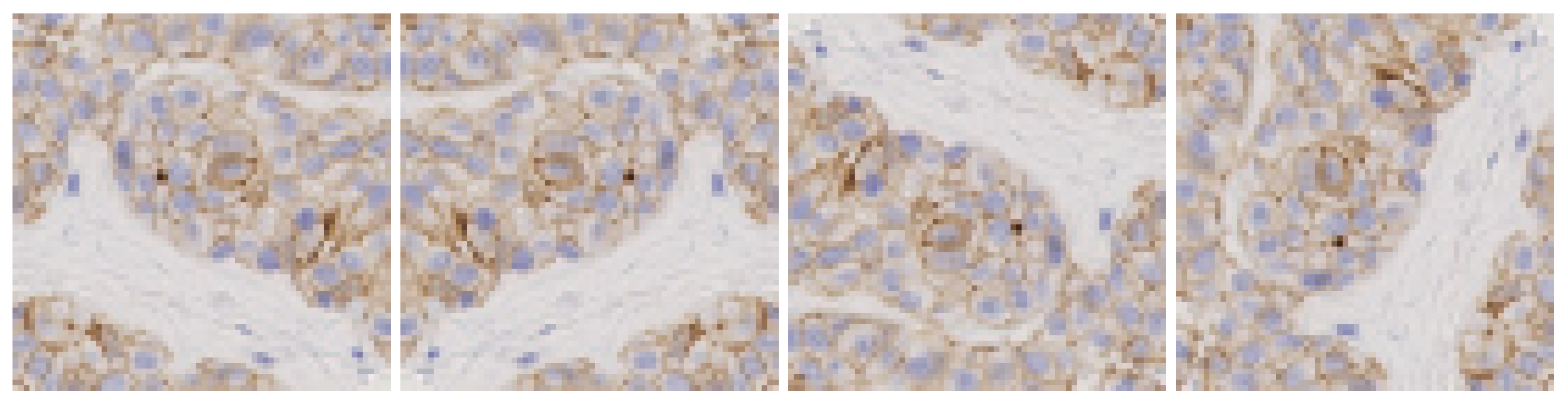
 - Colour transfer: the aim is to artificially produce colour variation patches within the range of colours observed in the different slides. By adapting the colour of one image to another, patches with new colour appearance are generated, as shown in Figure 4.
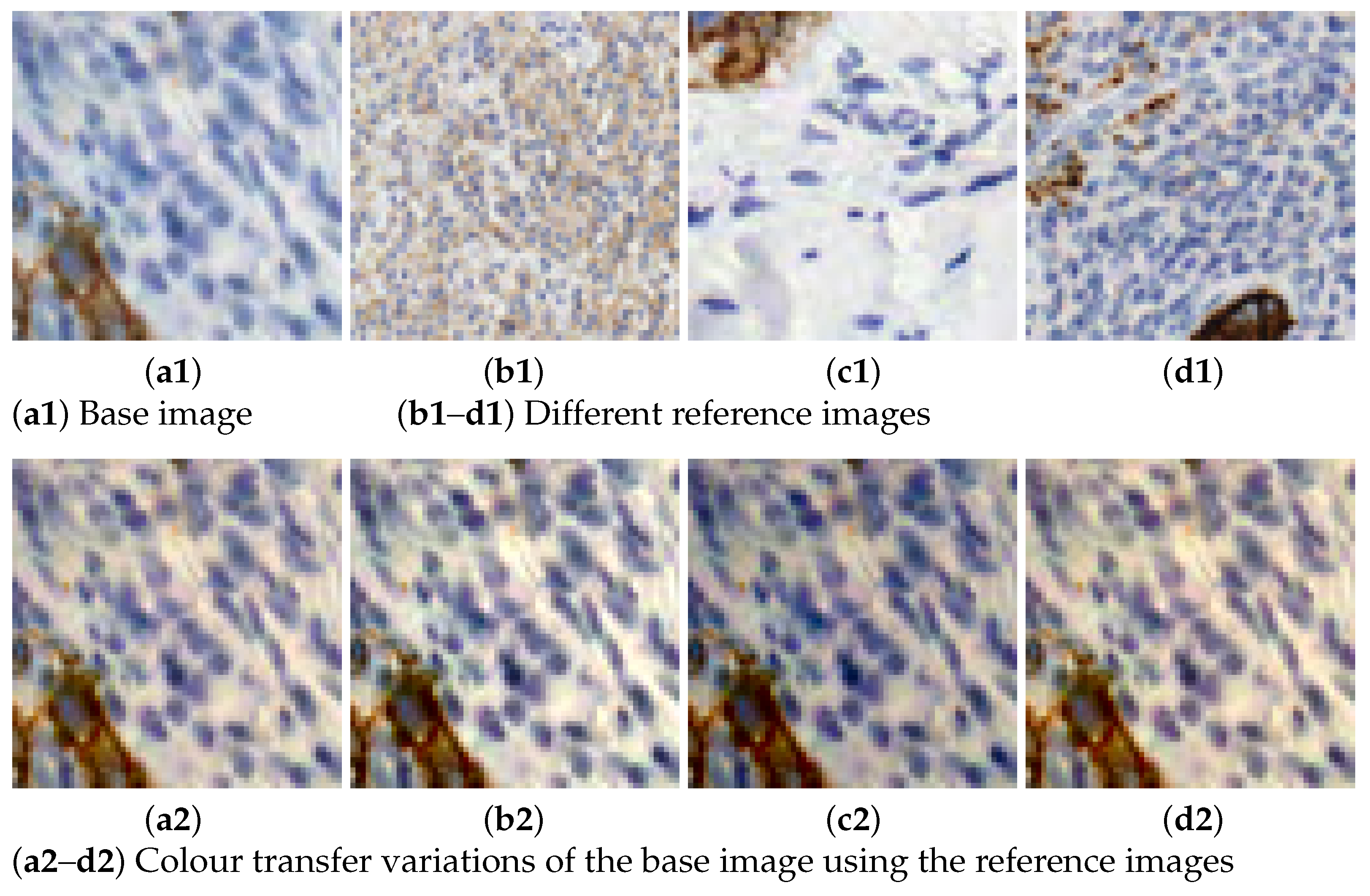
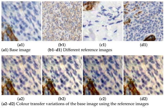 Figure 4. Illustration of the colour transfer results using Macenko’s method.
The use of different biomarkers in digital pathology images often leads to a significant amount of variation in staining. Even for distinct patches that employ the same biomarker [23]. A frequently employed technique for generating additional data involves the aforementioned process of colour transfer. There are different approaches to apply this procedure [24,25,26,27,28,29]. A popular technique, employed in this work, is the one introduced by Macenko in [26]. Our selection is based on the study performed in [30], where the colour consistency and the effectiveness of the Macenko’s method (MM) are measured by computing the colour distance with the NBS metric (National Bureau of Standards), and it was the most suitable to keep a trade-off between these two variables.
The work of Fernández-Carrobles et al. [30] studies four different methods used for colour transfer or colour standardization: histogram matching (HM) [27,28], MM [26], Reinhard’s method (RM) [25] and non-linear spline mapping method (SM) [29]. Results showed that the smallest colour distance is obtained with the SM method. Regarding MM and HM, there is no significant difference as both obtain slightly different colours. The RM method obtained a lower NBS colour distance, but it had a large variability. As for the drawbacks of these methods, RM was affected by the hue and saturation of the source images, while SM was affected by the low contrast of the source images. However, the latter had a better colour consistency. The main drawback of the SM method is the huge computational time required. For these reasons, MM is applied in our work.
MM is applied with 6 different reference colour intensity images to produce variations to the rest of the images. Increasing the number of colour variations helps covering a broader range of cases present in different stain and digitalization processes. Figure 4 shows an example of how this technique is applied in our dataset. There, the reference images with varying intensities are displayed alongside their application to a single sample or base image. The colour varies from darker, lighter to bluish or reddish colours.
The use of data augmentation enables to explore and extract conclusions regarding performance in different training scenarios and the underlying behaviour, as elaborated upon in the discussion Section.
In order to assess the impact of class balance on deep learning training [31], datasets are built with both equal and imbalanced numbers of samples per class. Furthermore, in order to assess the impact of colour variation alone, datasets with and without colour transfer are also examined.
Therefore, we have generated three datasets consisting of five classes each, which we have named DS0, DS1, and DS2. Furthermore, an additional dataset, referred to as DS3, was created by extracting the difficult and challenging cases from the original DS2 dataset. This resulted in a new dataset consisting of seven distinct classes.
A summary of the features of each dataset is shown in Table 3. The exact number of samples for each dataset is shown in Table 4.
Table 3.
Configuration settings for all datasets.
Table 4.
Partitioning of all datasets.
- Five-class dataset
To obtain an accurate evaluation dataset, the initial approach under consideration involves constructing a dataset that encompasses the same number of classes as those considered by the pathologist during the diagnostic process. The groundtruth slides undergo processing based on the patches policy (Table 1), resulting in the extraction of samples. These samples are then categorised into 5 distinct groups based on their associated scores. In this context, each class implies a specific meaning:
- Back. Represents the background, that is a patch with non-tissue regions.
- Class 0. Represents a patch associated to HER2 score 0.
- Class 1. Represents a patch associated to HER2 score 1.
- Class 2+. Represents a patch associated to HER2 score 2+.
- Class 3+. Represents a patch associated to HER2 score 3+.
The following data sets, each containing 5 classes, have been created to address the mentioned issues:
- DS0: is the initial 5-class dataset obtained with patch extraction from the original slides and groundtruth. As the presence of positive grading samples (classes 2+ and 3+) is less common than negative and background samples (classes 0, 1 and background), this dataset is unbalanced and has fewer samples for these classes, as shown in Table 4.
- DS1: a 5-class dataset is built only with spatial transformations (rotations, flips) to reach 50,000 samples per class. In this way, the influence of these techniques to produce augmented data is tested.
- DS2: this dataset has the same number of samples per class as DS1, but they have been chosen randomly from spatial transformations and colour transformations too. Therefore, the patches included in this dataset do not only contain rotations and flips but also colour variations of these. This way a wider range of stains is covered, and its influence, with the same number of samples, can be observed.
- Seven-class dataset
In a different configuration of the problem, we employ the novel subclass approach, consisting of 7 classes. As mentioned in the introduction, 2+ is the most pertinent and challenging class. Therefore, it was decided to split these samples into two intermediary categories to reduce erroneous classifications. The result of the DS2 classification was used in this process, by assessing both confidence and prediction, as elaborated in the next sections. Furthermore, pathologists conducted additional validation of these results. The ultimate classification of the complete WSI entails combining the group of patches rated 1.5 into the 2+ outcomes, and conversely, the patches rated 2.5+ are incorporated into the 3+ score. Thus, the outcome is generated in accordance with the protocol established by the pathologist. As a result, the 7-class definition comprises two more classes in addition to the aforementioned 5-class for 0, 1, 2+, and 3+, that is:
- Class 1.5. Represents patches whose diagnosis is not clearly 1 or 2+, so they are highlighted to be categorized by the pathologist.
- Class 2.5+. Represents patches whose diagnosis is not clearly 2+ or 3+, so they are highlighted to be categorized by the pathologist.
A dataset consisting of 7 classes has been built to encompass the described aspects:
- DS3: this dataset follows the same approach as DS2 but with the 7-class subdivision. With this dataset we can assess whether the combination of the split classes along with the spatial and colour transformations enhances the results.
The number of samples in each fold (training, test, and validation) and grading class are shown in Table 4. For the DS0 dataset, 100 patches per class are reserved for testing while the rest are used for training and validation (performed each epoch) in a 90–10% proportion. For DS1, DS2 and DS3, as the number of samples is higher, 1000 samples per class are employed for testing, while training-validation follows the same schedule. Data augmentation was performed to the training and validation folds.
The datasets will be used to train various network architectures with optimised parameters in order to maximise performance. This will allow us to evaluate how certain techniques or structures contribute to improved accuracy in patch classification, ultimately leading to improved HER2 grading and diagnosis.
3. Methods
To develop an efficient computer vision workflow based on deep learning methodos, a comprehensive study and experimentation of different neural network architectures and settings is needed. Thus, five different CNNs(Convolutional Neural Networks) and parameter settings have been tested. These architectures, as well as the implementation details, are explained in the following subsections and summarized in Table 5.
These architectures were chosen to compare the proposed methodology to existing methods for HER2 scoring. The AlexNet, GoogleNet and VGG networks were selected due to their simplicity and prior use in the HER2 challenge [16]. The remaining networks, ResNet and DenseNet were selected based on their ability to offer new attributes, achieving good results while maintaining a trade-off between computational time and workload. In addition, ResNet has been frequently used for HER2 scoring in breast cancer [18,20,22] and more recently for predicting the HER2 status in oesophageal cancer [32]. Moreover, DenseNet has also been employed recently for HER2 scoring in breast cancer [5].
Table 5.
Summary of the NN architectures used and implementation details.
Table 5.
Summary of the NN architectures used and implementation details.
| Network | Release | Parameters | Main Feature |
|---|---|---|---|
| AlexNet [33] | ILSVRC 2012 | 60 | Ad-hoc architecture |
| GoogleNet [34] | ILSVRC 2014 | 7 Millions | Inception module |
| VGG-16 [35] | ILSVRC 2014 | 138 | 5 Millions Conv-3 × 3 blocks |
| ResNet-101 [36] | ILSVRC 2015 | 45 Millions | Residual maps |
| DenseNet-201 [37] | ILSVRC 2016 | 20 Millions | Dense blocks |
3.1. AlexNet
This network architecture was one of the first developed for deep learning. It was the winner of the ILSVRC in 2012, which is one of the most challenging computer vision competitions. There, the algorithms and models try to distinguish among 1000 different classes of familiar objects, like several kinds of dogs, cats, trees and more common entities.
The main novelty introduced by AlexNet was the use of convolution layers, which are designed to modify the dimensionality of the input. As stated in [33] it contains 60 million parameters (connections and weights among neurons) to be learned during training.
The AlexNet architecture includes five convolutional layers each followed by pooling and, finally, two fully convolutional layers. There is no basic building block (a building block here means, the smallest unit which is repeated throughout the network) since this network was one of the very first concepts of deep learning applied to images. As a result, there was yet no standard about filter sizes (size of convolution step) to be used or how many convolutions, and everything was figured out by experimentation.
The AlexNet network is meant to provide an entry point in experimentation. More advanced networks such as GoogleNet, VGG-16, ResNet-101 and DenseNet-201 will assumably improve the performance regardless of applying data augmentation techniques. This is because their deeper layers and structures are able to learn more advanced and complex features in comparison [38].
3.2. GoogLeNet
Proposed in [34], it was the winner of ILSVRC 2014. An inception module is the basic building block of the network. In short, the inception module does multiple convolutions, with different filter sizes, as well as pooling in one layer. As a result, instead of having us decide when to use which type of layer for the best result, the network automatically figures this out after training (avoiding experimental ad-hoc architecture exploration as in the AlexNet network).
It uses combinations of inception modules, each including some pooling, convolutions at different scales and deep concatenation. It also uses 1 × 1 feature convolutions that work like feature selectors. In comparison with AlexNet, the number of parameters is reduced to 7 million. It performs 8520 million floating point operations per forwarding pass.
3.3. VGG-16
This network was developed for ILSVRC 2014 too, proposed in [35]. Their concept brought some standards: it was suggested that all filters should have a size of 3 × 3, poolings should be placed after every 2 convolutions, and the number of filters should be doubled after each pooling. As a result, its building block consists of two convolutional layers followed by a pooling layer. This block is repeated 5 times consecutively. The rest of the network performs two fully connected layers with a 50% dropout each and, finally, a classification layer with the output classes probability.
In this case, the objective was to get the best feature extractor possible, although a deeper network means a slower one. It contains 138 million parameters to be learned, which is twice the amount used in AlexNet and near 20 times in comparison with GoogleNet, performing 30,690 million floating point operations in a single inference.
3.4. ResNet-101
This architecture was presented in the ILSVRC competition in 2015 and described in [36]. It introduced what is known as residual maps, in which information from the previous layer is added in later ones. Thus, it is possible to acquire correlated features through element-wise addition while bypassing the layers in the path via “shortcut” connections. The idea is motivated by the degradation problem (training error increases as depth increases). If further layers can be constructed using identity mappings from the previous layers, a deeper model should have training error no higher than its shallower counterpart, but with the accuracy gains from increased depth. This network contains 45 millions of parameters.
3.5. DenseNet-201
Presented in the ILSVRC competition in 2016, the DenseNet architecture was developed in [37]. Increasing the depth of the convolutional neural network caused a problem of vanishing information about the input or gradient when passing through many layers. To solve this, the authors introduced an architecture with simple connectivity pattern to ensure the maximum flow of information between layers both in forward computation as well as in backward gradients computation. This network connects all layers in such a way each layer obtains additional inputs from all other layers and passes its feature-maps to all subsequent layers, that is it obtains diversified features with the channel-wise concatenation.
In the network, each layer implements a non-linear transformation, which can be a composite function of operations such as Batch Normalization (BN), Rectified Linear Unit (ReLU), pooling or convolution. These multiple densely connected blocks are the basic building blocks of this network. Finally, they are connected with transition layers which perform convolution and pooling. Although it has more connections than others, its design makes it optimum in the number of parameters, with “only” 20 million.
4. Results
Once the 5-class datasets are built, each architecture network is trained and validated. Table 6 and Table 7 show a summary of the results for all the methods and datasets.
Table 6.
Results of sensitivity (Sens), specificity (Spec) and accuracy (Acc) for the five-class datasets. Each column depicts an architecture: AlexNet (AN), GoogleNet (GN) and VGG-16 (VGG).
Table 7.
Results of sensitivity (Sens), specificity (Spec) and accuracy (Acc) for DS2. Each column depicts an architecture: ResNet-101 (RN) and DenseNet-201 (DN). The best results are highlighted in bold.
In all the experiments, the same set of hyperparameters was used so that performance can be compared in the same conditions. These parameters for training have been chosen considering two principles in mind. First, this is a finetuning over previously ImageNet trained models. Second, that reproducibility over different networks is desirable. Because of that, L2 regularization and gradient clipping are defined. The specific values have been chosen from the common range that they take from the state of the art so that they can work in a large range of models with no issue. These references provide more details about how they are defined and how they should be used [39,40,41]. Nevertheless, no noticeable differences should be observed given that the parameters are set within the proper range.
Regarding the amount of data of these datasets, 3 epochs are enough to adapt the network to the problem. This is observed in the training plots of the loss function, since after the third epoch the network training was stable and no improvement was observed. To further prevent overfitting and to refine the model weights during these epochs, a learning rate decay is also applied, which is common in the state of the art to reduce the magnitude of weight changes throughout the learning process.
As a result, these are the specific parameters: training was carried out during 3 epochs, using ImageNet initialization weights, with 0.01 as the initial learning rate and a decay of 0.1 at each epoch for training stabilization. Gradient clipping (L2 normalization method) with a 0.05 threshold was used to prevent gradient exploding. Momentum at 0.9 and L2 regularization at 0.004 are also applied to avoid overfitting.
The most optimal performance is observed with the ResNet and DenseNet models, and with the DS2 dataset where data augmentation and balanced classes are implemented. Detailed remarks regarding the experiments conducted on each dataset are as follows:
- DS0: The experiments for this dataset gave low sensitivity results for 1 and 2+ classes (the best are 0.84 for VGG in 1, and 0.82 for DenseNet in 2+). However, the negative class (0) is well classified by all methods (sensitivity ranges from 0.93 to 0.95). For class 3+, ResNet is able to get promising results (0.89 sensitivity) even though it is the class with fewer samples available.
- DS1: With this augmented dataset, the performance is in general increased for the key classes in diagnosis (2+ and 3+). For 2+, the best results are shown by VGG (0.88 sensitivity) and DenseNet (0.85). However, the less complex models, such as Alexnet and GoogleNet, slightly degrade their performance.
- DS2: This dataset, apart from spatial augmentation, also introduces colour variations with the Macenko method. The ResNet model increases its performance, but DenseNet consolidates as the best model for the 5-classes datasets, with an average sensitivity of 0.88 for these classes. Additionally, Table 8 shows the mean confidence values for the test set of the DS2 dataset using ResNet and DenseNet models. It shows that DenseNet classifies with a greater level of confidence. The confusion matrix for the experiment with this model is shown in Table 9, illustrating the performance of each class. The classification model’s metrics, including sensitivity, specificity, precision, accuracy, F1-score, and Matthews Correlation Coefficient (MCC), are shown in Table 10.
Table 8. Mean confidence values for the test set of DS2 using ResNet-101 and DenseNet-201 models. The best results are highlighted in bold.
Table 9. Confusion matrix for DenseNet-201 applied to DS2 dataset with 5 classes.
Table 10. Metric values per class for DenseNet-201 applied to DS2 dataset with 5 classes.
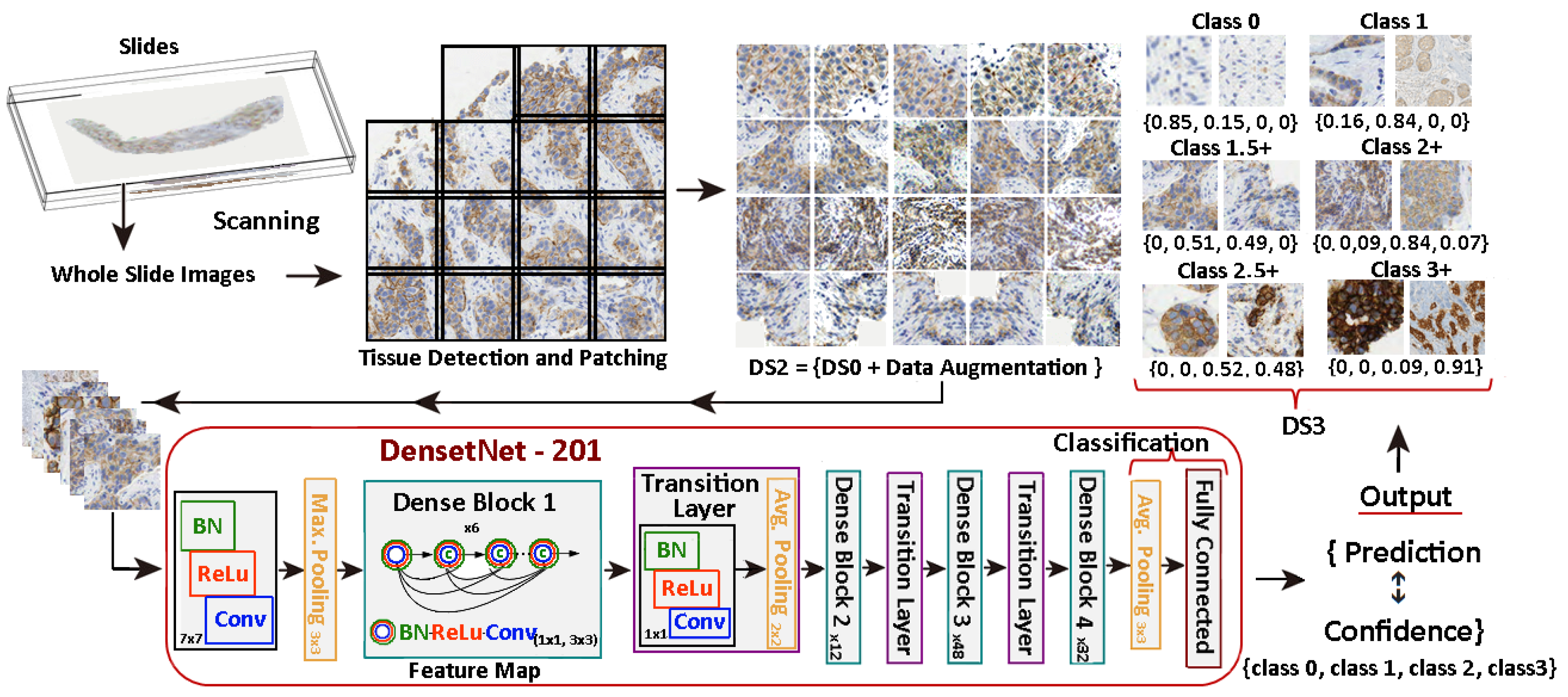
The DS3 dataset, consisting of 7 classes, has been generated using the prediction and confidence values obtained from the DenseNet-101 model applied to the DS2 dataset. Figure 5 illustrates the process.
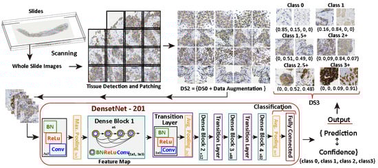
Figure 5.
Generation of DS3 dataset with 7-classes using DenseNet-101 applied to DS2.
Once the DS3 dataset is generated, the experimentation process done is similar to the previous one. The idea behind this subdivision is to improve the performance for the most critical classes (2+ and 3+) since they are determinant for the diagnosis and treatment. The experiments demonstrated that ResNet and DenseNet remained the most effective networks. Specifically, when applied to this dataset, the performance of these two deep models exhibited significant improvement, their interpretation is provided below:
- DS3: with this dataset, the novel 7-class approach is tested together with all the data augmentation proposed, that is spatial augmentation (rotations and flips) and colour variations. The ResNet model achieves the overall highest mean sensitivity for the experimentation with the highest confidence values (see Table 11). The confusion matrix for the experiment with the ResNet-101 model is shown in Table 12. This table shows the results for the proposed classes that have been trained to enhanced scoring for difficult patches (1.5 and 2.5+). The classification model’s metrics, including sensitivity, specificity, precision, accuracy, F1-score, and MCC, are shown in Table 13.
Table 11. Mean confidence values for the test set of DS3 using ResNet-101 and DenseNet-201 models. The best results are highlighted in bold.
Table 12. Confusion matrix for ResNet-101 applied to DS3 dataset with 7 classes.
Table 13. Metric values per class for ResNet-101 applied to DS3 dataset with 7 classes.
Afterwards, the aggregation process is performed so that each cell in the confusion matrix is added to the corresponding class it is associated to (2+ for 1.5 and 3+ for 2.5+). This aggregation allows for the restoration of the scoring scheme for pathology diagnosis, which is based on 5 classes, and enables the evaluation of its effective performance. Table 14 shows the confusion matrix of the classification when combining the intermediate classes (1.5 and 2.5+) with their respective true classes (2+ and 3+). The classification model’s metrics, including sensitivity, specificity, precision, accuracy, F1-score, and MCC, are shown in Table 15. By employing this methodology, the accuracy of the 2+ class is enhanced to 96%, while the 3+ class achieves a remarkable 98% accuracy.
Table 14.
Confusion matrix for ResNet-101 in DS4 aggregating to 5 classes.
Table 15.
Metrics Values per Class for ResNet in DS3 aggregating to 5 classes.
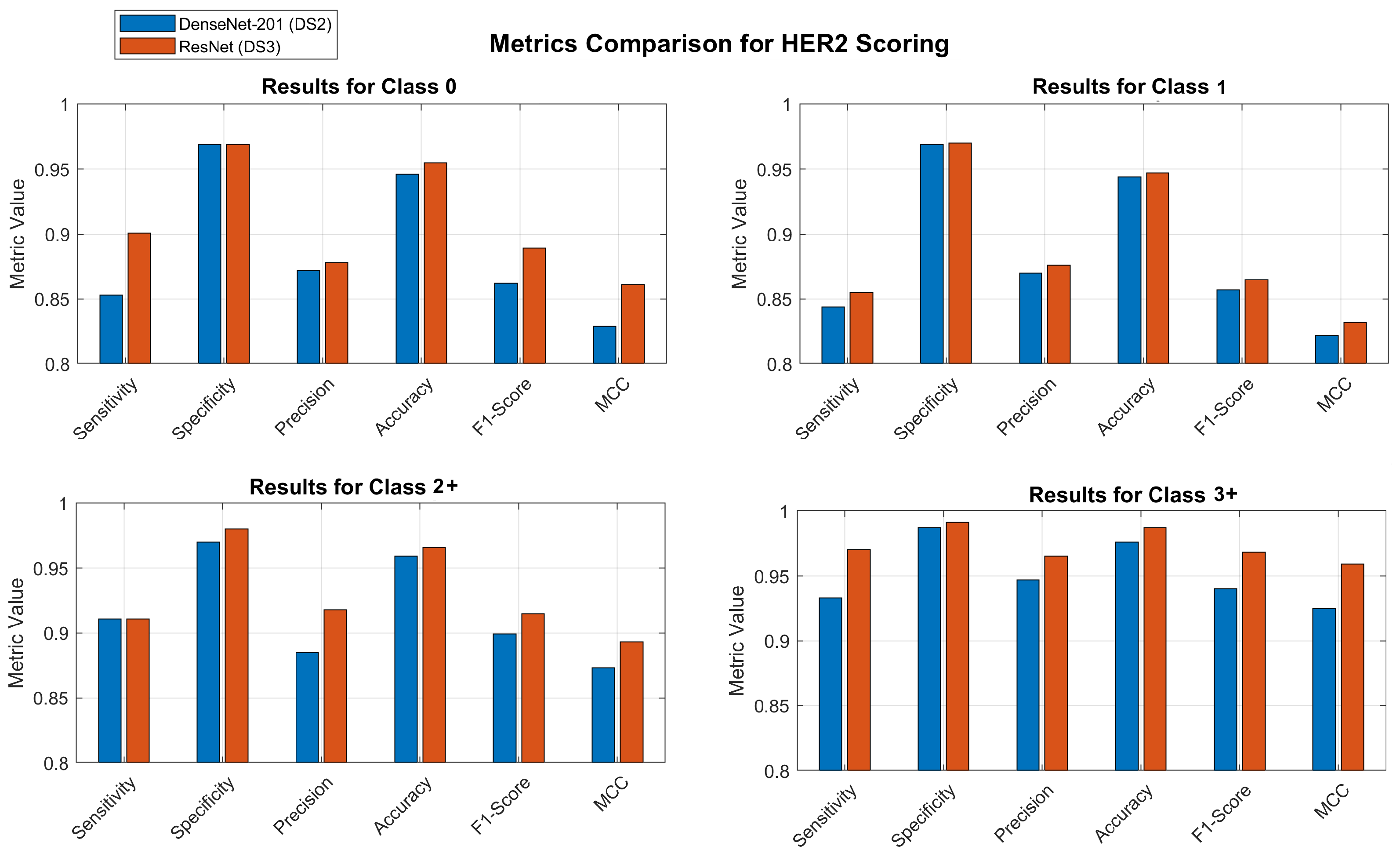
Figure 6 shows the bar charts to compare all the metrics for the two classification models, that is, directly classifying in 5 classes, and classifying in 7 classes and then aggregating the results into 5 classes. The comparison is displayed for each individual class. To illustrate the distinctions, the abscissa axis of the bar charts is set at 0.80.
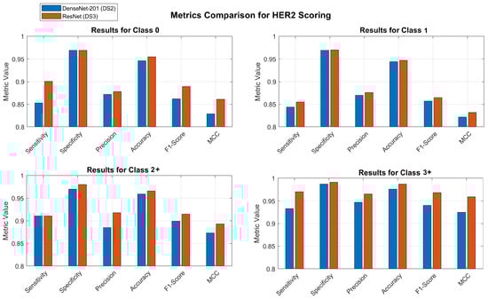
Figure 6.
Comparison of models. Blue bars show the results when classifying directly into 5 classes and red bars show the results when classifying into 7 classes and aggregating to 5 classes.
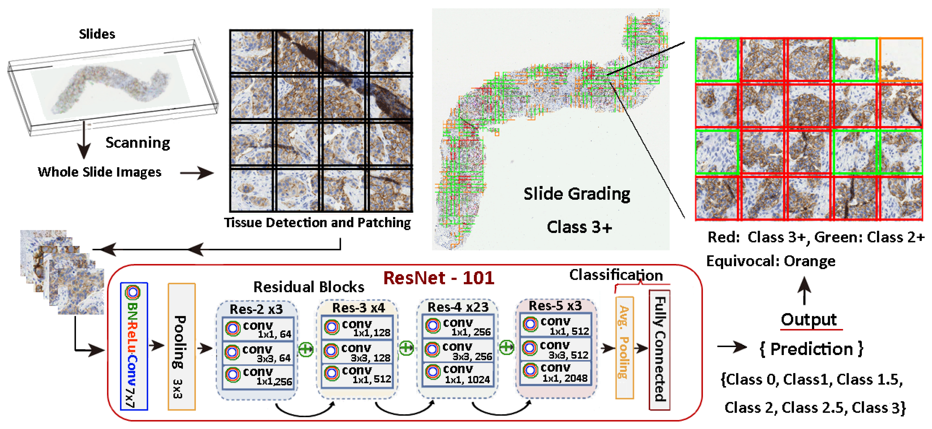
Figure 7 illustrates the entire process and it shows an example of a slide patch classified using a model trained with the methods stated in this work. There, the relevant tissue regions are highlighted in different colours depending on their score and influence in the grading decision. In this specific case, a 9.76% of the tissue is reported as 3+, so the system evaluates the slide as a 3+ positive, providing a warning to check for equivocal tissue regions for further analysis by the pathologist.
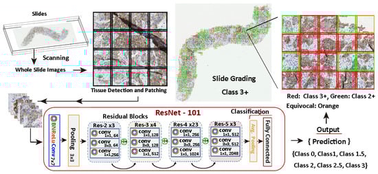
Figure 7.
HER2 scoring procedure. The workflow involves a 7-class classification and a 5-class aggregation process.
Comparing the outcomes achieved using the proposed method to those cited in the current literature [13,14,15,16,17,18,19,20], a comparison can be drawn with the outcomes of five of the mentioned methods, all of which used the AIDPATH database [14,15,16,17,19]. Among these, Cordeiro et al. [14] reported the highest accuracy rate of 94%. When comparing with the approach proposed by Chem et al. [18], which utilises MIL at the pyramidal level, the obtained results are consistent with the previously reported findings, achieving an accuracy of approximately 91%. These results may be attributed to the network’s lack of access to supplementary texture or tumour microenvironment data, instead relying on the same information presented at a varying scale. Finally, when we apply the ResNet34 network used in Che et al. [20] to our dataset, the results are comparable to those previously reported, with an average accuracy of 94%. Thus, the proposed method outperforms other existing methods, as proven by the obtained results with an average accuracy of 97%.
5. Discussion
This section presents a discussion of our findings, with a particular focus on analyzing the influence that different architectures and augmentation techniques have on performance. In addition to this, it provides an analysis of the strategy of dividing the classes that are the most uncertain in order to establish a distinct decision boundary.
The preliminary tests conducted with DS0 have produced encouraging results and laid the groundwork for further comparisons with various configurations in the future. First, the process of augmentation begins with spatial transformations, which are then followed by the application of color transfer in order to improve the results. Through the utilization of this dual approach, the dataset is subjected to a greater degree of staining variation, which ultimately leads to an improvement in performance across all models operating within the 5-class classification. The ResNet and DenseNet models, which are the most complex, also demonstrate improved performance in the 7-class classification. This is a significant finding.
The results of our experiments demonstrate that augmentation and balancing techniques are essential for achieving stable and consistent results across all models. This highlights the significance of balancing as an essential component for efficient learning. A reduction in the risks of overfitting is achieved through the utilization of these methodologies, which ultimately results in improved outcomes for classes that are underrepresented. It is important to highlight the robust and dependable nature of these techniques by mentioning the performance improvement that was observed simultaneously across all classes and models.
Upon comparing confusion matrices with the traditional 5-class approach, it becomes clear that the innovative 7-class approach has a number of advantages that are readily apparent. The ambiguous grading decisions and treatment prognosis are significantly impacted as a result of this. According to the ResNet model that makes use of DS3 and the 7-class approach, the sensitivity for classes 2.5+ and 3+ is 95.2% and 96.1%, respectively. When these sensitivities are combined in the aggregated 3+ class, the overall sensitivity reaches 97%. DenseNet demonstrates a sensitivity of 93% for class 3+ when it is applied to DS2. Comparing the 7-classes approach aggregated to the 5-classes for class 2+, it reveals that the former exhibits a 3% greater sensitivity than the latter, using the same model. The ResNet model demonstrated a sensitivity of 88% when evaluated on a dataset with 5 classes. However, when the model was tested on a dataset with 7 classes and the results were aggregated to 5 classes, the sensitivity improved to 91%. The level of variation in class 1 is significantly higher, increasing by 11.5%. Thus, the sensitivity of class 1 when applied to the 5-classes DS2 dataset is 74%. However, the proposed approach using ResNet achieves a sensitivity of 85.5%.
The level of confidence that is associated with the classifications that are made by the model is another important factor that should be taken into consideration. In general, models that are more accurate tend to demonstrate a higher level of confidence. To be more specific, the data presented in Table 8 and Table 11 indicates that DS3 generates a higher level of confidence in comparison to DS2, particularly for our most advanced models. Because of this, the 7-class method provides advantages not only in terms of sensitivity but also in terms of the levels of confidence it provides. According to the results of our experiments, the ResNet model in DS3 is the one that performs the best when it comes to HER2 prediction. In general, it demonstrates a high level of sensitivity (91%), and it also demonstrates higher levels of confidence, ranging from 87% to 97%. In contrast, the DenseNet model is a little bit behind the curve, with confidence levels ranging from 84% to 92%.
A crucial factor to take into account in the proposed approach is the need to conduct tests in the context of clinical practice, utilising a larger dataset and within a constrained timeframe. Considering the computational time is crucial, as the networks that yield the best results are the ones that require more computational time. It is advisable to opt for models that are both lightweight and have a higher speed. Alternatively, in order to enhance the outcomes, it is also possible to analyse and evaluate the tumour microenvironment by considering data from various regions of the WSI, rather than solely focusing on the specific patch that needs to be classified. Therefore, it is worth considering architectures that are built upon transformers. In addition, future research may also consider to develop models that demonstrate greater accuracy in predicting confidence levels for specific categories. The application of an ensemble of networks to enhance the overall performance and, as a result, reduce the reliance on a single model is one method that can be used to accomplish this goal.
6. Conclusions
The main insights that can be extracted from our work, as discussed above, point out that balancing the number of samples per class is key to obtain stable results. Furthermore, the incorporation of colour variations enhances performance, particularly in the deeper networks, which can leverage this newfound knowledge to a greater extent.
Moreover, the novel 7-class approach is considered an improvement over the results, as it enables the identification and isolation of equivocal and challenging patches for subsequent revision, while simultaneously improving the precision of automated grading.
The proposed method eliminates the need for a segmentation stage and surpasses the performance of other existing methods. The final results of the aggregation process show an average accuracy of 97%, an F1-score of 92%, a Matthews correlation coefficient of 90%, and an average precision of 92%.
Regarding future work, the implementation of an application relying on these experiments should consider other aspects of the models apart from performance. For example, in a grading application that performs the scoring within a scanner using a general purpose computer, the Googlenet or ResNet models are more suitable for deployment and represent the best trade-off network. This is because they are lighter and faster than VGG-16 or DenseNet-201, for example, which are the most computationally expensive. Moreover, the 7-class approach allows the model to deal with doubtful patches, which are isolated in specific classes that are designed to warn the pathologists to take them in special consideration.
Taking into account the confidence in prediction, further work may consider models that are more reliable to specific classes, so that ensemble trees of networks could be developed to enhance the performance rather than relying on a single model.
Author Contributions
A.P. made the implementation, conducted the experiments, and contributed to the preparation of the original draft. L.G. curated the data and evaluated the models. O.D. analysed the results and contributed to the writing of the document. G.B. supervised the entire project, conceptualised it, and conceived the experiments. The manuscript was reviewed by all authors. All authors have read and agreed to the published version of the manuscript.
Funding
This work has been funded by the European FEDER fund, and the HANS project (Project Reference: PID2021-127567NB-I00) supported by the Spanish Ministry of Science, Innovation, and Universities.
Data Availability Statement
The datasets used and/or analysed during the current study will be available upon request to the corresponding author. Accession codes: The code implemented during the current study will be also available upon request to the corresponding author.
Acknowledgments
The authors acknowledge support from the European Union FP7 programme under grant agreement No. 612471 (http://aidpath.eu/, accessed on 20 February 2024) and the participation of the clinical centres. This project has enabled us to gather and assess all the datasets used in this project.
Conflicts of Interest
The authors declare no conflict of interest. The funders had no role in the design of the study; in the collection, analyses, or interpretation of data; in the writing of the manuscript; or in the decision to publish the results.
Abbreviations
The following abbreviations are used in this manuscript:
| American Society of Clinical Oncology | ASCO |
| BN | Batch Normalization |
| College of American Pathologists | CAP |
| FISH | Fluorescence in situ Hybridization |
| HER2 | Human Epidermal Growth Factor Receptor 2 |
| IHC | Immunohistochemical |
| MCC | Matthews Correlation Coefficient |
| NBS | National Bureau of Standard |
| NN | Neural Network |
| SVS | ScanScope Virtual Slides |
| SVM | Support Vector Machine |
| TIF | Tagged Image File Format |
| WSI | Whole Slide Image |
References
- Taylor, C.R.; Rudbeck, L. Education Guide-Immunohistochemical Staining Methods; Dako Denmark A/S: Glostrup, Denmark, 2013. [Google Scholar]
- Wolff, A.C.; Hammond, M.E.H.; Allison, K.H.; Harvey, B.E.; Mangu, P.B.; Bartlett, J.M.; Bilous, M.; Ellis, I.O.; Fitzgibbons, P.; Hanna, W.; et al. Human epidermal growth factor receptor 2 testing in breast cancer: American Society of Clinical Oncology/College of American Pathologists clinical practice guideline focused update. Arch. Pathol. Lab. Med. 2018, 142, 1364–1382. [Google Scholar] [CrossRef]
- Perez, E.A.; Romond, E.H.; Suman, V.J.; Jeong, J.-H.; Sledge, G.; Geyer, C.E., Jr.; Martino, S.; Rastogi, P.; Gralow, J.; Swain, S.M.; et al. Trastuzumab plus adjuvant chemotherapy for human epidermal growth factor receptor 2–positive breast cancer: Planned joint analysis of overall survival from NSABP B-31 and NCCTG N9831. J. Clin. Oncol. 2014, 32, 3744–3752. [Google Scholar] [CrossRef]
- Baez-Navarro, X.; van Bockstal, M.R.; Nawawi, D.; Broeckx, G.; Colpaert, C.; Doebar, S.C.; Hogenes, M.C.; Koop, E.; Lambein, K.; Peeters, D.J.; et al. Interobserver Variation in the Assessment of Immunohistochemistry Expression Levels in HER2-Negative Breast Cancer: Can We Improve the Identification of Low Levels of HER2 Expression by Adjusting the Criteria? An International Interobserver Study. Mod. Pathol. 2023, 36, 100009. [Google Scholar] [CrossRef]
- Pham, M.D.; Balezo, G.; Tilmant, C.; Petit, S.; Salmon, I.; Hadj, S.B.; Fick, R.H. Interpretable HER2 scoring by evaluating clinical guidelines through a weakly supervised, constrained deep learning approach. Comput. Med. Imaging Graph. 2023, 108, 102261. [Google Scholar] [CrossRef]
- Kabir, S.; Vranic, S.; Mahmood Al Saady, R.; Salman Khan, M.; Sarmun, R.; Alqahtani, A.; Abbas, T.O.; Chowdhury, M.E. The utility of a deep learning-based approach in Her-2/neu assessment in breast cancer. Expert Syst. Appl. 2024, 238, 122051. [Google Scholar] [CrossRef]
- Cordova, C.; Muñoz, R.; Olivares, R.; Minonzio, J.G.; Lozano, C.; Gonzalez, P.; Marchant, I.; González-Arriagada, W.; Olivero, P. HER2 classification in breast cancer cells: A new explainable machine learning application for immunohistochemistry. Oncol. Lett. 2023, 25, 1–9. [Google Scholar] [CrossRef] [PubMed]
- Komura, D.; Ishikawa, S. Machine learning methods for histopathological image analysis. Comput. Struct. Biotechnol. J. 2018, 16, 34–42. [Google Scholar] [CrossRef]
- Steiner, D.F.; MacDonald, R.; Liu, Y.; Truszkowski, P.; Hipp, J.D.; Gammage, C.; Thng, F.; Peng, L.; Stumpe, M.C. Impact of deep learning assistance on the histopathologic review of lymph nodes for metastatic breast cancer. Am. J. Surg. Pathol. 2018, 42, 1636–1646. [Google Scholar] [CrossRef] [PubMed]
- Jain, E.; Patel, A.; Parwani, A.V.; Shafi, S.; Brar, Z.; Sharma, S.; Mohanty, S.K. Whole Slide Imaging Technology and Its Applications: Current and Emerging Perspectives. Int. J. Surg. Pathol. 2023. Online ahead of print. [Google Scholar] [CrossRef]
- Wilbur, D.C.; Brachtel, E.F.; Gilbertson, J.R.; Jones, N.C.; Vallone, J.G.; Krishnamurthy, S. Whole slide imaging for human epidermal growth factor receptor 2 immunohistochemistry interpretation: Accuracy, Precision, and reproducibility studies for digital manual and paired glass slide manual interpretation. J. Pathol. Inform. 2015, 6, 22. [Google Scholar] [CrossRef] [PubMed]
- Evans, A.J.; Brown, R.W.; Bui, M.M.; Chlipala, E.A.; Lacchetti, C.; Milner, D.A.; Pantanowitz, L.; Parwani, A.V.; Reid, K.; Riben, M.W.; et al. Validating Whole Slide Imaging Systems for Diagnostic Purposes in Pathology: Guideline Update From the College of American Pathologists in Collaboration With the American Society for Clinical Pathology and the Association for Pathology Informatics. Arch. Pathol. Lab. Med. 2021, 146, 440–450. [Google Scholar] [CrossRef]
- Saha, M.; Chakraborty, C. Her2Net: A Deep Framework for Semantic Segmentation and Classification of Cell Membranes and Nuclei in Breast Cancer Evaluation. IEEE Trans. Image Process. 2018, 27, 2189–2200. [Google Scholar] [CrossRef]
- Cordeiro, C.Q.; Ioshii, S.O.; Alves, J.H.; Oliveira, L.F. An automatic patch-based approach for her-2 scoring in immunohistochemical breast cancer images using color features. arXiv 2018, arXiv:1805.05392. [Google Scholar]
- Khameneh, F.D.; Razavi, S.; Kamasak, M. Automated segmentation of cell membranes to evaluate HER2 status in whole slide images using a modified deep learning network. Comput. Biol. Med. 2019, 110, 164–174. [Google Scholar] [CrossRef]
- Qaiser, T.; Mukherjee, A.; Reddy Pb, C.; Munugoti, S.D.; Tallam, V.; Pitkäaho, T.; Lehtimäki, T.; Naughton, T.; Berseth, M.; Pedraza, A.; et al. HER2 challenge contest: A detailed assessment of automated her 2 scoring algorithms in whole slide images of breast cancer tissues. Histopathology 2018, 72, 227–238. [Google Scholar] [CrossRef]
- Kabakçı, K.A.; Çakır, A.; Türkmen, İ.; Töreyin, B.U.; Çapar, A. Automated scoring of CerbB2/HER2 receptors using histogram based analysis of immunohistochemistry breast cancer tissue images. Biomed. Signal Process. Control 2021, 69, 102924. [Google Scholar] [CrossRef]
- Chen, Z.; Zhang, J.; Che, S.; Huang, J.; Han, X.; Yuan, Y. Diagnose like a pathologist: Weakly-supervised pathologist-tree network for slide-level immunohistochemical scoring. In Proceedings of the AAAI Conference on Artificial Intelligence, Virtual Event, 19–21 May 2021; Volume 35, pp. 47–54. [Google Scholar]
- Bórquez, S.; Pezoa, R.; Salinas, L.; Torres, C.E. Uncertainty estimation in the classification of histopathological images with HER2 overexpression using Monte Carlo Dropout. Biomed. Signal Process. Control 2023, 85, 104864. [Google Scholar] [CrossRef]
- Che, Y.; Ren, F.; Zhang, X.; Cui, L.; Wu, H.; Zhao, Z. Immunohistochemical HER2 Recognition and Analysis of Breast Cancer Based on Deep Learning. Diagnostics 2023, 13, 263. [Google Scholar] [CrossRef]
- Vallez, N.; Espinosa-Aranda, J.L.; Pedraza, A.; Deniz, O.; Bueno, G. Deep Learning within a DICOM WSI Viewer for Histopathology. Appl. Sci. 2023, 13, 9527. [Google Scholar] [CrossRef]
- Lu, W.; Toss, M.; Dawood, M.; Rakha, E.; Rajpoot, N.; Minhas, F. SlideGraph+: Whole slide image level graphs to predict HER2 status in breast cancer. Med. Image Anal. 2022, 80, 102486. [Google Scholar] [CrossRef]
- Van Eycke, Y.R.; Allard, J.; Salmon, I.; Debeir, O.; Decaestecker, C. Image processing in digital pathology: An opportunity to solve inter-batch variability of immunohistochemical staining. Sci. Rep. 2017, 7, 42964. [Google Scholar] [CrossRef]
- Magee, D.; Treanor, D.; Crellin, D.; Shires, M.; Smith, K.; Mohee, K.; Quirke, P. Colour normalisation in digital histopathology images. In Proceedings of the Proc Optical Tissue Image Analysis in Microscopy, Histopathology and Endoscopy (MICCAI Workshop), Daniel Elson, Shenzhen, China, 13–17 October 2009; Volume 100, pp. 1–12. [Google Scholar]
- Reinhard, E.; Adhikhmin, M.; Gooch, B.; Shirley, P. Color transfer between images. IEEE Comput. Graph. Appl. 2001, 21, 34–41. [Google Scholar] [CrossRef]
- Macenko, M.; Niethammer, M.; Marron, J.S.; Borl, D.; Woosley, J.T.; Guan, X.; Schmitt, C.; Thomas, N.E. A method for normalizing histology slides for quantitative analysis. In Proceedings of the 2009 IEEE International Symposium on Biomedical Imaging: From Nano to Macro, Boston, MA, USA, 28 June–1 July 2009. [Google Scholar]
- Shapira, D.; Avidan, S.; Hel-Or, Y. Multiple histogram matching. In Proceedings of the 2013 IEEE International Conference on Image Processing, IEEE, Melbourne, Australia, 15–18 September 2013; pp. 2269–2273. [Google Scholar]
- Kothari, S.; Phan, J.H.; Moffitt, R.A.; Stokes, T.H.; Hassberger, S.E.; Chaudry, Q.; Young, A.N.; Wang, M.D. Automatic batch-invariant color segmentation of histological cancer images. Proc. IEEE Int. Symp. Biomed. Imaging 2011, 2011, 657–660. [Google Scholar]
- Khan, A.M.; Rajpoot, N.; Treanor, D.; Magee, D. A nonlinear mapping approach to stain normalization in digital histopathology images using image-specific color deconvolution. IEEE Trans. Biomed. Eng. 2014, 61, 1729–1738. [Google Scholar] [CrossRef]
- Fernández-Carrobles, M.M.; Bueno, G.; García-Rojo, M.; González-López, L.; López, C.; Deniz, O. Automatic quantification of IHC stain in breast TMA using colour analysis. Comput. Med. Imaging Graph. 2017, 61, 14–27. [Google Scholar] [CrossRef]
- Buda, M.; Maki, A.; Mazurowski, M.A. A systematic study of the class imbalance problem in convolutional neural networks. Neural Netw. 2018, 106, 249–259. [Google Scholar] [CrossRef]
- Pisula, J.I.; Datta, R.R.; Valdez, L.B.; Avemarg, J.R.; Jung, J.O.; Plum, P.; Löser, H.; Lohneis, P.; Meuschke, M.; Dos Santos, D.P.; et al. Predicting the HER2 status in oesophageal cancer from tissue microarrays using convolutional neural networks. Br. J. Cancer 2023, 128, 1369–1376. [Google Scholar] [CrossRef]
- Krizhevsky, A.; Sutskever, I.; Hinton, G.E. Imagenet classification with deep convolutional neural networks. In Proceedings of the Advances in Neural Information Processing Systems, Lake Tahoe, NV, USA, 3–6 December 2012; pp. 1097–1105. [Google Scholar]
- Szegedy, C.; Liu, W.; Jia, Y.; Sermanet, P.; Reed, S.; Anguelov, D.; Erhan, D.; Vanhoucke, V.; Rabinovich, A. Going deeper with convolutions. In Proceedings of the IEEE Conference on Computer Vision and Pattern Recognition, Boston, MA, USA, 7–12 June 2015; pp. 1–9. [Google Scholar]
- Simonyan, K.; Zisserman, A. Very deep convolutional networks for large-scale image recognition. In Proceedings of the International Conference on Learning Representations, Banff, AB, Canada, 14–16 April 2014; p. 14. [Google Scholar]
- He, K.; Zhang, X.; Ren, S.; Sun, J. Deep residual learning for image recognition. In Proceedings of the IEEE Conference on Computer Vision and Pattern Recognition, Las Vegas, NV, USA, 27–30 June 2016; pp. 770–778. [Google Scholar]
- Huang, G.; Liu, Z.; Van Der Maaten, L.; Weinberger, K.Q. Densely connected convolutional networks. In Proceedings of the CVPR Conference, the IEEE Conference on Computer Vision and Pattern Recognition, Honolulu, HI, USA, 21–26 July 2017; pp. 4700–4708. [Google Scholar]
- Yu, W.; Yang, K.; Bai, Y.; Xiao, T.; Yao, H.; Rui, Y. Visualizing and comparing AlexNet and VGG using deconvolutional layers. In Proceedings of the 33rd International Conference on Machine Learning, New York, NY, USA, 20–22 June 2016; pp. 1–7. [Google Scholar]
- Bishop, C. Pattern Recognition and Machine Learning; Springer: Berlin/Heidelberg, Germany, 2006; Volume 2, pp. 5–43. [Google Scholar]
- Murphy, K.P. Machine Learning: A Probabilistic Perspective; MIT Press: Cambridge, MA, USA, 2012. [Google Scholar]
- Pascanu, R.; Mikolov, T.; Bengio, Y. On the difficulty of training recurrent neural networks. In Proceedings of the International conference on Machine Learning, Pmlr, Atlanta, GA, USA, 17–19 June 2013; pp. 1310–1318. [Google Scholar]
Disclaimer/Publisher’s Note: The statements, opinions and data contained in all publications are solely those of the individual author(s) and contributor(s) and not of MDPI and/or the editor(s). MDPI and/or the editor(s) disclaim responsibility for any injury to people or property resulting from any ideas, methods, instructions or products referred to in the content. |
© 2024 by the authors. Licensee MDPI, Basel, Switzerland. This article is an open access article distributed under the terms and conditions of the Creative Commons Attribution (CC BY) license (https://creativecommons.org/licenses/by/4.0/).