Exploring the Efficacy of Base Data Augmentation Methods in Deep Learning-Based Radiograph Classification of Knee Joint Osteoarthritis

Abstract

Diagnosing knee joint osteoarthritis (KOA), a major cause of disability worldwide, is challenging due to subtle radiographic indicators and the varied progression of the disease. Using deep learning for KOA diagnosis requires broad, comprehensive datasets. However, obtaining these datasets poses significant challenges due to patient privacy and data collection restrictions. Additive data augmentation, which enhances data variability, emerges as a promising solution. Yet, it’s unclear which augmentation techniques are most effective for KOA. Our study explored data augmentation methods, including adversarial techniques. We used strategies like horizontal cropping and region of interest (ROI) extraction, alongside adversarial methods such as noise injection and ROI removal. Interestingly, rotations improved performance, while methods like horizontal split were less effective. We discovered potential confounding regions using adversarial augmentation, shown in our models’ accurate classification of extreme KOA grades, even without the knee joint. This indicated a potential model bias towards irrelevant radiographic features. Removing the knee joint paradoxically increased accuracy in classifying early-stage KOA. Grad-CAM visualizations helped elucidate these effects. Our study contributed to the field by pinpointing augmentation techniques that either improve or impede model performance, in addition to recognizing potential confounding regions within radiographic images of knee osteoarthritis.

1. Introduction

The past decade has seen a considerable surge in the integration of artificial intelligence into medicine [1,2], driven by the dramatic growth in deep machine learning methods [3]. Medicine has emerged as a critical field for applying these advanced technologies, with deep learning primarily targeting clinical decision support and data analysis. These systems, adept at examining medical data to discover patterns and relationships, span a diverse range of applications. They have demonstrated significant progress in predicting patient outcomes [4,5,6], as well as enhancing diagnostics and disease classification [7,8,9,10,11,12]. Beyond analysis and classification, deep learning has proven effective in data segmentation [13,14] and has made strides in the generation [15,16,17,18,19] and anonymization of medical data [20,21,22,23,24].

OA, particularly knee joint osteoarthritis (KOA) [25,26,27], is a leading global cause of disability [28], with estimated expenditures reaching up to 2.5% of the Gross National Product in western countries [29]. Its early detection is often impeded by subtle radiographic markers and the variability in disease progression [25,28]. Leveraging deep learning for classifying KOA [30,31,32,33,34] depends heavily on the availability of diverse and extensive datasets. However, obtaining such datasets is challenging, constrained by patient privacy considerations [35,36], data collection restrictions, and the inherent nature of OA. Various studies have utilized data augmentation techniques as a workaround, creating artificial data variability. For KOA, two primary data augmentation methods are employed: affine and online, where random transformations occur during training, and additive and offline, manipulating the base (original) data before training to generate more data points. These techniques, often used in tandem, have been successful in enhancing performance and mitigating overfitting. However, there has been no systematic exploration to determine which technique is most effective for the task at hand, nor which might be less beneficial.

There has been a notable gap in research regarding the impact of augmentation on medical data, especially in the context of knee joint osteoarthritis (KOA). While existing studies [37,38] in other medical imaging areas have identified both beneficial and detrimental effects of specific augmentations. Existing KOA studies have employed various approaches [31,39,40], but without focusing on base data augmentation as the research objective. To the best of our knowledge, our study is the first to investigate both positive and adversarial augmentations in the context of knee joint osteoarthritis and first to explore adversarial augmentation beyond noise injection seen in prior medical imaging work.

Positive augmentations, a subset of offline base data augmentations, involve modifications that supportively enhance the dataset. These include variations of the original images and mild transformations that preserve the data’s core characteristics. Adversarial augmentations, on the other hand, introduce substantial alterations, such as noise and complex distortions, to challenge the model under difficult conditions. These augmentations are crucial for evaluating the model’s sensitivity and robustness, exposing its performance limitations and areas needing improvement. They can play a significant role in helping to identify confounds within images, clarifying which aspects of the data the model might rely on. One example can be seen in Goceri’s study [37], where the author included an investigation of pixel noise, however to the best of our knowledge our study is the first to introduce adversarial augmentations beyond noise injection. Broadly, the scope is also differentiated from targeted adversarial attacks [41,42,43,44], where the objective is to change the predictions of specific cases. Instead, our approach introduces challenging conditions, without specific optimization for adversarial outcomes.

In this study, we address these research gaps. Our focus is on discerning the most suitable base augmentation technique for the task at hand and pinpointing potential confounding regions within the radiographs (using adversarial augmentation).

The following sections of this paper are organized as follows: In the Methods section, we provide a detailed description of our experimental pipeline, including data acquisition, selection of augmentation techniques, neural network architecture and configuration, our approach to interpretability, and the chosen figures of merit. Subsequently, in the Results section, we present a comprehensive analysis of the confusion matrices derived from various augmentation modalities, as well as a thorough examination of evaluation metrics. Lastly, in the Discussion section, we delve into the broader implications of our findings and discuss specific details of our study’s impact and significance.

2. Materials and Methods

In this study, we present a comprehensive augmentation methodology for the classification of knee joint X-ray images sourced from the Osteoarthritis Initiative [45]. Our approach is threefold: data collection and preprocessing, image augmentation, and the application of a convolutional neural network (CNN) for classification. We utilized a dataset of 8260 images, graded via the Kellgren and Lawrence [46] system, and subjected them to both positive/supportive and negative/adversarial augmentations. This was done to explore the benefits of image-based artificial diversity (Image-based artificial diversity refers to the application of image augmentation techniques in deep learning, This approach includes modifying images through various methods such as rotating, scaling, cropping, or changing color intensity, to generate a more diverse set of training data.) during training and to challenge the classifier’s resilience. The CNN model of choice was the EfficientNetV2-M [47], which was trained over 15 epochs with a dataset split into training, validation, and testing sets. To enhance the interpretability of our CNN model, we employed the Grad-CAM [48] algorithm, which offered visual insights into the network’s decision-making focus. These insights were generated offline and after the training phase. Our evaluation metrics included accuracy, precision, recall, and the F1 score, providing a comprehensive view of the model’s performance. 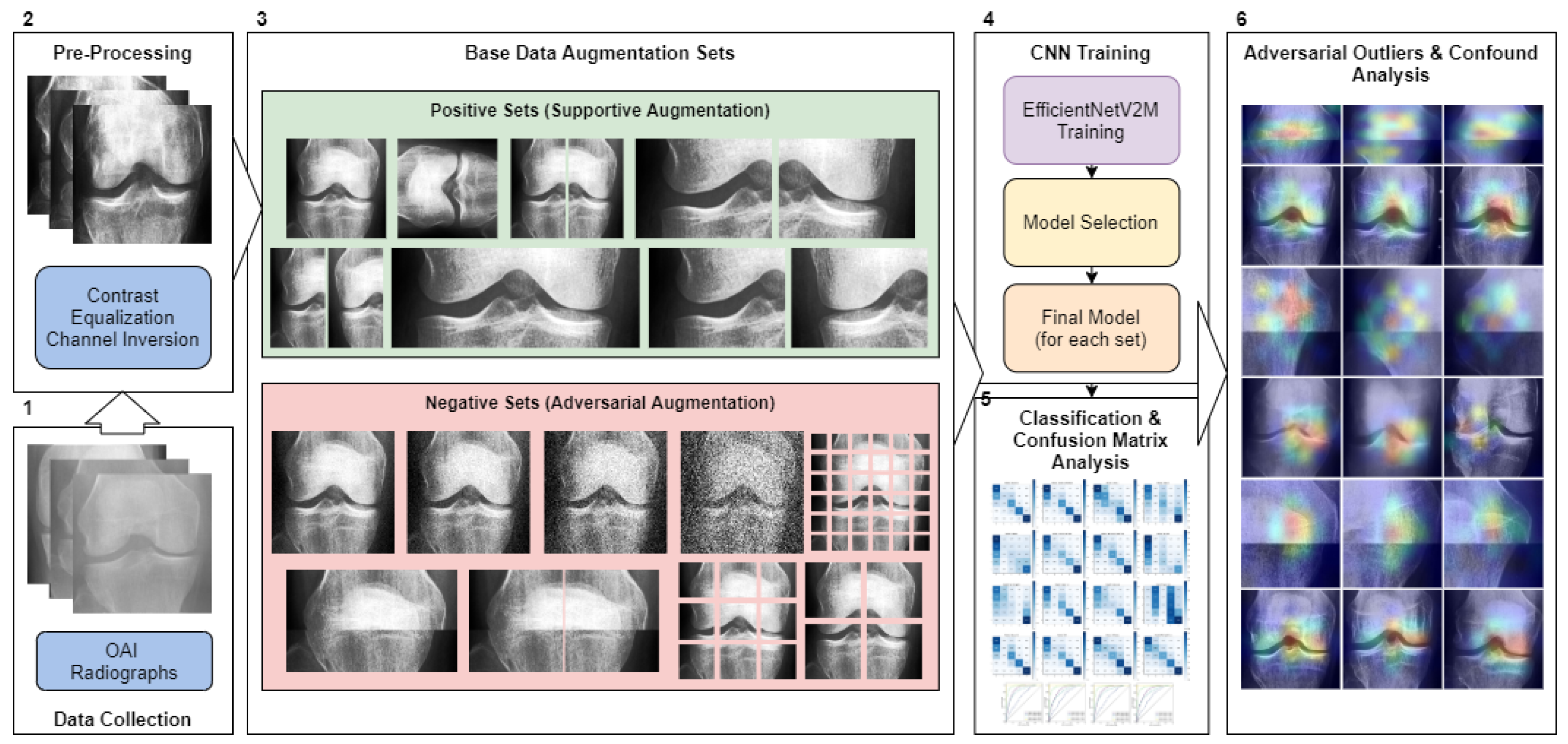Figure 1 illustrates the study’s operational sequence using numeric markers. This section elaborates on each step in the order indicated by the numeric markers in the figure.

2.1. Data Collection

Our research utilized knee joint X-ray images from the Chen 2019 study [49], originally sourced from the Osteoarthritis Initiative (OAI) [45]. The OAI, a multi-center study focused on biomarkers for knee osteoarthritis, and included 4796 participants aged 45 to 79. We employed the pre-processed primary cohort data from Chen 2019 [49], which had undergone automatic knee joint detection, bounding, and zoom standardization to 0.14 mm/pixel. 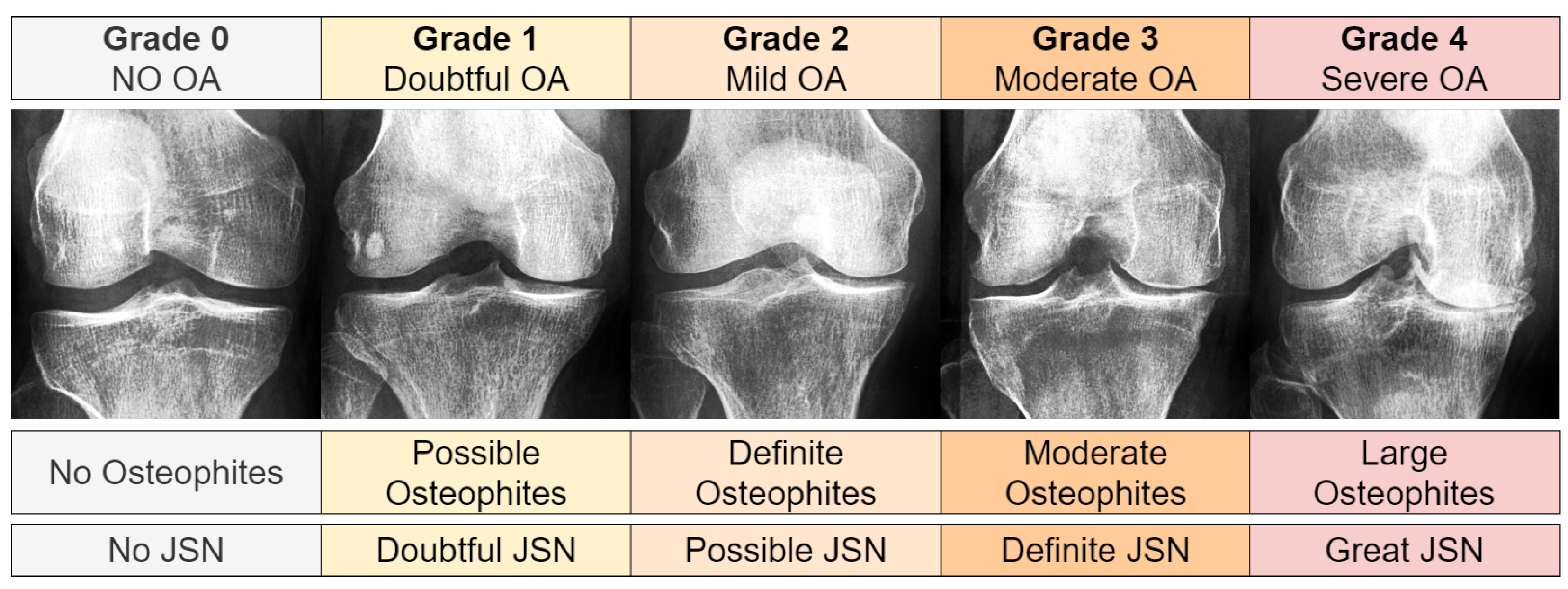This process yielded 8260 images ($224\times 224$ pixels) derived from 4130 X-rays, each containing both knee joints. The images were graded using the Kellgren and Lawrence (KL) system [46], as shown in Figure 2. The KL grade distribution was as follows: 3253 images for Grade 0, 1495 for Grade 1, 2175 for Grade 2, 1086 for Grade 3, and 251 for Grade 4.

2.2. Image Pre-Processing

We flipped each right knee joint image to mirror a left knee orientation. Then, we identified and inverted any negative channel images, resulting in 189 such alterations for KL01 and 77 for KL234. We then equalized the image histograms’ contrast using Equation (1). In this equation, for a given grayscale image $\mathit{I}$ with dimensions of $m\times n$, we used the cumulative distribution function (cdf) and pixel value v to obtain an equalized value $h\left(v\right)$ in the range $[0,255]$. Here, ${\mathrm{cdf}}_{\min }$ represents a non-zero minimum value of the image’s cumulative distribution, while $m\times n$ signifies the total number of pixels.

$$h\left(v\right)=255\frac{\mathrm{cdf}\left(v\right)-{\mathrm{cdf}}_{\min }}{\left(mn\right)-{\mathrm{cdf}}_{\min }}$$

(1)

2.3. Base Data Augmentation Sets

In our research, we divided our dataset into distinct splits and applied base data augmentations to each of these splits. We created two sets of base data augmentations. The term ‘base data’ refers to permanent modifications made to all the data (‘offline’) before introducing any ‘online’ affine augmentations during the training phase (

Table 1. Online (affine) augmentation approaches, occurring randomly during training.

Augmentation Method	Description	Training Configuration
Image Rotation	Implements a counter-clockwise rotation on images	Allows a rotation of up to 40 degrees
Width Shifting	Moves the image laterally along the x-axis	Allows a shift of up to 45 pixels along the x-axis
Height Shifting	Moves the image vertically along the y-axis	Allows a shift up to 45 pixels along the y-axis
Shearing	Distorts the image along the width or height axis	Implements a maximum shear angle of 0.2 degrees
Zooming	Modifies the image scale, zooming in or out within the frame	Enables a maximum of 20% zoom
Horizontal Flipping	Creates a mirror image along the vertical axis	Implements flipping only along the horizontal axis

). The first set of augmentations focused on positive or supportive modifications, exploring the potential benefits of incorporating image-based artificial diversity during training. The second set, conversely, involved negative/adversarial augmentations, intended to challenge the classifier. This approach aimed to help identify potential confounds in the classification task and test the model’s resilience.

Table 2. Offline-additive base data augmentation sets, citations indicate the first known KOA instance of the approach.

Base Augmentation	Type	Description
Baseline	Positive	Original image without any changes
Baseline Rotated	Positive	Original image rotated counter-clockwise
ROI [39]	Positive	Image segmented to highlight the Region of Interest
Horizontal Split 20%	Positive	Image horizontally split in the middle with a 20% overlap
Horizontal Split 20% Flip	Positive	Image horizontally split in the middle with a 20% overlap, and the second part flipped
Horizontal Split	Positive	Image horizontally split in the middle with a 5% overlap
Horizontal Split Flip	Positive	Image horizontally split in the middle with a 5% overlap, and the second part flipped
ROI Split [31]	Positive	ROI segmented image split in the middle with a 20% overlap
ROI Split Flip	Positive	ROI segmented image split in the middle with a 20% overlap, and the second part flipped
Noise 05	Negative	5% Gaussian pixel noise added to the baseline
Noise 10	Negative	10% Gaussian pixel noise added to the baseline
Noise 20	Negative	20% Gaussian pixel noise added to the baseline
Noise 50	Negative	50% Gaussian pixel noise added to the baseline
Cube 2	Negative	Image divided into equidistant parts in a $2\times 2$ grid
Cube 3 [40]	Negative	Image divided into equidistant parts in a $3\times 3$ grid
Cube 6	Negative	Image divided into equidistant parts in a $6\times 6$ grid
No ROI	Negative	Concatenated upper and lower non-ROI parts of the image
No ROI Split	Negative	Concatenated upper and lower non-ROI parts of the image, split in the center

showcases all the conditions used, while Figure 3 visualizes the base augmentations made. The specifics of each type of augmentation are further elaborated in the following section.

2.4. Affine (Online) Augmentation

Affine augmentations typically involve geometric transformations, such as scaling, translation, rotation, and shearing, applied in real-time during model training. These online augmentations introduce a diverse range of geometric variations to training images, essential for enhancing model generalization. By exposing the model to different orientations and scales, affine transformations help to improve pattern recognition robustness to such variations, a critical aspect in tasks like image classification and object detection. These transforms are typical for almost every RGB-based image classification task.

2.5. Offline Base Data Augmentations

Offline base data augmentations involve pre-applied, static modifications to the entire dataset before training commences. These augmentations, ranging from simple image alterations to complex transformations, are crucial for introducing initial diversity to the training set (before online augmentation). They play a significant role in expanding the dataset’s variability, particularly beneficial in limited or less diverse datasets, and aid in reducing overfitting and enhancing the model’s performance.

2.5.1. Positive/Supportive Data Augmentations

Positive augmentations, a subset of offline base data augmentations, involve modifications that supportively enhance the dataset. These include variations of the original images and mild transformations that maintain the data’s core characteristics. Such augmentations are vital for enriching the dataset with beneficial variability, aiding in more nuanced feature extraction and understanding of data variations, ultimately leading to improved model accuracy and reliability.

2.5.2. Adversarial/Negative Augmentations

Adversarial augmentations are crucial in assessing model performance under challenging conditions. By introducing substantial alterations such as noise and complex distortions to the dataset, these augmentations provide insights into the model’s sensitivity and robustness. They are instrumental in revealing how the model’s performance degrades in difficult circumstances, highlighting its limitations and areas for improvement. Additionally, adversarial augmentations help in identifying confounds within images, clarifying which aspects of the data the model might erroneously rely on. This process is vital for ensuring that the model’s predictive capabilities are not only based on genuine features relevant to the task but are also resilient to misleading or irrelevant data variations.

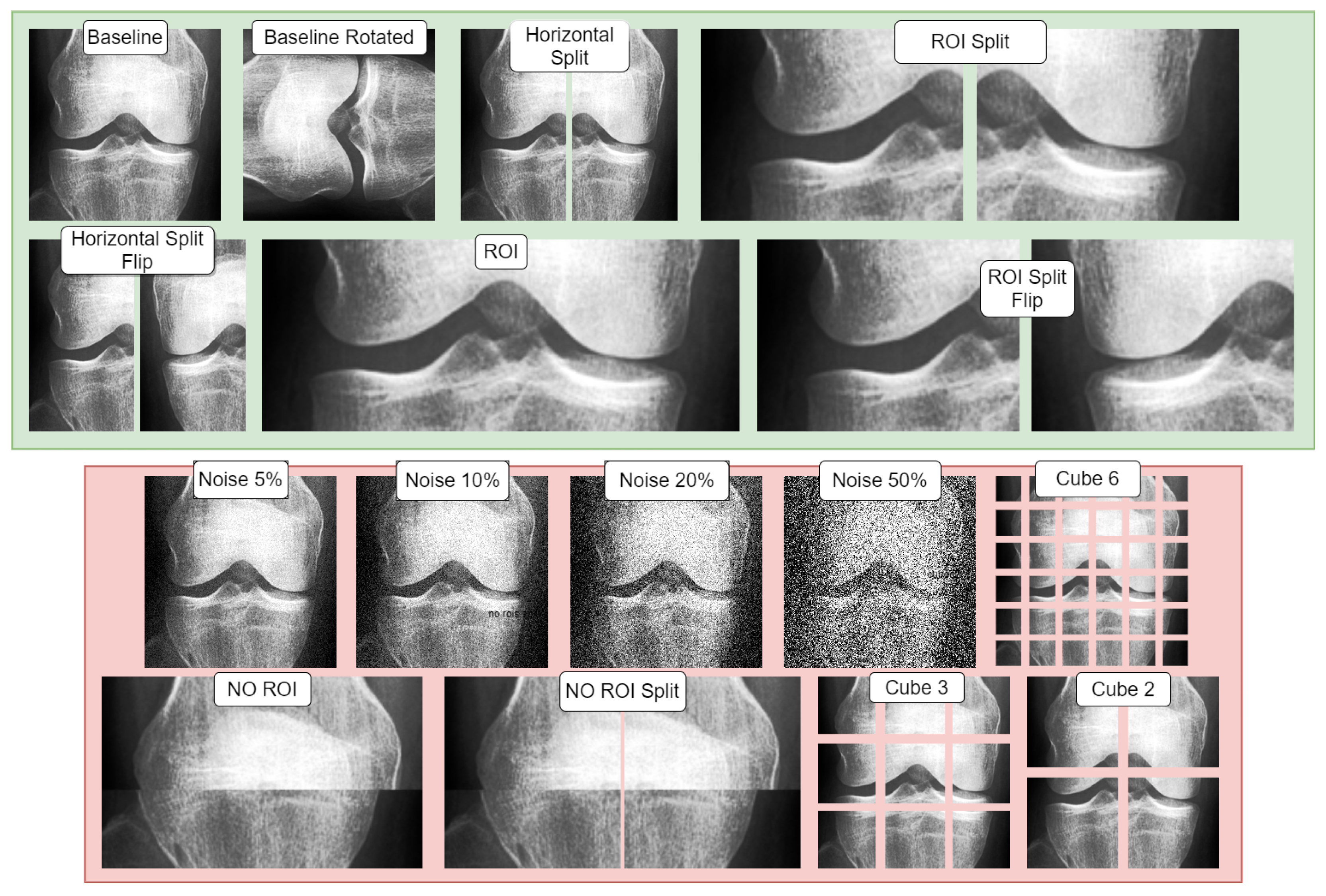
2.5.3. Adversarial (Negative) and Supportive (Positive) Augmentations Visualization

Figure 3 illustrates both adversarial and supportive/positive augmentations. In the green window, the supportive augmentations are displayed as variants of the provided baseline image. Likewise, in the red window, one can observe the adversarial variants and their visual form, all applied on the same unaltered baseline image shown in the green window.

2.6. Convolutional Neural Networks

Convolutional neural networks (CNNs) [50] are foundational in the recent deep learning revolution [3]. CNNs are a type of neural network often used for computer vision. These neural networks employ the convolution operation between input and a filter-kernel. Filters slide across inputs to highlight features in a response known as a feature map. Various feature maps are combined to produce higher-level feature maps corresponding to higher-level concepts. Formally [51], for an image $\mathit{I}$ of $u\times v$ dimensions and filter-kernel $\mathit{H}$ of $s\times t$ dimensions, we can obtain feature map $\mathit{G}$ by convolution across the two axes with kernel $\mathit{H}$ as:

$$\mathit{G}(u,v)=\sum _s\sum _t\mathit{I}(u,v)\mathit{H}(u-s,v-t)$$

(2)

Typically, the feature map values are filtered with an activation function. The role of the activation function is to re-map the values across a given function.

2.7. Convolutional Neural Network Architecture

The EfficientNet architecture, as introduced by Tan and Le in their 2019 paper [52], stands as a significant milestone in the evolution of deep learning architectures. It is based on the principle of compound scaling, a novel approach that meticulously balances three fundamental dimensions of a neural network: depth, width, and resolution. Depth refers to the number of layers in the network, width to the size of each layer, and resolution to the size of the input image that the network processes. This balance is crucial, as it allows EfficientNet to scale up in a more structured and efficient manner compared to previous architectures.

The scaling process itself can be underpinned formaly in Equation (3):

$$d={\alpha }^{\varphi }{d}_0,w={\beta }^{\varphi }{w}_0,r={\gamma }^{\varphi }{r}_0$$

(3)

In this formula, $\alpha ,\beta ,$ and $\gamma$ are constants that determine how each dimension scales, while $\varphi$ is a user-defined coefficient that dictates the overall scaling of the model. The base values $d_0,w_0,r_0$ represent the depth, width, and resolution of the base model, respectively. This formulation allows for a systematic and controlled scaling of the network dimensions, leading to improvements in model performance.

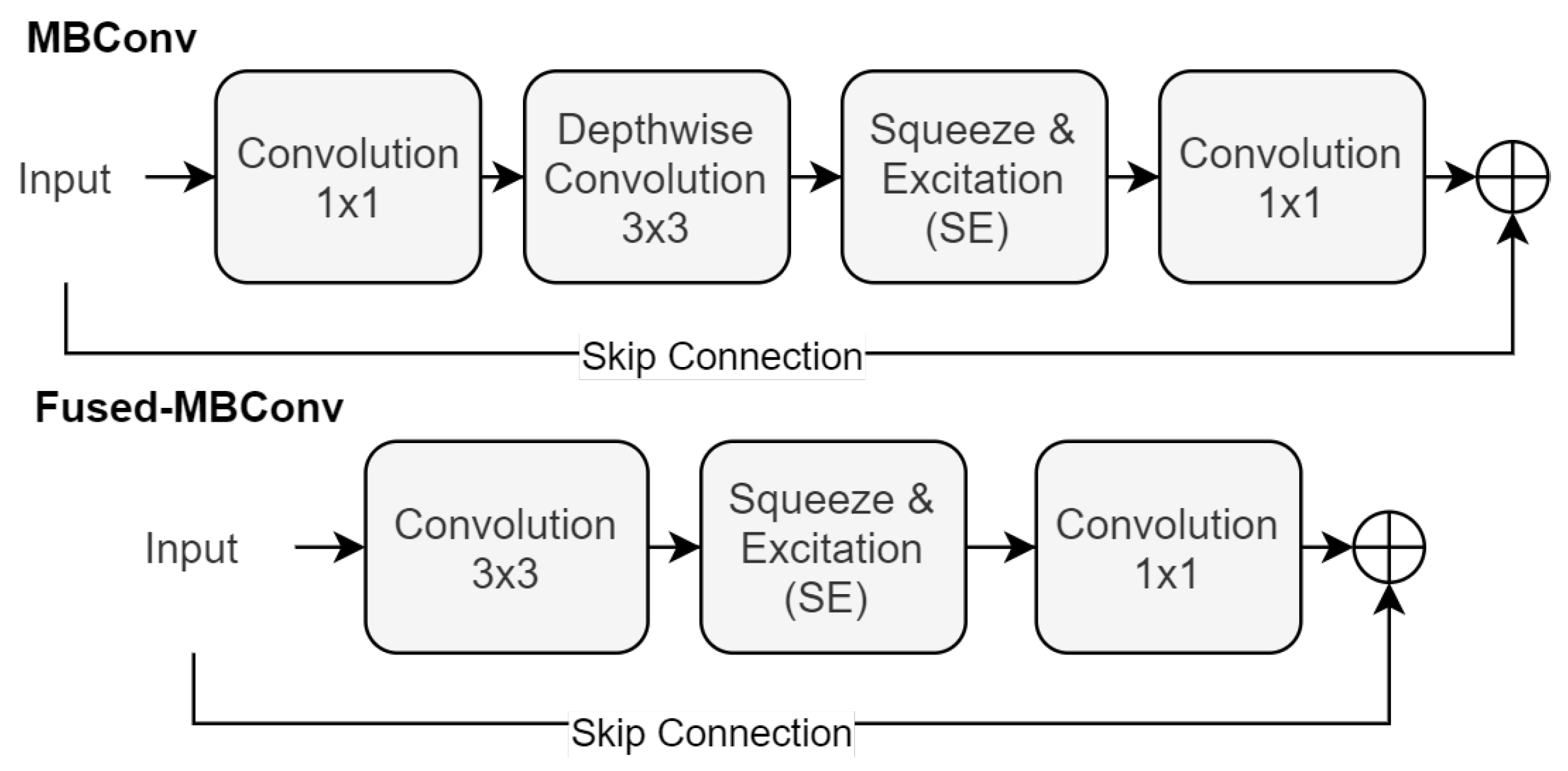
At the heart of EfficientNet’s design is the MBConv block, a series of transformations that are crucial for its effectiveness. This block sequences a $1\times 1$ convolution, a depth-wise convolution, a Squeeze-and-Excitation (SE) operation [53], and concludes with another $1\times 1$ convolution, as shown in Equation (4):

$$T_{MB}\left(\mathit{I}\right)={\mathit{K}}_2\ast SE(\mathit{D}\ast ({\mathit{K}}_1\ast \mathit{I}))$$

(4)

Here, ${\mathit{K}}_1$ and ${\mathit{K}}_2$ represent the $1\times 1$ convolutional filters, $\mathit{D}$ is the depth-wise convolutional filter, and $\mathrm{SE}$ denotes the Squeeze-and-Excitation operation. This arrangement of operations is pivotal in enhancing the network’s ability to focus on the most informative features of the input.

Building upon the foundations laid by EfficientNet, the EfficientNetV2 [47] introduces an evolution in the form of the Fused-MBConv block. This new block design streamlines the architecture by combining the initial $1\times 1$ and depth-wise convolutions into a single $3\times 3$ convolution. This is then followed by an SE operation and a final $1\times 1$ convolution, as detailed in Equation (5):

$$T_{FMB}\left(\mathit{I}\right)={\mathit{K}}_2\ast \left(SE({\mathit{K}}_f\ast \mathit{I})\right)$$

(5)

In this configuration, ${\mathit{K}}_f$ refers to the $3\times 3$ convolutional filter that merges the initial $1\times 1$ and depth-wise convolutions. ${\mathit{K}}_2$ represents the final $1\times 1$ convolutional filter. Each convolution in this sequence is followed by an activation function, and the architecture may include skip connections to facilitate effective training and convergence. Figure 4 showcases both the MBConv and Fused-MBConv Block.

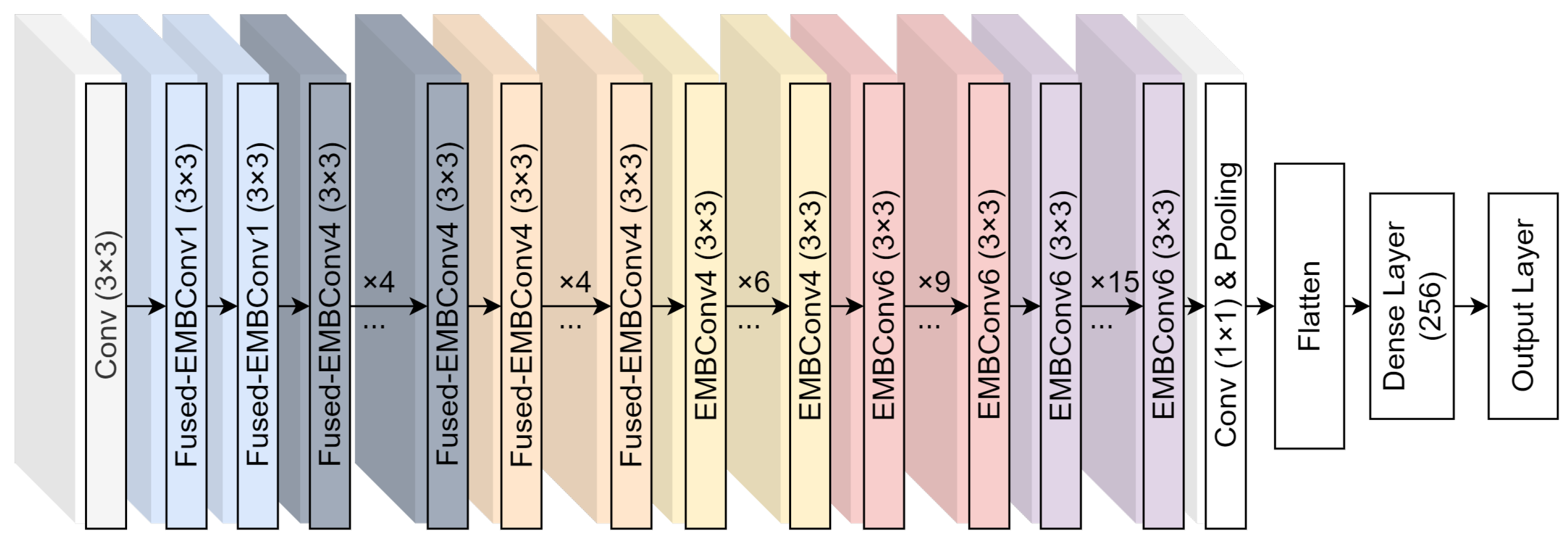
Figure 5 provides a visual representation of the base EfficientNetV2 model (B0) and the modifications we have implemented. These modifications are aimed at enhancing the network’s performance in specific applications, demonstrating the adaptability and scalability of the EfficientNet architecture.

Our study employed EfficientNetV2-M, enhancing it with flattening and 256-neuron dense layers. The training process was executed over 15 epochs using the Adam optimizer [54], with the dataset divided into Training (75%), Validation (15%), and Testing (15%) sets (patient aware splits). The minimum validation loss determined early stopping. All CNN training and online affine augmentations were implemented with the open-source library Deep Fast Vision [55]. All offline affine augmentations are consistently applied to each image, but the degree to which they are applied is randomized within the specified ranges of each technique. These augmentations are directly incorporated and executed using the Keras library [56].

We chose the EfficientNetV2-M for our study due to its high performance on ImageNet [57] and it’s maximal compatibility with our NVIDIA Tesla P100 GPU, which allowed us to fully leverage its computational capabilities. This choice was further supported by EfficientNet’s efficient training times and its advanced architecture enabled us to achieve competitive scores while efficiently utilizing our entire computational resources. The experiments were carried out on the computation servers at the University of Jyväskylä in Finland.

2.8. CNN Interpretability

While the complexity of neural networks increases their capabilities, it also complicates the interpretation of their predictions. Due to this complexity, these systems are often considered ‘black boxes’. However, the Grad-CAM [48] algorithm, based on the CAM [58] framework, helps reduce this ‘black box’ effect. At a high level, Grad-CAM is an algorithm that visualizes how a convolutional neural network makes its decisions. It creates what are known as “heat maps” or “activation maps” that highlight the areas in an input image that the model considers important for making its prediction. The Grad-CAM spatial activation map $M_{Grad-CAM}^p$ can be calculated using the $\mathrm{ReLU}$ activation function on the sum of neuron importance weights $b_k^p$ multiplied by feature maps ${\Psi }^k$ as shown below:

$$M_{Grad-CAM}^p=\mathrm{ReLU}\left(\sum _{k}b{k}^p{\Psi }^k\right),\mathrm{where}b{k}^p=\frac{1}{Z}\sum _m\sum _n\frac{\partial y^p}{\partial {\Psi }_{mn}^k}$$

(6)

In this equation, $b_k^p$ are the neuron importance weights of feature map k for class p, $\frac{\partial y^p}{\partial {\Psi }_{mn}^k}$ represents the partial derivative of the final layer prediction for class p ($y^p$) with respect to the last convolutional layer’s kth feature map ${\Psi }_{mn}^k$. Z is the total pixels, and $m,n$ are the indexes for each element within feature map k. ${\Psi }^k$ is the feature map k given by the last convolutional layer, spatially averaged. In our study, we extracted Grad-CAM activations from the layer immediately preceding the flattening operation.

2.9. Figures of Merit

In evaluating the results of our experiment, we employ several key figures of merit to quantify the performance.

Accuracy is the proportion of true results (both true positives and true negatives) among the total number of cases examined. It can be calculated using the following equation:

$$\mathrm{Accuracy}=\frac{\mathrm{TP}+\mathrm{TN}}{\mathrm{TP}+\mathrm{TN}+\mathrm{FP}+\mathrm{FN}}$$

(7)

Precision (also called positive predictive value) is the fraction of relevant instances among the retrieved instances. It is calculated as follows:

$$\mathrm{Precision}=\frac{\mathrm{TP}}{\mathrm{TP}+\mathrm{FP}}$$

(8)

Recall (also known as sensitivity, hit rate, or true positive rate) is the fraction of the total amount of relevant instances that were actually retrieved. The equation for recall is:

$$\mathrm{Recall}=\frac{\mathrm{TP}}{\mathrm{TP}+\mathrm{FN}}$$

(9)

The F1 score is the harmonic mean of precision and recall. It aims to find the balance between precision and recall. The F1 score can be calculated as follows:

$$\mathrm{F}1=2\frac{\mathrm{Precision}\mathrm{Recall}}{\mathrm{Precision}+\mathrm{Recall}}$$

(10)

In these formulas, TP stands for True Positives, TN for True Negatives, FP for False Positives, and FN for False Negatives.

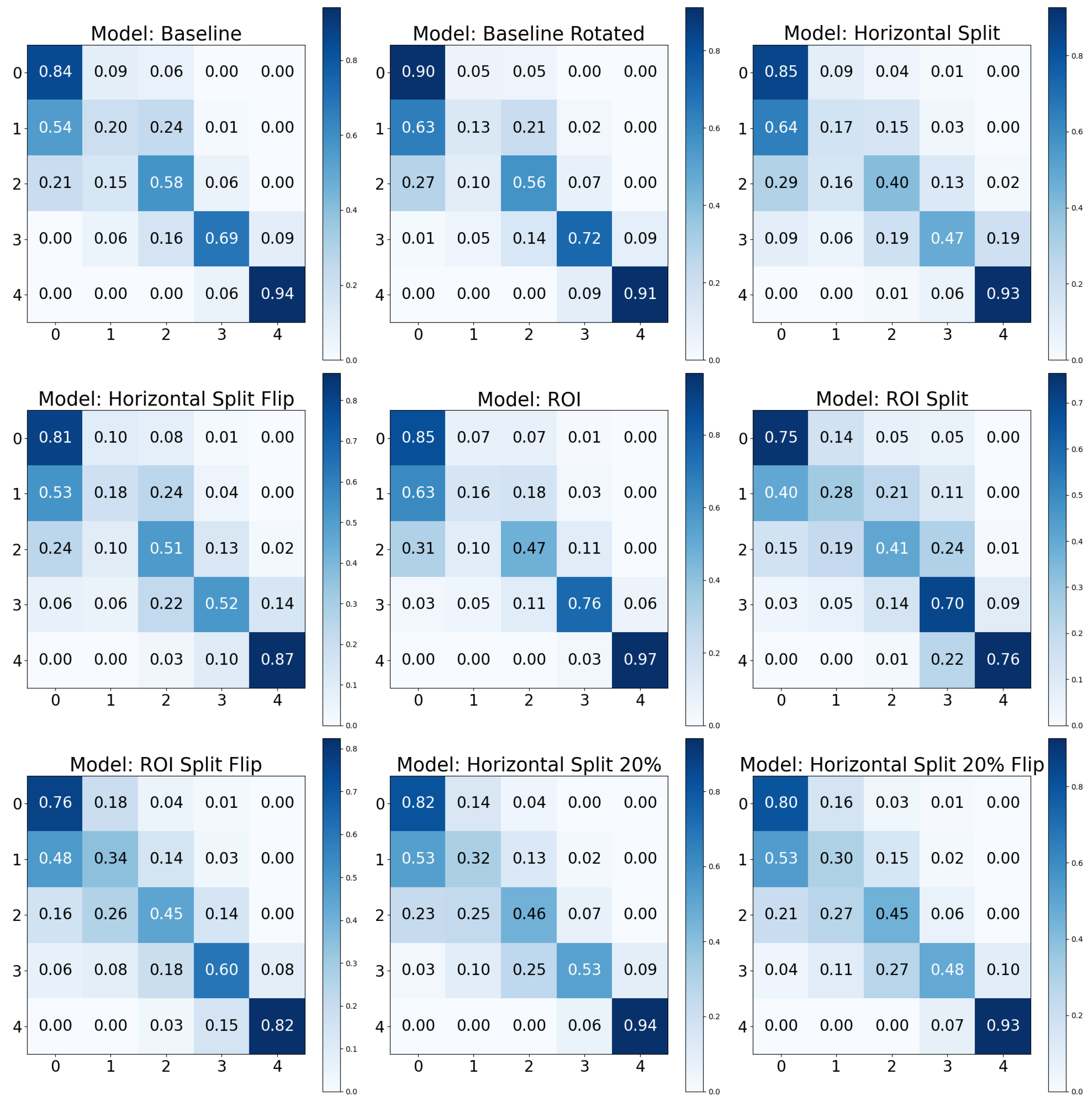
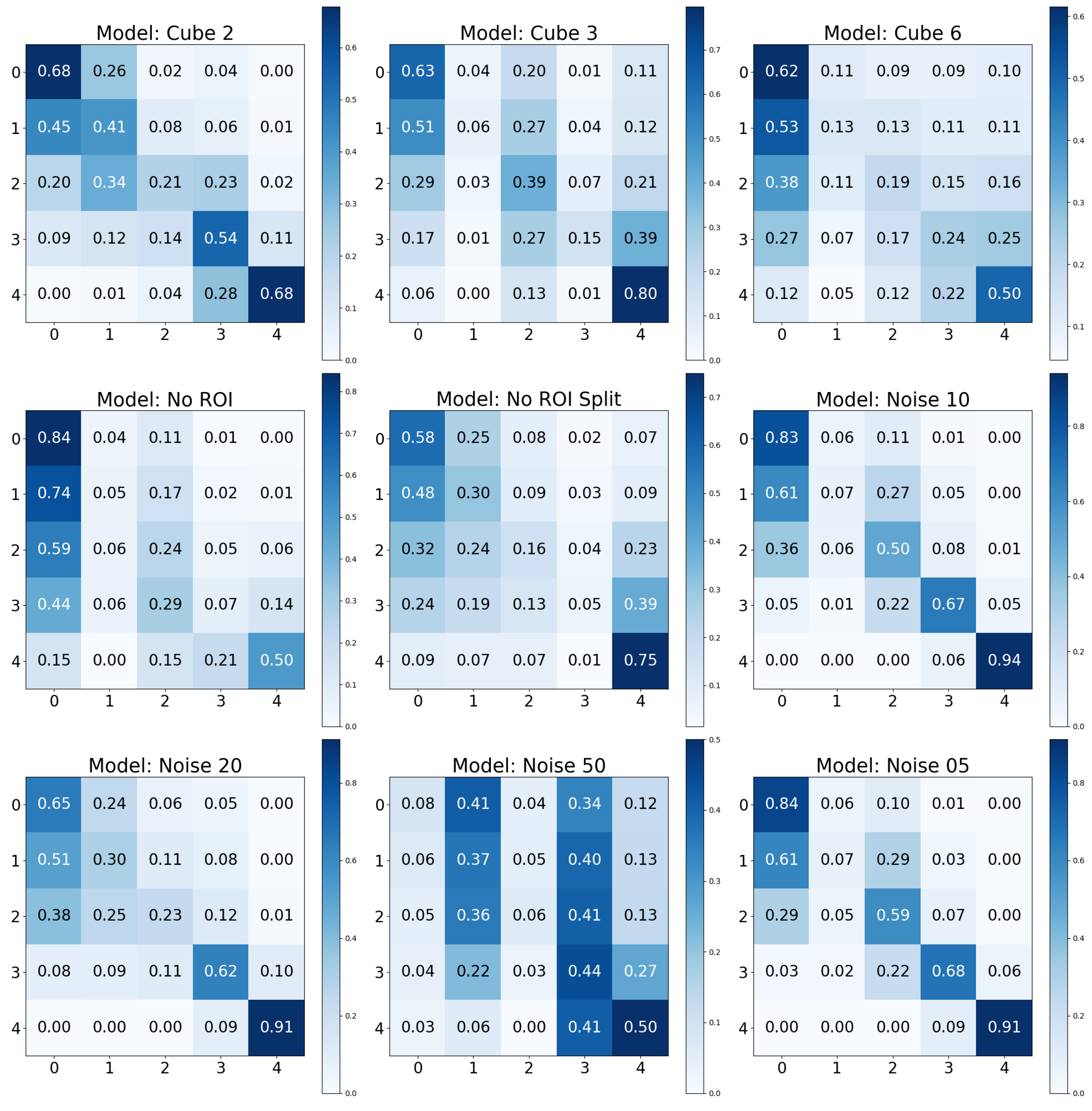
2.10. Confusion Matrix

To further elucidate the model’s performance, especially in a multi-class setting, the confusion matrix is an essential tool. A confusion matrix is a tabular representation that allows for the visualization of a model’s performance. Each row of the matrix represents the instances in an actual class, while each column represents the instances in a predicted class. The diagonal cells represent the number of correct classifications for each class, while the off-diagonal cells indicate errors.

The confusion matrix not only provides a clear visual of the performance but also showcases the calculation of various performance metrics, including recall for each class (normalized matrix diagonal). This is particularly important in multi-class classification problems, where understanding the model’s performance for each class is critical. While accuracy gives a general overview of the model’s performance, recall provides essential insight into the model’s ability to correctly identify each class. This is crucial in scenarios where certain classes are more significant or have greater consequences associated with misclassification.

In our study, we normalized the confusion matrices for each class so that the sum of values in each row equals 1. This normalization ensures that the diagonal elements of the matrix represent the recall for each class. By adopting this approach, the matrix not only indicates how well the model classifies each category but also allows for a direct and clear comparison of class-specific performance. The row-wise normalization simplifies the understanding of the matrix, making it more intuitive to evaluate the recall, as the values directly reflect the proportion of correctly identified instances for each class.

3. Results

3.1. Positive Augmentations

In

Table 3. Performance metrics of the model on the test set using positive/supportive base augmentations.

Model Name	Accuracy	Precision	Recall	F1-Score
Baseline Rotated	0.655	0.621	0.645	0.618
Baseline	0.644	0.621	0.651	0.627
ROI	0.623	0.614	0.643	0.616
Horizontal Split 20%	0.595	0.597	0.611	0.591
Horizontal Split Flip	0.581	0.518	0.577	0.531
ROI Split Flip	0.583	0.577	0.595	0.579
Horizontal Split 20% Flip	0.577	0.578	0.591	0.570
ROI Split	0.570	0.533	0.579	0.546
Horizontal Split	0.560	0.497	0.563	0.501

, the model with the best performance appeared to be the “Baseline Rotated” model, obtaining an accuracy of 0.655, Precision of 0.621, Recall of 0.645, and an F1-Score of 0.618 (The names of the models represent various augmentation approaches, indicating that the base data was transformed in accordance with the methods outlined in Table 2. The results presented correspond to the performance of these models when evaluated on the test set after the training process.). The high accuracy indicated that this model was successful in correctly predicting the classification most of the time, while the substantial F1-Score, which is a harmonic mean of precision and recall, indicated a balanced high performance in both these areas. This suggested that the model could retrieve a high proportion of relevant instances (high recall), while ensuring the proportion of instances it claimed to be relevant were indeed relevant (high precision).

In contrast, the model with the lowest performance in the evaluation was the “Horizontal Split” model. With an Accuracy of 0.560, Precision of 0.497, Recall of 0.563, and an F1-Score of 0.501, this model consistently fell behind the other models across all performance metrics, indicating lower overall performance. It can be observed that there was a clear downward trend in performance metrics from the “Baseline Rotated” model to the “Horizontal Split” model. Interestingly, models using the “Flip” modification, such as “Horizontal Split Flip” and “ROI Split Flip”, tended to have a lower performance than their non-flip counterparts. The only exception to this was the “Horizontal Split 20% Flip” model, which slightly outperformed the “ROI Split” and “Horizontal Split” models, suggesting that the impact of the “Flip” modification could be influenced by broader image overalp (0.20 in that case).

The provided confusion matrices in Figure 6 revealed the performance of nine distinct models: Baseline, Baseline Rotated, Horizontal Split, Horizontal Split Flip, ROI, ROI Split, ROI Split Flip, Horizontal Split 20%, and Horizontal Split 20% Flip. The Baseline model performed well for KL0 and KL4 but encountered difficulties with the intermediate classes. This issue was partly alleviated in the Baseline Rotated model for KL0. The Horizontal Split and Flip models demonstrated variability in performance across classes, with the Flip version slightly improving the accuracy for KL2 and KL3. The Region of Interest (ROI) models exhibited improvements for the intermediate classes, especially KL2. The ROI Split and Flip models offered a more balanced performance across classes, particularly for KL0 and KL1. Lastly, the Horizontal Split 20% and its Flip variant showed high misclassification rates between KL0 and KL1, although the Flip version brought some improvement. However, KL4 was well classified across all models, suggesting distinct features that differentiated it from other classes. Models with the “Flip” modification seemed to have a more evenly distributed confusion matrix, indicating a more balanced prediction across different classes. However, this did not always result in overall higher performance, as seen in the “Horizontal Split Flip” model. The ”Baseline Rotated” model seemed to perform well for the first and last class, but its performance decreased notably for the other classes. This behavior was shared across models, where models often performed better for the first and last class. The ”ROI” and “ROI Split” models presented a similar pattern, with typical performance in the first and last classes.

Reviewing the results from the different model iterations, it was quite unexpected to find that the ROI (Region of Interest) models did not manage to outperform the Baseline models. Given that the Baseline models leveraged the entire image and the ROI models focused on the specific region expected to contain more relevant information for the task, it was anticipated that the ROI models would perform better. Figure 7 showcases ROC curves for the ROI model against the baseline.

Upon evaluation of AUCs in the one-vs-all scheme (Figure 7), it was observed that Classes 0, 2, and 3 had marginally higher AUC scores in the Baseline Model compared to the ROI Model. Specifically, the AUC for Class 0 was 0.87 in the Baseline Model versus 0.85 in the ROI Model, suggesting that the Baseline Model was slightly more successful in distinguishing between positive and negative instances for this class. Similarly, for Class 2, the Baseline Model had an AUC of 0.84 compared to 0.81 in the ROI Model, and for Class 3, the AUC was 0.96 in the Baseline Model versus 0.95 in the ROI Model. In contrast, for Class 1, the ROI Model outperformed the Baseline Model, albeit slightly, with an AUC of 0.69 against 0.68. For Class 4, both models performed impeccably, achieving a perfect AUC score of 1.00, demonstrating their ability to distinguish instances of this class perfectly.

In summary, while the performance of both models was similar for all classes, the Baseline Model showed a slight edge in Classes 0, 2, and 3. The ROI Model only performed marginally better in Class 1, and both models were equally successful in Class 4. Despite these differences in AUC values, it’s noted that the curvature along the axis was similar between the two models. This suggestsed that the trade-off between sensitivity and specificity (true positive rate and false positive rate) was similar for both models across different decision thresholds. This similarity in shape indicated that both models had similar performance trade-offs, even if the absolute performance (as measured by AUC) varied slightly.

3.2. Negative (Adversarial) Augmentations

In

Table 4. Performance metrics of the model on the test set using negative/adversarial base augmentations.

Model Name	Accuracy	Precision	Recall	F1-Score
Noise 05	0.619	0.592	0.616	0.591
Noise 10	0.591	0.572	0.601	0.574
Noise 20	0.478	0.489	0.544	0.495
Cube 2	0.483	0.469	0.502	0.458
No ROI	0.427	0.315	0.343	0.289
Cube 3	0.407	0.347	0.406	0.299
Cube 6	0.359	0.287	0.333	0.272
No ROI Split	0.349	0.294	0.371	0.263
Noise 50	0.186	0.262	0.291	0.174

, we find a comparison of several adversarial augmentation models based on metrics including Accuracy, Precision, Recall, and F1-Score. The model with noise level 05 had the highest performance across all metrics. As noise increased (i.e., Noise 10 and Noise 20), a corresponding decrease was observed in all performance metrics. This suggested that lower levels of noise improved the model’s ability to generalize. In comparison, higher noise levels degraded the performance, likely due to interference with essential radiograph features. The models using cube techniques also showed varying levels of performance. Cube 2, for instance, performed better than Cube 3 and Cube 6 in all aspects. This could imply a potential optimal size or representation for the cube that best captured critical information. The models with no Region of Interest (ROI) performed poorly compared to others. The Noise 50 model recorded the lowest performance.

In Figure 8, the Cube 3 model performed well when identifying KL0; however, as the Kellgren-Lawrence (KL) grades increased, this performance gradually diminished, culminating in a notable difficulty when classifying KL4. This suggested that while the model could easily distinguish KL0 from other classes, the higher grades posed more of a challenge. In contrast, the Cube 2 model showed a more even performance across all KL grades, with a gradual decrease in accuracy from KL0 to KL4. While the model also performed best on KL0 and worst on KL4, it demonstrated a more balanced confusion across different classes. The Cube 6 model continued the trend observed in Cube 3 and Cube 2, struggling with higher KL grades and decreasing performance from KL0 to KL4. Interestingly, it confused KL0 with KL1 and KL3 more than Cube 3 and Cube 2, which indicated its difficulty differentiating between these classes.

Shifting to the Noise models, Noise 10 and Noise 05 displayed interesting behavior. They were fairly accurate when classifying the extreme KL grades (KL0 and KL4), but encountered difficulties with the intermediate classes. The Noise 20 model, like Cube 2, demonstrated an evenly distributed performance across the grades, but it performed slightly better on class KL4 than Cube 2. This could point to a better ability to differentiate between the features of the KL4 grade. The Noise 50 model was unique in its performance, showing a high confusion rate, particularly between KL0 and KL1, and KL1 and KL3. It also struggled with KL0, KL1, and KL2, yet performed reasonably well on KL4, indicating that this model found the lower and intermediate KL grades more challenging.

Lastly, the No ROI model showed exceptional performance when classifying KL0, but it struggled to differentiate KL0 from KL2, and performed notably poorly on KL3. Similarly, the No ROI Split model showed a distinct performance pattern. It was particularly adept at identifying KL0 and KL4.

In the No ROI model, the high score for the KL0 class (0.84) indicated that the model effectively identified patterns associated with KL0. However, there is an absence of the primary region of interest. Similarly, the No ROI Split model achieved a surprisingly high score of 0.75 for the KL4 class. This suggested that these models were identifying other image features unrelated to the knee joint to make the classification decisions for these particular grades.

Figure 9 illustrates the Receiver Operating Characteristic (ROC) curves for both the “No ROI” and the “No ROI split” configurations. Notably, the model’s performance appeared virtually indistinguishable across these settings when employing a one-versus-all scheme. However, we must also pay attention to the markedly high Area Under Curve (AUC) values for KL 0 (>0.70) and KL 4 (>0.88). These elevated values, alongside the accompanying confusion matrices, underscored the prevalence of potential confounding regions within these images. Remarkably, these potential confounding regions enabled a level of classification precision that is both significant and surprising, particularly given the absence of a region of interest, such as the entire knee joint. We further investigated these outlier results in the next section.

3.3. Adversarial Outliers

In this section, we expand on our results corresponding to the identified outlier classifications–specifically, “No ROI” and “No ROI Split”. To deepen the analysis and provide clearer insights, we compare these outcomes with the baseline results, enabling a more comprehensive comparative evaluation.

In Figure 10, we noticed identical scores from the ‘Baseline’ and ‘No ROI’ models for KL0. This observation suggests either that the absence of a large region of interest (ROI) does not affect KL0 classification or that true class region confounds are visible. Additionally, the ‘No ROI Split’ model demonstrated performance remarkably similar to the ‘Baseline’ model for KL4. Although it did not achieve complete alignment with the ‘Baseline’, its relative success hinted at similar influences as observed in KL0. Most notably, we observed a clear performance boost for KL1 in the ‘No ROI Split’ model. This class is historically the most challenging for classification in Knee-Osteoarthritis. Remarkably, this score was the highest individual KL1 score across all examined models in this study.

To delve deeper into these paradoxical results, we applied the Grad-CAM technique to the top examples from each of the previously mentioned classes. As shown in Figure 11, in the first row (No ROI KL0), we observed activations focused on texture and potential outlines of the patella. On the other hand, the second row (Baseline KL0) displayed control images that distinctly highlighted the knee joint. However, it is essential to note the broad spread of activation extending across and above the knee joint. Observations in the third row (No ROI Split KL4) revealed unclear patterns, primarily centered around what seemed to be a focus on wear-related texture. Despite the ambiguity, the controls (row 4) highlighted the knee joint, albeit with significantly less spread than the KL0 control (second row). Examining the KL1 focus in the first image of the last set (fourth row) revealed what appeared to be a part of the patella outline. In contrast, the other two images (fourth row) depicted a non-specific texture focus. Finally, all controls (KL0, KL4, KL1) presented a wide activation range that extended slightly over the knee joint. Overall, our observations suggested that the baseline models for KL0 tended to rely not only on the knee joint but also incorporated broader areas for their classifications. This starkly contrasted with the KL1 baseline models, which seemed to concentrate more on the knee joint.

4. Discussion

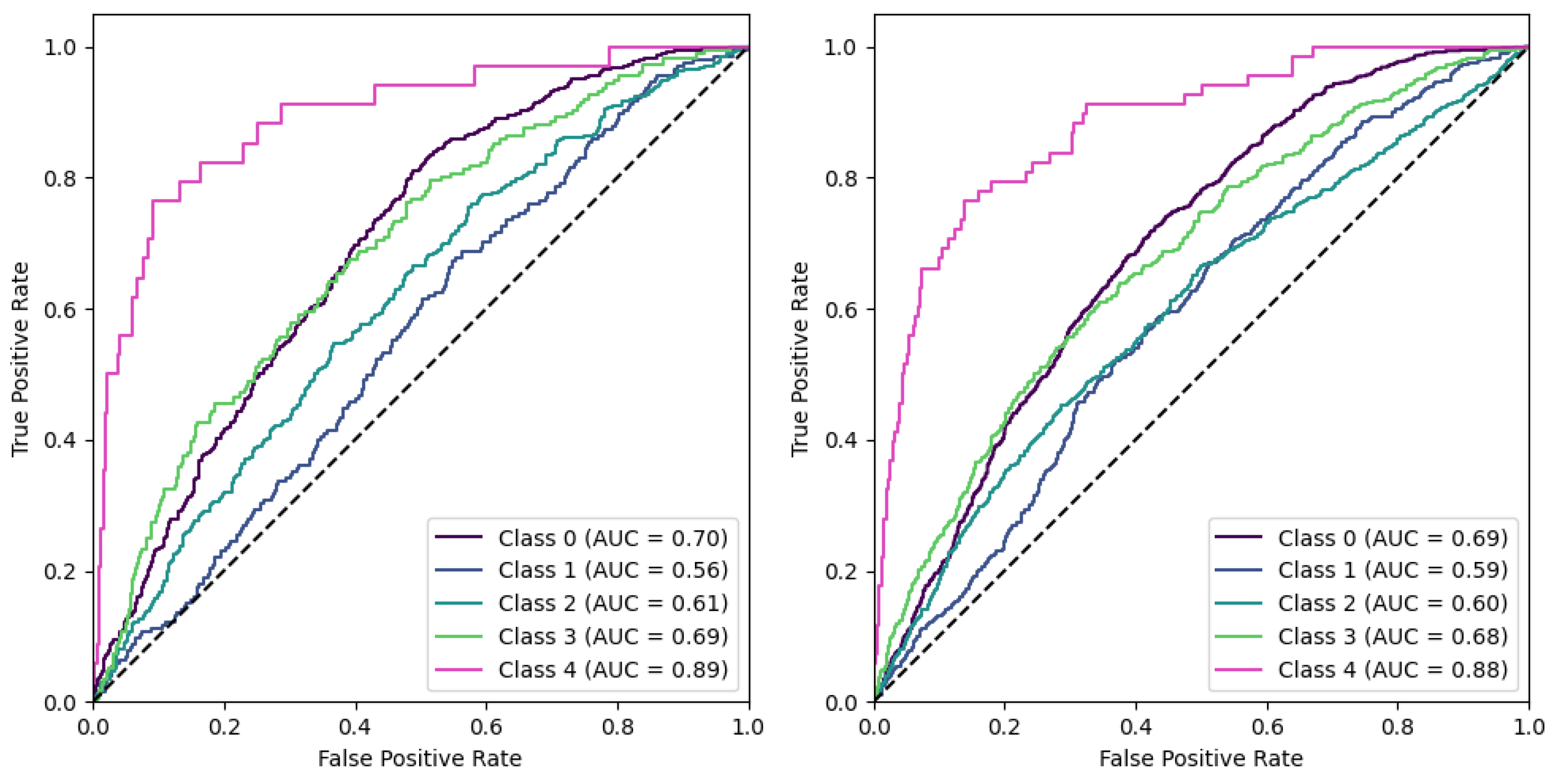
Our analysis has highlighted the marked effectiveness of certain positive data augmentations in improving model performance. Specifically, the ‘Baseline Rotated’ model showed the highest accuracy but second-best recall. Incorporating rotation into our baseline model could have increased its robustness to orientation changes in the images, contributing to its superior accuracy. Furthermore, the confusion matrix analysis demonstrated excellent recall for the KL0 and KL4 grades, a result that may be associated with the distinct radiographic features of these classes. Conversely, the ‘Horizontal Split’ model, which divided the image into two parts along the horizontal axis, performed the worst across all considered metrics. This could be because this approach might eliminate or distort crucial radiographic features, thereby reducing the model’s ability to classify the images accurately. Notably, the results contradicted our initial expectation that the ROI models would outperform the baseline models, given the assumption that focusing on specific regions containing more relevant information would increase performance. However, the results indicated that models utilizing the entire image data might have a slight edge in performance over those focusing on a particular ROI, suggesting that potentially important information outside the ROI might be missed, or that confounds are integrated, inflating the performance.

Furthermore, when evaluating performance, the recall metric offered an additional layer of insight. For instance, despite a slight drop in accuracy, the ‘Baseline’ model showed a higher recall than the ‘Baseline Rotated’ model, underscoring its capability to comprehensively identify relevant cases. This can be a critical consideration in fields like medical diagnostics, where certain classes might have greater consequences associated with misclassification. This observation revealed that when dealing with significantly skewed class distributions, utilizing the baseline modality may lead to more evenly distributed performance across the relevant classes.

While data augmentation techniques have been widely adopted in deep learning, studies specifically investigating their effects in the medical imaging domain remain sparse. Often, the choice of augmentation techniques relies heavily on informal recommendations or generic best practices that aren’t always tailored to the unique challenges and characteristics of medical images [37]. This lack of systematic exploration can lead to suboptimal model performance or even introduce biases. In this context, the studies by Goceri [37] and Hussain et al. [38] stand out as notable exceptions that delve into the intricacies of various additive augmentation methods and their impact on model performance in medical imaging tasks.

The study by Goceri [37], spanning different medical imaging domains such as lung CT, mammography, and brain MR images, observed distinct patterns in the effectiveness of additive augmentation. For lung CT images, translating and shearing produced the highest accuracy of 0.857, whereas mere translation yielded the lowest at 0.610. In mammography images, the combination of translation, shearing, and clockwise rotation was most effective, achieving an accuracy of 0.833, while adding ‘salt-and-pepper’ noise and shearing underperformed, achieving only 0.667. For brain MR images, the same combination of translation, shearing, and clockwise rotation outperformed other methods with an accuracy of 0.882, while adding ‘salt-and-pepper’ noise and shearing showed the lowest accuracy at 0.624. Another investigation by Hussain et al. [38] explored different mammography additive augmentation techniques, producing varied results. Notably, the Shear augmentation achieved the highest training accuracy of 0.891 and a validation accuracy of 0.879. Conversely, Noise augmentation was the least effective, with training and validation accuracies of 0.625 and 0.660, respectively. Augmentations such as Gaussian Filter, Rotate, and Scale also demonstrated high accuracy in training and validation phases. Comparing our results, those of Goceri, and the findings from Hussain et al., it becomes evident that while some augmentation methods consistently show effectiveness across studies, their efficacy can vary based on domain specificity and dataset nuances. Our results, especially those pertaining to the ‘Baseline Rotated’ model, suggest that certain augmentations, such as rotation, might have unique advantages in the context of KOA.

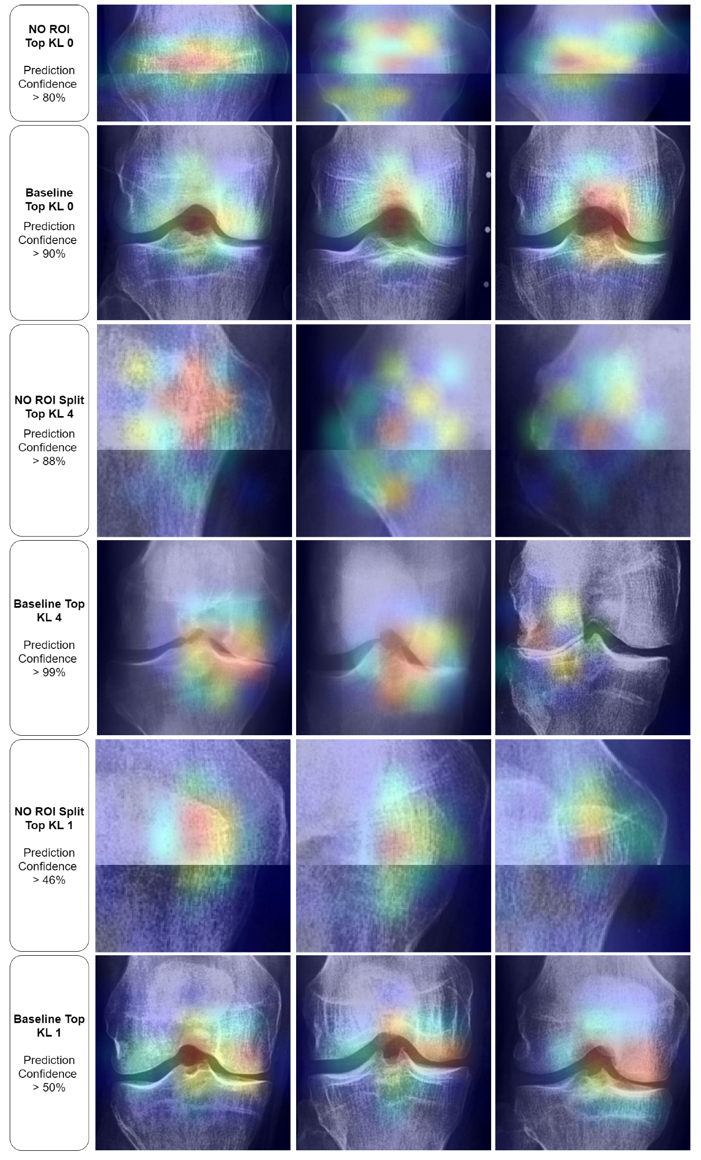
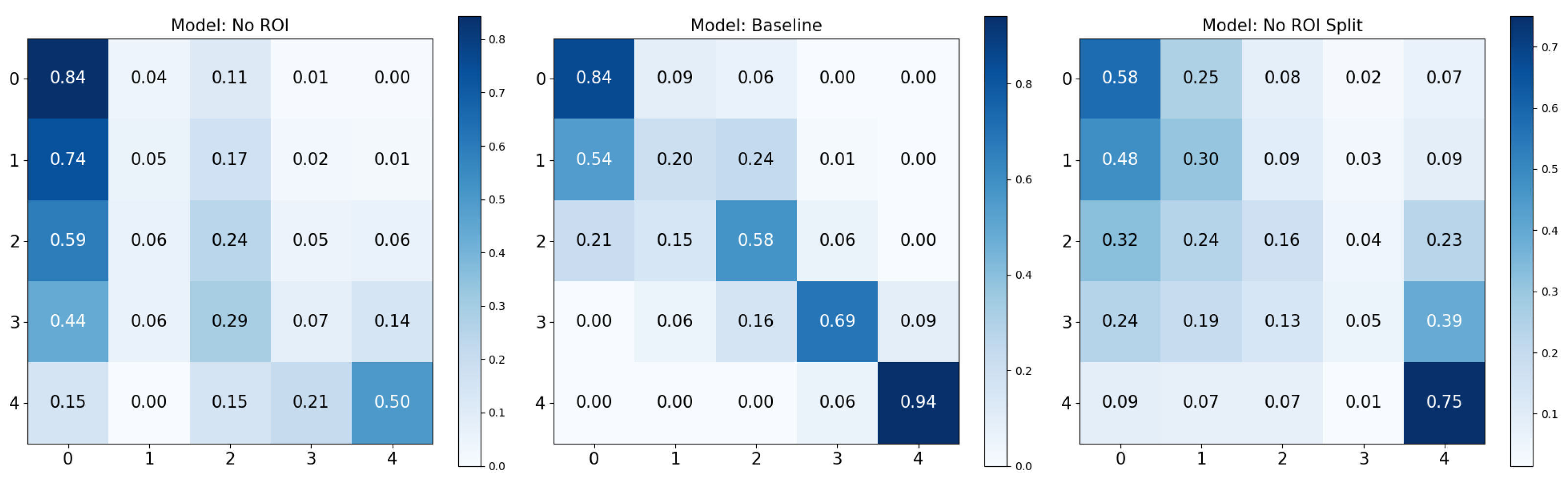
Adversarial (negative) augmentations, in the form of adversarial attacks, were explored in our study. It was observed that as the noise level increased, the models’ performance deteriorated, suggesting that the introduction of excessive noise could disrupt the discernment of relevant features within the images. Interestingly, the models lacking a Region of Interest (ROI) performed poorly overall. However, these models did exhibit exceptionally high performance for specific KL grades, such as KL0 and KL4, which may indicate the presence of confounding variables that the model leverages to make its predictions. The results for the “No ROI” and “No ROI Split” models were particularly intriguing. Despite the absence of a region of interest, the high-performance scores achieved by these models for specific KL grades suggest that they might be identifying other image features unrelated directly to knee joint osteoarthritis for classification decisions. In the case of KL0, the identical scores from the ‘Baseline’ and ‘No ROI’ models suggest either that the absence of an ROI may not affect KL0 classification or that true class confounds are visible. For KL4, the ‘No ROI Split’ model demonstrated performance remarkably similar to the ‘Baseline’ model, hinting at similar influences. The most notable result, however, was the clear performance boost for KL1 in the ‘No ROI Split’ model. This class is historically challenging to classify in Knee-Osteoarthritis studies, making this finding particularly interesting.

Regarding adversarial attacks and augmentation within the broad spectrum of medical domain literature, we identify three main categories. The first category encompasses studies focused on adversarial attacks with a specific objective [41,42,43,44] (e.g., to alter the prediction for a single instance or a set of instances towards a target or model behaviour). The second category involves adversarial augmentation without an explicit optimization pipeline (e.g., noise injection) dedicated to a clearly defined adversarial objective [37]. This category primarily includes adversarial augmentations. It appears that the distinction lies in the experimental approach; adversarial augmentation studies are exploratory, seeking to detect issues through analysis, in contrast to the first category, where the aim is to induce a specific issue or effect. The third category includes research that examines specific known or hypothesized biases, such as hospital identification bias [59], and thus the experimental design is constructed towards investigating the bias. To our knowledge, our method of cropping based adversarial augmentation, which unveiled potential confounds upon analysis, is novel. This is especially pertinent as adversarial augmentations in the medical field predominantly focused on noise injection. To the best of our knowledge, and throughout our review, we found no similar studies that identified potential confounds in medical images by eliminating regions of interest.

In our study, the primary goal was to evaluate base data augmentation within a naturalistic paradigm, where the use of affine augmentations is applied consistently across all datasets. This approach mirrors standard practices in neural network learning scenarios. By including affine augmentations in every set, we ensure a level playing field, allowing for an accurate comparison with the baseline set whose base data remained unmodified. This methodology is crucial because omitting affine augmentations from certain sets while only augmenting the base data could skew results. Affine approaches have consistently demonstrated effectiveness in enhancing model performance and mitigating overfitting. Therefore, to avoid giving an unfair advantage to these approaches, our study incorporates them uniformly across all datasets. This strategy ensures that our primary comparison point—the baseline set without base data modifications—remains a reliable standard for evaluating the effectiveness of base data augmentation within this naturalistic paradigm.

In the “No ROI” image, the upper portion of the patella is visible, along with the upper femur and the medial and lateral femoral condyles. The lower portions of the tibia and fibula are also evident. However, the entire medial and lateral tibial plateaus are missing. The Grad-CAM visualizations for these “No ROI” images show activations concentrated on peripheral regions of the knee joint, such as the edges of the femur and tibia that do not articulate directly. Consequently, the omission of the tibial plateaus means that the critical weight-bearing surfaces of the knee joint, essential for assessing osteoarthritis, are absent from the image. The joint space, crucial for evaluating the degree of cartilage loss and joint space narrowing, cannot be visualized either. The absence of the articulating surfaces largely prevents the assessment of osteophyte presence, subchondral bone sclerosis, and cyst formation, all key features used to grade the severity of osteoarthritis according to the Kellgren and Lawrence grading system.

Further insights from our Grad-CAM visualization analysis indicate potential confounding regions that might affect our models’ decision-making processes. Notably, in the absence of a designated region of interest (ROI) for KL0, the models tend to focus on the texture and contours of the patella. Interestingly, this pattern shifts with the baseline KL0 models, where the joint and its eminence are distinctly highlighted. However, the spread of activation that extends broadly across and above the knee joint suggests the model might be considering features beyond the knee joint for classification. In the No ROI Split KL4, the model appeared to be using general wear-and-tear texture indications for their classifications, which may not be directly related to disease progression but rather to the participant’s age. Finally, in the KL1 category, the models oscillate between specific and non-specific textures, further underscoring potential confounding regions.

Regarding Grad-CAM limitations, it is important to highlight that Grad-CAM has several limitations that can lead to misinterpretations. Firstly, it often highlights correlations rather than causations, meaning the regions it emphasizes may not be causally linked to the prediction. It is also limited to convolutional layers, providing no insight into how other types of layers contribute to the model’s decision. Grad-CAM can fail to localize multiple instances of the same class, and for single class examples, it may fail to localize the entire region of the class [60]. Users might over-rely on these visual explanations for model validation, potentially overlooking other issues like biases in training data. Furthermore, Grad-CAM may also fall short in capturing complex, abstract reasoning that isn’t spatially localized. Its effectiveness is tied to model architectures, and different architectures may yield varying results, limiting generalizability. Additionally, if a model is overfitted, Grad-CAM might highlight non-generalizable, idiosyncratic features. Lastly, it often misses the global context of the image, focusing only on local features, which may not always convey the complete picture necessary for accurate interpretation. These limitations underscore the importance of using Grad-CAM cautiously and in conjunction with other validation methods to ensure a comprehensive understanding of model behavior.

Incorporating findings from Saporta et al. [61], the application of saliency methods like Grad-CAM in medical imaging appears to demand scrutiny, particularly in their role in diagnostic decision-making. The authors conducted a comprehensive evaluation of seven saliency methods, including Grad-CAM, across diverse neural network architectures. A notable aspect of their study was the establishment of the first human benchmark for chest X-ray segmentation in a multilabel classification context. The study’s results indicated that while Grad-CAM was generally more effective than its counterparts in highlighting pathologies, all the evaluated saliency methods were more prone to fail in localizing important pathologies compared to human experts. This gap in performance was particularly evident in cases of pathologies that were smaller and had more complex shapes. Additionally, the research highlighted a positive correlation between the confidence level of the model and the accuracy of Grad-CAM in localizing pathologies. These findings emphasize the need for caution and further research before considering the integration of saliency methods like Grad-CAM into real-world clinical settings.

From our results, one high-performing set involved rotation, which may be partly attributed to the rotated orientation of the knee joint along the vertical axis of the radiograph image. In this configuration, the convolution operation repeatedly encounters relevant features as it slides across the image, potentially leading to more condensed and effective feature maps. This is in contrast to a non-rotated radiograph image, where the knee joint occupies only a single vertical segment of the image. In this latter case, the convolution would likely traverse the entire joint just once or twice, depending on the receptive field, making feature extraction potentially slightly less effective. However, we previously discussed how the ‘baseline’ configuration enhanced recall values, which is a significant factor, especially in scenarios where missing true positives is costly. By utilizing the baseline modality, we may achieve a more evenly distributed performance across the relevant classes, ensuring that the system is not only accurate but also consistently reliable in identifying true instances across different categories.

Integrating adversarial augmentations into the study of various diseases offers considerable advantages. For instance, selectively omitting regions of interest (ROIs)—whether through dynamic clustering algorithms or predetermined for specific diseases—might reveal potential confounds, especially if the model’s key performance indicators remain stable despite these alterations. Adding pixel noise is another strategic augmentation that serves two critical functions: it underscores potential disruptions in the classification process and uncovers specific sensitivities of the employed architecture to noise. This insight is particularly valuable; for example, if a solution demonstrates extreme sensitivity to noise, it could inform the decision to incorporate affine blurring transformations during the training phase to mitigate this issue. Such strategies not only bolster the robustness of the models but also deepen our understanding of disease detection and classification, thereby enhancing the precision and reliability of medical imaging analyses.

In assessing the underperformance of certain methods, particularly the horizontal split approach, it becomes apparent that this technique may inherently dilute the informativeness of the image data. In knee radiography, pathological changes are often more pronounced on one side of the knee joint. When the image is split horizontally, one half may carry less informative features but is still labeled similarly to the more informative half. This dilution of label information could be a significant factor contributing to the reduced efficacy of this method. The horizontal split essentially divides the image into two halves that may not equally contribute to the accurate classification of the knee joint’s condition, leading to a skewed or incomplete understanding of the disease’s manifestation.

Furthermore, the underperformance of the Region of Interest (ROI) model can be contrastively elucidated by examining why the ‘No ROI’ model performed exceptionally well for the extreme classes. It has been recognized that patient age correlates with the progression and stage of osteoarthritis (OA). Interestingly, neural networks might still infer age-related information even when the knee joint is absent from the image. Indicators such as faint signs of sclerosis and the general condition of the remaining knee radiograph may inadvertently provide age-related clues. This is particularly relevant in the later stages of OA, where osteophytes can be exceptionally large and located further from the knee joint. Consequently, we suspect that age may be a confounding variable that the models are inadvertently leveraging. Such a hypothesis warrants further investigation that would help to explain both the ‘ROI’ underperformance and the ‘No ROI’ overperformance at the extremes.

To further investigate this hypothesis, future studies should consider directly targeting age as a classification (or regression) variable. Utilizing the ROI, Baseline, and Non-ROI model sets in this context could provide valuable insights into the extent to which age can be predicted from knee radiographs. Such an approach would not only help in understanding the potential confounding influence of age on OA automatic grading but also contribute to the broader discourse on the interpretability and reliability of neural network decisions in KOA medical imaging. This exploration into the intersection of age, disease markers, and AI model performance might be crucial for refining automatic tools and ensuring that they are as accurate and unbiased as possible. This setup, focusing on the relationship between age and OA manifestations in knee radiography and its impact on AI models, warrants further investigation and could potentially lead to more nuanced and accurate classification methods in the future. In this endeavor, we also consider the participation of medical experts mandatory for validation purposes, and broader discussions on the clinical implications of the outcomes.

Our findings regarding pixel noise underscore an essential consideration in raw radiograph data, which may contain parts of suboptimal quality with substantial pixel noise. These observations align with similar findings reported in other studies [37,38].The classifier sensitivity to noise was particularly acute in the no-OA to early grade classes (KL0-1), where even a minimal noise level of $5\%$, led to a decline in early grade performance. This decline in early grade performance might be explained by the point that noise may falsely trigger or mask faint osteophyte features or other similar features in the images which are characteristic of early stages OA, leading to misinterpretations by the deep learning model during training. Moreover, a critical issue in digitized X-rays is the severe aliasing problems that may occur. Aliasing can introduce what is known as aliasing-associated noise. Such noise may interfere by creating misleading artifacts. Overall noise artifacts raise questions about the inclusion of low-quality radiographs in classification systems. They also underscore the necessity for research aimed at establishing guidelines for acceptable levels of noise, including aliasing-associated noise. One possible intervention could involve incorporating blur effects in the image augmentation process. However, it’s important to note that the effectiveness of this method specifically addresses pixel noise, and its impact on aliasing issues remains unclear. On the other hand, the effect of aliasing and methods to mitigate it on the performance of these systems is an area that is not yet well understood and requires further investigation. We could consider that severe noise artifacts and aliasing might even interfere with medical expert analysis, as well as artificial neural networks. In pursuing this endeavor, we deem the involvement of medical professionals essential for validation purposes and for engaging in more extensive discussions about the clinical implications.

Further studies are needed to confirm the presence, and by extension the extent of confounding factors in non-adversarial images. If such factors might exist in non-adversarial contexts this is of particular concern. This could lead in systems augmented with non-adversarial images, where models could misinterpret non-disease related features, potentially leading to overdiagnosis or misdiagnosis if used as computer-assisted diagnostic aids. Clinicians must understand the reasoning behind a model’s decision to trust and use it effectively. Models that focus on non-specific features could result in decisions that are counterintuitive or misaligned with clinical knowledge. Therefore, models should undergo rigorous validation and evaluation before deployment. This process should involve not only statistical metrics but also feedback from medical professionals, ensuring that the model’s decision-making process aligns with clinical expertise.

5. Conclusions

In this study, we evaluated the effectiveness of various base data augmentation techniques to enhance model performance in knee-joint osteoarthritis classification. These findings have potential implications for future work in this area, particularly for improving the robustness, recall, and accuracy of deep-learning models in medical image analysis. However, our results also highlight the need to carefully consider potential confounding regions to ensure that the models primarily base their predictions on relevant features. To facilitate further analyses, we provide open access to all data, trained models, and an extensive set of the top 20 Grad-CAM images, ranked by prediction confidence.