A Self-Adaptive Meta-Heuristic Algorithm Based on Success Rate and Differential Evolution for Improving the Performance of Ridesharing Systems with a Discount Guarantee

Abstract

One of the most significant financial benefits of a shared mobility mode such as ridesharing is cost savings. For this reason, a lot of studies focus on the maximization of cost savings in shared mobility systems. Cost savings provide an incentive for riders to adopt ridesharing. However, if cost savings are not properly allocated to riders or the financial benefit of cost savings is not sufficient to attract riders to use a ridesharing mode, riders will not accept a ridesharing mode even if the overall cost savings is significant. In a recent study, the concept of discount-guaranteed ridesharing has been proposed to provide an incentive for riders to accept ridesharing services through ensuring a minimal discount for drivers and passengers. In this study, an algorithm is proposed to improve the performance of the discount-guaranteed ridesharing systems. Our approach combines a success rate-based self-adaptation scheme with an evolutionary computation approach. We propose a new self-adaptive metaheuristic algorithm based on success rate and differential evolution for the Discount-Guaranteed Ridesharing Problem (DGRP). We illustrate effectiveness of the proposed algorithm by comparing the results obtained using our proposed algorithm with other competitive algorithms developed for this problem. Preliminary results indicate that the proposed algorithm outperforms other competitive algorithms in terms of performance and convergence rate. The results of this study are consistent with the empirical experience that two people working together are more likely to come to a correct decision than they would if working alone.

1. Introduction

Shared mobility is a paradigm of transport modes that enables the reduction of vehicles, traffic congestion, consumption of energy and emission of greenhouse gas in cities. Due to the potential benefits of shared mobility, different sharing models have emerged in the past years. These include ridesharing, car sharing and bike sharing. As all of these transport models are helpful for sustainability issues, relevant issues and problems have attracted researchers’ and practitioners’ attention in academia and industry. In particular, ridesharing has been implemented in university campuses [1], by companies [2] and by transport service providers such as Uber [3], Lyft [4] and BlaBlaCar [5].

In the literature, early studies of ridesharing focused on the problem of meeting the transport requirements of drivers and passengers. A lot of the work from the early ridesharing literature can be found in [6,7]. In these early works, the goal was to optimize total cost savings or total travel distance through matching drivers and passengers based on their itineraries. The ways to achieve this goal can include building a simulation environment to simulate the application scenarios or formulating an optimization model to solve the ridesharing problems. Due to the wide variety of ridesharing problems, different models were proposed and studied in the past years. Optimization methods were applied to formulate the ridesharing problems. The challenges and opportunities for solving ridesharing problems with optimization models can be found in [8,9]. A review on variants of shared mobility, problems and solution approaches is available in [10].

In addition to the issues of optimizing total cost savings or total travel distance [11], there are recent works on other issues in ridesharing systems. For example, to promote ridesharing, the optimization of monetary issues and non-monetary issues in ridesharing systems has been studied. As mentioned in [12,13,14], dealing with these issues often requires the modeling of more complex constraints that are highly nonlinear. These constraints may lead to a more complex solution space and make it difficult to find a solution for the problem. Therefore, these monetary issues and non-monetary issues in ridesharing systems pose new challenges in the development of effective methods to solve relevant ridesharing problems.

One prominent financial benefit of a shared mobility mode such as ridesharing is cost savings. For this reason, a lot of studies focus on maximization of cost savings in shared mobility systems. Cost savings provide an incentive for riders to adopt ridesharing. However, if cost savings are not properly allocated to riders or the financial benefit of cost savings is not sufficient to attract riders to use ridesharing mode, riders will not accept ridesharing mode even if the overall cost savings is significant [15,16]. In a recent study [13], the concept of discount-guaranteed ridesharing has been proposed to provide an incentive for riders to accept ridesharing services through ensuring a minimal discount for drivers and passengers. In [13], several algorithms have been applied to solve the Discount-Guaranteed Ridesharing Problem (DGRP). With the advances in computing technology, it is possible to develop a more effective algorithm to solve the problem. In this study, we will propose an algorithm to improve the performance of the discount-guaranteed ridesharing systems and the convergence rate to find a solution for the DGRP. Neighborhood search has been recognized as an effective mechanism to improve solutions in an evolutionary computation approach. The concept of self-adaptation has been widely used in meta-heuristic algorithms to identify better search strategies through learning and to apply them in the solution-finding processes to improve convergence rate. In this paper, a success rate-based self-adaptation mechanism and neighborhood search are used jointly to develop an effective algorithm to solve the DGRP.

One of the challenges in solving the DGRP arises from the large number of constraints and discrete decision variables. To tackle the constraints effectively, we adopt a method that discriminates feasible regions from infeasible regions in the solution space [17] by designing a proper fitness function. To deal with the discrete decision variables, we use a transformation approach that transforms the real values of decision variables into discrete values. The contributions of this paper include the development of a new self-adaptive neighborhood search algorithm for solving the DGRP and the assessment of its effectiveness by comparing with existing methods.

The rest of this paper is organized as follows. In Section 2, we will provide a literature review of ridesharing problems and relevant solution methods. We will present the problem formulation and the model of the DGRP in Section 3. In Section 4, the details about the development of a solution algorithm based on self-adaptation and neighborhood search will be presented. In Section 5, the results obtained by applying the proposed algorithm and other competitive algorithms will be presented. We will discuss the results of experiments and conclude this study in Section 6.

2. Literature Review

In this section, we briefly review existing studies relevant to this paper. As we concentrate on the development of an effective algorithm for the DGRP based on success rate self-adaptation and neighborhood search, the papers reviewed in this section include two categories: papers related to ridesharing literature and papers relevant to self-adaptation and neighborhood search in an evolutionary computation approach. Papers related to ridesharing will be introduced first. Papers related to self-adaptation and neighborhood search in an evolutionary computation approach will be introduced next.

One of the sustainable development goals is to promote emerging paradigms to mitigate global warming by reducing the consumption of energies, greenhouse gas emissions and negative impact to the environment. With the global trend to achieve this goal, several transport modes such as ridesharing, car-sharing and bike-sharing have appeared in the transportation sector in the past two decades under the sharing economy. As one of the most important transport modes for shared mobility, ridesharing makes it possible for passengers and drivers with similar itineraries to share rides and enjoy cost savings. For a comprehensive survey of ridesharing literature, please refer to [6,7,18].

Although ridesharing is one of the transport modes with the most potential to achieve shared economy, there are still barriers and challenges for its acceptance by the general public. For example, the lack of trust in ridesharing is one factor that hinders users’ acceptance of ridesharing [14]. Several studies have been done on the barriers to the acceptance of ridesharing. The acceptance of ridesharing mode is influenced by several monetary factors and non-monetary factors. Monetary factors for the acceptance of ridesharing are directly related to the financial benefits due to cost savings [12]. Non-monetary factors are directly related to the safety and comfortability of ridesharing such as trust, enjoyability and social awareness. For example, the trust issue in ridesharing has been studied in [14]. In particular, providing a monetary incentive is essential for the acceptance of ridesharing. In this study, we propose a scheme to provide a monetary incentive for ridesharing participants.

As cost savings is recognized as one of the most prominent benefits from ridesharing, the objective of the ridesharing problem considered in most studies is to maximize overall cost savings or minimize the overall travel costs while meeting the transportation requirements of riders and drivers [11]. However, individual ridesharing participants may not enjoy the benefits of cost savings even if overall cost savings have been maximized or the overall travel costs have been minimized. To make individual ridesharing participants enjoy the benefits of cost savings, the overall cost savings must be allocated to individual ridesharing participants properly such that the benefit of cost savings is sufficient for ridesharing participants to accept ridesharing.

In [12], a problem formulation has been proposed to maximize the overall rewarding ratio. However, there is no guarantee that the minimal rewarding rate can be guaranteed even if the overall cost savings is maximized [13]. In [13], a problem formulation and associated solution methods are proposed to ensure that the rewarding rate can be guaranteed. However, scalability of the algorithms was not studied. In this study, we will propose a new algorithm for the DGRP formulated in [13] to improve the performance and convergence rate to guarantee satisfaction of the rewarding rate for ridesharing participants.

As the DGRP is a typical integer programming problem in which the decision variables are binary, the complexity of the problem grows exponentially with the problem size. Exact optimization approaches are computationally feasible only for small instances due to the exponential growth of the solution space as the instances grow. Therefore, approximate optimization approaches will be adopted to solve the decision problem. In the past decades, a lot of evolutionary algorithms were proposed to find solutions for complex optimization problems. These include the Genetic Algorithm [19], Particle Swarm Optimization algorithm [20], Firefly algorithm [21] and metaheuristic algorithms such as the Differential Evolution algorithm [22]. In the literature, a wide variety of variants in the Genetic Algorithm, Particle Swarm Optimization algorithm, Firefly algorithm and Differential Evolution algorithm can be found in [23,24,25,26], respectively. Although these approaches may be applied to find solutions for optimization problems, their performances vary. The studies of [27,28] show several advantages of the PSO approach over the Genetic Algorithm. The previous study of [29] indicates that the Differential Evolution approach performs better than the Genetic Algorithm. Evolutionary computation approaches such as PSO or DE algorithms are well-known metaheuristic algorithms. A metaheuristic algorithm refers to a higher-level procedure that generates or selects a heuristic to find a good solution to an optimization problem. In [30,31,32,33,34,35,36], several adaptive Differential Evolution algorithms have been proposed to solve optimization problems.

The goal of this study is to propose a more effective solution algorithm to improve the performance of the DGRP. In this study, we will combine a Differential Evolution approach with a success rate self-adaptation mechanism to develop a solution algorithm for the DGRP. The characteristics of the DGRP are different from the problems addressed in [30,31,32,33,34,35,36] as the decision variables of the DGRP are discrete whereas the decision variables of the problems studied in [30,31,32,33,34,35,36] are continuous real values. In this paper, the self-adaptation mechanism of [37] and the concept of the neighborhood search of [38] are applied jointly to develop an effective problem solver. Note that the self-adaptation mechanism of [37] and the neighborhood search concept of [38] are originally proposed for a continuous solution space. This study will verify effectiveness of combining the self-adaptation mechanism and neighborhood search mechanism for problems with a large number of constraints and discrete decision variables.

The problem addressed in this paper is the DGRP, which was formulated in [13]. This paper is different from the previous work [13] in that the proposed success rate-based self-adaptive metaheuristic algorithm is different from the ten algorithms proposed in [13]. The contribution of this paper is to propose a novel self-adaptive algorithm to improve the performance and convergence rate of discount-guaranteed ridesharing systems. We verified the effectiveness of the self-adaptive algorithm by conducting experiments. The results indicated that the proposed method improves the performance of the solution and convergence rate for finding the solution. Although the algorithm proposed in this paper is designed for the DGRP, it can be applied to other optimization problems. For example, the work reported in [14] also applied a similar approach to another instance of a trust-based ridesharing problem.

3. The Formulation of the DGRP

In this section, we will present the formulation of the DGRP based on a combinatorial double auction mechanism [39]. The variables, parameters and symbols used in this paper are listed in

Table 1. Notation of symbols, variables, and parameters.

Variable	Meaning
$P$	Total passengers.
$D$	Total drivers.
$p$	Passenger index, where $p\in \{1,2,3,\dots P\}$.
$d$	Driver index, where $d\in \{1,2,3,\dots ,D\}$.
$K$	The number of location indices for all passengers, i.e., $K$ is equal to $P$.
$k$	Location index, $k\in \{1,2,\dots ,K\}$.
$J_d$	Total bids of driver $d\in \{1,2,\dots ,D\}$.
$j$	The j-th bid index of driver $d\in \{1,2,3,\dots ,D\}$ with $j\in \{1,2,\dots ,J_d\}$.
$D{B}_{dj}$	$D{B}_{dj}$ = $(q_{dj1}^1,q_{dj2}^1,q_{dj3}^1,\dots ,q_{djP}^1,q_{dj1}^2,q_{dj2}^2,q_{dj3}^2,\dots ,q_{djP}^2,o_{dj},c_{dj})$: driver $d$’s j-th bid, where $q_{djp}$: the no. of seats allocated for passenger $p$, $o_{dj}$: the original cost of driver $d\in \{1,2,\dots ,D\}$ if he/she travels alone, $c_{dj}$: the bid’s travel cost.
$q_{djp}^1$	No. of seats allocated at the pick-up location of passenger $p$, $q_{djp}^1$ = $q_{djp}$.
$q_{djp}^2$	No. of seats released at the drop-off location of passenger $p$, $q_{djp}^2$ = $q_{djp}$.
$P{B}_p$	$P{B}_p$ = $(s_{p1}^1,s_{p2}^1,s_{p3}^1,\dots ,s_{pP}^1,s_{p1}^2,s_{p2}^2,s_{p3}^2\dots ,s_{pP}^2,f_p)$: passenger $p$’s bid, where $s_{pk}$: the no. of seats requested by $p$ at location $k$ and $f_p$: the original cost of $p$ without ridesharing.
$s_{pk}^1$	No. of seats requested at passenger $p$’s pick-up location, $s_{pk}^1=\{\begin{array}{l}{s}_{pp} if k=p\\ 0\hspace{1em}otherwise\end{array}$.
$s_{pk}^2$	No. of seats released at passenger $p$’s drop-off location, $s_{pk}^2=\{\begin{array}{l}{s}_{pp} if k=p\\ 0\hspace{1em}otherwise\end{array}$.
$x_{dj}$	Decision variable for driver $d\in \{1,2,\dots ,D\}$: $x_{dj}$ = 1 if $D{B}_{dj}$ is a winning bid and $x_{dj}$ = 0 otherwise.
$y_p$	Decision variable for passenger $p\in \{1,2,3,\dots P\}$: $y_p$ = 1 if $P{B}_p$ is a winning bid and $y_p$ = 0 otherwise.
$r_D$	Drivers’ minimal expected cost savings discount.
$r_P$	Passengers’ minimal expected cost savings discount.
$F(x,y)$	The objective function, $F(x,y)=\left({\displaystyle \sum _{p=1}^P{y}_p\left(f_p^{}\right)}\right)+\left({\displaystyle \sum _{d=1}^D{\displaystyle \sum _{j=1}^{J_d}}{x}_{dj}{o}_{dj}}\right)-\left({\displaystyle \sum _{d=1}^D{\displaystyle \sum _{j=1}^{J_d}}{x}_{dj}{c}_{dj}}\right)$.
${\Gamma }_{dj}$	The set of passengers on the ride of the bid $D{B}_{dj}$ of driver $d\in \{1,2,\dots ,D\}$.
$F_{dj}(x,y)$	Cost savings of the bid $D{B}_{dj}$ of driver $d\in \{1,2,\dots ,D\}$. $H_{dj}(x,y)=\left[\left({\displaystyle \sum _{p\in {\Gamma }_{dj}}^{}{y}_p{f}_p^{}}\right)+x_{dj}{o}_{dj}-\left(x_{dj}{c}_{dj}\right)\right]$.
$c{f}_{pdj}$	Travel cost for passenger $p\in {\Gamma }_{dj}$ on the ride of bid $D{B}_{dj}$.

. We first briefly introduce the combinatorial double auction model and then formulate the DGRP based on the combinatorial double auction model.

3.1. An Auction Model for Ridesharing Systems

Just like buyers and sellers who trade goods in a traditional marketplace, the functions and operations of a ridesharing system are similar to a traditional marketplace. In a traditional marketplace, buyers purchase goods according to their need and sellers recommend goods based on the available items in stock. In a ridesharing system, individual passengers with transportation requirements are on the demand side. Individual drivers also have their transportation requirements and constraints. Individual drivers are on the supply side. The roles of passengers and drivers in a ridesharing system are similar to buyers and sellers in a traditional marketplace. Therefore, a ridesharing system can be modeled as a virtual “marketplace” in which potential passengers and drivers seek to find an opportunity for ridesharing. Auctions are a proper business model that can be applied to trade goods in a marketplace in which the price of goods is not fixed and is determined by buyers and sellers. They can also be applied to determine the passengers and drivers for ridesharing in ridesharing systems.

In the literature, a variety of auction models have been proposed and applied in different application scenarios. Depending on the number of buyers and sellers in an auction, auctions can be classified into two categories: single-side auctions and double auctions. There are two types of single-side auctions: (1) single seller and multiple buyers and (2) single buyer and multiple sellers. In a double auction, there are multiple buyers and multiple sellers. If there are multiple types of goods for trading in a double auction, buyers and sellers can purchase or sell a combination of goods in the auction. This type of double auction is called a combinatorial double auction.

For an auction scenario with multiple buyers and multiple sellers to trade multiple types of goods, although one can apply either multiple single-side auctions or one combinatorial double auction, the combinatorial double auction is more effective in terms of efficiency. Therefore, we apply the combinatorial double auction model to determine the passengers and drivers for ridesharing in ridesharing systems. There are three types of roles in a typical combinatorial double auction for trading goods: buyers, sellers and the auctioneer. In a ridesharing system modeled with a combinatorial double auction, there are three types of roles: passengers, drivers and the ridesharing information provider. The ridesharing information provider acts as the auctioneer and provides a ridesharing system to process the requests from the passengers and drivers.

3.2. A Formulation of the DGRP Based on Combinatorial Double Auctions

A passenger expresses his/her transportation requirements by sending a request to the ridesharing system provided by the ridesharing information provider. A driver expresses his/her transportation requirements by sending a request to the ridesharing system to indicate his/her transportation requirements and constraints. The ridesharing system must determine the passengers and drivers for ridesharing. In a combinatorial double auction model, buyers and sellers who place the winning bids are called winners. In a ridesharing system, each passenger and each driver on a shared ride determined by the ridesharing system are called winners.

The request submitted by a passenger takes the following form: $R_p$ = $(L{o}_p,L{e}_p,{\omega }_p^e,{\omega }_p^l,n_p)$, which includes the passenger $p$’s start location, $L{o}_p$, end location, $L{e}_p$, earliest departure time, ${\omega }_p^e$, latest arrival time, ${\omega }_p^l$, and requested seats, $n_p$, respectively. The request submitted by a driver takes the following form: $R_d$ = $(L{o}_d,L{e}_d,{\omega }_d^e,{\omega }_d^l,a_d,{\overline{\tau }}_d,{\Gamma }_d)$, which includes the driver’s start location, $L{o}_d$, end location, $L{e}_d$, earliest departure time, ${\omega }_d^e$, latest arrival time, ${\omega }_d^l$, available seats, $a_d$, and maximum detour ratio, ${\overline{\tau }}_d$. The earliest departure time and the latest arrival time in the request are used in the decision models of most papers on ridesharing. The earliest departure time and the latest arrival time are specified by the ridesharing participant sending the request. The ridesharing system will extract the information from the $R_p$ of a passenger to form a bid $P{B}_p$ = $(s_{p1}^1,s_{p2}^1,s_{p3}^1,\dots ,s_{pP}^1,s_{p1}^2,s_{p2}^2,s_{p3}^2\dots ,s_{pP}^2,f_p)$, where $s_{pk}^1$ is the No. of seats requested at pick-up location $k$ of passenger $p$, $s_{pk}^2$ is the No. of seats released at drop-off location $k$ of passenger $p$ and $f_p$ is passenger $p$’s original cost without ridesharing. The ridesharing system will extract the information from $R_d$ of a driver to form a bid $D{B}_{dj}$ = $(q_{dj1}^1,q_{dj2}^1,q_{dj3}^1,\dots ,q_{djP}^1,q_{dj1}^2,q_{dj2}^2,q_{dj3}^2,\dots ,q_{djP}^2,o_{dj},c_{dj})$, where $q_{djp}^1$ is the No. of seats allocated at the pick-up location $k$ of passenger $p$, $q_{djp}^2$ is the No. of seats released at the drop-off location $k$ of passenger $p$, $o_{dj}$ is the original cost of the driver when he/she travels alone and $c_{dj}$ is the travel cost of the bid.

The DGRP to be formulated takes into account several factors: balance between demand and supply, the non-negativity of surplus, a maximum of one winning bid for each driver, minimal rewarding rate for drivers and minimal rewarding rate for passengers based on the bids submitted by passengers, $P{B}_p\forall p\in \{1,2,3,\dots P\}$ and the bids submitted by $D{B}_{dj} \forall d\in \{1,2,\dots ,D\}$, $j\in \{1,2,\dots ,J_d\}$, submitted by drivers.

The surplus or total cost savings is $F(x,y)=\left({\displaystyle \sum _{p=1}^P{y}_p\left(f_p^{}\right)}\right)-\left({\displaystyle \sum _{d=1}^D{\displaystyle \sum _{j=1}^{J_d}}{x}_{dj}(c_{dj}-o_{dj})}\right)$. The objective function is described in (1). Constraint (2) and (3) describe balance between demand and supply of seats in ridesharing vehicles. To benefit from ridesharing, the non-negativity of surplus (cost savings) described by Constraint (4) must be satisfied. A driver may submit multiple bids, a maximum of one bid can be a winning bid for each driver. This constraint is described by Constraint (5). To attract individual drivers to take part in ridesharing, Constraint (6) enforces the satisfaction of the minimal rewarding rate for drivers. To provide incentives for individual passengers to accept ridesharing, Constraint (7) enforces the satisfaction of the minimal rewarding rate for passengers. The constraint that all decision variables must be binary is described by Constraint (8).

Based on the objective function (1) and the constraints defined by Constraint (2) through (8), the DGRP is formulated as an integer programming problem as follows.

Problem Formulation of the DGRP

$$\underset{x,y}{\max } F(x,y)$$

(1)

$${\displaystyle \sum _{d=1}^D{\displaystyle \sum _{j=1}^{J_d}{x}_{dj}{q}_{djk}^1}=y_p{s}_{pk}^1}\forall \mathrm{p}\in \{1,2,\dots ,\mathrm{P}\} \forall \mathrm{k}\in \{1,2,\dots ,\mathrm{P}\}$$

(2)

$${\displaystyle \sum _{d=1}^D{\displaystyle \sum _{j=1}^{J_d}{x}_{dj}{q}_{djk}^2}=y_p{s}_{pk}^2}\forall \mathrm{p}\in \{1,2,\dots ,\mathrm{P}\} \forall \mathrm{k}\in \{1,2,\dots ,\mathrm{P}\}$$

(3)

$${\displaystyle \sum _{p=1}^P{y}_p{f}_p^{}}+{\displaystyle \sum _{d=1}^D{\displaystyle \sum _{j=1}^{J_d}}{x}_{dj}{o}_{dj}}\ge {\displaystyle \sum _{d=1}^D{\displaystyle \sum _{j=1}^{J_d}}{x}_{dj}{c}_{dj}}$$

(4)

$${\displaystyle \sum _{j=1}^{J_d}}{x}_{dj}\le 1\forall d\in \{1,\dots ,D\}$$

(5)

$$x_{dj}(\frac{F_{dj}(x,y)}{{\displaystyle \sum _{p\in {\Gamma }_{dj}}^{}{y}_p}c{f}_{pdj}+x_{dj}{c}_{dj} }-r_D)\ge 0$$

(6)

$$y_p(\frac{F_{dj}(x,y)}{{\displaystyle \sum _{p\in {\Gamma }_{dj}}^{}{y}_p}c{f}_{pdj}+x_{dj}{c}_{dj} }-r_P)\ge 0$$

(7)

$$x_{dj}\in \{0,1\}\forall d\in \{1,\dots ,D\} \forall j\in \{1,\dots ,J_d\} \mathrm{and} y_p\in \{0,1\}\forall \mathrm{p}\in \{1,2,\dots ,\mathrm{P}\}$$

(8)

The determination of the ridesharing decisions is not solely based on price and locations, the model also considers the constraint that the minimal rewarding rate for drivers and passengers must be satisfied. As we focus on comparison with [13], we use the same model as the one used in [14]. Factors other than price and locations not considered in the model of this paper can be taken into consideration in the future.

4. A Self-Adaptive Meta-Heuristic Algorithm Based on Success Rate and Differential Evolution

The complexity of the DGRP is due to two characteristics: (1) discrete decision variables and (2) a large number of constraints. For these reasons, the development of an effective solution algorithm for the DGRP relies on a method to ensure values of the decision variables are discrete and a method to enforce the evolution processes to guide the candidate solutions in the population to move toward a feasible solution space. For the former, we use a function to systematically map the continuous values of decision variables to discrete values in the evolution processes. For the latter, a fitness function is used in this paper to provide a direction to improve solution quality by reducing the violation of constraints in the solution-finding processes. In this section, we first briefly describe the details of the methods to convert continuous values of decision variables to discrete values and the fitness function to guide the candidate solutions in the population to move toward feasible solution space, as mentioned. We then present the proposed algorithm.

4.1. The Conversion of Decision Variables and Fitness Function

We define a conversion function to ensure the values of the decision variables are discrete. The function $Convert2Binary$ in (9) through (15) is used in our solution algorithm to map the continuous values of decision variables to discrete values in the evolution processes. This procedure makes it possible to adapt existing evolutionary algorithms that were originally proposed for problems with a continuous solution space to work for problems with a discrete solution space.

$$\mathrm{Function} Convert 2 Binary$$

(9)

$$\text{Input:} u$$

(10)

$$\text{Output:} \overline{u}$$

(11)

$$\mathrm{Step} 1: v=\{\begin{array}{l}{V}_{\max }\hspace{1em}if u>V_{\max }\\ u\hspace{1em}\hspace{1em} if -V_{\max }\le u\le V_{\max }\\ -V_{\max } if u<-V_{\max }\end{array}$$

(12)

$$\mathrm{Step} 2: s(v)=\frac{1}{1+{\exp }^{-v}}$$

(13)

$$\begin{array}{l}\mathrm{Step} 3: \mathrm{Generate} \mathrm{a} \mathrm{random} \mathrm{variable} rsid \mathrm{with} \mathrm{uniform} \mathrm{distribution} U(0,1)\\ \hspace{1em}\overline{u}=\{\begin{array}{l}1 rsid<s(v)\\ 0 otherwise\end{array}\end{array}$$

(14)

$$\mathrm{Step} 4: \mathrm{return} \overline{u}$$

(15)

To provide a direction for an evolutionary algorithm to improve solution quality by reducing the violation of constraints in the solution finding processes, we define the set of feasible solutions in the current population as $S_f$ and use $S_{f\min }=\underset{(x,y)\in S_f}{\min }F(x,y)$ to denote the objective function value of the worst feasible solution in $S_f$. We introduce the following fitness function.

The fitness function $F_1(x,y)$ for the penalty method is defined in (16):

$$F_1(x,y)=\{\begin{array}{l}F(x,y)\hspace{1em}if (x,y) is feasible\\ U(x,y)\hspace{1em}otherwise\end{array},$$

(16)

where $U(x,y)$ is defined in (17).

$$\begin{array}{l}U(x,y)=S_{f\min }-\left({\displaystyle \sum _{p=1}^P{\displaystyle \sum _{k=1}^K(\left|{\displaystyle \sum _{d=1}^D{\displaystyle \sum _{j=1}^{J_d}{x}_{dj}{q}_{djk}^{\backslash 1}}-y_p{s}_{pk}^1}\right|+\left|{\displaystyle \sum _{d=1}^D{\displaystyle \sum _{j=1}^{J_d}{x}_{dj}{q}_{djk}^2}-y_p{s}_{pk}^2}\right|)}}\right)\\ +\min ({\displaystyle \sum _{p=1}^P{y}_p{f}_p^{}}-{\displaystyle \sum _{d=1}^D{\displaystyle \sum _{j=1}^{J_d}}{x}_{dj}(c_{dj}-o_{dj}),0.0)}\\ +{\displaystyle \sum _{d=1}^D{\displaystyle \sum _{j=1}^{J_d}\min }}(1-{\displaystyle \sum _{j=1}^{J_d}}{x}_{dj},0.0)\\ +{\displaystyle \sum _{d=1}^D{\displaystyle \sum _{j=1}^{J_d}{x}_{dj}}}\min ((\frac{F_{dj}(x,y)}{{\displaystyle \sum _{p\in {\Gamma }_{dj}}^{}{y}_p}c{f}_{pdj}+x_{dj}{c}_{dj} })-r_D,0.0)\\ +{\displaystyle \sum _{p=1}^P{y}_p}\min ((\frac{F_{dj}(x,y)}{{\displaystyle \sum _{p\in {\Gamma }_{dj}}^{}{y}_p}c{f}_{pdj}+x_{dj}{c}_{dj} })-r_P,0.0)\end{array}$$

(17)

In (17), we define the penalty function $U(x,y)$ to penalize violation of constraints. The terms $\left|{\displaystyle \sum _{d=1}^D{\displaystyle \sum _{j=1}^{J_d}{x}_{dj}{q}_{djk}^{\backslash 1}}-y_p{s}_{pk}^1}\right|$ and $\left|{\displaystyle \sum _{d=1}^D{\displaystyle \sum _{j=1}^{J_d}{x}_{dj}{q}_{djk}^2}-y_p{s}_{pk}^2}\right|$ correspond to penalty due to the violation of Constraints (2) and (3), respectively. The term $\min ({\displaystyle \sum _{p=1}^P{y}_p{f}_p^{}}-{\displaystyle \sum _{d=1}^D{\displaystyle \sum _{j=1}^{J_d}}{x}_{dj}(c_{dj}-o_{dj}),0.0)}$ corresponds to penalty due to the violation of Constraint (4). The term ${\displaystyle \sum _{d=1}^D{\displaystyle \sum _{j=1}^{J_d}\min }}(1-{\displaystyle \sum _{j=1}^{J_d}}{x}_{dj},0.0)$ corresponds to penalty due to the violation of Constraint (5). The terms ${\displaystyle \sum _{d=1}^D{\displaystyle \sum _{j=1}^{J_d}{x}_{dj}}}\min ((\frac{F_{dj}(x,y)}{{\displaystyle \sum _{p\in {\Gamma }_{dj}}^{}{y}_p}c{f}_{pdj}+x_{dj}{c}_{dj} })-r_D,0.0)$ and ${\displaystyle \sum _{p=1}^P{y}_p}\min ((\frac{F_{dj}(x,y)}{{\displaystyle \sum _{p\in {\Gamma }_{dj}}^{}{y}_p}c{f}_{pdj}+x_{dj}{c}_{dj} })-r_P,0.0)$ correspond to penalties due to the violation of Constraints (6) and (7), respectively.

4.2. The Proposed Success Rate-Based Self-Adaptive Metaheuristic Algorithm

Based on the conversion function and the fitness function defined above, we introduce the proposed algorithm as follows. Instead of using one single mutation strategy, we use two different mutation strategies and adopt a self-adaptation mechanism to select the best strategy for improving the performance. The two different mutation strategies are DE-1 and DE-6, which are two well-known mutation strategies. Therefore, the self-adaptive metaheuristic algorithm is referred to as SaNSDE(DE1, DE6) or SaNSDE-1-6 in this paper for simplicity. The self-adaptation mechanism used by SaNSDE-1-6 keeps track of the number of times that a mutation strategy successfully improves the performance and calculates the success rate of each mutation strategy. A strategy selection index for a mutation strategy is calculated by dividing the success rate of the mutation strategy with the sum of success rate for all mutation strategies. The strategy selection index is used to select one mutation strategy used in the solution-finding processes.

Let $N$ be the problem dimension. To describe a mutation strategy, we use $Z_{gbn}$ = $(z_{gbn})$ to denote the value of the $n$-th dimension of the best individual in the population of the $g$-th generation. We use $z_{g{r}_{1}n}$, $z_{g{r}_{2}n}$, $z_{g{r}_{3}n}$ and $z_{g{r}_{4}n}$ to denote four individuals randomly selected from the current population. In this paper, we use the two strategies defined in (18) and (19) to design the proposed success rate-based self-adaptive metaheuristic algorithm. The $n$-th dimension of the mutant vector $v_{(g+1)in}$ of the $i$-th individual in the population of the $(g+1)$-th generation is calculated either by (18) or by (19), depending on the success rates of the two strategies. 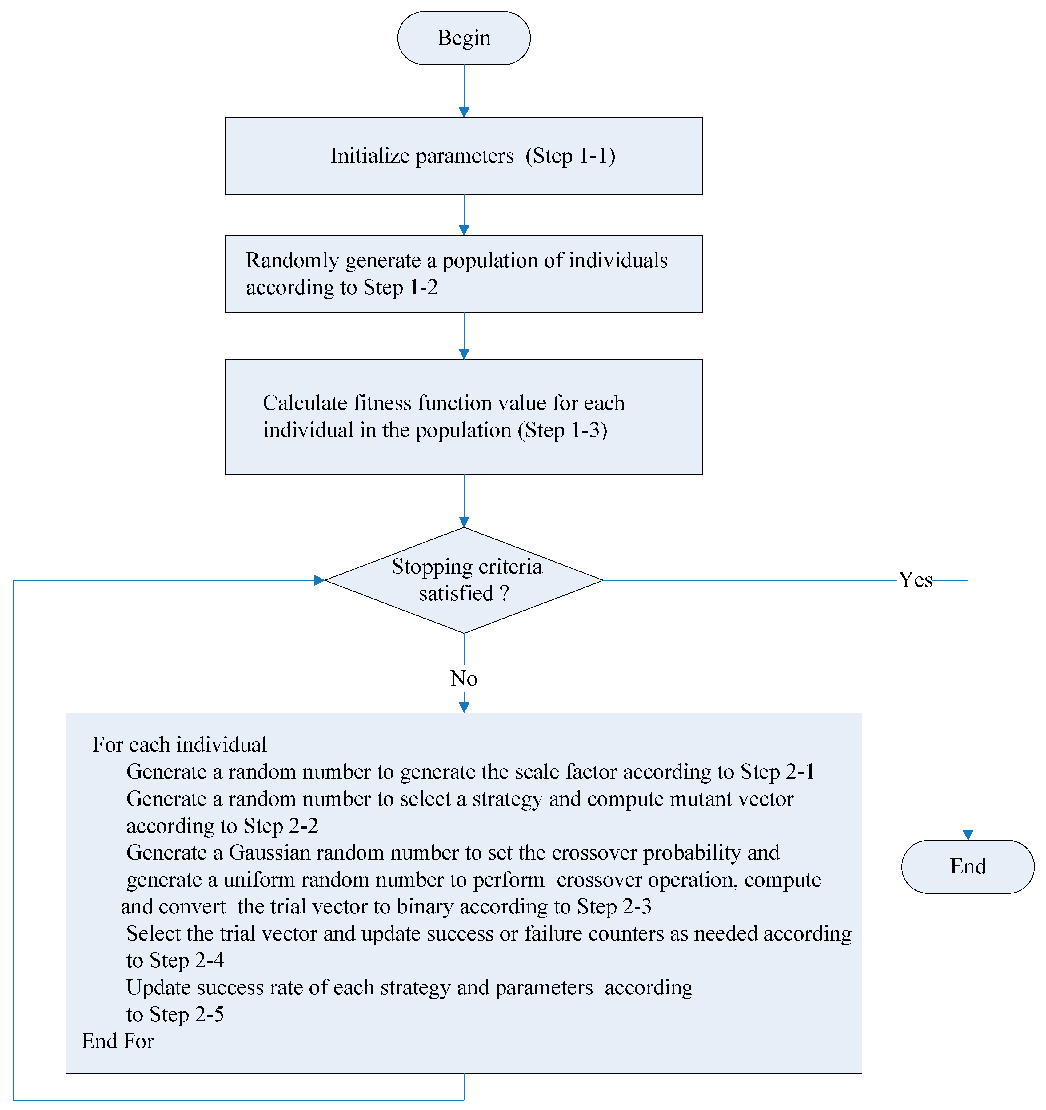The flow chart of the success rate-based self-adaptive metaheuristic algorithm is shown in Figure 1.

$$v_{(g+1)in}=z_{g{r}_{1}n}+F_i(z_{g{r}_{2}n}-z_{g{r}_{3}n})$$

(18)

$$v_{(g+1)in}=z_{gin}+F_i(z_{gbn}-z_{gin})+F_i(z_{g{r}_{1}n}-z_{g{r}_{2}n})+F_i(z_{g{r}_{3}n}-z_{g{r}_{4}n})$$

(19)

As we use two mutation strategies, a mutation strategy is referred to as $s$, where $s\in \{1,2\}$. In the proposed algorithm, the number of times that a mutation strategy $s$ successfully improves the performance is stored in variable $S_s$. The number of times that a mutation strategy $s$ fails to improve the performance is stored in variable $U_s$. The success rate of strategy $s$ is $w_s=\frac{S_s}{S_s+U_s}$, where $s\in \{1,2\}$. The parameter $f_p$ used to select the probability distribution to generate the scale factor and select the mutation strategy is calculated by $f_p=\frac{w_1}{w_1+w_2}$. A list $L$ is used to store the crossover probability $c{r}_i$ that successfully improves performance by executing the statement $L\leftarrow L\cup \left\{c{r}_i\right\}$. The list $L$ is used to update the parameter $cr$ by $cr=\frac{{\displaystyle \sum _{k\in \{1,2,\dots ,\left|L\right|\}}^{}L(k)}}{\left|L\right|}$, which is used to generate the crossover probability $c{r}_i$ in the next generation.

The discrete self-adaptive metaheuristic algorithm based on success rate and differential evolution is listed in Algorithm 1.

Algorithm 1: Discrete Self-Adaptive Metaheuristic Algorithm based on Success Rate and Differential Evolution

Step 1: Initialize the parameters and population of individuals

Step 1-1: Initial the parameters

$cr=0.5$

$f_p$ = 0.5

Step 1-2: Generate a population with $NP$ individuals randomly

Step 2: Evolve solutions

For $g=1 to G$

For $i=1 to NP$

Step 2-1: Generate a uniform random number $r$ from uniform distribution $U(0,1)$ ranging from 0 to 1

$F_i=\{\begin{array}{l}{r}_1, where r_1 is a Gaussian random number with N(\mu ,{\sigma }_1^2) if r<f_p\\ r_2, where r_2 is a uniform random number sampled from U(0,1) otherwise\end{array}$

Step 2-2: Generate a uniform random number $r$ from uniform distribution $U(0,1)$ ranging from 0 to 1

Calculate the mutant vector $v_{gi}$ as follows.

For $n\in$1, 2, …, $N$

$v_{(g+1)in}=\{\begin{array}{l}{z}_{g{r}_{1}n}+F_i(z_{g{r}_{2}n}-z_{g{r}_{3}n}) if r<f_p\\ v_{(g+1)in}=z_{gin}+F_i(z_{gbn}-z_{gin})+F_i(z_{g{r}_{1}n}-z_{g{r}_{2}n})+F_i(z_{g{r}_{3}n}-z_{g{r}_{4}n}) otherwise\end{array}$

$s=\{\begin{array}{l}1 if r<f_p\\ 2 otherwise\end{array}$

End For

Step 2-3: Generate a trial vector $u_{gi}$

Generate a Gaussian random number $c{r}_i$ with distribution $N(cr,{\sigma }_2^2)$

For $l\in$1, 2, …, $N$

Generate a uniform random number $r$ from uniform distribution $U(0,1)$ ranging from 0 to 1

$u_{gil}=\{\begin{array}{l}{v}_{gil} if r<c{r}_i\\ z_{gil} otherwise\end{array}$

${\overline{u}}_{gil}\leftarrow Convert2Binary(u_{gil})$

End For

Step 2-4: Update the individual and success/failure counters

If $H_1({\overline{u}}_{gi})\ge H_1(z_{gi})$

$z_{(g+1)i}$ = $u_{gi}$

$L\leftarrow L\cup \left\{c{r}_i\right\}$

$S_s=S_s+1$

Else

$U_s=U_s+1$

End If

End For

Step 2-5: Update the parameters as needed

If $g>LP$

$w_1=\frac{S_1}{(S_1+U_1)}$

$w_2=\frac{S_2}{(S_2+U_2)}$

$f_p=\frac{w_1}{w_1+w_2}$

$cr=\frac{{\displaystyle \sum _{k\in \{1,2,\dots ,\left|L\right|\}}^{}L(k)}}{\left|L\right|}$

End If

End For

5. Results

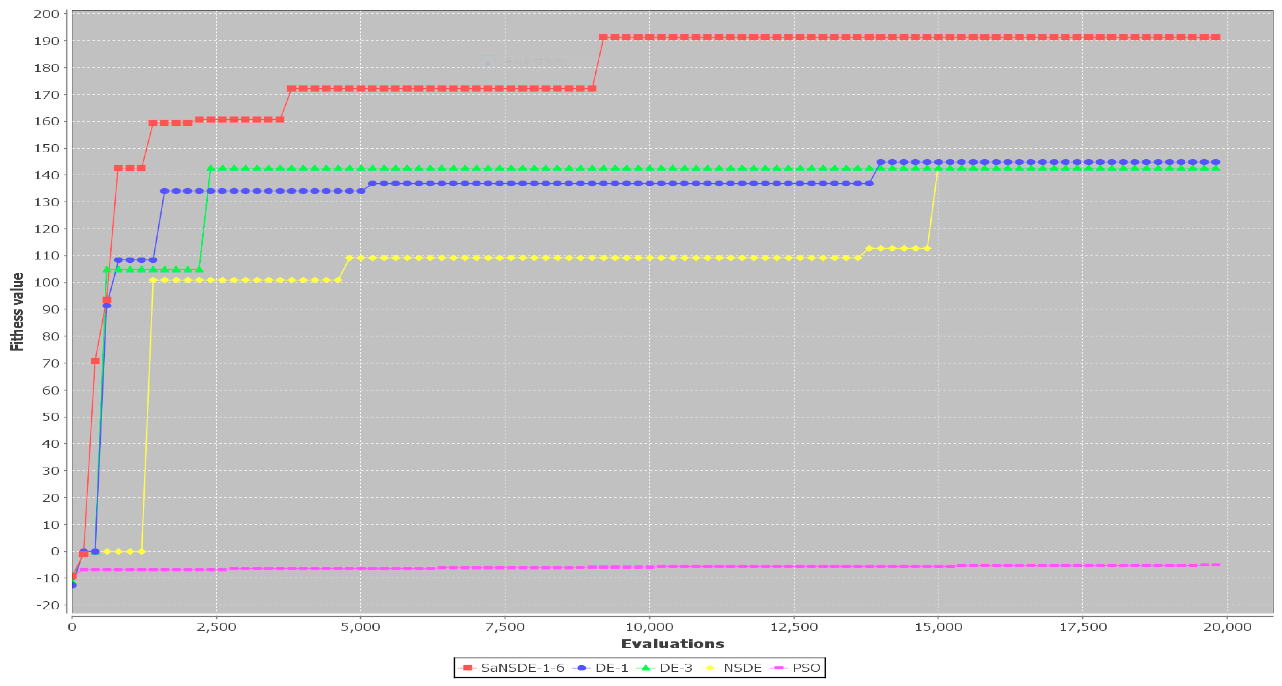
As the goal of this paper is to improve the performance of the quality of solutions for the DGRP and improve the convergence rate (the number of generations) for finding the best solutions, verification by the results of experiments is needed to demonstrate the advantage of the proposed algorithm. In this section, the results of experiments obtained by applying the algorithm developed in this paper will be analyzed. Our analysis focuses on two algorithmic properties: performance and convergence rate.

The evaluation process of the algorithms can be divided into five steps. The first step is to select the performance metrics for comparing different algorithms, the second step is to create instances for the DGRP, the third step is to set the parameters for different algorithms, the fourth step is to apply different algorithms to solve each instance of the DGRP and the fifth step is to calculate the performance metrics under consideration based on the results of experiments and compare all algorithms. For the first step, the performance metrics for comparing different algorithms include the average fitness function values, the average number of generations to find the best solutions and the average computation time to find the best solutions. For the second step, the locations of drivers and passengers are randomly generated based on a selected geographical area in Taichung City, which is located in the central part of Taiwan. The number of drivers and the number of passengers are increased gradually to generate instances of the DGRP with different size. For the third step, the parameters for PSO, NSDE, DE-1 and DE-3 are the same as the ones used in [13]. The parameters for SaNSDE-1-6 are specified later in this section. For the fourth step, we apply SaNSDE-1-6 ten times to solve each instance of the DGRP. As the results of applying PSO, NSDE, DE-1 and DE-3 to Case 1 through Case 10 are available in [13], we apply PSO, NSDE, DE-1 and DE-3 ten times to solve to Case 11 through Case 14. For the fifth step, we first calculate the average fitness function values, the average number of generations to find the best solutions and the average computation time to find the best solutions based on the results obtained. We then compare all algorithms based on the performance metrics mentioned above.

In [13], ten algorithms were developed to solve the DGRP. The study of [13] indicates that the NSDE, DE-1, DE-3 and PSO are the top four solvers among the ten algorithms for solving the DGRP in terms of performance and convergence rate (the number of generations to find the best solutions).

To illustrate effectiveness of the algorithm proposed, the experiments include Test Case 1–10 (available at [40]) used in [13] and Test Case 11–14 (available at [41]) to compare with the existing algorithms for the DGRP. To illustrate superiority of the algorithm proposed in terms of scalability with respect to problem size, we generated several test cases by increasing the problem size. We conducted these additional test cases by applying the algorithm proposed in this paper and the best four algorithms reported in [13]. We analyzed by comparing the results obtained by applying all of these algorithms to study the performance and convergence rate of these algorithms as problems grow.

As the effectiveness of evolutionary algorithms depends on the population size parameter, we conducted two series of experiments. The population size parameter of the first series of experiments is 30. The population size parameter of the second series of experiments is 50. The values of algorithmic parameters used by each algorithm are listed in

Table 2. Parameters for different algorithms and test cases.

Algorithm	Parameters for Case 1 through Case 10	Parameters for Case 11 through Case 14
SaNSDE-1-6	POP = 30, Gen = 1000, LP = 1000	POP = 50, Gen = 50,000, LP = 1000
DE-1	POP = 30, Gen = 1000, $CR$ = 0.5 $F$: a value arbitrarily selected from uniform (0, 2)	POP = 50, Gen = 50,000, $CR$ = 0.5 $F$: a value arbitrarily selected from uniform (0, 2)
DE-3	POP = 30, Gen = 1000, $CR$ = 0.5 $F$: a value arbitrarily selected from uniform (0, 2)	POP = 50, Gen = 50,000, $CR$ = 0.5 $F$: a value arbitrarily selected from uniform (0, 2)
NSDE	POP = 30, Gen = 1000, $CR$ = 0.5, $F_i$ = $0.5r_1+0.5$, where $r_1$ is a random value with Gaussian distribution $N(0,1)$.	POP = 50, Gen = 50,000, $CR$ = 0.5, $F_i$ = $0.5r_1+0.5$, where $r_1$ is a random value with Gaussian distribution $N(0,1)$.
PSO	POP = 30, Gen = 1000, $c_1$ = 0.4, $c_2$ = 0.6, $\omega$ = 0.4	POP = 50, Gen = 50,000, $c_1$ = 0.4, $c_2$ = 0.6, $\omega$ = 0.4

. The number of generations parameter used by each algorithm is set to 1000 for Test Case 1 through Test Case 10. The number of generations parameter used by each algorithm is set to 50,000 for Test Case 11 through Test Case 14.

Experiments based on the parameters in Table 2 for $NP$ = 30 were performed. The results were summarized in

Table 3. Fitness function values for discrete SaNSDE-1-6,DE-1, DE-3, NSDE and PSO algorithms with NP = 30; $r_D$ = $r_P$ = 0.1.

Case	D	P	SaNSDE-1-6	DE-1	DE-3	NSDE	PSO
1	3	10	32.998	32.998	32.998	32.998	32.998
2	5	11	63.615	63.615	63.615	63.615	63.615
3	5	12	41.715	41.715	41.715	41.715	41.2892
4	6	12	51.11	51.11	51.11	51.11	50.9085
5	7	13	30.063	30.063	30.063	30.063	28.4254
6	8	14	72.328	72.328	72.328	72.328	70.2629
7	9	15	89.03	89.03	89.03	89.03	80.8106
8	10	16	54.02	54.02	54.02	54.02	44.0023
9	11	17	74.05	74.05	74.05	74.05	49.356
10	12	18	50.9	50.0623	50.9	50.9	32.8349
11	20	20	112.906	112.906	112.906	112.906	97.7979
12	30	30	202.15	196.9089	200.1078	200.7964	141.6005
13	40	40	201.8256	190.1664	179.4244	186.6996	−1.5081
14	50	50	190.9436	137.1625	171.1756	161.3107	−3.9598

and

Table 4. Average number of generations for discrete SaNSDE-1-6,DE-1, DE-3, NSDE and PSO algorithms with $NP$ = 30; $r_D$ = $r_P$ = 0.1.

Case	D	P	SaNSDE-1-6	DE-1	DE-3	NSDE	PSO
1	3	10	9.6	16.6	19.8	15.6	64.6
2	5	11	19.2	32.2	36.9	29.1	299.6
3	5	12	29.4	39.7	47.6	43.3	394.5
4	6	12	19.6	43.8	50.3	44.1	320.9
5	7	13	16.7	31.8	44.1	37.3	304.1
6	8	14	20	48.3	67.8	39.6	375.6
7	9	15	60.8	101.4	135	70.7	553.6
8	10	16	48.2	61.3	78.6	59.5	447.5
9	11	17	53.9	59.7	65	64.2	580.7
10	12	18	106.4	136.8	146.3	94.3	489.3
11	20	20	191	436.5	817.1	542.5	21,314.5
12	30	30	1392.5	5691.5	16,065.1	14,417.2	21,742.3
13	40	40	18,439.777	15,185.8	27,574.4	27,260.1	22,734.2
14	50	50	19,390.5	17,131.7	22,745.3	36,742.7	25,822.2

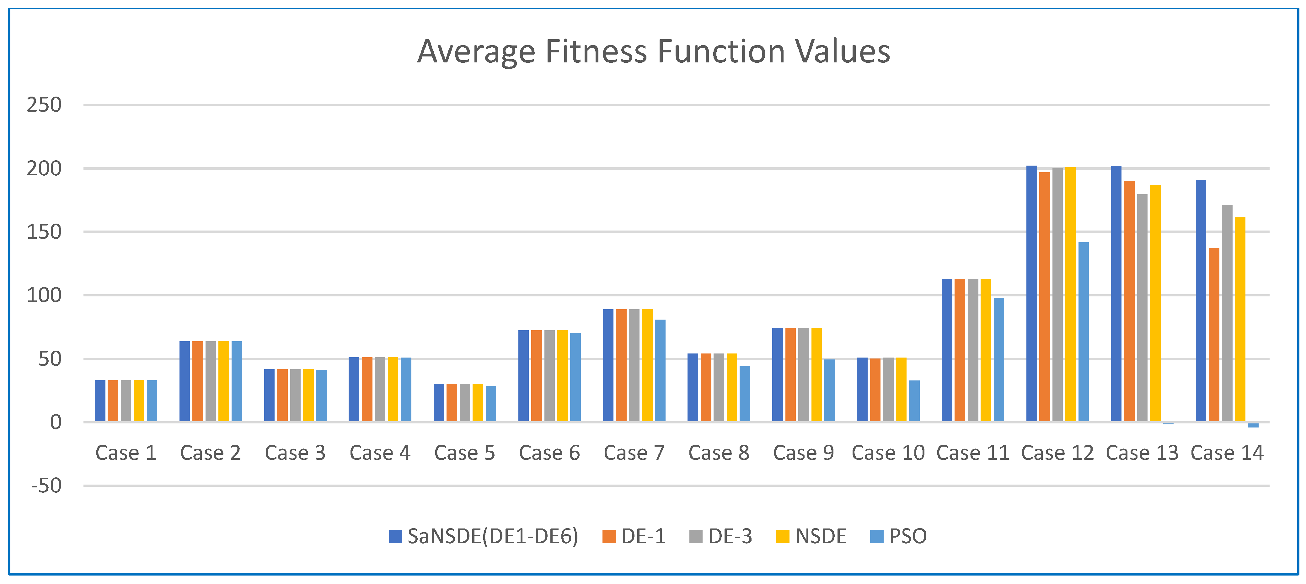
for $NP$ = 30. Table 3 shows the average fitness function value and Table 4 shows the average number of iterations to find the best solutions.

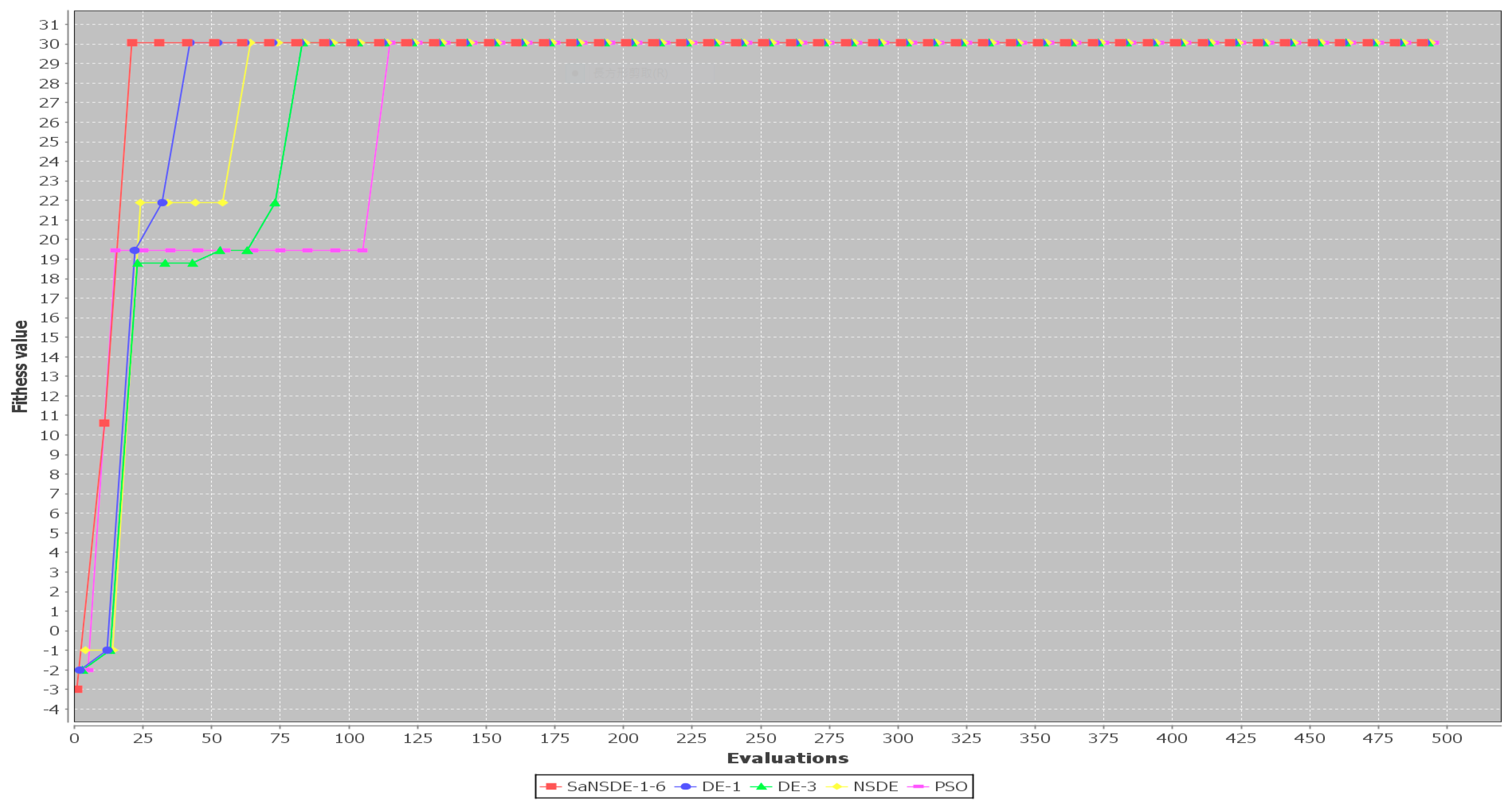
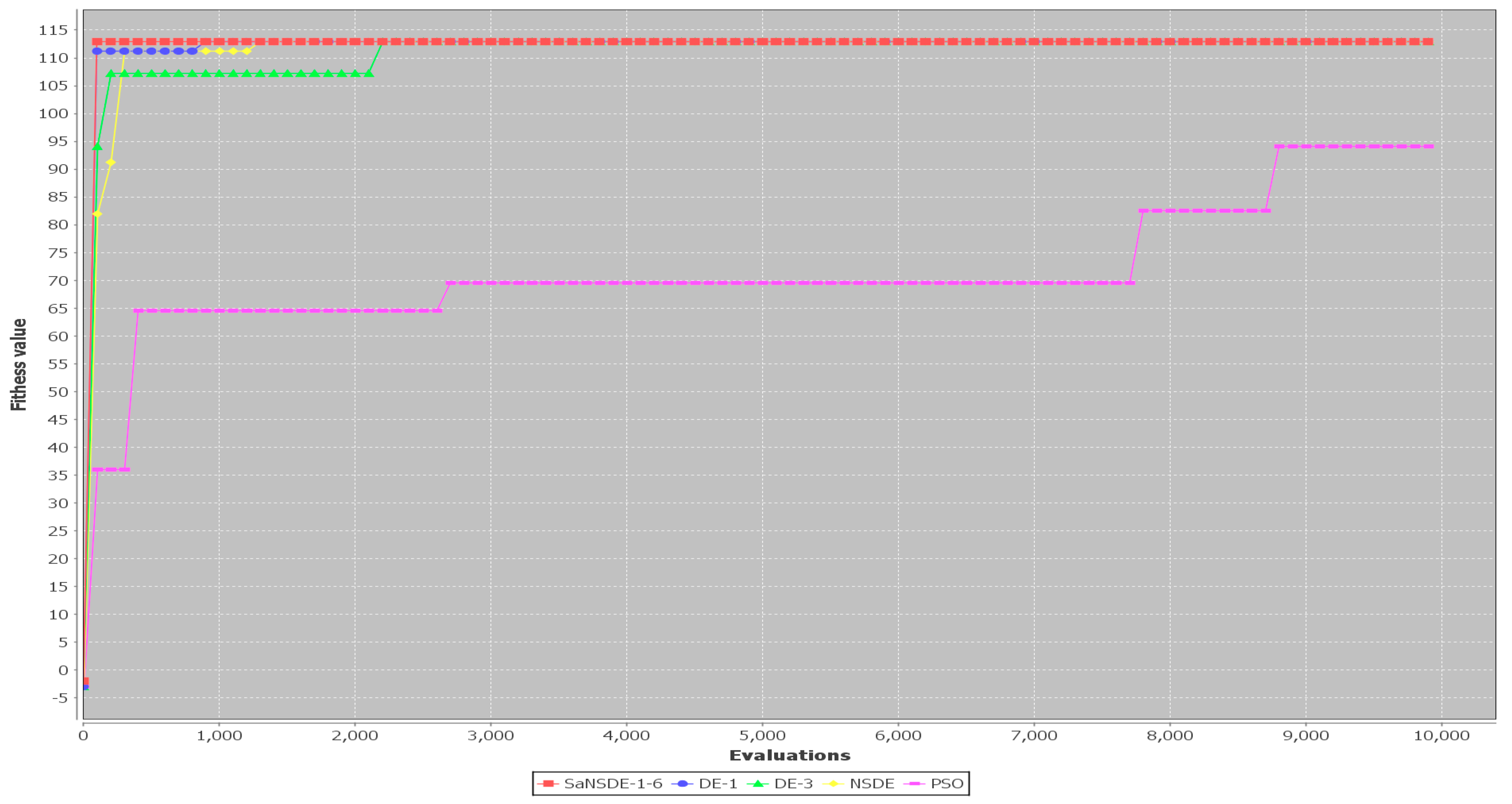
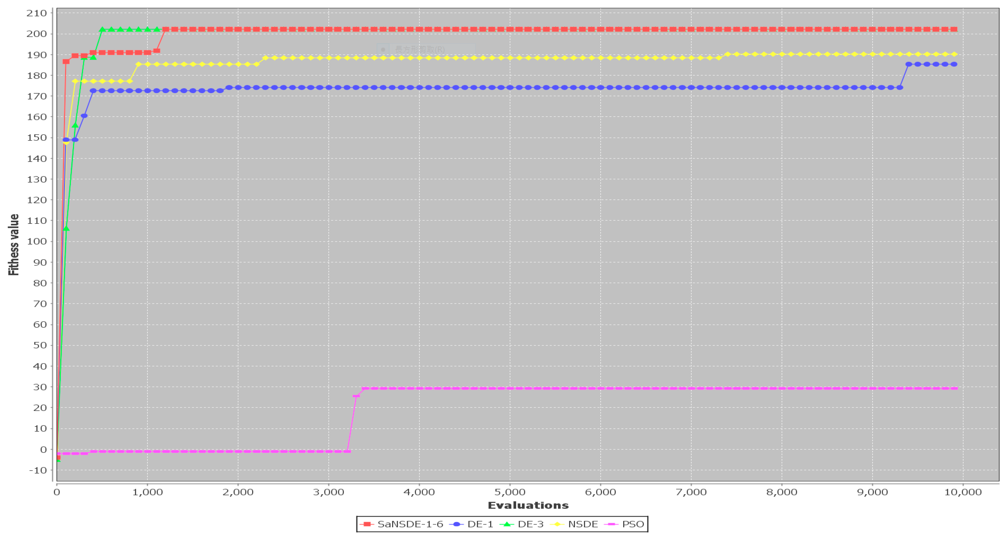
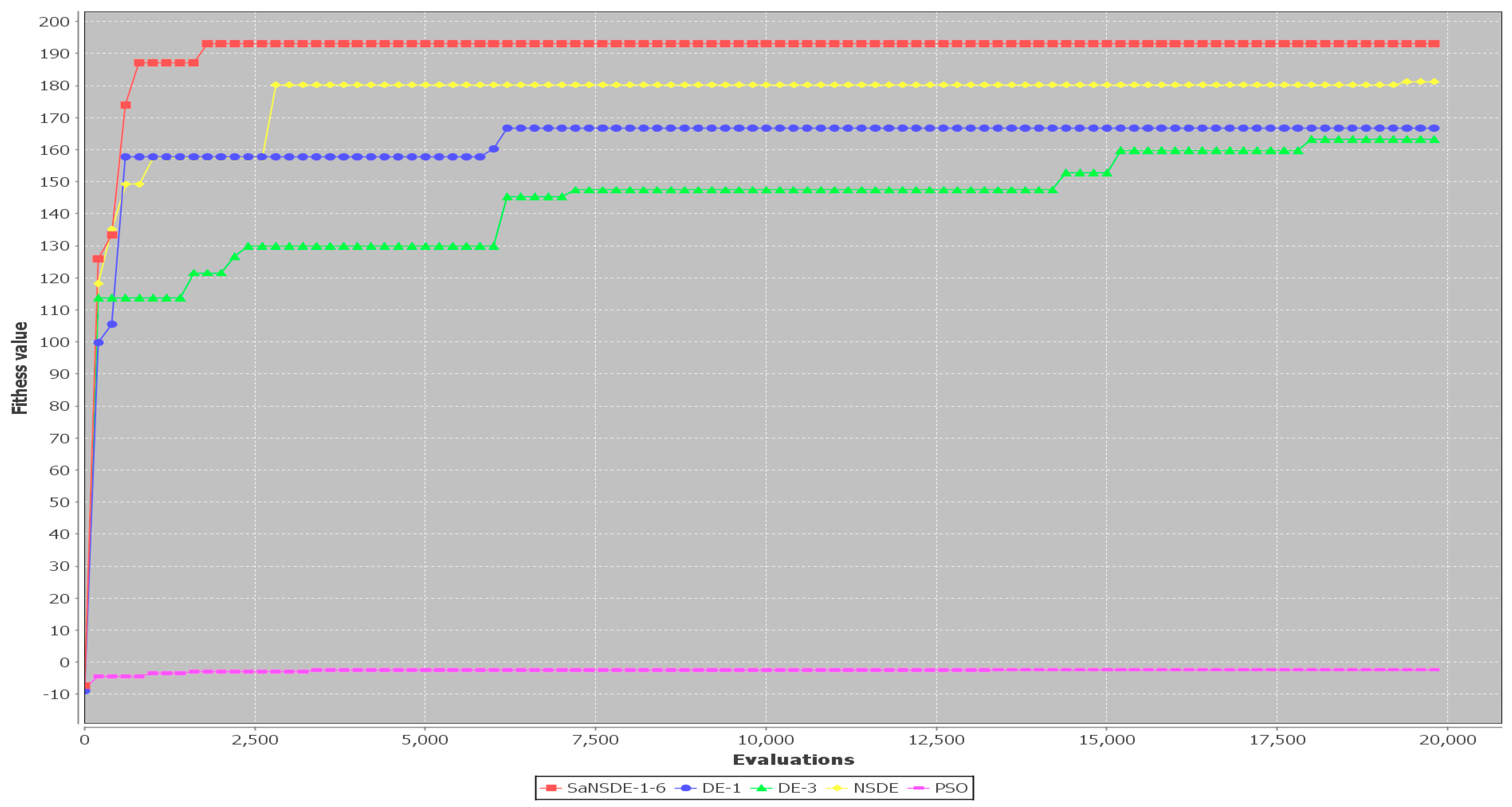
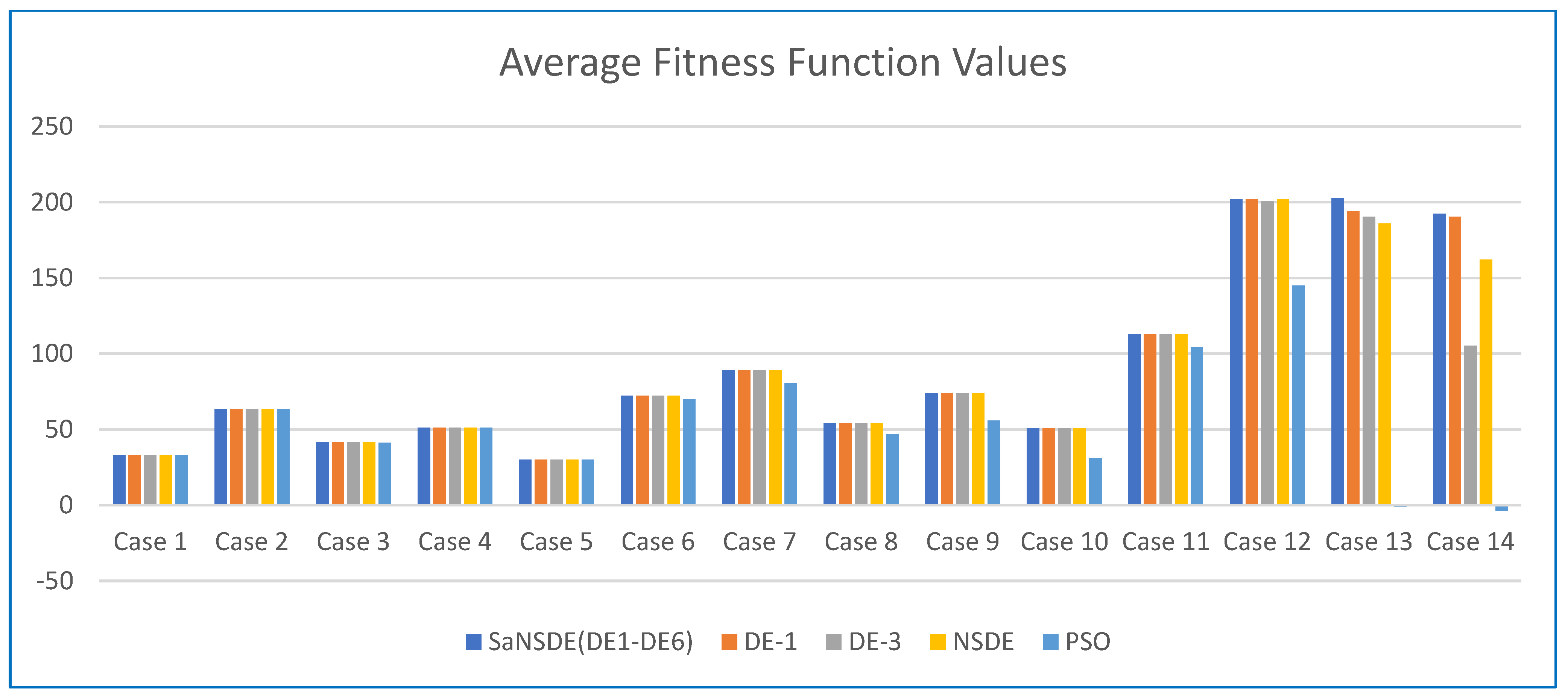
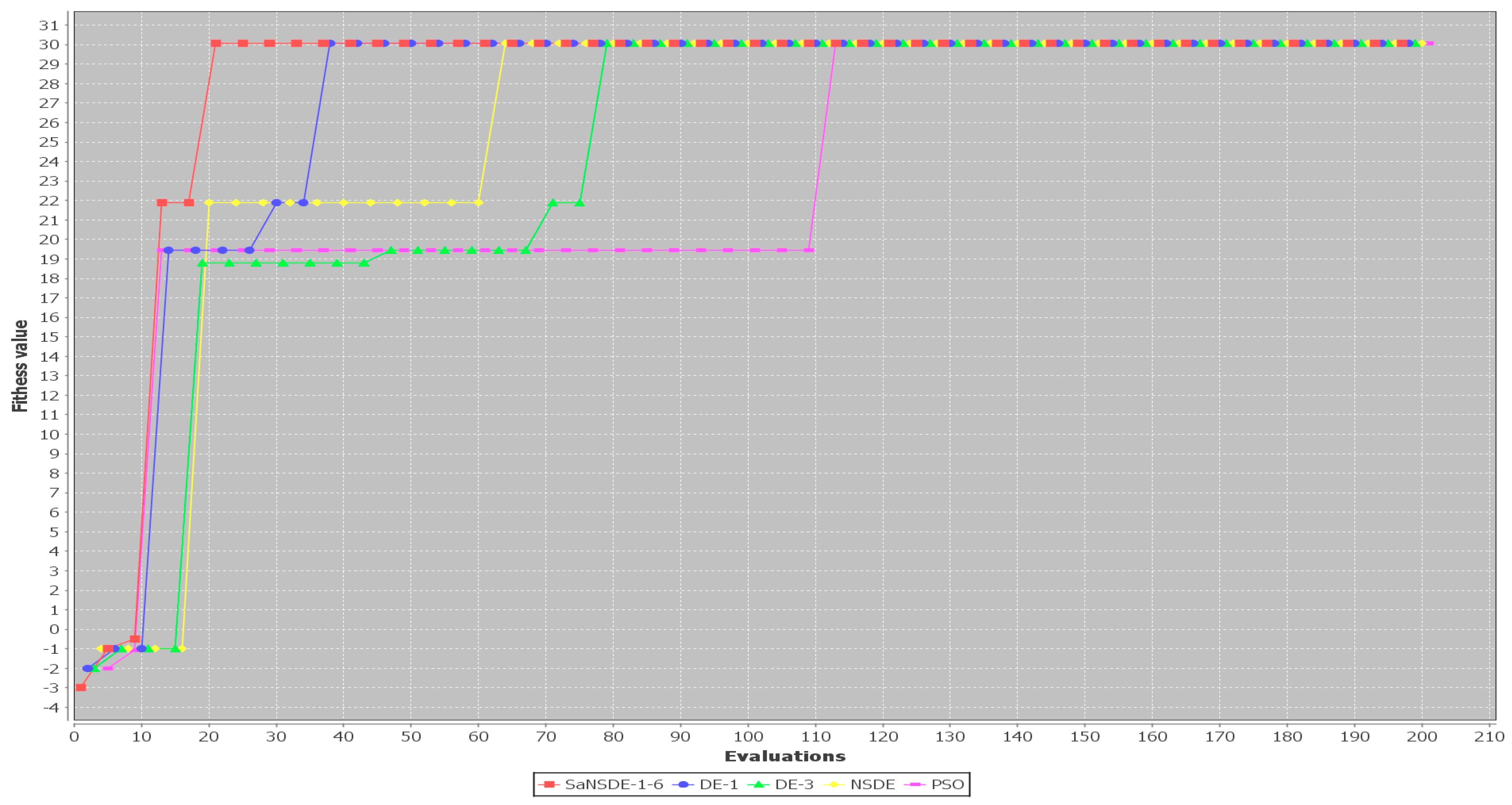
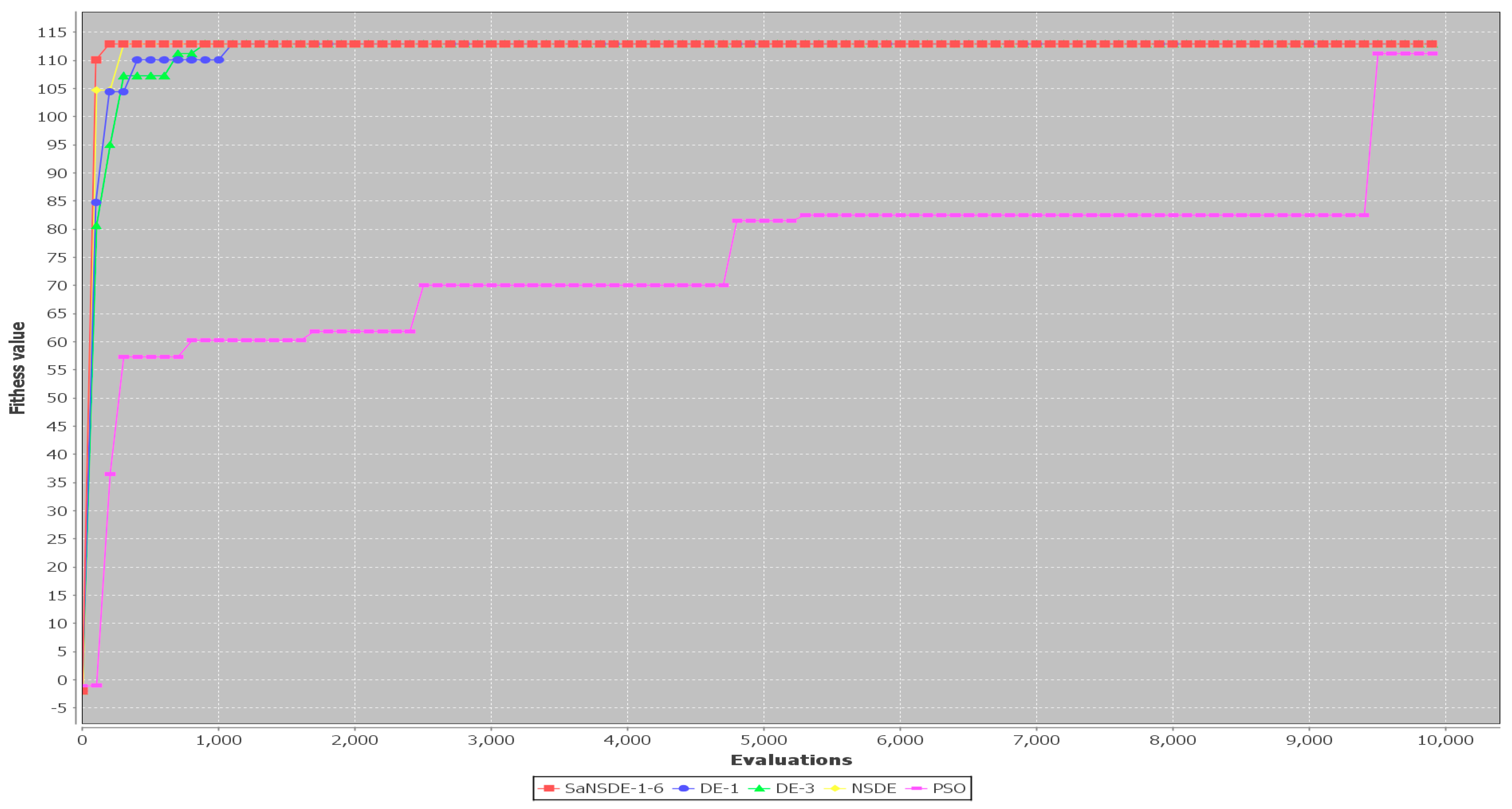
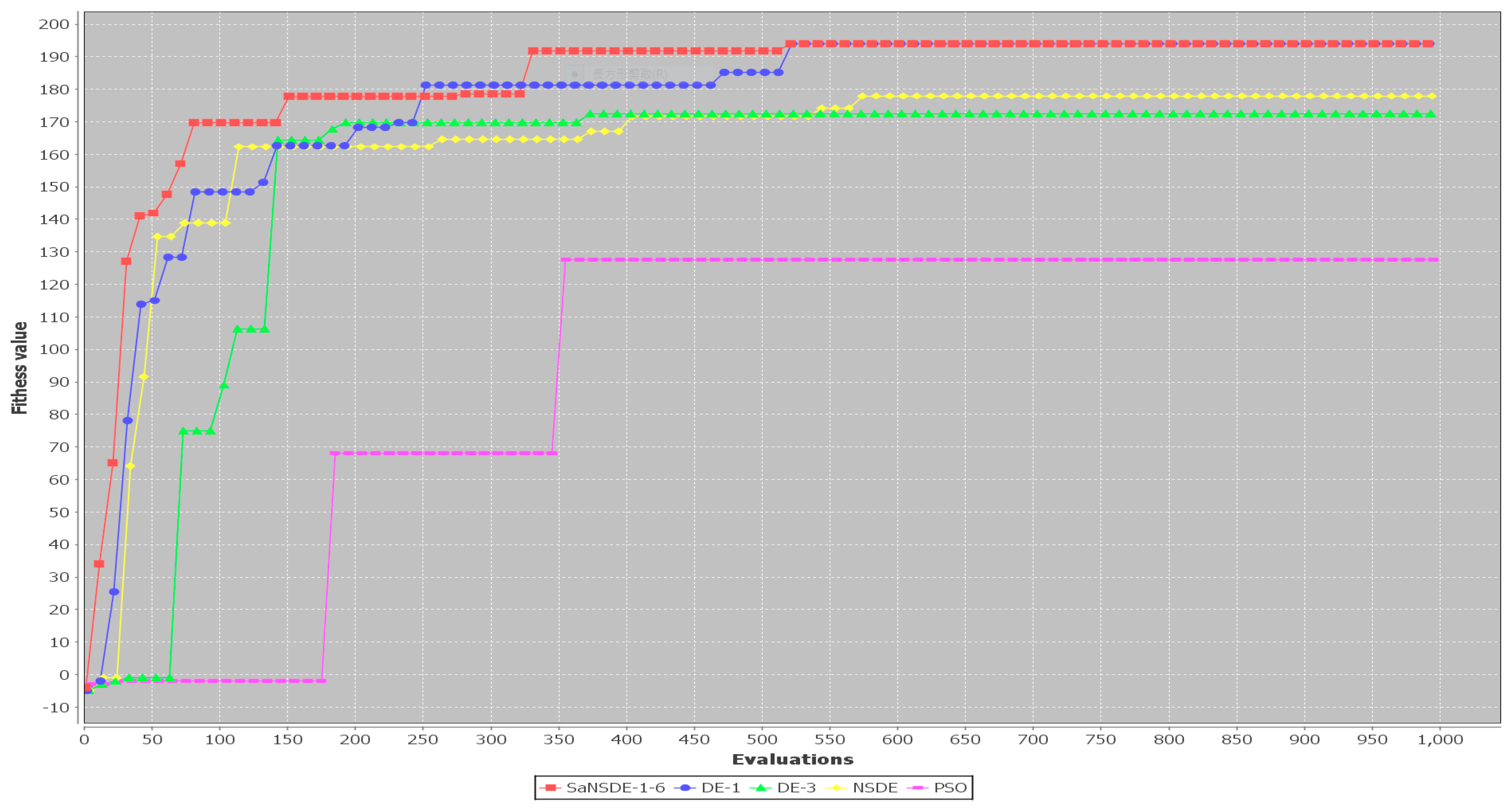
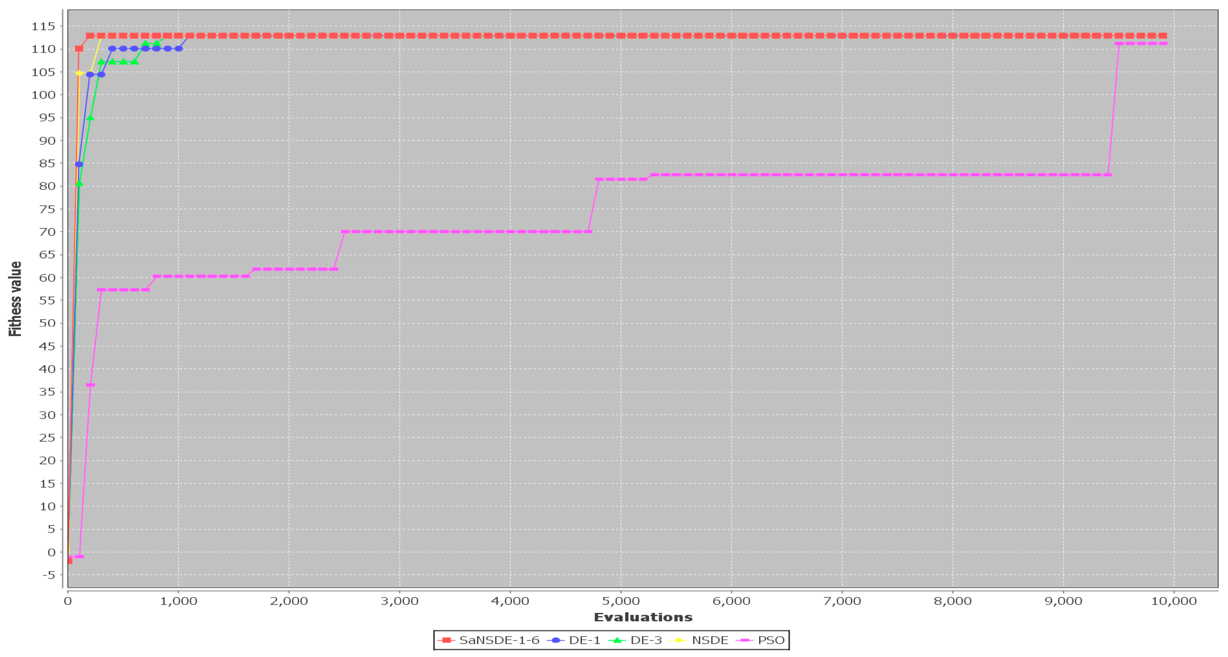
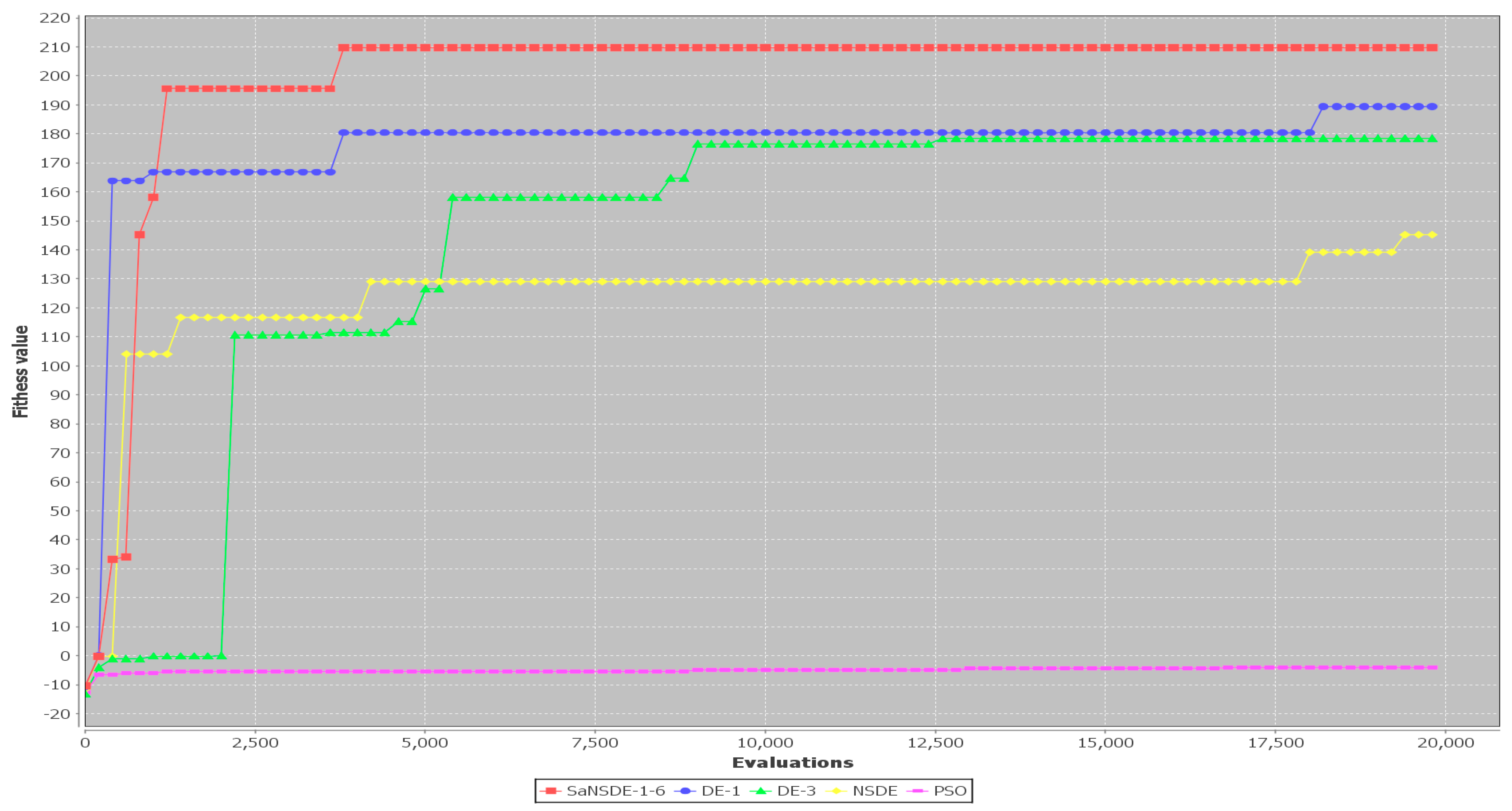
The results in Table 3 show that the top four algorithms are SaNSDE-1-6, NSDE, DE-1 and DE-3. For small test cases, including Case 1 through Case 11, the fitness function values obtained using SaNSDE-1-6, NSDE, DE-1 and DE-3 are the same. However, as the problem size grows, the average fitness function values obtained using SaNSDE-1-6 are significantly better than those obtained using NSDE, DE-1 and DE-3. For Case 12, the average fitness function value obtained using SaNSDE-1-6 is better than those obtained using NSDE, DE-1 and DE-3. The differences between the average fitness function value obtained using SaNSDE-1-6 and those obtained using NSDE, DE-1 and DE-3 are about 1% to 2%. For Case 12, the average fitness function value obtained using SaNSDE-1-6 is better than those obtained using NSDE, DE-1 and DE-3. For Case 13, the differences between the average fitness function value obtained using SaNSDE-1-6 and those obtained using NSDE, DE-1 and DE-3 are about 5% to 10%. For Case 14, the differences between the average fitness function value obtained using SaNSDE-1-6 and those obtained using NSDE, DE-1 and DE-3 are about 10% to 28%. In short, SaNSDE-1-6 outperforms NSDE, DE-1 and DE-3 in terms of scalability. To compare performance clearly, please refer to the bar chart shown in Figure 2 for the average fitness function values of Case 1 through Case 14.

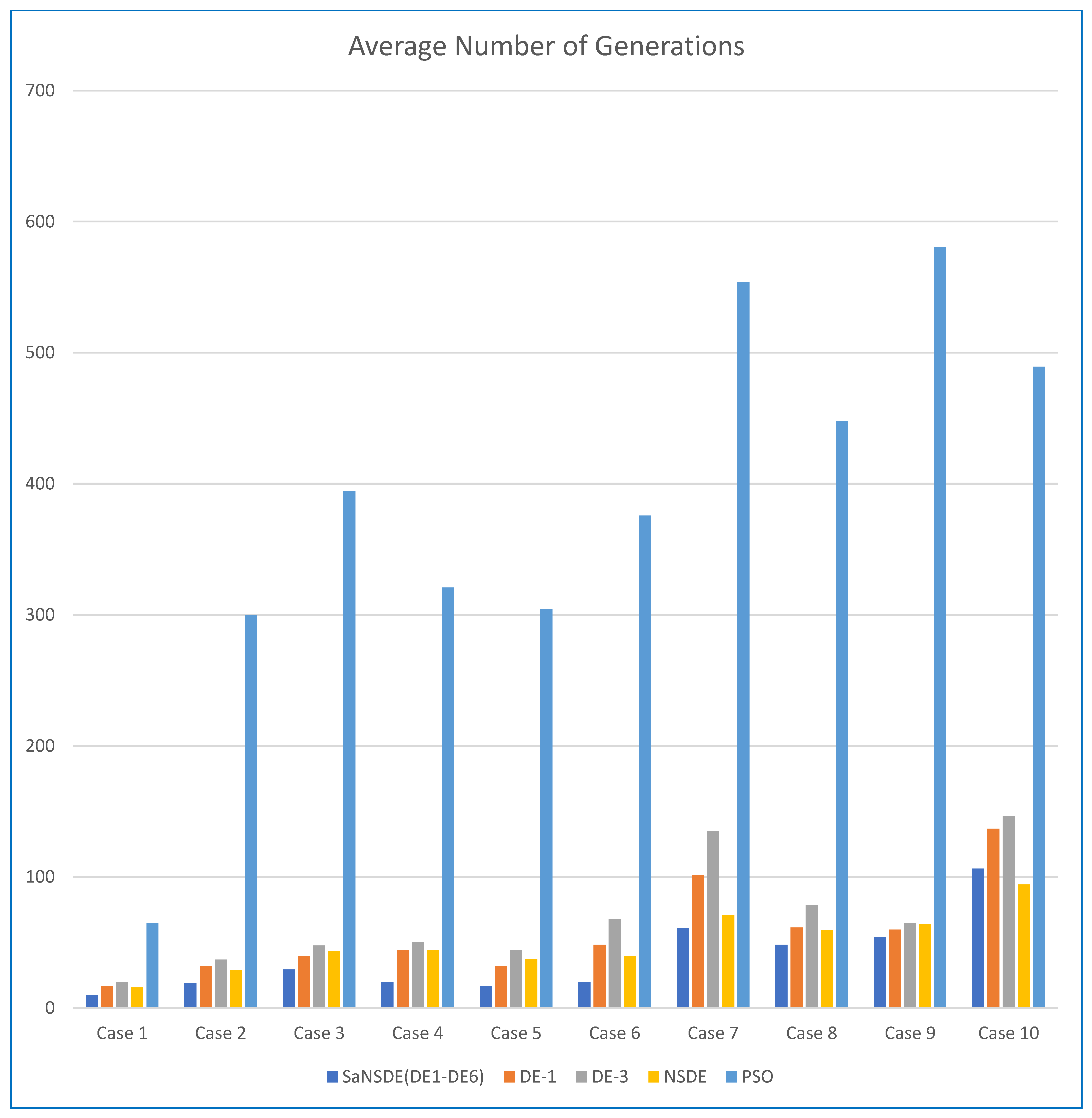
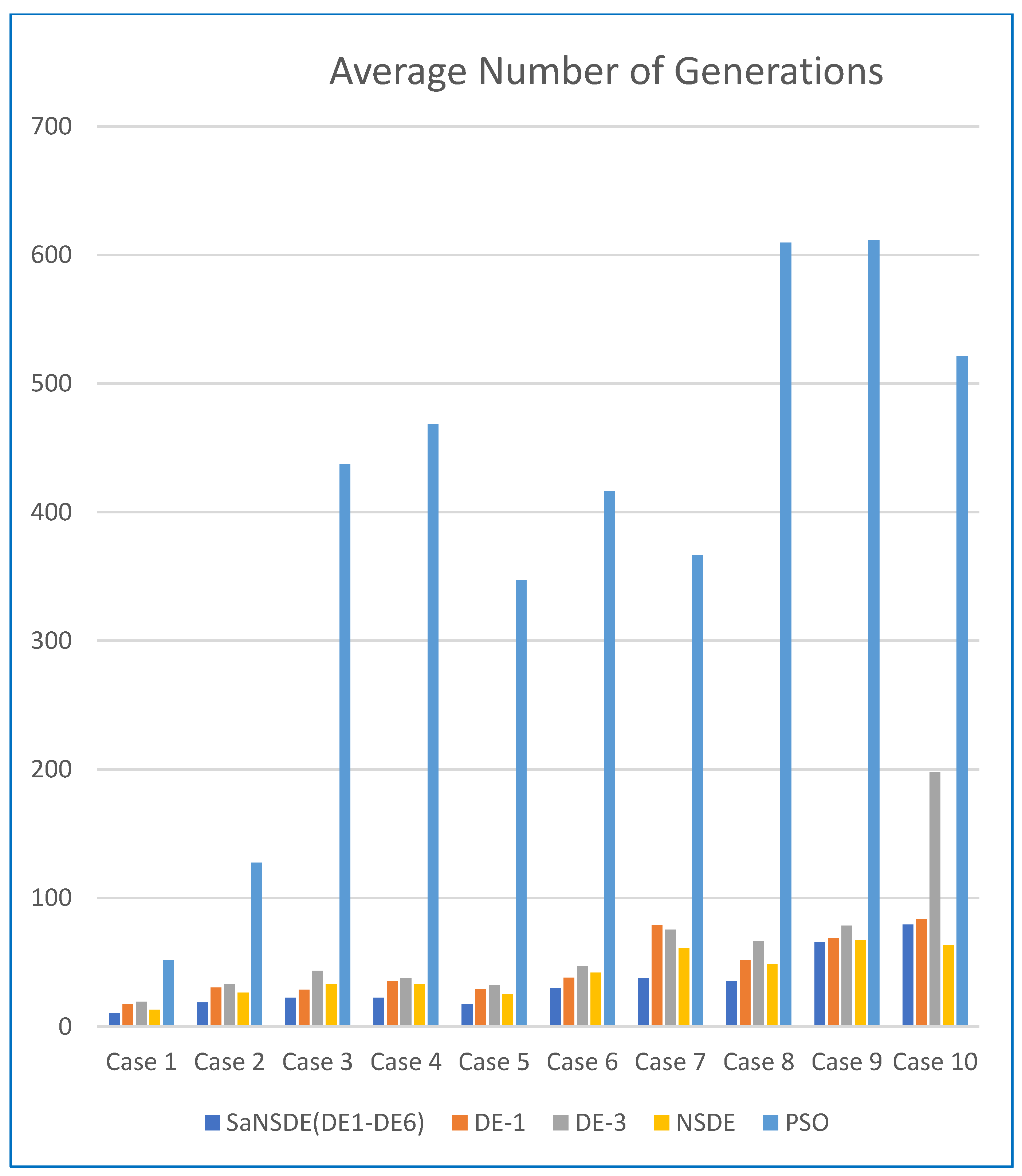
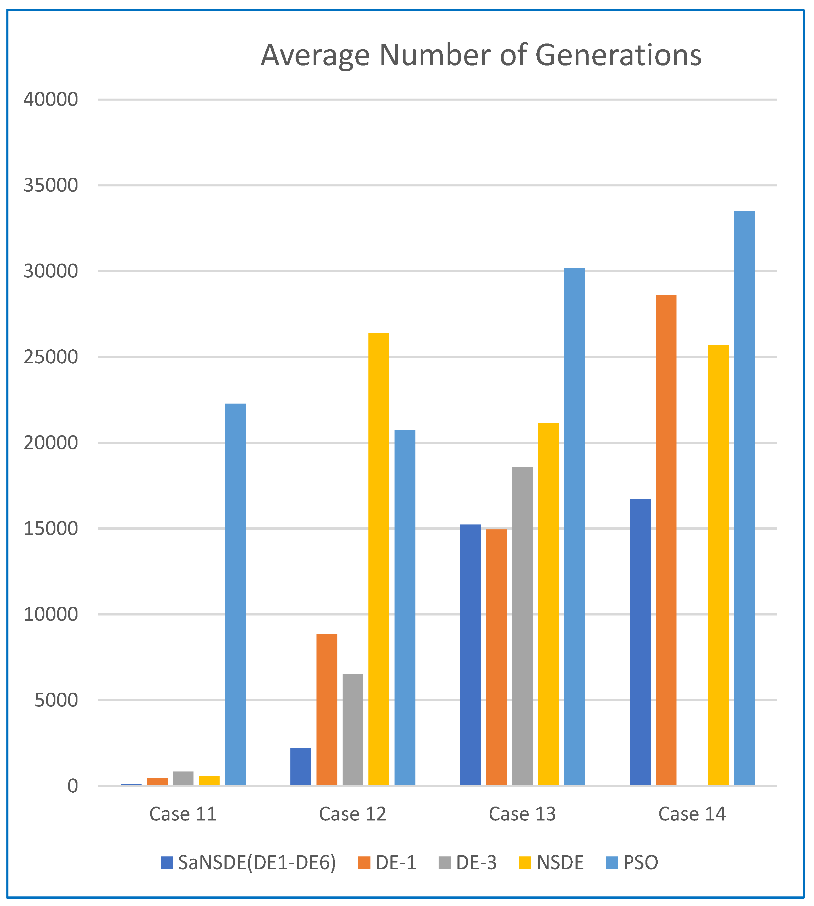
In terms of convergence rate (the number of generations to find the best solutions), the results in Table 4 indicate that the average numbers of iterations for SaNSDE-1-6 to find the best solutions are significantly less than those for NSDE, DE-1 and DE-3 to find the best solutions for most test cases (with some exceptions). This indicates that SaNSDE-1-6 outperforms NSDE, DE-1 and DE-3 in terms of convergence rate. 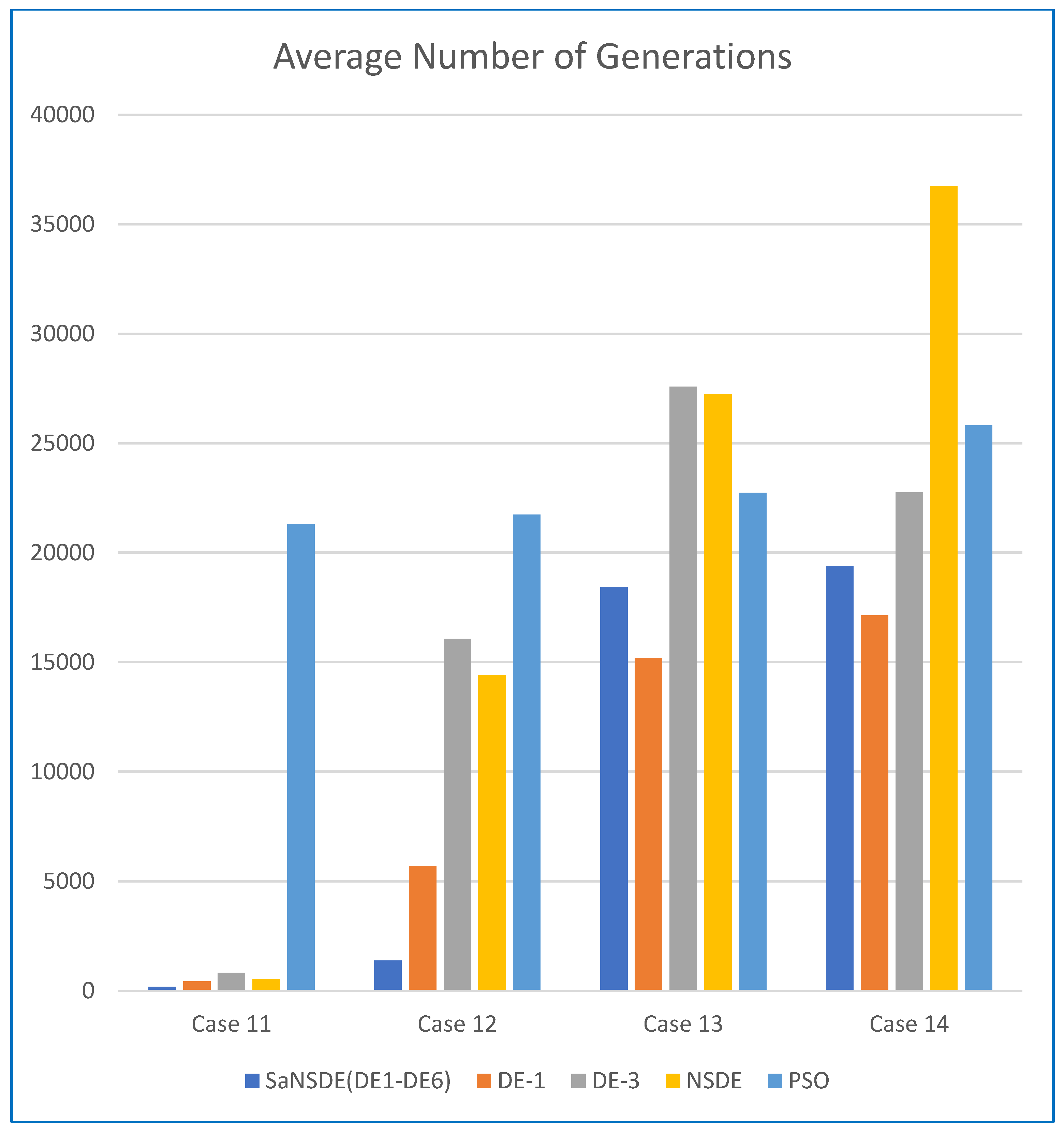To compare the convergence rate clearly, please refer to the bar chart shown in Figure 3 for the average number of generations of Case 1 through Case 10 and please refer to the bar chart shown in Figure 4 for the average number of generations of Case 11 through Case 14.

To verify the convergence rate for POP = 30, we show the results of several runs of Case 5, Case 11, Case 12, Case 13 and Case 14 in Figure 5, Figure 6, Figure 7, Figure 8 and Figure 9, respectively.

The results presented above are based on a comparison of the average number of generations. For the comparison of computation time, the results in

Table 5. Average computation time (in mini-second) for discrete SaNSDE-1-6,DE-1, DE-3, NSDE and PSO algorithms with $NP$ = 30; $r_D$ = $r_P$ = 0.1.

Case	D	P	SaNSDE-1-6	DE-1	DE-3	NSDE	PSO
1	3	10	11.494	5.8907	6.7182	7.3339	15.1677
2	5	11	31.0079	21.2555	18.0998	19.4591	118.2929
3	5	12	45.7525	22.0871	25.3382	26.1856	130.6768
4	6	12	42.0781	25.937	25.8155	29.1062	113.5842
5	7	13	28.2401	18.4303	22.264	16.7606	100.2475
6	8	14	48.7842	25.7381	34.9751	28.5755	132.6016
7	9	15	139.7892	73.5523	87.1861	55.5141	264.7854
8	10	16	111.0234	45.3785	54.5258	51.003	200.8072
9	11	17	152.6207	50.241	50.4531	64.2084	286.7221
10	12	18	236.4897	108.65	106.4809	87.0697	199.9287
11	20	20	798.39717	1134.249	2142.048	1496.592	45,171.44
12	30	30	21,158.007	17,419.87	49,393.98	48,106.86	51,932.66
13	40	40	2,116,465.2	60,483.27	113,286.7	119,378.3	66,539.42
14	50	50	3,198,096.1	90,395.02	118,089.5	144,559.9	87,874.68

indicate that the average computation time for SaNSDE-1-6 to find the best solutions is significantly less than that for PSO to find the best solutions for Case 1 through Case 9 and is greater than those of NSDE, DE-1 and DE-3 for Case 1 through Case 10. This indicates that SaNSDE-1-6 outperforms PSO in terms of computation time for Case 1 through Case 9 and NSDE, DE-1 and DE-3 outperform SaNSDE-1-6 in terms of computation time for Case 1 through Case 10. For Case 11, SaNSDE-1-6 outperforms PSO, NSDE, DE-1 and DE-3 in terms of computation time. For bigger cases, Case 12 through Case 14, PSO, NSDE, DE-1 and DE-3 outperform SaNSDE-1-6 in terms of computation time. As the experiments were done on the same platform as the one used in [13], which was an old laptop delivered in 2019 with Intel(R) Core(TM) i7 CPU, base clock speed of 2.6 GHz and16 GB of onboard memory, to compare different algorithms, the computation times of SaNSDE-1-6 are much longer for Case 12, Case 13 and Case 14. Obviously, a more powerful computer or a server class computer is required to apply the SaNSDE-1-6 algorithm.

Experiments based on the parameters in Table 2 for $NP$ = 50 were performed. The results were summarized in

Table 6. Fitness function values for discrete SaNSDE-1-6,DE-1, DE-3, NSDE and PSO algorithms with $NP$ = 50; $r_D$ = $r_P$ = 0.1.

Case	D	P	SaNSDE-1-6	DE-1	DE-3	NSDE	PSO
1	3	10	32.998	32.998	32.998	32.998	32.998
2	5	11	63.615	63.615	63.615	63.615	63.615
3	5	12	41.715	41.715	41.715	41.715	41.2892
4	6	12	51.11	51.11	51.11	51.11	51.11
5	7	13	30.063	30.063	30.063	30.063	30.063
6	8	14	72.328	72.328	72.328	72.328	69.9483
7	9	15	89.03	89.03	89.03	89.03	80.5986
8	10	16	54.02	54.02	54.02	54.02	46.8013
9	11	17	74.05	74.05	74.05	74.05	55.9356
10	12	18	50.9	50.9	50.9	50.9	31.1131
11	20	20	112.906	112.906	112.906	112.906	104.4808
12	30	30	202.15	201.8116	200.6549	201.8116	145.0514
13	40	40	202.4952	194.0284	190.4004	185.9914	−1.2835
14	50	50	192.343	190.4874	157.1781	162.1984	−3.6674

and

Table 7. Average number of generations for discrete SaNSDE-1-6,DE-1, DE-3, NSDE and PSO algorithms with $NP$ = 50; $r_D$ = $r_P$ = 0.1.

Case	D	P	SaNSDE-1-6	DE-1	DE-3	NSDE	PSO
1	3	10	10.1	17.6	19.2	12.9	51.5
2	5	11	18.7	30.2	33	26.4	127.3
3	5	12	22.3	28.7	43.3	32.9	437.2
4	6	12	22.5	35.4	37.4	33.2	468.6
5	7	13	17.7	29.3	32.2	24.8	247.1
6	8	14	30	38	47.1	41.9	416.4
7	9	15	37.5	78.9	75.4	61.3	366.4
8	10	16	35.3	51.5	66.3	48.6	609.5
9	11	17	65.6	68.7	78.4	67	611.5
10	12	18	79.4	83.6	197.9	63.1	521.5
11	20	20	98.6	469.5	829.5	565.5	22,275.7
12	30	30	2216.7	8847.1	6494.7	26,379.5	20,738.9
13	40	40	15,231.4	14,944.6	18,551.7	21,166.5	30,168.9
14	50	50	16,730.2	28,597.9	32,025.9	25,665.8	33,480.8

for $NP$ = 50. Table 6 shows the average fitness function values and Table 7 shows the average number of iterations to find the best solutions.

The results in Table 6 show that the top four algorithms are SaNSDE-1-6, NSDE, DE-1 and DE-3. For small test cases, including Case 1 through Case 11, the fitness function values obtained using SaNSDE-1-6, NSDE, DE-1 and DE-3 are the same. However, as the problem size grows, the average fitness function values obtained via SaNSDE-1-6 are significantly better than those obtained via NSDE, DE-1 and DE-3. For Case 12, the average fitness function value obtained via SaNSDE-1-6 is better than those obtained by NSDE, DE-1 and DE-3. The differences between the average fitness function value obtained via SaNSDE-1-6 and those obtained via NSDE, DE-1 and DE-3 are about 0.1674% to 0.73959%. For Case 12, the average fitness function value obtained via SaNSDE-1-6 is better than those obtained via NSDE, DE-1 and DE-3. For Case 13, the differences between the average fitness function values obtained via SaNSDE-1-6 and those obtained via NSDE, DE-1 and DE-3 are about 4.00326% to 7.9796%. For Case 14, the differences between the average fitness function value obtained via SaNSDE-1-6 and those obtained via NSDE, DE-1 and DE-3 are about 3.1171% to 46.403%. In short, SaNSDE-1-6 outperforms NSDE, DE-1 and DE-3 in terms of scalability. To compare performance clearly, please refer to the bar chart shown in Figure 10 for the average fitness function values of Case 1 through Case 14.

In terms of convergence rate (the number of generations to find the best solutions), the results in Table 7 indicate that the average numbers of iterations for SaNSDE-1-6 to find the best solutions are significantly less than those for NSDE, DE-1 and DE-3 to find the best solutions for most test cases (with some exception). This indicates that SaNSDE-1-6 outperforms NSDE, DE-1 and DE-3 in convergence rate. To compare the convergence rate clearly, please refer to the bar chart shown in Figure 11 for the average number of generations of Case 1 through Case 10 and please refer to the bar chart shown in Figure 12 for the average number of generations of Case 11 through Case 14.

To verify the convergence rate for POP = 50, we show the results of several runs of Case 5, Case 11, Case 12, Case 13 and Case 14 in Figure 13, Figure 14, Figure 15, Figure 16 and Figure 17, respectively.

The results presented above are based on comparison of average number of generations. The results in

Table 8. Average computation time (in mini-second) for discrete SaNSDE-1-6,DE-1, DE-3, NSDE and PSO algorithms with $NP$ = 50; $r_D$ = $r_P$ = 0.1.

Case	D	P	SaNSDE-1-6	DE-1	DE-3	NSDE	PSO
1	3	10	10.2156	10.1452	10.1662	8.4324	18.3854
2	5	11	31.0283	24.8503	24.4498	23.7312	57.3819
3	5	12	42.8796	23.849	32.7592	31.2488	212.022
4	6	12	33.3958	31.4915	29.161	33.3068	205.7338
5	7	13	33.6951	25.0836	25.8515	25.2025	105.7623
6	8	14	57.5261	32.3747	37.1701	42.8416	213.5017
7	9	15	117.5981	83.4787	78.1544	75.29	205.419
8	10	16	84.5311	65.2448	71.6938	71.265	385.2561
9	11	17	105.9706	87.5031	93.5826	86.378	413.8388
10	12	18	148.0639	101.1059	232.0098	96.711	400.4348
11	20	20	679.74567	1395.58	2805.873	1912.745	51,907.85
12	30	30	14,772.423	35,531.47	25,760.51	118,419.7	57,773.8
13	40	40	2,016,957.3	83,749.26	104,356	131,989.4	108,469.1
14	50	50	2,890,556.2	171,886.2	233,575.7	201,288.2	145,752.5

indicate that the average computation time for SaNSDE-1-6 to find the best solutions is significantly less than that for PSO to find the best solutions for Case 1 through Case 10 and is greater than those of NSDE, DE-1 and DE-3 for Case 1 through Case 10. This indicates that SaNSDE-1-6 outperforms PSO in terms of computation time for Case 1 through Case 10 and NSDE, DE-1 and DE-3 outperform SaNSDE-1-6 in terms of computation time for Case 1 through Case 10. For Case 11 and Case 12, SaNSDE-1-6 outperforms PSO, NSDE, DE-1 and DE-3 in terms of computation time. For Case 13 through Case 14, PSO, NSDE, DE-1 and DE-3 outperform SaNSDE-1-6 in terms of computation time. As the experiments to compare the different algorithms were done on the same platform as the one used in [13], which was an old laptop delivered in 2019 with Intel(R) Core(TM) i7 CPU, base clock speed of 2.6 GHz and16 GB of onboard memory, the computation times of SaNSDE-1-6 are much longer for Case 12, Case 13 and Case 14. Obviously, a more powerful computer or a server class computer is required to apply the SaNSDE-1-6 algorithm.

6. Discussion and Conclusions

In this paper, we applied the self-adaptation concept to develop an algorithm to improve the performance in finding solutions for the DGRP formulated in the previous study. The self-adaptation mechanism used in this paper attempts to identify a better strategy that can be selected in the future as the strategy for mutation with a higher probability. To identify a better strategy and the probability for serving as a mutation strategy in the future, the algorithm records the number of “success events” and the number of “failure events” in a learning period. The probability for serving as the mutation strategy is calculated based on the number of “success events” and the number of “failure events” in a learning period for each mutation strategy. A mutation strategy with a higher probability for serving as the mutation strategy will be selected with a higher probability. A mutation strategy with a lower probability for serving as the mutation strategy will be selected with a lower probability. In this way, the performance of the solution that is found can be improved more efficiently in terms of the average number of generations for most cases. However, due to the additional computation in each iteration, the computation time of SaNSDE-1-6 is much longer for big cases.

A mutation strategy with a higher probability for serving as the mutation strategy indicates that the ratio between the number of “success events” and the total number of “success events” and “failure events” is higher. It is expected that using a mutation strategy with a higher probability for serving as the mutation strategy tends to improve the performance of the solution that is found. The results presented in the previous section confirm that using a more effective mutation strategy with a higher probability for serving as the mutation strategy indeed improves the performance of the solution that is found significantly. The degree of improvement is case dependent. With $NP$ = 30, for Case 12, the improvement achieved using SaNSDE-1-6 is about 1% to 2%. For Case 13, the improvement achieved using SaNSDE-1-6 is about 5% to 10%. For Case 14, the improvement achieved using SaNSDE-1-6 is about 10% to 28%. In short, SaNSDE-1-6 outperforms NSDE, DE-1 and DE-3 in terms of scalability. With $NP$ = 50, for Case 12, the improvement achieved using SaNSDE-1-6 is about 0.1674% to 0.73959%. For Case 13, the improvement achieved using SaNSDE-1-6 is about 4.00326% to 7.9796%. For Case 14, the improvement achieved using SaNSDE-1-6 is about 3.1171% to 46.403%. In short, SaNSDE-1-6 outperforms NSDE, DE-1 and DE-3 in terms of scalability. The bigger the problem size, the more significant the improvement.

In the real world, when one person fails to solve a problem alone, it might be easier to solve the problem by asking another person for help and working together. The reason is that one may consult the other and/or help each other when taking actions or making decisions. This way to solve a problem effectively is commonly used in our daily life. The results of the experiments presented in this paper are consistent with the abovementioned phenomena in the real world. In our self-adaptation mechanism, there are two strategies involved in the solution-finding processes. The selection of one strategy in the solution-searching processes is based on the success probability learned from the learning period. To verify the effectiveness of the self-adaptation mechanism, we carried out experiments by applying several standard algorithms and our proposed algorithm. Two different population sizes were used to perform the experiments. We compared the effectiveness of several single strategy algorithms and the self-adaptation-based algorithm. Our results indicate that the proposed algorithm based on the self-adaptation mechanism improves the performance and convergence rate in terms of the average number of generations required for finding the solutions for most cases. Although our proposed algorithm outperforms all of the other four algorithms in terms of performance and convergence rate for most cases, the computation time of the proposed algorithm is much longer for several big cases due to the additional computation in each iteration. The results of this study have two implications. First, the performance in solving the DGRP with two strategies and a self-adaptation mechanism is better than with one strategy. Second, although the performance in solving the DGRP can be improved and the average number of generations required for finding the solution is reduced, the computation time of the proposed algorithm is much longer than all of the other four algorithms for bigger instances. This implies that either a more powerful computer or a proper divide-and–conquer strategy to divide a big instance of the DGRP into small ones must be used before applying the proposed algorithm. The computational experience showing that the proposed self-adaptive algorithm outperforms the other four algorithms for the test cases in this paper sparks an interesting research question: does the proposed self-adaptive algorithm outperform the other four algorithms? This research question requires further study in the comparative analysis of the proposed algorithm. A comparative analysis of the algorithms studied in this paper for specific performance indicators is a challenging future research direction. Studies of other performance evaluation indicators for the proposed algorithm are another interesting future research directions. The other interesting future research direction is to extend the success rate-based self-adaptive scheme proposed in this study to other evolutionary approaches.