Heuristic Greedy-Gradient Route Search Method for Finding an Optimal Traffic Distribution in Telecommunication Networks

Abstract

Rapid growth in the volume of transmitted information has lead to the emergence of new wireless networking technologies with variable heterogeneous topologies. With limited radio frequency resources, optimal routing problems arise, both at the network design stage and during its operation. We propose an algorithm based on a minimum loss intensity (greedy-gradient algorithm) to search for optimal routes of information transmission in telecommunication networks. The relevance of the developed algorithm is determined by its practical use in data-transmitting modeling systems. The proposed algorithm satisfies several requirements, such as the speed of the calculations performed, the fulfillment of the conditions for its convergence, and its independence on the selected loss probability function, as well as on the network topology. The idea of the algorithm is a step-by-step recalculation of metrics based on derivatives of the loss intensity function with simultaneous redistribution of information flows along the routes determined by the Floyd algorithm. The comparative efficiency of the proposed algorithm is demonstrated by computational experiments on various network topologies (up to 100 nodes) with various traffic intensities.

1. Introduction

The efficiency of using communication-channel resources is one of the most important problems of the telecommunication industry, since it enables us, on the one hand, to maximize the use of network resources, thereby increasing the profitability of the services provided, and, on the other hand, to ensure improved quality of service indicators by reducing delay time and probability losses.

For the efficient use of network resources in telecommunication networks, routing protocols dynamically alter the routes of information flows [1,2,3,4]. When developing a routing protocol, two factors are essential: the choice of optimality criterion for the route search method and the rate of changes in the network topology. The algorithm for finding the optimum of the objective function (criterion) should be many times faster than changing the network topology. The classic optimality criterion can be considered an optimal multipath routing according to the criterion of total delay time, described by the authors of [5]. Firstly, the intention is to find a set of simple routes between each pair of ”Sources” and ”Destinations”. Yen’s algorithm [6] is mostly used for this purpose as it enables the search for k-shortest paths. The disadvantage of this approach is the necessity to find all pairs of loopless routes between all pairs of ”Sources” and ”Destinations”, and that leads to a rapid complication of the optimization problem due to an increase in the number of state variables while providing an optimal solution. The situation can be improved by selecting only those routes satisfying certain criteria [7,8,9,10,11]. As a rule, such criteria are specified in the form of graph weights that reflect certain characteristics of the channel; such algorithms can also be used as independent ones. Another approach to the route selection is finding routes that do not have common edges, or the set of common edges is minimal [12].

The optimality criterion in [5] is the total delay time due to delays in the network device interface buffer. Based on the found routes of information flows, the total flow through each communication channel is determined. Afterwards, using the delay time equation for the M/M/1 queuing system, it is possible to estimate the objective function as the sum of all delay times in all channels. This approach with various modifications is used in many works, where a certain cost function is selected as an optimality criterion, which depends on the total flow [13,14,15], thereby causing linear and nonlinear programming problems. Such approaches are valid in the case of no information loss or in the case when the losses can be neglected, since in such cases it is possible to obtain the objective function in an explicit form with a linear set of constraints (inequalities). An alternative to mathematical models based on routes are mathematical models based on flows in communication channels [16], which, starting from a certain graph density, have a lower dimension (fewer number of state variables) than models based on flows. The closest concepts to the algorithm proposed in this paper have been presented in [17,18], which consider cell losses in the ATM network.

The relevance of the problem being solved is due to the emergence of new types of wireless networks with variable topologies, where the solution of routing problems is especially important due to limited radio frequency resources. Such networks include FANAET and MANET, which are satellite networks in low and medium orbits. Such interest in this area of communication systems is associated with the significant shortcomings of existing routing algorithms used in traditional IP networks, which researchers are trying to eliminate, for example:

-

inefficient use of network resources [19,20,21];

-

lack of prompt response to overloads when generating traffic and changing the network topology in existing satellite routing protocols [1,22,23,24,25,26,27,28,29,30];

-

inability to work with different types of traffic [19,31];

-

focusing on a single criteria when solving optimization problems with multiple objectives [19,21,22,23,24,25,26,27,28,29,30,31].

In addition to various problem settings for finding optimal routes, there are various methods to find them: heuristic algorithms [19,28,29], greedy algorithms [21], gradient methods [31], reinforcement learning [20], and neural networks [23]. In [3], the authors discuss the importance of global adaptive routing in large-scale systems with a large coverage area. For global adaptive routing, the choice of optimal routes is usually based on local information, such as line occupancy and approximate overload of information. However, existing heuristic-based adaptive routing algorithms often rely solely on local information, which can lead to inefficient solutions of the routing problem. Many recent papers are devoted to local routing, i.e., the route is determined for a single flow, without considering its influence on others. Hybrid algorithms that combine heuristic approaches with local search are also widely used for location problems [24,25,26], including location on networks, and the application of similar algorithmic combinations for traffic routing seems to be promising.

However, correct local actions do not always provide a proper solution from a global point of view. Approaches to global routing were proposed in [3,14,17]. However, these methods have several disadvantages. Since some of them are not sufficiently adapted for satellite networks [3,14], significant attention is paid to the probability of failures and delay time. Other authors [14,17] assume that there is a certain list of pre-defined routes for information delivery. However, determining this list is not a trivial task and, in general, it is difficult to specify in advance which routes will be used, and the total number of routes is growing so quickly that it is difficult to use all of them. Some researchers believe that the optimum of the unconstrained optimization problem is close to the optimum of the conditional optimization problem [17], which is not always true.

One of the main problems in finding optimal routes is the computational complexity that increases with the number of nodes used in the network. Furthermore, existing telecommunication networks often have a heterogeneous structure, which also complicates the process of route optimization.

Ref. [32] provides an overview of a large list of protocols used in wireless ad-hoc networks, and we can use them to solve the routing problem, since each of these protocols would enable us to find a set of information transmission routes; based on these, it would be possible to estimate the intensity of information loss.

We set a different goal for developing an optimization algorithm: finding routes that minimize losses, rather than using a routing protocol and then estimating the resulting losses. Such a problem in global traffic routing in telecommunication systems, and especially in satellite systems, had not yet been solved. Therefore, the development and application of effective algorithms for optimal routes while minimizing losses is an important issue. In this paper, we present a greedy-gradient algorithmic combination for solving such a problem and investigate the efficiency of the new approach by computational experiment.

The rest of this paper is organized as follows. In Section 2, we formulate the problem statement in a general form, and overview known methods of dynamic routing in the telecommunication networks. In Section 3, we describe our approach to solve the stated problem: the main optimization algorithm and supplementary algorithms. In Section 4, we summarize the results of computational experiments that demonstrate the stability of the proposed algorithm, its comparative efficiency, and capability of solving problems on larger networks. In Section 5, we provide conclusions to our work.

2. Problem Statement and Background

In this paper, we focus on the minimization of total losses. The telecommunication network is presented in the form of a directed graph, the parameters and keys of which are given below:

-

number of network nodes, N;

-

channel bandwidth capacity, ${\mu }_{ij}$, from the ith node to the jth one;

-

channel buffer size, $N_{ij}$, from the ith node to the jth one.

Let us assume that ${\mu }_{ij}=0$ if there is no communication channel between these nodes, and ${\mu }_{ij}=-1$ if the probability of information loss in the corresponding channel is 0. Therefore, e.g., if each node is connected to itself, there is no information loss.

The above-mentioned parameters characterize the network. Notion ”Target request” is introduced to describe the network. Let the ”Target request” be marked by g denoting the intensity of traffic transmitted from one node to another. Thus, e.g., writing $g=[16;7;200]$ means that one should deliver 200 units of information per second from the 16th to the 7th node.

We use the following notation:

-

number of target requests, Y;

-

matrix of target requests, $G=\left[g_i\right]$;

-

a specific target request, $g_i=[{start}_i;{finish}_i;Q_i]$, where $star{t}_i$ is the source node, $finis{h}_i$ is the recipient node, and $Q_i$ is the traffic intensity transmitted from the source node to the recipient node.

The intensity of losses when transmitting information over each channel can be determined using the following equation:

$$e_{ijk}=x_{ijk}p(x_{ij},{\mu }_{ij},N_{ij}).$$

(1)

The physical meaning of the variables in (1) is as follows: $e_{ijk}$ is the intensity of losses in the channel from the ith node to the jth one for the kth target request, $x_{ijk}$ is the intensity of information flow in the channel from the ith node to the jth one for the kth source, $x_{ij}$ is the total intensity of information flow in the corresponding channel, and $p(x_{ij},{\mu }_{ij},N_{ij})$ is the probability of information loss for the channel from the ith node to the jth node, which is usually a strictly increasing function due to physical fundamentals.

In this work, the objective function is defined as information losses when the required amount of information is delivered according to the target request matrices.

Currently, there are two possible approaches to formulating the traffic loss optimization problem [5,6,14,15,16,17,18,19,20]. According to the first approach, the information densities, $x_{ijk}$, are considered as variables. In this regard, we obtain a system of restrictions:

$$e_{jk}=\sum _{i=1}^n\left[x_{ijk}\frac{\left(1-\frac{{\sum }_t{x}_{ijt}}{{\mu }_{ij}}\right)}{1-{\left(\frac{{\sum }_t{x}_{ijt}}{{\mu }_{ij}}\right)}^{N_{ij}+1}}{\left(\frac{{\sum }_t{x}_{ijt}}{{\mu }_{ij}}\right)}^{N_{ij}}\right]=\sum _{i=1}^n{x}_{ijk}-\sum _{i=1}^n{x}_{jik}-c_{kj}+in{p}_{jk}.$$

(2)

where $c_{kj}$ is the total information rate provided when delivering data from the kth node to the jth one, $in{p}_{jk}$ are constants determined by the speed of information received from the jth source, $e_{jk}$ is the intensity of losses in the channel from the jth node to the kth one, and $x_{ijt}$ is the intensity of information flow in the channel from the ith node to the jth node for the tth source.

Obviously, the intensity of the information flow cannot be negative:

$$x_{ijk}\ge 0.$$

(3)

On the one hand, the advantages of this approach are its simplicity and a relatively small number of variables, which can be approximately estimated as $n^3-n^2+n$ for a fully connected network. On the other hand, the large number of restrictions in the form of equality, which can similarly be approximately estimated as $n^2$, is its major disadvantage.

When the number of network nodes is $n\le 5$, the use of standard program libraries of conditional optimization algorithms makes it possible to solve simple problems with an acceptable runtime. However, calculation time becomes unacceptable without the use of supercomputers for large network dimensions.

In accordance with the second approach, $x_{ij}$ used as variables indicates the intensity of the information flow supplied along the jth route for the ith target request. This approach has two significant issues. First, the number of possible routes between two nodes increases at a factorial rate. Therefore, in the case of a sufficiently large number of network nodes, n, the complexity of the optimization problem increases unacceptably. Second, researchers most often do not have an opportunity to present the objective function in an analytical form. Therefore, the problem being solved equals a conditional optimization problem.

The goal of this work is to develop an optimization algorithm that enables us to solve the problem of optimal information flow distribution in telecommunication networks of various topologies up to a fully connected one according to the criterion of minimum intensity of lost traffic.

For practical problems in our experiments, the network size did not exceed several tens of nodes with an arbitrary connection density. We considered 1 min as a satisfactory calculation time on a commodity personal computer (CPU Intel i5 12400). We suggest that this time is usual for the structure change in the considered network.

It is important to note that the use of the well-known approaches discussed above in solving the directly stated problem has significant drawbacks, which can be illustrated by the following example. On the same network of 40 nodes, in the first approach the number of variables is 62,440 and the number of nonlinear equality constraints is 1600. In the second approach, the approximate number of variables is only 40.

3. Proposed Approach

3.1. Algorithm for the Objective Function Calculation

It is worth considering the algorithm for calculating the objective function in detail. Therefore, for each target request, one needs to create a special list of routes.

We use the following notation:

-

$L_i$ is the number of routes in the i-target request;

-

$q_{ij}$ is the traffic intensity transmitted along the corresponding route;

-

${\omega }_{ij}$ is the weight in proportion to which $Q_i$, for a fixed i, divided among all $m_{ij}$, where $m_{ij}$ is the sequence of nodes in the jth route for the ith target request (e.g., $m_{23}=[1,4,3]$ means that the third route in the list for the second target request consists of three nodes and two edges, respectively);

-

$m_{ij}\left[t\right]$ is the tth node located on the corresponding route (e.g., $m_{23}\left[2\right]=4$);

-

$l_{ij}$ is the number of elements of vector $m_{ij}$. For $m_{23}$ discussed above, the value $l_{23}=3$.

For each target request, $Q_i$, the traffic intensity, $q_{ij}$, is not optimized in terms of the proportions or weights in which the total information flow, $Q_i$, is distributed among $m_{ij}$ routes.

The quantities discussed above are related to each other in the following way:

$$q_{ij}=\frac{{\omega }_{ij}}{{\sum }_{k=1}^{L_i}{\omega }_{ik}}{Q}_i.$$

(4)

One should note that Equation (4) allows one to transmit from traffic intensity, $q_{ij}$, to weights, ${\omega }_{ij}$ and, accordingly, not to meet the conditions of the normalization (5):

$$\sum _{j=1}^{L_i}{q}_{ij}=Q_i.$$

(5)

Since it is not known in advance whether it is possible to transmit all the information over the network, the parameter K is introduced. It is defined as part of the transmitted information, e.g., if $K=0.5$, the algorithm considers the network state in which only half of all the information is transmitted. An algorithm for calculating the objective function of the information loss rate is given below. This algorithm resembles the method of simple iteration relating to variables $x_{ij}$ and $p_{ij}$. However, it proves its convergence on the problems being solved, if a solution exists.

Target requests can have such values that the network is physically unable to transmit the entire amount of arriving information. In this case, it is necessary to know the maximum value of parameter K at which information can be delivered by the routes under consideration, as well as the corresponding network state. The amount of transmitted information, K, can be found using a binary search (Algorithm 1). It takes only up to eight iterations of Algorithm 2 ($Calculate\text{\_}Traffic$) and allows the determination of this parameter with sufficient accuracy.

One should specify that such accuracy of calculation is important only for small values of parameter K; otherwise, calculations can be performed with a smaller number of iterations. If function $Calculate\text{\_}Traffic$ (Algorithm 2) uses $K^3$ instead of K (see step $5d$ and step $5e$), the number of iterations of Algorithm 2 is reduced to five. Then, the grid of found values is $K_{rez}=\{0.02\%;0.20\%;0.76\%;1.56\%;3.05\%;5.27\%;8.37\%;12.50\%;17.80\%;24.41\%;32.50\%;42.19\%;53.64\%;66.99\%;82.40\%\}$.

Since calculation of the $Calculate\text{\_}Traffic$ function is a time-consuming process, the algorithm for finding the maximum amount of transmitted information significantly affects the algorithm operating time, and therefore such a step is justified. Thereby, the problem in a specified objective function has been solved. Algorithm 1 can reduce the optimization problem without using equality constraints. Moreover, the algorithm converges for any function $p(x,\mu ,N)$ monotonically increasing in x, which makes it possible for it to be used for loss probability functions in an arbitrary way.

Algorithm 1 $Calculate\text{\_}All\text{\_}Traffic$

Assign $K=1$. // amount of information Assign $dK=0.5$. // varying step K Call $Calculate\text{\_}Traffic\left(K\right)$. If $flag=1$, then return $(K_{rez}=1,P_{rez}=P,X_{rez}=X)$. // all the information was successfully transferred For $t=\overline{0,6}$: (a) If $flag=0$, then set $K=K-dK$, // if failed to transmit then try to transmit less (b) otherwise, $K=K+dK$. // try to transmit more (c) Set $dK=dK/2$. // reduce the varying step K (d) Call $Calculate\text{\_}Traffic\left(K\right)$. (e) If $flag=1$, then set $K_{rez}=K,P_{rez}=P,X_{rez}=X$. STOP and return $K_{rez},P_{rez},X_{rez}$.

Algorithm 2 $Calculate\text{\_}Traffic$

Required: K: amount of transmitted information. Assign $k=0$. // iteration number Assign $e>0$. // the stopping criterion Assign $p_{max}$. // the second stopping criterion Assign $p_{i,j}^{\left(k\right)}=0\forall i,j$. // as probability of losses in the corresponding channel at the current iteration Start an infinite loop: (a) Assign $x_{i,j}^{\left(k\right)}=0\forall i,j$. // total intensity of the information flow through the corresponding channel at the kth iteration (b) For $y=\overline{1,Y}$: // for each target request For $h=\overline{1,L_y}$: // for each route in the target request - For $t=\overline{1,l_{yh}-1}$: // for each node in the route * Add the part of information included in the corresponding channel at the current iteration: $$q_{yh}=\frac{{\omega }_{yh}}{{\sum }_{z=1}^{L_y}{\omega }_{yz}}{Q}_y,$$ (6) $$x_{m_{yh}\left[t\right],m_{yh}[t+1]}^{\left(k\right)}=\frac{K{q}_{yh}}{{\prod }_{j=t}^{l_{yh}-1}\left(1-p_{m_{yh}\left[j\right],m_{yh}[j+1]}^{\left(k\right)}\right)}.$$ (7) (c) Calculate $p_{i,j}^{(k+1)}=p(x_{i,j}^{\left(k\right)},{\mu }_{i,j},N_{i,j})\forall i,j$. // probability of losses in the corresponding channel at the next iteration (d) If $\forall i,j:|p_{ij}^{(k+1)}-p_{ij}^{\left(k\right)}|<e$, then STOP the algorithm and return the triple $\left\{flag=1;x_{rez}=\{x_{ij}^{\left(k\right)}\};p_{rez}=\{p_{ij}^{(k+1)}\}\right\}$ as the result. (e) If $\exists i,j:p_{ij}^{(k+1)}>p_{max}$, then STOP and return the triple $\left\{flag=0;x_{rez}=None,p_{rez}=None\right\}$. // the algorithm did not converge, there is no solution (f) If none of the criteria are satisfied, then assign $k=k+1$ and move on to the next iteration of the loop.

3.2. Discussion of Simple Heuristic Approaches That Seem Obvious

Let us study the possibilities of using simple heuristics to create an optimization algorithm. Therefore, the use of a simple example (Figure 1) shows that many ”logical” heuristics lead away from the optimum.

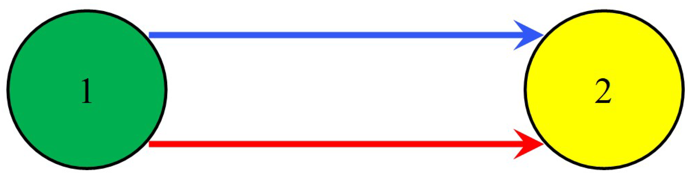
A network with a pair of nodes (Figure 1) is under study. There are two channels for transmitting information from the first node to the second node. The first channel has parameters ${\mu }_1$ and $N_1$, while $x_1$ units of information per second are delivered through them. The second channel has parameters ${\mu }_2$ and, similarly, $x_2$ units of information per second are delivered through them. It is necessary to increase the amount of information delivered by $\Delta x$ information units per second. One must determine which of the two channels should be increased in its load so that losses in the network are minimal.

To solve this problem in a general way, one should analyze three hypotheses:

-

the most efficient decision is to increase the channel load for which x is less, because it delivers less information;

-

the most efficient decision is to increase the channel load for which the loss probability is less, due to the assumption that it may have more free capacity than another;

-

the most efficient decision is to to increase the channel load for which $\mu -x$ is greater, since it has a larger bandwidth capacity.

Using this simple example, it is possible to show that solving the flow optimization problem, even in a simple network, is not always intuitive. It is worth considering the hypotheses one by one.

The first hypothesis is not true in general. Let us demonstrate it using the following example. Let network parameters be as follows: $x_1=2$ units of information/second, ${\mu }_1=1000$ units of information/second, $N_1=5$ and $x_2=1$ unit of information/second, ${\mu }_2=2$ units of information/second, $N_2=5$. According to the hypothesis, the first channel delivers twice as much information, so it is worth loading the second channel, although it is not correct, since its bandwidth capacity is too small.

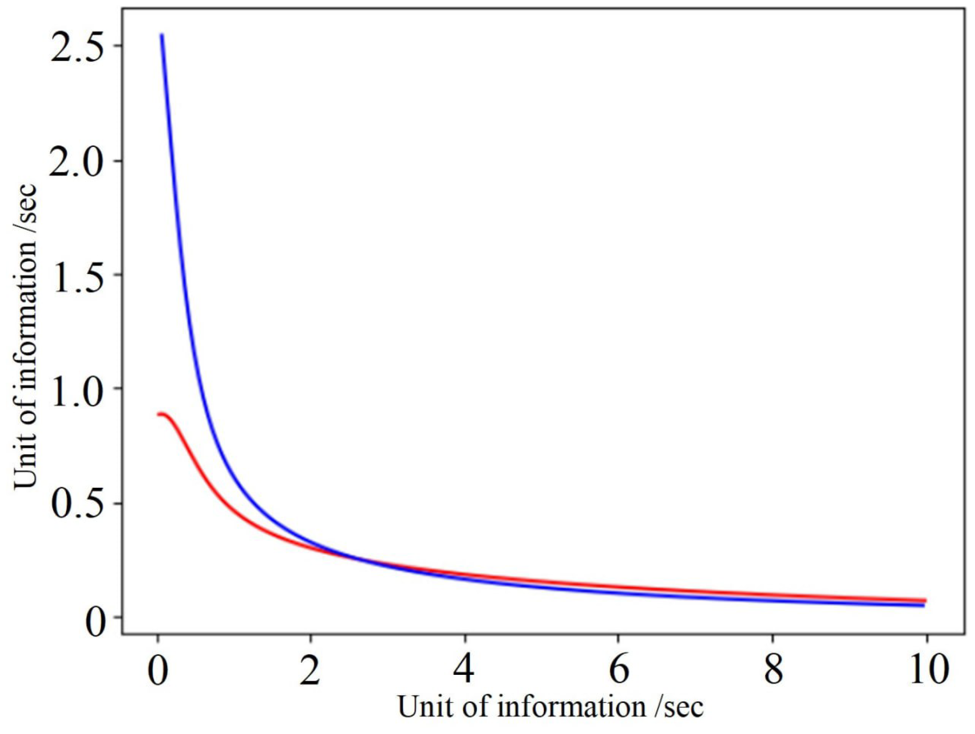
It is possible to prove that the second hypothesis is also wrong. Let us examine the graph in Figure 2. Axis X indicates the channel bandwidth capacity resource (information units/second), and axis Y indicates the change in the intensity of information loss (information units/second). In our calculations, the following network parameters are used: ${\mu }_1=30$ units of information/s, $N_1=3$ (blue curve in Figure 2) and ${\mu }_2=60$ units of information/sec., $N_2=9$ (red curve in Figure 2). The figure shows that when the useful information capacity resource reaches two units, it is preferable to load the second channel, and after four units it is preferable to load the first one. Therefore, it is impossible to determine which route is preferable for loading according to the remaining supply of useful information.

According to the third hypothesis, it is necessary to load the channel with a lower probability of losses. An example will demonstrate this. Let the first channel have the following parameters: ${\mu }_1=30$, $N_1=3$, and $x_1=13$. The parameters of the second channel are ${\mu }_2=60$, $N_2=9$, and $x_2=50$. The calculated loss probability in the first and second channels are $p_1=5.57\%$ and $p_2=5.25\%$, respectively. According to the third hypothesis, it is necessary to “load” the second channel, and the losses will be equal to $3.57$ units of information per second. However, when “loading” the first channel, the losses will be equal to $3.54$ units of information per second, i.e., it is better to use the first channel, even considering the higher probability of losses. Therefore, the third hypothesis is also wrong.

Thus, the use of obvious heuristics does not guarantee correct redistribution of information flows between two channels. However, it can be performed using derivatives evaluation of the information loss intensity function (8):

$$\frac{\partial E}{\partial x}=\underset{x\to 0}{lim}\frac{Loss(x+\Delta x)-Loss\left(x\right)}{\Delta x},$$

(8)

where $Loss\left(x\right)$ is the intensity of losses in the channel, under the condition that x units of information/sec. are delivered. The physical meaning of this value is as follows: it allows estimating the increased amount of information loss when adding an information flow, $\Delta x$ (units per second). In fact, the two streams are compared according to the criterion of minimum losses. This allows us to state the optimality of using the channel for which the derivative of losses in stream has the smallest value. This conclusion is of great importance and will be used further in this study. At the same time, finding the value of the function $Loss\left(x\right)$ in analytical form is impossible, so there is pseudo-code in the algorithm for finding $Loss\left(x\right)$ using the numerical method (Algorithm 3).

Algorithm 3 $Loss\left(Q\right)$

Required: $\mu$: channel bandwidth capacity, N: size of the channel buffer, Q: intensity of the information flow that must reach the output. Assign $k=0$. // iteration number Assign $e>0$. // stopping criterion Assign $p_{max}$. // second stopping criterion Assign $p^{\left(k\right)}=0$. // estimated probability of losses at the current iteration Start an endless loop: (a) Calculate $x^{\left(k\right)}=\frac{Q}{(1-p^{\left(k\right)})}$. // intensity of the information flow sent to the input (based on the estimated probability of losses) (b) Calculate $p^{(k+1)}=p(x^{\left(k\right)},\mu ,N)$. // real probability of losses at the current iteration (c) If $|p^{(k+1)}-p^{\left(k\right)}|<e$, then STOP and return the pair $\{flag=1;x_{rez}=x^{(k+1)}\}$. // the algorithm has converged, there is a solution (d) If $p^{(k+1)}>p_{max}$, then STOP and return the pair $\{flag=0;x_{rez}=None\}$. // the algorithm does not converge, and there is no solution (e) If none of the criteria are satisfied, then set $k=k+1$ and move on to the next iteration of the loop.

3.3. Estimating Partial Derivatives

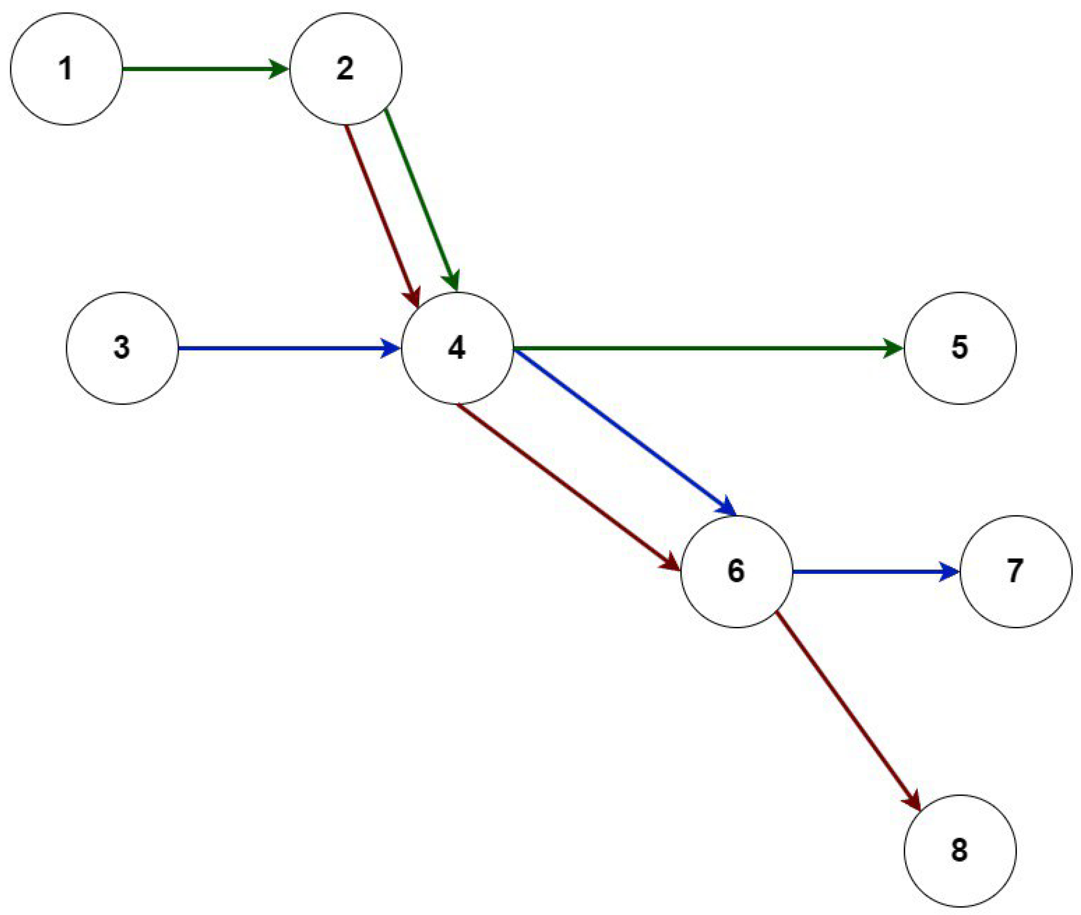
The dependence of variables on the probability of losses for the entire telecommunication network in accordance with changes of information flow at any edge of its graph by the value $\Delta x$ are under study. Let us consider the network shown in Figure 3.

The figure shows three routes connecting nodes: 1-2-4-5 (green arrows), 2-4-6-8 (brown arrows), 3-4-6-7 (blue arrows).

It is necessary to increase the data transfer rate for the information flow in the channel from the 6th node to the 7th by the amount $\Delta x_{67}$. It is obvious that the probability of $p_{67}$ loss has also increased. Since a certain amount of information is delivered along the route highlighted in blue (Figure 3), the incoming information flow to the 6th node must be increased by a certain amount, $\Delta x_{46}$, in order to compensate for the increase in the probability of information flow losses.

An increase in the channel load from the sixth node to the seventh node will lead to an increase in the load from the fourth node to the sixth node. Obviously, this, in turn, increases the load on the channel from the 3rd to the 4th nodes.

Analysis of the data shows that the load has increased along the entire route up to the seventh node, which is highlighted in blue. This leads to increased losses along the route highlighted in red in the channel from the fourth to the sixth node. These losses need to be compensated, so the load on the channel increases from the second node to the fourth node. Therefore, there are losses in the information flow along the route highlighted in green, which also need to be compensated.

In fact, since there are many more routes in a real network, and they intensively intersect with one another, a change in one channel load unpredictably increases the load in almost the entire network.

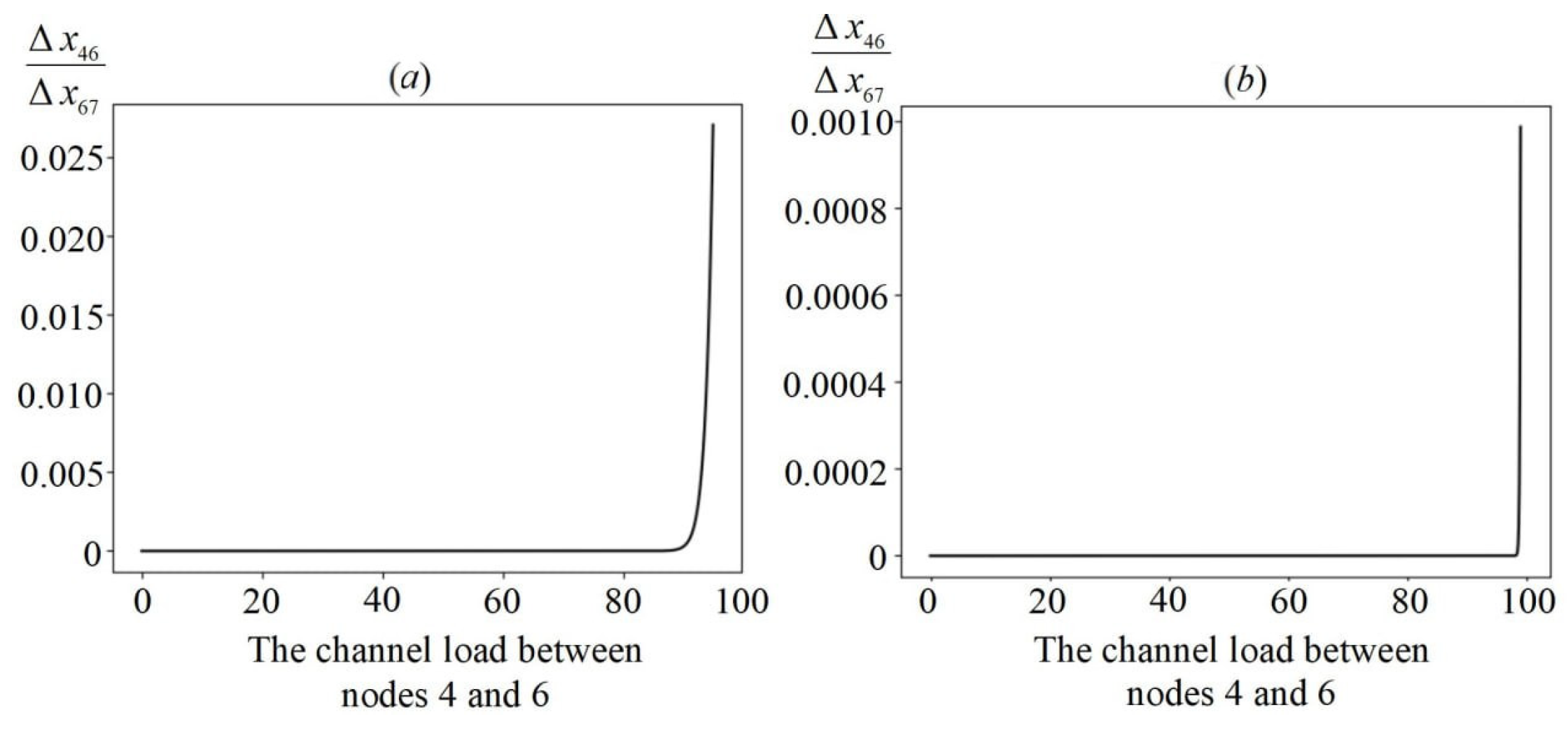
In practice, buffer sizes often start with 100–1000 packets. Figure 4a shows a graph of the relationship between changes in the intensity of information flows in channels between nodes 4 and 6 and 6 and 7 on the load of the channel between nodes 4 and 6. Figure 4b shows a similar graph, but with a buffer size of 1000 packets and a load of up to 99%. It can be seen that the amount of emerging additional information flows is no more than 2.5% of the main increase in $\Delta x$.

Therefore, the value of the derivative of the total information losses in the network with respect to the information flow in a particular channel only slightly exceeds the value of the derivative of the information losses in the channel with respect to the information flow in the same channel.

In other words, one can obtain the value of the derivative of the objective function by the information flow in the channel using the $Loss\left(Q\right)$ algorithm. Let the derivative value be marked as $\frac{\partial Loss}{\partial x_{ij}}$ for the corresponding channel from the ith node to the jth one.

Moreover, some modifications of Floyd’s algorithm (see Algorithm 4) make it possible to find a route with the best derivative value for each target request.

Algorithm 4 Modified Floyd algorithm

Required: the matrix of partial derivatives $dL=\left\{\frac{\partial Loss}{\partial x_{ij}}\right\}$, the loss probability matrix $p=\left\{p_{ij}\right\}$. Assign $d{L}_{ij}=\frac{d{L}_{ij}}{1-p_{ij}}\forall i,j$. For $i=\overline{1,n}$: (a) For $u=\overline{1,n}$: For $v=\overline{1,n}$: Assign $d_{new}=\frac{dL\left[u\right]\left[i\right]}{(1-p[u\left]\right[i\left]\right)}+dL\left[i\right]\left[v\right]$. // new distance if $d_{new}<dL\left[u\right]\left[v\right]$ then: // if the distance is better remember the new route Set $dL\left[u\right]\left[v\right]=d_{new}$, $p\left[u\right]\left[v\right]=p\left[u\right]\left[i\right]+p\left[i\right]\left[v\right]-p\left[u\right]\left[i\right]\times p\left[i\right]\left[v\right]$, $next\left[u\right]\left[v\right]=next\left[u\right]\left[i\right]$.

The result of executing Floyd’s algorithm is the matrix, which stores information about the shortest routes. Algorithm 5 allows obtaining route vectors in the form of a sequence of vertices.

3.4. Proposed Optimization Algorithm

The main idea of the optimization algorithm is to continue the coordinate descent along the promising directions found by the modified Floyd algorithm. We propose Algorithm 6 to determine the optimal distribution of traffic along the routes.

The computational efficiency of our approach is based on the limitation by a finite number of routes for each target request (there is no need to know all the routes). The validity of this assumption is demonstrated in the next section.

Algorithm 5 The shortest routes

Set the starting vertex u. Set the ending vertex v. Obtain the matrix of the shortest distances $dL$ by Floyd’s algorithm. Obtain the matrix of loss probabilities p by Floyd’s algorithm. If $p\left[u\right]\left[v\right]=1$ then STOP. // the route does not exist, stop the algorithm Assign $c=u$. Until $c\ne v$: (a) Add vertex c to the route. (b) $c=next\left[c\right]\left[v\right]$. Add vertex v to the route. STOP.

Algorithm 6 Optimization algorithm

Set $\Delta \omega =1$. // the step making changes in weights Set $k_{\omega }>1$. // in practice we use 1.015 Set $V=400$. // number of algorithm iterations Find the shortest routes using Floyd’s algorithm. Add the found route with weight $\Delta \omega$ to the archive of each target request. For $v=\overline{1,V}$: (a) Calculate network traffic loss $Calculate\text{\_}All\text{\_}Traffic$. (b) Find the shortest routes using modified Floyd’s algorithm. (c) $\Delta \omega *=k_{\omega }$. (d) For each target request: If the shortest route is already in the archive, then increase its weight by $\Delta \omega$. Otherwise, add the shortest route with weight $\Delta \omega$ to the archive. Generate a report

4. Computational Experiments

4.1. Stability of the Results

Local descent algorithms have a significant disadvantage. They converge to the nearest local optimum of the objective function. Therefore, it is necessary to investigate the extent to which the values of the resulting solutions depend on the starting points. For this reason, in the first iteration of the optimization algorithm random routes should be used, rather than the shortest ones.

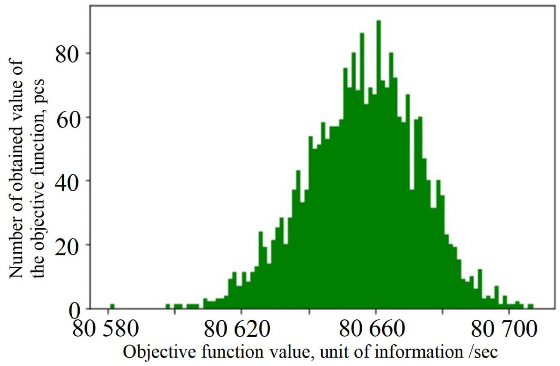
The developed algorithm was tested on data of a network consisting of 40 nodes and 2000 target requests. The network structure was fully connected. During the first iteration, a route consisting of approximately 25 nodes was added to the archive of each target request. Such a length of the route is sufficient, since the route length will not exceed 4 nodes in the optimal solution (if we discard unimportant routes). The starting routes can contain loops and channels with low bandwidth capacity.

Having carrying out 1000 numerical experiments on our algorithm with starting routes of random length, we obtained the results presented in the histogram (Figure 5).

From Figure 5, the diversity of values within the objective function is approximately 0.1% of its average value. When using the shortest starting routes, the value approaches the average obtained value of the objective function.

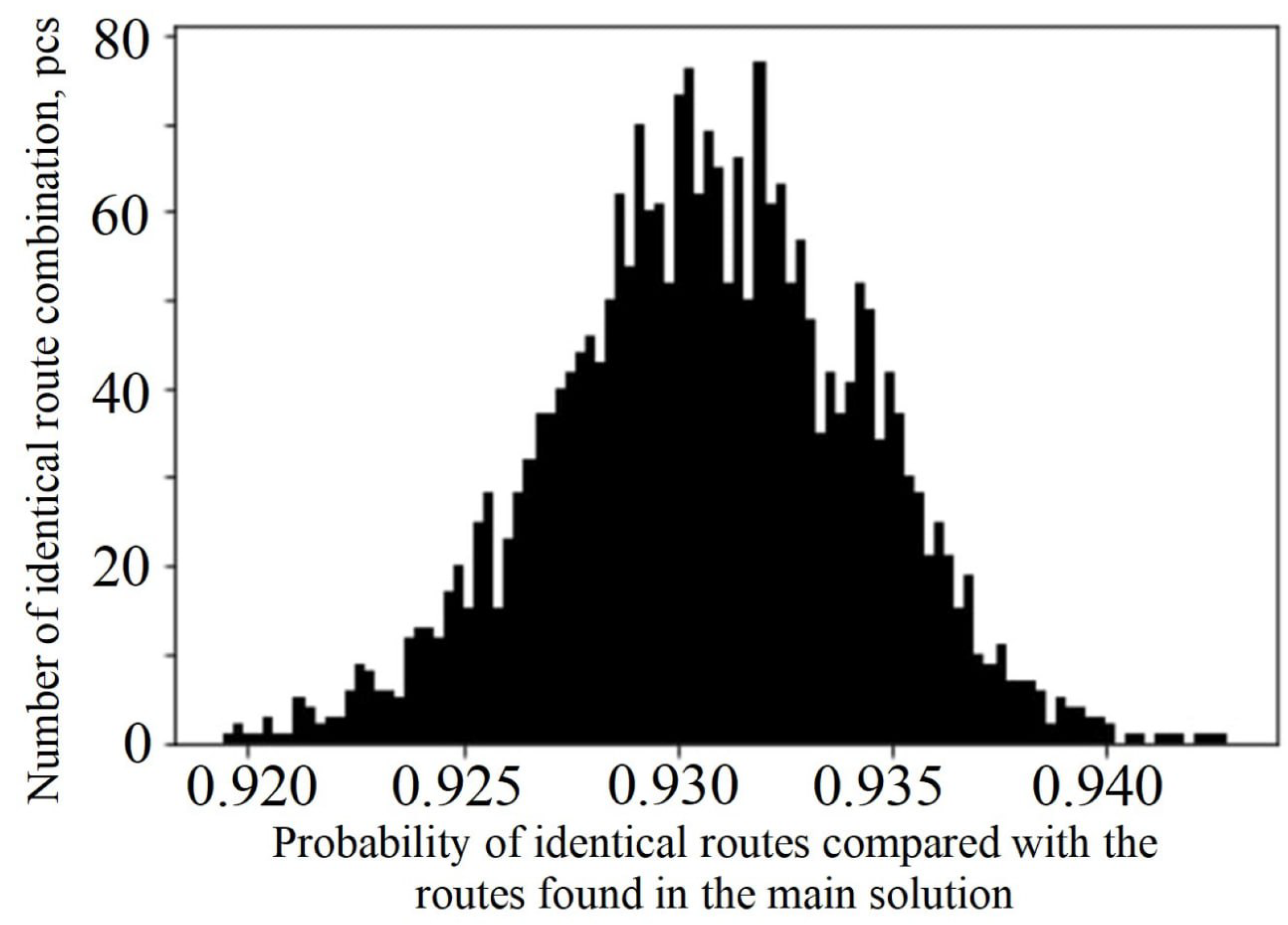
The objective function may have numerous local optima with similar values. For each solution, the part of ”important” routes located in the main solution is calculated. We define ”important” as a route transmitting more than 5% of all information of the target request. The distribution of the ratio of the matching routes is presented in Figure 6. It can be seen from the figure that the main solution, obtained with the shortest routes taken as the starting ones, forms 92–94% of the resulting solution. The slight difference in the compared routes can be explained by the fact that a small part of them in the framework of the algorithm may be defined as ”important” or as ”unimportant” routes. This is caused by data oscillations observed at the end of the algorithm and the fixed step of gradient descent.

It is important to mention that the optimization algorithm proposed in this work consists of two parts. The first is estimating derivatives (finding the gradient), and the second is finding the shortest routes using Floyd’s algorithm, which belongs to the category of greedy algorithms. Therefore, the proposed algorithm can be classified as a greedy-gradient algorithm.

4.2. Comparative Results

Let us compare the results of the developed optimization algorithm with those of the coordinate descent algorithm. Therefore, in both cases two test problems with arbitrary input parameters are used.

Test task #1, initial data:

-

number of nodes: 12;

-

number of target requests: 1000.

The value of the objective function obtained by the developed optimization algorithm is 37,606; the value of the objective function obtained by coordinate descent is 37,342, i.e., the difference is 0.702%.

Test task #2, initial data:

-

number of nodes: 40;

-

number of target requests: 2000.

The value of the objective function obtained by the developed optimization algorithm is 81,191; the value of the objective function obtained by coordinate descent is 80,768, i.e., the difference is 0.52%.

Since in the solutions obtained by the proposed optimization algorithm, the length of the optimal routes, did not exceed three nodes, all the routes with a length of no more than 4 nodes were used in the search space for the coordinate descent optimization algorithm. Therefore, the solutions obtained are quite close to optimal in terms in the value of the objective function, since additional optimization does not allow improvement of the value of the objective function by more than 1%. As coordinate descent frequently requires more calculations of the objective function, further complication of the optimization algorithm is of no use.

For low-dimensional problems (up to four nodes), the following algorithms were compared: the modified Gallagher’s method [20] and the greedy-gradient algorithm. The research results are presented in

Table 1. Comparative results of optimization algorithms.

Task No.	Number of Nodes	Number of Targeted Requests	Loss of Information
			Modified Gallagher’s Method	Greedy-Gradient Algorithm	The Coordinate Descent Algorithm in a New Search Space
1	4	12	6.85	6.84	-
2	4	12	308	308	-
3	4	12	11,762	9520	-
4	4	12	3 233	3237	-
5	4	12	23.08	23.08	-
6	4	12	9206	8154	-
7	12	1000	-	37,606	37,342
8	40	2000	-	81,191	80,768

.

When comparing the modified Gallagher’s method and the greedy-gradient algorithm, the network structure was unchanged, whereas the values of the target queries varied. The results obtained by these two algorithms either coincide with each other or differ significantly, which is explained by the multi-extremal nature of the objective function. At the same time, solving high-dimensional tasks using the modified Gallagher’s method is impractical, as the traditional optimization methods are not fast.

When solving large-dimensional problems (more than ten nodes), the following algorithms were compared: the greedy-gradient algorithm and the coordinate descent algorithm in a new search space. The results obtained using these two algorithms differ by no more than 1%.

For low-dimensional problems, with the use of the modified Gallagher’s method implemented in MATLAB, the calculation time does not exceed one minute on a commodity single-processor system. For the greedy-gradient algorithm implemented in the C++ programming language, the calculation time does not exceed 0.1 s using the same computer capability.

For high-dimensional problems, the calculation time of the greedy-gradient algorithm implemented in the same programming language, and with the same computer capability, does not exceed 10 s. For the coordinate descent algorithm in the new search space, implemented in the C++ programming language, using the same computer capability, the calculation time is does not exceed 30 h.

4.3. Efficiency of the Algorithm on Problems of Higher Dimension

Communication networks, including satellite ones, are becoming more complex. In this regard, the behavior of the prepositional algorithm and the time it takes for more cumbersome network topologies is interesting. Comparison with known methods in this case is difficult due to their unacceptable computational complexity. Therefore, in this subsection the behavior of the algorithm is studied depending on the complexity of the problems being solved.

For the experiments, a computer with the following characteristics was used: CPU Intel Core i5-12400F, RAM: DDR5, 32 GB, 4800 MHz, motherboard: Gigabyte B760M DS3H. Only one processor core was used.

The algorithm efficiency was estimated as follows: calculations for each version of the initial data were repeated 10 times and the results were averaged. The tested topologies were randomly generated with the following parameters: the number of nodes was 100, with an average of 20 edges outgoing from each node. Let us define the network density as the ratio of the number of outgoing edges to the number of nodes. In our case, the density was 0.2. The buffer size of each channel was 50. The number of target requests varied from 10 to 100 in steps of 10. The request intensity changed from 1 to 50 in steps of 0.1.

As a result, 4900 various data sets were generated. The entire modeling process can be divided into 10 parts; each part is characterized by a set of target queries from 10 to 100 in steps of 10. Thus, 490 experiments were generated within each part. All experiments can be divided into 2 parts: successful and unsuccessful. Successful experiments are those that resulted in the transfer of the entire planned amount of data required by the target requests. Each target request varied from 1 to 50 packets per second in steps of 0.1. The numbers of pairs of source and receiver nodes were randomly generated for each request.

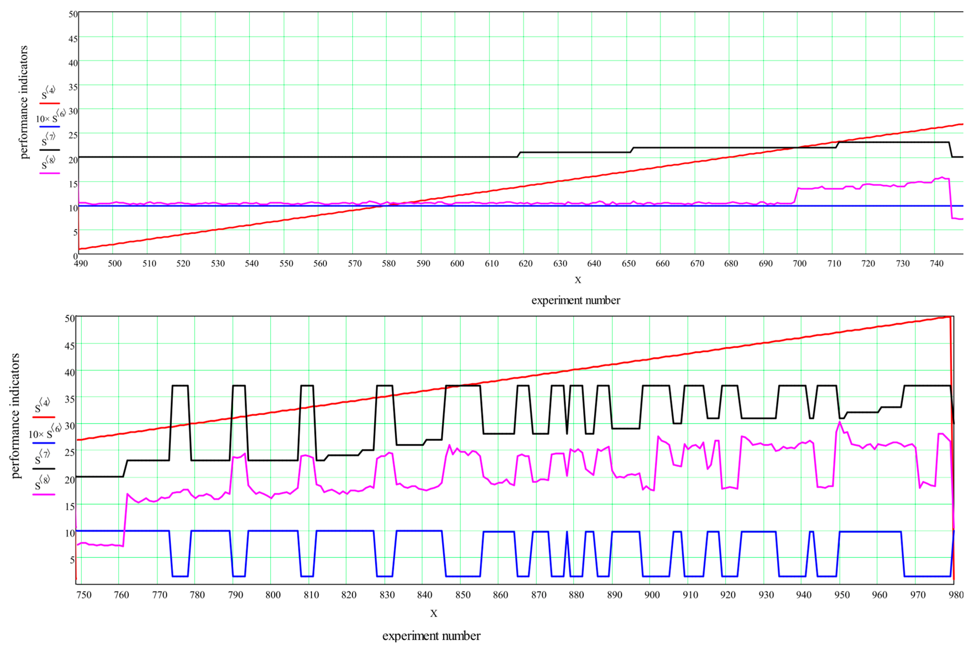
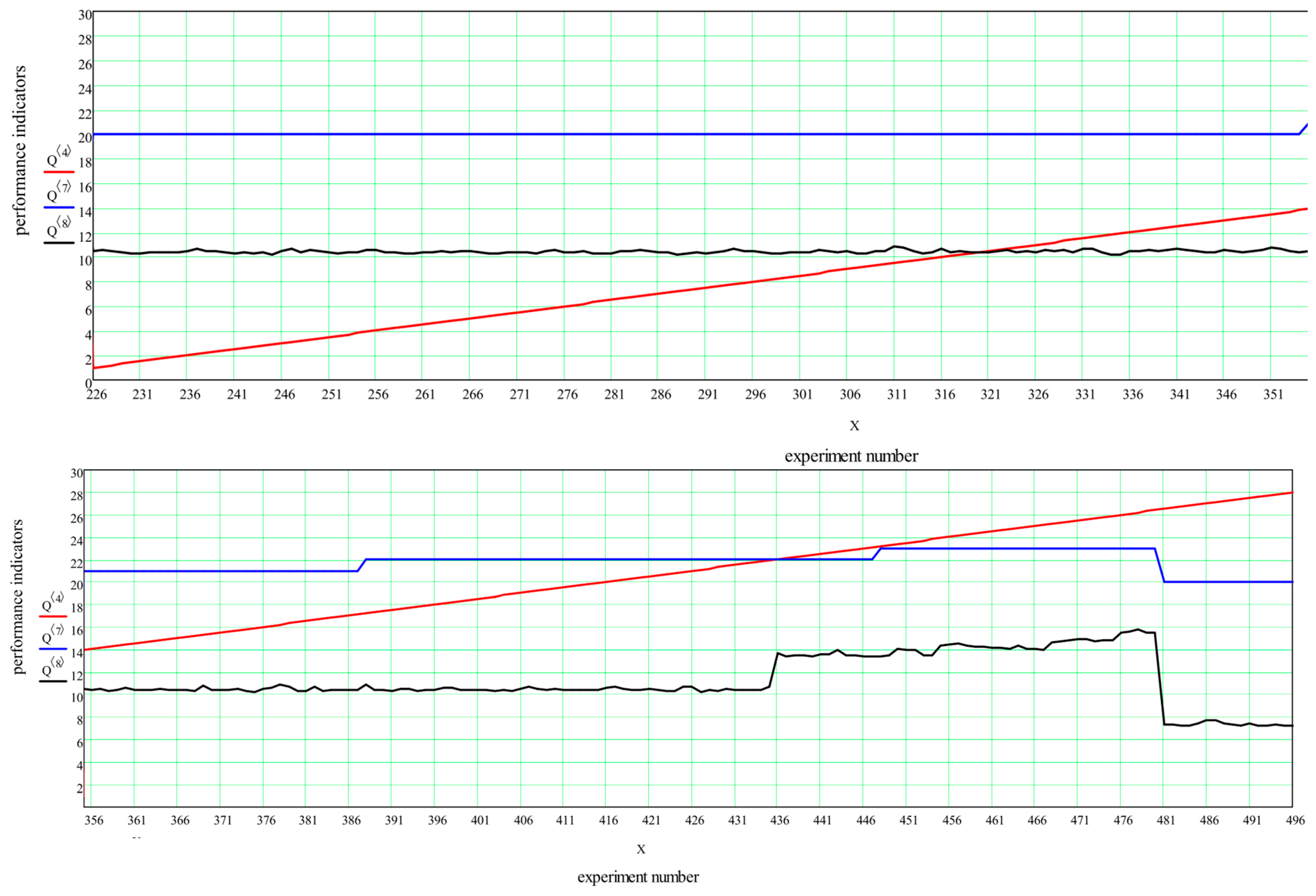
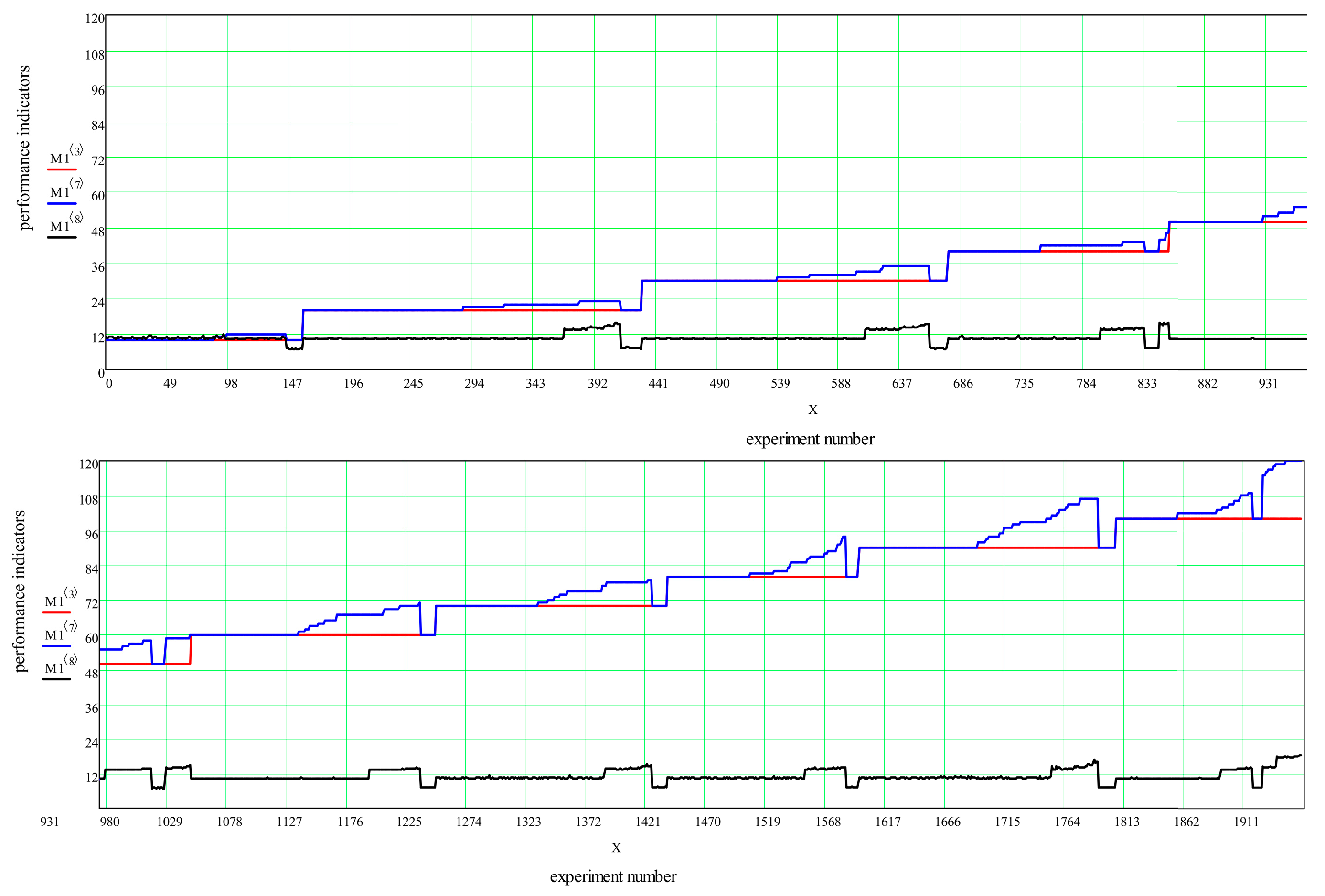
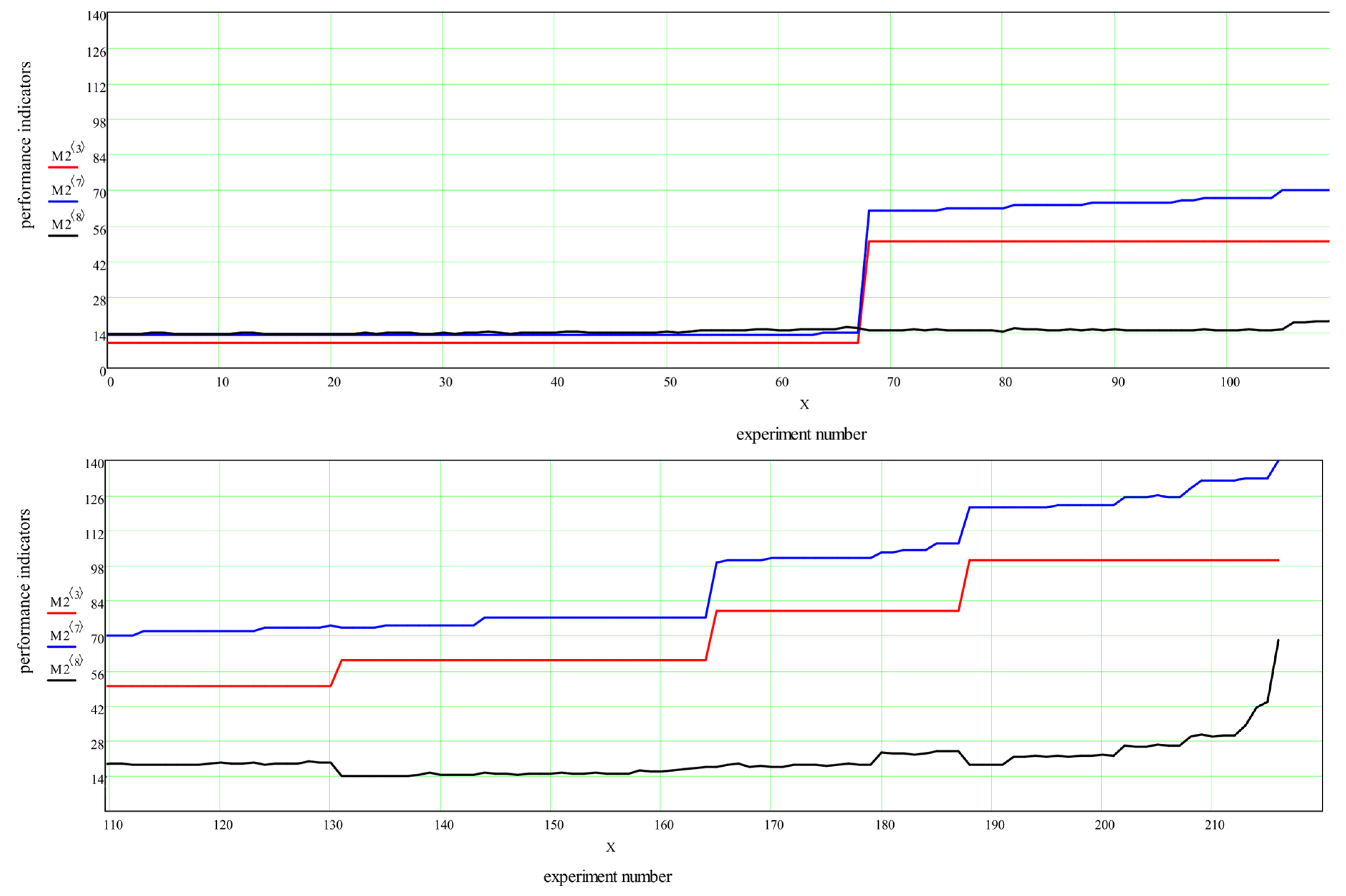
Figure 7 shows the second part, in which 20 requests were transmitted. As can be seen from the graphs, the execution time of the algorithm for finding the optimal distribution varies in proportion to the number of routes involved. An abrupt change in the number of routes corresponds to an abrupt change in the calculation time. It is also seen from Figure 8 that the maximum achievable request intensity is up to 28.1 packets per second. When it reaches a maximum of 50 packets/second during the experiment (Figure 7), this value corresponds to experiment 762 in Figure 7 and the extreme point.

Note that the maximum number of routes at which the possibility of transmitting all the data is granted does not exceed 23. This means that the generated topology and the selected sender and recipient nodes for each request are not selected in the most successful places in the topology. Since at least 20 routes are required to transmit data for 20 requests, in this case this means that only three additional routes were found, along which some of the requests managed to redistribute information flows. Figure 7 shows that with an increase in the intensity of requests, the algorithm managed to find 37 alternative routes for all requests. However, it was not possible to deliver all the required information to recipients, as can be seen after experiment 762.

Note that the criterion for stopping the algorithm was the objective function change at the next iteration not exceeding 10–8, if it finds a solution for transmitting all the traffic, or 40 iterations of the main algorithm if it is impossible to transmit the entire amount of information. Note that the authors followed certain goals for which this algorithm was developed, and these criteria for stopping were selected empirically for the problem being solved. Obviously, this criterion may not be suitable for all possible topological configurations and is the subject of further research.

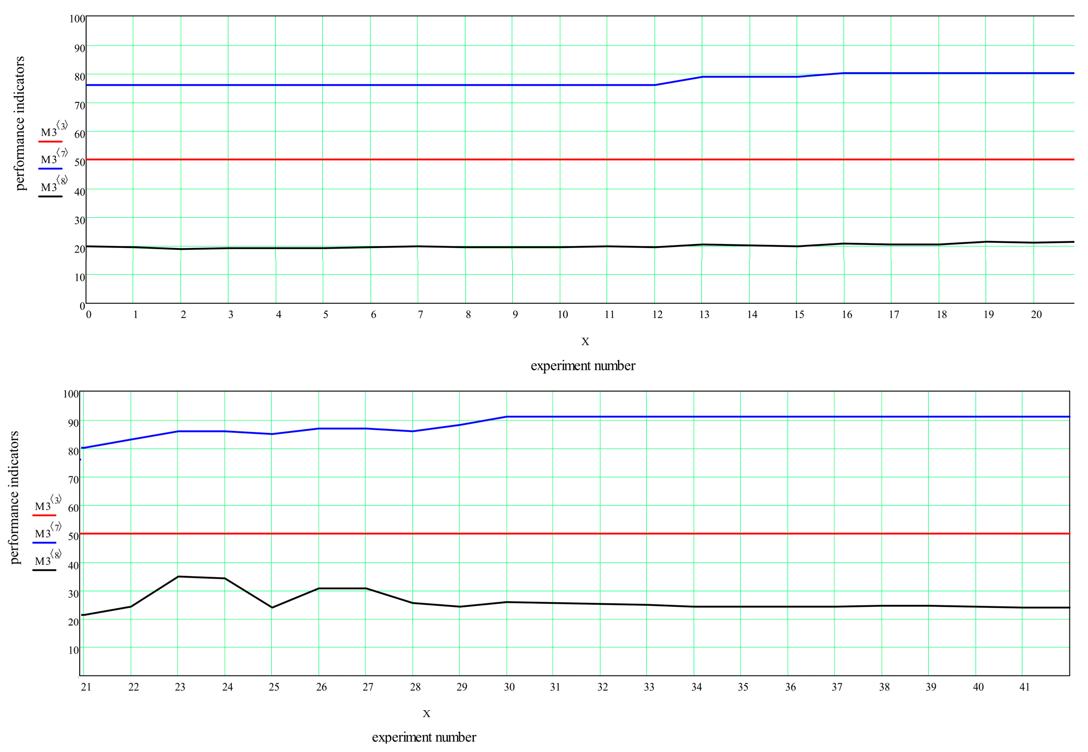
Let us analyze the average time for calculating the result for cases when it was possible to transmit all requests with the required intensity. We evaluated the algorithm performance in three modes. In the first mode, the ratio of the number of routes to the number of requests is in the range from 1 to 1.2 (Figure 9). The average running time of the algorithm for one experiment was 11.061 ms, the minimum time was 7 ms, and the maximum time was 18.5 ms. The number of experiments falling within this range was 1957.

In the second mode, the ratio of the number of routes to the number of requests was in the range from 1.2 to 1.5 (Figure 10). The average running time of the algorithm for one experiment was 17.236 ms, the minimum time was 13.3 ms, and the maximum time was 68.3 ms. The number of experiments falling within this range was 216.

In the third mode, the ratio of the number of routes to the number of requests exceeded 1.5 (Figure 11). The average operating time was 23.009 ms, the minimum time was 19 ms, and the maximum time was 34.8 ms. The number of such experiments was 42.

If we consider the worst of the results obtained before averaging for all 4900 experiments, for this experiment the algorithm execution time was 334 ms. In this experiment, a network was simulated in an overloaded state and the algorithm was unable to find the transmission routes for all the information. However, even this comparatively large amount of time is more than acceptable for modeling and control systems.

5. Conclusions

In this paper, we proposed a heuristic greedy-gradient route searching method to find the optimal distribution of traffic in telecommunication networks according to loss-minimizing criteria. This algorithm is capable of finding data transmission routes for the initial set of target requests and to distribute all network traffic among them according to the criterion of minimizing losses. To solve this problem, the Floyd–Warshall algorithm is used, in which the derivatives of the loss functions in the channel corresponding to each edge are used as the weights of the directed graph. Accordingly, the problem of traffic distribution along the resulting routes is solved.

The algorithm finds the same optimum regardless of the starting point of descent in the new search space. Despite the inaccuracies in calculating derivative estimates, the solution obtained is very close to the optimum in terms of the value of the objective function.

When solving high-dimensional test tasks, the developed algorithm is approximately 10,000 times faster than the coordinate descent algorithm in the new search space and at the same time corresponds to it in terms of the accuracy of the results obtained within 1%.

A feature of our new algorithm is the need to know the number of routes required to solve the optimization problem, which makes it similar to greedy algorithms and brings it closer in speed to them. On the other hand, computing pseudoderivatives to iteratively compute graph weights makes it akin to gradient algorithms. Another feature of this approach is that there is no need to explicitly compose the objective function and the constraints, as is required by streaming algorithms. In fact, the new algorithm solves a constrained optimization problem with a large number of equality-type constraints, which makes it difficult to solve by gradient methods. In the proposed approach, the constraints are taken into account when calculating the weight coefficients.

The considered example of modeling on a network of 100 nodes with a density of 0.2 demonstrates the capability of our new algorithm to simulate data transfer processes in real time, both during preliminary modeling and in communication network control systems. In this example, the largest number of target requests was equal to the number of nodes (each network node was assumed to be a source of information). Using mass-market computer equipment for such a network, the worst-case simulation took approximately 70 ms. The quality of the resulting solution ensured the delivery of all information. For overloaded networks, when it is impossible to find routes that ensure the delivery of all data the operating time of the algorithm did not exceed 340 ms, which is also quite acceptable.

In total, we carried out approximately 5000 experiments with the new algorithm, and the resulting time costs allow us to assert that the new algorithm is capable of effective modeling and control of any type of network due to the higher rate of operation of the algorithm compared to the rate of topology changes.

Our new algorithm is heuristic and does not guarantee the global optimality of the results. However, further research aimed at analyzing and clarifying the stopping criteria of the algorithm depending on the network structure seems to be promising and may further reduce the computation time. The use of the derivative of the loss probability function as a communication-channel metric in dynamic routing protocols depending on the state of the communication channel also seems promising, since preliminary experiments in this direction have shown good results.