Neural Network Based Approach to Recognition of Meteor Tracks in the Mini-EUSO Telescope Data

Abstract

Mini-EUSO is a wide-angle fluorescence telescope that registers ultraviolet (UV) radiation in the nocturnal atmosphere of Earth from the International Space Station. Meteors are among multiple phenomena that manifest themselves not only in the visible range but also in the UV. We present two simple artificial neural networks that allow for recognizing meteor signals in the Mini-EUSO data with high accuracy in terms of a binary classification problem. We expect that similar architectures can be effectively used for signal recognition in other fluorescence telescopes, regardless of the nature of the signal. Due to their simplicity, the networks can be implemented in onboard electronics of future orbital or balloon experiments.

1. Introduction

The JEM-EUSO (Joint Exploratory Missions for Extreme Universe Space Observatory) collaboration is developing a program of studying ultra-high energy cosmic rays (UHECRs) with a wide angle telescope from a low Earth orbit [1,2,3]. The idea is based on the possibility to register fluorescence and Cherenkov radiation in the ultraviolet (UV) range that is emitted during development of extensive air showers generated by primary particles hitting the atmosphere [4]. There are several benefits of this technique in comparison with ground-based experiments: (i) it can provide a huge exposure necessary for collecting sufficient statistics of these extremely rare events; (ii) the celestial sphere can be observed almost uniformly, which is important for anisotropy studies; and (iii) the whole sky can be observed with one instrument.

It became clear at early stages of the development of the JEM-EUSO program that an orbital telescope aimed at studying UHECRs can serve as a tool for exploring other phenomena that manifest themselves in the UV range in the nocturnal atmosphere of Earth [5]. It was demonstrated by TUS, the world’s first orbital fluorescence telescope aimed for testing the technique of studying UHECRs from space, that such an instrument can provide data on transient luminous events, thunderstorm activity, meteors, anthropogenic illumination of different kinds, and other types of signals [6,7]. In particular, observations of meteors are considered as an important branch of studies in the JEM-EUSO program [8,9].

The JEM-EUSO program is being implemented in a number of steps aimed at development and testing of different aspects of a full-blown orbital experiment. In particular, laser shots were successfully registered by a fluorescence telescope looking down on the atmosphere within the EUSO-Balloon mission [10]. A wide program of studies is being performed with the EUSO-TA experiment [11]. In 2018–2019, the Mini-EUSO (Multiwavelength Imaging New Instrument for the EUSO) telescope was built by the JEM-EUSO collaboration. It was brought to the International Space Station (ISS) on 22 August 2019, by the Soyuz MS-14 vehicle and has been operated since then as a part of an agreement between the Italian Space Agency (Agenzia Spaziale Italiana; ASI) and Roscosmos (Russia) [12,13,14,15]. The EUSO-SPB2 stratospheric balloon equipped with a fluorescence and Cherenkov telescopes made a short flight from Wanaka, New Zealand, in May 2023 [16,17,18]. All these instruments are aimed to be pathfinders and test beds for full-size orbital experiments like K-EUSO [19] and POEMMA [20].

Similar to the other projects of the JEM-EUSO collaboration, the Mini-EUSO telescope is registering multiple types of UV emission taking place in the nocturnal atmosphere of Earth, among them signals of meteors. A series of studies is dedicated to their search and analysis [21,22]. In the present paper, we continue our earlier research aimed at developing a method of recognizing meteor tracks in the Mini-EUSO data with neural networks [23]. A motivation for the study is the following. A conventional approach to finding signals of meteors in the Mini-EUSO data is time consuming and prone to numerous false positives. Thus, it is interesting to figure out if an approach based on machine learning (ML) and artificial neural networks (ANNs) can demonstrate higher efficacy than the conventional one so that both approaches complement each other. If so, it is interesting to test if results can be achieved with simple neural networks that can be implemented in the forthcoming orbital experiments, which are unlikely to have powerful onboard processors. These results can also be useful for recognizing tracks of extensive air showers in the future experiments since such signals resemble shapes and kinematics similar to those produced be meteors, though at completely different time scales. Finally, in case of the successful development of an ANN-based pipeline for recognizing meteor signals in the Mini-EUSO data, it can be applied for a search of track-like signals of different nature, including those that mimic extensive air showers. In what follows, we present a pipeline consisting of two basic neural networks that demonstrate high performance and can be trained on an ordinary PC. The work continues a series of studies fulfilled within the JEM-EUSO collaboration on application of machine learning and neural networks to analysis of data of fluorescence telescopes [24,25,26,27]. We do not present any results of applying the suggested method to data analysis since this will be covered in detail in a dedicated paper.

2. Mini-EUSO Experiment

The main components of the Mini-EUSO telescope include two Fresnel lenses and a focal surface (FS). The lenses have a diameter of 25 cm with the focal distance of the optical system equal to 300 mm. The FS has a square shape with 2304 pixels. It is built of 36 multi-anode photomultiplier tubes (MAPMTs) Hamamatsu R11265-M64 each consisting of $8\times 8$ pixels. All MAPMTs are grouped into nine so-called elementary cell (EC) units. Every EC unit has its own high-voltage system, which operates independently of the others providing necessary control of sensitivity of the respective MAPMTs. A 2-mm thick UV filter manufactured of the BG3 glass is located in front of each MAPMT. The size of one pixel equals $2.88\mathrm{mm}\times 2.88\mathrm{mm}$. The point spread function (PSF) has a size of ∼1.2 pixels. Mini-EUSO has a wide field of view (FoV) of ${44}^{\circ }\times {44}^{\circ }$ with spatial resolution (FoV of one pixel) equal to $6.3\mathrm{km}\times 6.3\mathrm{km}$. From the orbit of the ISS, an area observed by the telescope exceeds $300\mathrm{km}\times 300\mathrm{km}$. A detailed description of the instrument can be found in [12].

Mini-EUSO collects data in three modes. The D1 mode has a time resolution of 2.5 μs. This is called a D1 gate time unit (GTU). The D2 mode records data integrated over 128 D1 GTUs. Finally, the D3 mode operates with data integrated over $128\times 128$ D1 GTUs resulting in time resolution of 40.96 ms. To the contrary to the D1 and D2 modes, the D3 mode does not have a trigger, and its data can be considered as a series of videos with “seasons” corresponding to sessions of observations and “episodes” corresponding to night segments of the ISS orbit during a session. Each session takes around 12 h. With the orbital period of the ISS equal to 92.9 min, a typical session includes eight subsets of data taken during nocturnal segments of an orbit, with each of them taking slightly longer than 1/3 of the period. Every “video” has a resolution of $48\times 48$ pixels and consists of $T/40.96$ μs frames, where T is the duration of one nocturnal segment. Observations are performed approximately twice per month through the UV-transparent window at the Zvezda module with the schedule coordinated with other experiments. Due to this, background illumination varies strongly from one session to another depending on the phase of the Moon and the season. The D3 mode allows for registering meteors and other slow phenomena taking place in the night atmosphere of Earth. In what follows, we use only data recorded during sessions 5–8 and 11–14 taken from 19 November 2019 to 1 April 2020. All artificial neural networks discussed below were trained using data of seven sessions and tested on the remaining session. This way, we checked all possible combinations of the eight sessions.

3. Meteor and Background Signals

Signals of meteors registered with Mini-EUSO have some features important for the presented analysis:

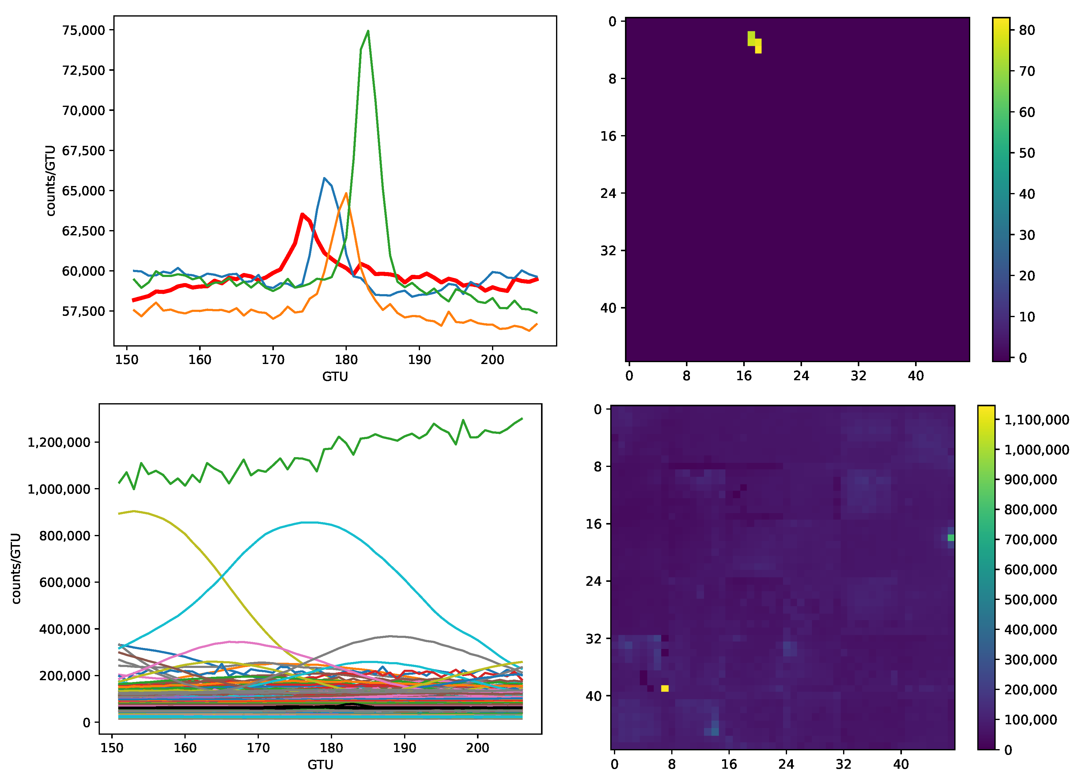
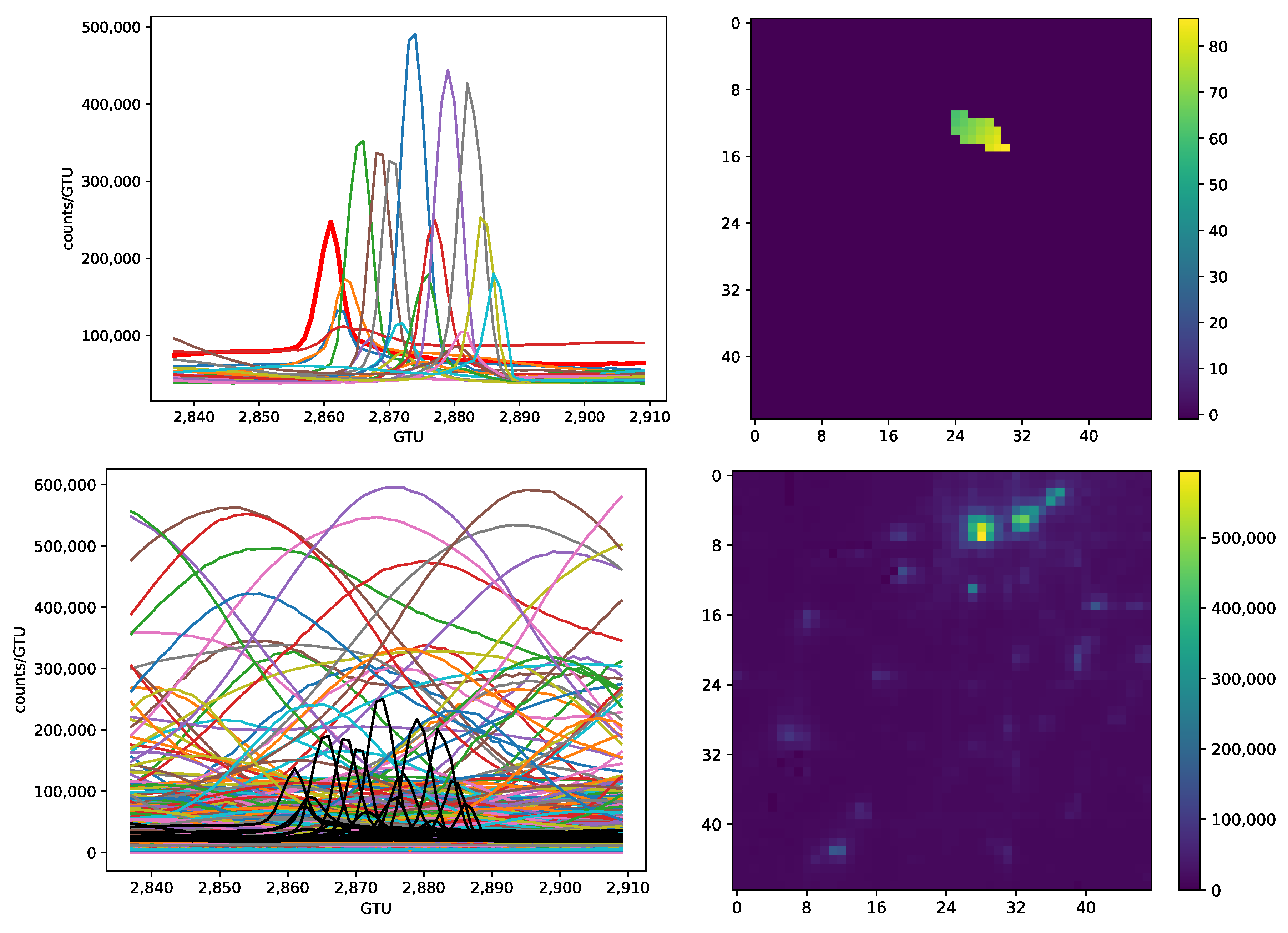
• A signal produced by a meteor in a pixel has a shape resembling the bell-like curve similar to the probability density function of the normal distribution.
• Meteor signals produce quasi-linear tracks in the focal surface.
• The number of hit (“active”) pixels in more than 75% of meteor tracks is ≤5, so that their footprints on the focal surface are small.
• Peaks of a meteor signal shift from one pixel to another (except for arrival directions close to nadir).
• There are multiple signals in the data with the shape similar to that of meteors but simultaneously illuminating large areas of the FS.
• Meteors are often registered on strong and quickly varying background illumination.
• The amplitude of a meteor signal is typically lower than amplitudes of some other signals in the FoV of Mini-EUSO registered simultaneously with the meteor.
• In some cases, it is impossible to judge unequivocally if a signal originated from a meteor or another source.

Let us discuss the most important of these features taking as an example signals demonstrated in Figure 1 and Figure 2.

Figure 1 provides an example of a bright and clearly pronounced meteor signal with numerous active pixels. The top row shows only the meteor signal, with the background illumination omitted. It can be seen that signals in every pixel have a typical shape resembling the bell curve (see the left panel). The peaks are shifted in time with respect to each other due to the meteor moving in the FoV of the instrument, resulting in a quasi-linear track on the focal surface (see the right panel). The task of recognizing meteor signals might look trivial after looking at these “pure” signals. However, the FoV of Mini-EUSO covers a huge area resulting in numerous different signals being registered simultaneously, with many of them being much brighter than those of meteors. This is demonstrated in the second row of Figure 1. The left panel shows shapes of all other signals recorded simultaneously with the meteor with the meteor signal shown in black. The right panel presents a snapshot of the FS made at the moment of the maximum of the meteor signal. The brightest pixel of the meteor has coordinates $(\mathrm{row},\mathrm{column})=(13,27)$ and can be seen as a small spot below a much brighter and extended area that appeared due to anthropogenic illumination (sine-like curves in the left panel). It is important to remark that the bottom rows of Figure 1 and Figure 2 demonstrate signals that were flat-fielded during an offline analysis for the sake of clarity.

However, all results presented below were obtained using raw data as they are recorded by the instrument. This was performed in order to understand how effectively is our method if implemented in onboard electronics.

An example of a typical meteor is shown in Figure 2. It has only four active pixels, and it is so dim in comparison with other illumination registered simultaneously that it is hardly possible to find it by eye in the bottom right panel presenting a snapshot of the focal surface at the moment of the maximum brightness of the meteor.

A conventional way to find meteor signals in the Mini-EUSO or TUS data would be to look for signals that can be fitted with the probability density function of a Gaussian distribution or its sum with a polynomial in case of non-stationary background illumination [21,22,28]. The known range of possible speeds of meteors (11–72 km s${}^{-1}$) together with information on the orbital speed of the ISS (∼7.7 km s${}^{-1}$), the FoV of one pixel, and the PSF size allows one to estimate the variance of a Gaussian fit. This also allows for verifying the kinematics of a signal moving across the FS. The latter step is of crucial importance since there are multiple signals in the Mini-EUSO data that can be fitted with a Gaussian distribution but take place simultaneously in big pixel groups without forming a track on the focal surface.

The task of recognizing meteor patterns in the Mini-EUSO dataset with machine learning methods can be considered as a binary classification problem since one basically needs to separate meteor signals from all the rest. Seemingly the most obvious way to tackle the task with artificial neural networks is to employ supervised learning. Within this approach, one can train an ANN using a labeled dataset. The dataset can be either prepared by simulations or extracted from real experimental data. It is tempting to choose the first way since meteor signals mostly have a bell curve shape similar to the density of the normal distribution. However, realistic simulations are not trivial since the background illumination is diverse, and sensitivity of different pixels on the FS is not known. This made us adopt the second approach.

We took two meteor datasets obtained by the JEM-EUSO collaboration and complemented them by our own analysis to prepare a dataset suitable for training and testing an ANN. It is necessary to stress once again that the source of a considerable number of bell curve-like signals registered with Mini-EUSO cannot be identified with confidence. Signals like those shown in Figure 1 and Figure 2 do not pose a problem in this respect. However, the shape and kinematics of tracks produced by meteors consisting of ≤4 pixels are often confusing. Another difficulty arises from dim signals on a strong and varying background. As a result, it is impossible to obtain ground-truth labels basing exclusively on the existing data set. After several tests, we confined the labeled dataset to signals the nature of which causes little doubt. In particular, we excluded almost all signals occupying two pixels. The resulting dataset used for training and testing ANNs discussed below consisted of 1068 meteor signals. Every record in the dataset included a timestamp of a meteor, coordinates of active pixels on the focal surface, and positions of the respective signal peaks.

Since data obtained in the D3 mode do not have a trigger but are similar to a series of videos each consisting of thousands of “frames” representing “snapshots” of the FS, there is a question how to extract samples containing meteor and non-meteor signals for training and testing datasets. For example, one can create data chunks of size $48\times 48\times T$, where T is the number of time frames (D3 GTUs) large enough to fit all meteors in the dataset and either center them on meteor peaks or put them in a fixed position with respect to the beginning of a meteor signal. This will allow one to obtain a “unified” representation of meteor signals to an ANN thus simplifying the task of their recognition. This way, non-meteor samples can be extracted from the rest of the data in a random fashion. However, this is not the way the data flow can be analyzed onboard. Besides this, the above approach will leave us with mere 1068 meteor samples, which is not sufficient to effectively train an ANN. This made us use a sliding window producing chunks that overlap by $dt$ GTUs. In what follows, we present results obtained for $dt=8$ GTUs that allowed us to avoid losing short meteor tracks and provided reasonable accuracy of their recognition. The procedure of labeling data chunks extracted this way will be explained in detail in Section 4.1.

We split the task of meteor signal recognition into two steps. First, we trained an ANN to recognize three-dimensional data chunks that contained meteor signals. After this, we employed another ANN to select pixels containing respective signals. Each ANN thus solved a task of binary classification. This allowed us to obtain lists of meteors registered with Mini-EUSO together with their active pixels thus providing information necessary for their subsequent analysis (reconstruction of brightness, arrival directions etc.).

4. Results

An important question to discuss before presenting ANNs is how to evaluate their performance. It is usually advised to use balanced datasets whenever possible, both for training and testing. In this case, the Receiver Operating Characteristic Area Under the Curve (ROC AUC) is one of the popular performance metrics [29]. Recall that the ROC curve is a plot of the true positive rate against the false positive rate at various threshold settings. Given one randomly selected positive instance and one randomly selected negative instance, AUC is the probability that the classifier will be able to tell which one is which. Due to its definition, ROC AUC does not depend on the sample size.

However, the number of meteor signals in the Mini-EUSO data is negligibly small in comparison with the number of non-meteor signals, so that using balanced datasets for testing would provide unrealistic results, while using them for training would not represent the full diversity of non-meteor signals thus resulting in lower performance and numerous false positives during tests. Thus, we unavoidably arrive at the necessity to use strongly imbalanced datasets both for training and testing. It is argued in the literature that ROC AUC does not act as a fully adequate performance metric in this case, and other metrics should be used instead, see, e.g., [30,31,32]. In what follows, we provide results obtained in terms of three more metrics besides ROC AUC. These are the Precision–Recall (PR) AUC, the Matthews correlation coefficient (MCC), and the $F_1$ score. One more metric will be introduced below.

Recall that the PR AUC equals an area under the plot of precision vs. recall with

$$\mathrm{Precision}=\frac{\mathrm{TP}}{\mathrm{TP}+\mathrm{FP}},\mathrm{Recall}=\mathrm{TPR}=\frac{\mathrm{TP}}{\mathrm{TP}+\mathrm{FN}},$$

where $\mathrm{TP}$, $\mathrm{FP}$, and $\mathrm{FN}$ are the number of true positives, false positives, and false negatives as classified by the model, respectively. The Matthews correlation coefficient can be calculated from the confusion matrix as

$$\mathrm{MCC}=\frac{\mathrm{TP}·\mathrm{TN}-\mathrm{FP}·\mathrm{FN}}{\sqrt{(\mathrm{TP}+\mathrm{FP})(\mathrm{TP}+\mathrm{FN})(\mathrm{TN}+\mathrm{FP})(\mathrm{TN}+\mathrm{FN})}},$$

where $\mathrm{TN}$ is the number of true negatives. Finally, the $F_1$ score is the harmonic mean of the precision and recall. It can be presented as

$$F_1=\frac{2\mathrm{TP}}{2\mathrm{TP}+\mathrm{FP}+\mathrm{FN}}.$$

Notice that these metrics will be applied to three-dimensional data chunks that partially overlap due to the employment of a sliding window for preparing input datasets. This can lead to a situation when a part of chunks containing a meteor signal are classified as non-meteor ones while others are classified properly, so that the value of a performance metric might be misleading. Since we are interested in maximizing the number of recognized meteors but not meteor chunks, it can be beneficial to also introduce a metric expressed in terms of the original 1068 meteors. Probably the most straightforward way is to use 1 − FNR (met), where FNR (met) is the false negative rate of meteor signals represented as the number of meteors lost by the classifier divided by the total number of meteors in a session used for testing.

All these metrics are equal to 1 for a perfect model. The MCC equals $-1$ for the worst possible model; other metrics give 0 in this case.

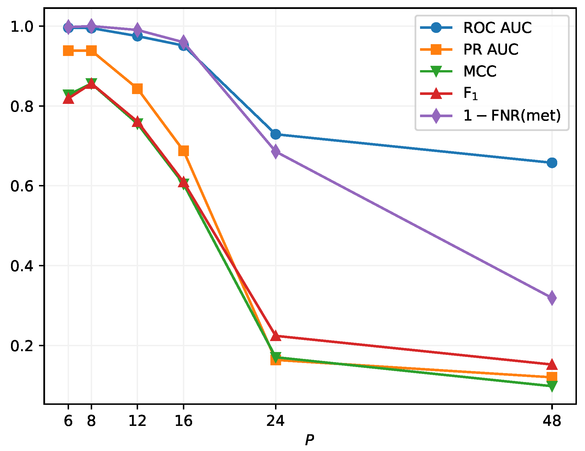
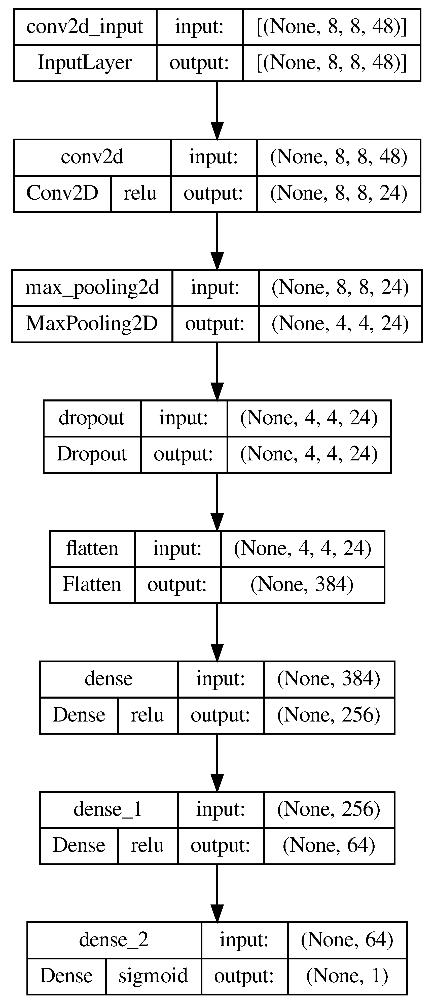
4.1. Recognition of Meteor Data Samples

One of the crucial questions to be solved before training an ANN is how to prepare and organize input data. In our case, the question is twofold. We need to decide how to label three-dimensional chunks into those that contain a signal of a meteor and those that do not. Besides this, we need to choose the size of data chunks $P\times P\times T$, where $P\times P$ defines the size of a square on the focal surface (measured in pixels), and T is the number of time frames (“snapshots” of the FS).

A data chunk was labeled as containing a meteor signal in case there were at least two meteor pixels inside a $P\times P$ area with peaks of the signals located within T GTUs. The reason is that we do not have a straightforward way to decide if a signal originates from a meteor with just a single active pixel. On the other hand, putting a more strict cut on the number of active pixels inside a chunk (≥3) results in a loss of short meteor tracks that have only two active pixels.

As for the number of time frames in data chunks, we tested $T=8,16,32,48,64$, and 128, which covers the range of duration of meteor signals in the dataset. Values $T=32$, 48, and 64 demonstrated the best results in our tests in terms of all metrics mentioned above with different combinations of training and testing sessions regardless of the value of P, with $T=48$ showing in average marginally better performance than the other two values. This value is used in all figures and tables presented below.

In [33], a simple convolutional neural network (CNN) was employed to perform binary classification of two types of signals registered with the TUS telescope. The instrument had a focal surface of $16\times 16$ pixels, and data arranged in $16\times 16\times T$ chunks worked well. Thus, we first tried training a CNN for Mini-EUSO with data chunks of the size $48\times 48\times T$. The input data was standardized according to the formula $(X_i-\langle X_i\rangle )/\sigma \left(X_i\right)$, where $X_i$ is the signal in pixel i, $\langle X_i\rangle$ and $\sigma \left(X_i\right)$ are estimations of the mean and the standard deviation during T time frames. However, as it was briefly reported in [23], this approach did not allow us to obtain acceptable results. We tested numerous configurations of CNNs and long short-term memory networks but failed to obtain ROC AUC $>0.75$ on testing datasets. A simple solution was found by splitting the FS into smaller squares. We tested splitting with $P=24,16,12,8$, and 6. In order to avoid losing signals around the boundaries of these small areas, we used overlapping by $P/2$ pixels in both directions. Figure 3 shows the behavior of mean values of different performance metrics for varying P with models trained on all possible combinations of seven sessions and tested on the remaining one. In this case, the same architecture of a CNN was used for all tests. It can be seen that performance expressed in terms of any metric increases quickly for $P<24$. The PR AUC, the MCC, and the $F_1$ score change in a very similar fashion while the values of the ROC AUC are close to those of $1-$ FNR (met) for small P. The best performance is reached for $P=8$ with the MCC and $F_1$ metrics slightly decreasing for $P=6$. Thus, data chunks of the size $8\times 8\times 48$ are used in what follows.

A CNN that we adopted for classifying meteor chunks consists of a convolutional layer with 24 filters and a kernel of size 3. It utilizes ReLU as an activation function and the L2 kernel regularizer with factor 0.1. The convolutional layer was followed by a maxpooling and dropout layers and two fully connected layers with 256 and then 64 neurons. Adam was used as an optimization algorithm. Sigmoid was employed as an activation function in the output layer. The architecture is shown in Figure 4.

The way we employed to prepare input data allowed us to obtain ≈18,000–24,000 thousand meteor chunks of the size $8\times 8\times 48$ depending on the set of sessions used for training, see details in

Table 1. The top row: sessions of observations used for testing CNNs trained on data of all other sessions. The second row: the total number of $8\times 8\times 48$ chunks (after augmentation) with signals of meteors used for training the respective CNNs. The number of original chunks is four times less. The last two rows: the number of chunks with meteor signals and the real number of meteors, respectively, in test sessions.

Test Session	5	6	7	8	11	12	13	14
Training meteor chunks	91,060	72,124	95,924	81,188	80,724	88,456	89,228	86,820
Testing meteor chunks	1712	6446	474	4180	4274	2341	2148	2772
Testing meteors	65	280	18	186	193	106	90	130

. These chunks were augmented then by the standard procedure of image rotation thus providing four times more samples. Non-meteor data chunks were selected in a random fashion, with their number being six times larger than the total number of meteor chunks (after augmentation). Twenty percent of the training dataset were used for validation during training. PR AUC was utilized as a performance metric during the training process. The loss function was defined as binary crossentropy. Validation loss was employed to adjust the learning rate and to avoid overfitting. Testing datasets included 100,000 non-meteor samples and all meteor data chunks available for the particular session varying from 474 chunks for session 7 up to 6446 chunks for session 6, see Table 1.

Table 2. Performance of the CNN on different sessions of observations. See the text for details.

Test Session	5	6	7	8	11	12	13	14
ROC AUC	0.992	0.994	0.999	0.993	0.994	0.998	0.993	0.996
PR AUC	0.937	0.955	0.876	0.933	0.946	0.973	0.931	0.956
MCC	0.872	0.894	0.732	0.857	0.888	0.921	0.782	0.901
F1	0.873	0.901	0.718	0.863	0.892	0.922	0.776	0.904
FNR (met)	0	0	0	0	0	0	0	0

contains values of five performance metrics described above for different combinations of testing and training datasets in the task of classification of $8\times 8\times 48$ chunks into meteor and non-meteor groups. For example, the column labeled as “5” presents results obtained with sessions 6–14 employed for training, and session 5 used for testing the CNN. It can be seen that zero out of 1068 meteors were lost in all sessions. Notice however that values of the PR AUC, the MCC, and the $F_1$ score vary considerably from one session to another.

4.2. Active Pixel Selection

At the second step, we want to separate pixels of 3-dimensional meteor chunks selected by the CNN into two groups: those containing the signal of a meteor (active pixels) and all the rest. Since meteor signals have a typical shape resembling the bell curve, as shown in the top left panels of Figure 1 and Figure 2, it is straightforward to train a multilayer perceptron (MLP) to solve the task. The input dataset consists of vectors of length $T=48$ now.

We followed the same way of training and testing the neural network as was used at the first stage. Namely, we trained an MLP on data extracted from seven sessions and tested it on the remaining one with all possible combinations of sessions. In order to avoid duplicate entries in the training dataset, we extracted data vectors from chunks of the size $48\times 48\times 48$. Due to a comparatively small shift $dt=8$ GTUs, we obtained samples with meteor signal peaks located at almost all possible positions along the time axis. The number of vectors (pixels) containing meteor signals in training data sets was up to 30 thousand, with non-meteor samples ten times greater. The input data was standardized similar to the CNN case. Twenty percent of training samples were utilized for validation. Binary crossentropy was used as the loss function and validation loss was employed to adjust the learning rate and to avoid overfitting. Testing was performed on all vectors extracted from meteor chunks of the size $8\times 8\times 48$ selected by the CNN. The number of chunks used for testing of each particular session data can be found in Table 1.

We compared a number of possible configurations of simple MLPs with one, two, and three hidden layers and different number of neurons. An optimizer, activation functions and a performance metric used for training were the same as for the CNN described above.

Table 3. Performance of the MLP on different sessions of observations. See the text for details.

Test Session	5	6	7	8	11	12	13	14
ROC AUC	0.992	0.995	0.993	0.994	0.996	0.993	0.995	0.995
PR AUC	0.899	0.932	0.877	0.916	0.932	0.887	0.936	0.928
MCC	0.790	0.841	0.744	0.826	0.847	0.812	0.809	0.835
F1	0.794	0.845	0.737	0.832	0.852	0.814	0.810	0.840
Mean IoU	0.808	0.853	0.773	0.843	0.861	0.829	0.825	0.850
FNR (pxl)	2/422	2/1428	0/80	7/928	5/958	0/492	0/457	2/630

presents results obtained with a two-layer MLP with 96 and 64 neurons in the two layers, respectively.

Similar to Table 2, Table 3 presents results illustrating performance of the MLP trained and tested on different sessions of data collection. Values of one more performance metric are shown here, namely, the mean values of the intersection-over-union (IoU) score. This function and its versions are often used in tasks of labeling pixels of images. It can be written as

$$\mathrm{IoU}=\frac{\mathrm{TP}}{\mathrm{TP}+\mathrm{FP}+\mathrm{FN}}.$$

It can be seen that values of the mean IoU metric are slightly above those of the $F_1$ score. The last line of the table shows the false negative rate calculated for pixels containing meteor signals. Two things can be easily noticed. First, the MLP did not properly recognize 18 out of 5395 active pixels, i.e., FNR (pxl) $\approx 0.33\%$. In this sense the accuracy can be estimated as 99.67% in average. On the other hand, the worst result was obtained for the test run on data from session 8 with FNR (pxl) $\approx 0.75\%$ so that the accuracy for this particular session equals 99.25%.

We have tried to address the same task with a few other machine learning methods, among them logistic regression, K nearest neighbors, the random forest, and XGBoost. We have failed to outperform results demonstrated with the MLP with any of them.

5. Discussion

We have demonstrated that a pipeline made of two simple neural networks, a CNN and an MLP, can be used to effectively recognize meteor tracks in the data of the Mini-EUSO fluorescence telescope that is observing the nocturnal atmosphere of Earth in the UV band from the International Space Station. The CNN used to select three-dimensional data chunks containing meteor signals managed to recognize properly all 1068 meteors in the dataset. The MLP employed to recognize pixels with meteor signals in data chunks picked up by the CNN, reached an accuracy beyond 99%. Neither of the ANNs puts high demands on computer resources necessary for their training. Besides this, they perform surprisingly fast during the classification stage with a major part of time being spent on reading data from a data storage, thus strongly outperforming the conventional algorithm.

We have seen in [33] that an ANN trained on data with clearly pronounced signals is able to identify patterns with low signal-to-noise ratio. Such events are classified as false positives during tests but their closer analysis reveals that their considerable part contains “positive” signals that were not found by the conventional algorithm used to prepare training and testing datasets. A preliminary analysis of signals marked as false positives in our tests has demonstrated that the same situation takes place with meteor tracks, so that the list of meteors can be extended with these newly found signals. The same applies to the list of active pixels. This is an important advantage of ML-based methods over conventional approaches.

One can anticipate that new experimental data might present new patterns of non-meteor signals since observational conditions vary strongly from one session to another. In this case, it might be necessary to extend the training dataset and retrain the ANNs. However, we do not expect that the architecture of the CNN and the MLP will need to be modified considerably. On the other hand, it is clear that the presented ANNs are not the only way of recognizing meteor tracks in the Mini-EUSO data using methods of machine learning. Still, it might be not easy to exceed the accuracy of the suggested pipeline with simple models. We plan to analyze other possible approaches, especially for the segmentation part. We are also going to address the task of solving the same problem in one step, without splitting it into two parts.

Finally, it is worth mentioning that the presented method is not confined to recognizing meteor tracks. Preliminary results of applying the same approach and even the same trained models for recognizing signals that mimic illumination expected from extensive air showers born by ultra-high energy cosmic rays, are quite promising and will be reported elsewhere. We also expect that this pipeline or a similar one can be implemented in onboard electronics of future orbital missions to act as a trigger for track-like signals of different nature manifesting themselves at various time scales.

References

1. Adams, J.H., Jr.; Ahmad, S.; Albert, J.N.; Allard, D.; Anchordoqui, L.; Andreev, V.; Anzalone, A.; Arai, Y.; Asano, K.; Ave Pernas, M.; et al. The JEM-EUSO instrument. Exp. Astron. 2015, 40, 19–44. [Google Scholar] [CrossRef]
2. Adams, J.H., Jr.; Ahmad, S.; Albert, J.N.; Allard, D.; Anchordoqui, L.; Andreev, V.; Anzalone, A.; Arai, Y.; Asano, K.; Ave Pernas, M.; et al. The JEM-EUSO mission: An introduction. Exp. Astron. 2015, 40, 3–17. [Google Scholar] [CrossRef]
3. Bertaina, M.E. An overview of the JEM-EUSO program and results. In Proceedings of the 37th International Cosmic Ray Conference—PoS(ICRC2021), Berlin, Germany, 15–22 July 2021; Volume 395, p. 406. [Google Scholar] [CrossRef]
4. Benson, R.; Linsley, J. Satellite observation of cosmic ray air showers. In Proceedings of the 17th International Cosmic Ray Conference, Paris, France, 13–25 July 1981; Volume 8, pp. 145–148. [Google Scholar]
5. Adams, J.H., Jr.; Ahmad, S.; Albert, J.N.; Allard, D.; Anchordoqui, L.; Andreev, V.; Anzalone, A.; Arai, Y.; Asano, K.; Ave Pernas, M.; et al. Science of atmospheric phenomena with JEM-EUSO. Exp. Astron. 2015, 40, 239–251. [Google Scholar] [CrossRef]
6. Klimov, P.A.; Panasyuk, M.I.; Khrenov, B.A.; Garipov, G.K.; Kalmykov, N.N.; Petrov, V.L.; Sharakin, S.A.; Shirokov, A.V.; Yashin, I.V.; Zotov, M.Y.; et al. The TUS Detector of Extreme Energy Cosmic Rays on Board the Lomonosov Satellite. Space Sci. Rev. 2017, 212, 1687–1703. [Google Scholar] [CrossRef]
7. Khrenov, B.A.; Klimov, P.A.; Panasyuk, M.I.; Sharakin, S.A.; Tkachev, L.G.; Zotov, M.Y.; Biktemerova, S.V.; Botvinko, A.A.; Chirskaya, N.P.; Eremeev, V.E.; et al. First results from the TUS orbital detector in the extensive air shower mode. J. Cosmol. Astropart. Phys. 2017, 9, 6. [Google Scholar] [CrossRef]
8. Adams, J.H., Jr.; Ahmad, S.; Albert, J.N.; Allard, D.; Anchordoqui, L.; Andreev, V.; Anzalone, A.; Arai, Y.; Asano, K.; Ave Pernas, M.; et al. JEM-EUSO: Meteor and nuclearite observations. Exp. Astron. 2015, 40, 253–279. [Google Scholar] [CrossRef]
9. Abdellaoui, G.; Abe, S.; Acheli, A.; Adams, J.; Ahmad, S.; Ahriche, A.; Albert, J.N.; Allard, D.; Alonso, G.; Anchordoqui, L.; et al. Meteor studies in the framework of the JEM-EUSO program. Planet. Space Sci. 2017, 143, 245–255. [Google Scholar] [CrossRef]
10. Adams, J.H.; Ahmad, S.; Allard, D.; Anzalone, A.; Bacholle, S.; Barrillon, P.; Bayer, J.; Bertaina, M.; Bisconti, F.; Blaksley, C.; et al. A Review of the EUSO-Balloon Pathfinder for the JEM-EUSO Program. Space Sci. Rev. 2022, 218, 3. [Google Scholar] [CrossRef]
11. Abdellaoui, G.; Abe, S.; Adams, J.; Ahriche, A.; Allard, D.; Allen, L.; Alonso, G.; Anchordoqui, L.; Anzalone, A.; Arai, Y.; et al. EUSO-TA—First results from a ground-based EUSO telescope. Astropart. Phys. 2018, 102, 98–111. [Google Scholar] [CrossRef]
12. Bacholle, S.; Barrillon, P.; Battisti, M.; Belov, A.; Bertaina, M.; Bisconti, F.; Blaksley, C.; Blin-Bondil, S.; Cafagna, F.; Cambiè, G.; et al. Mini-EUSO Mission to Study Earth UV Emissions on board the ISS. Astrophys. J. Suppl. Ser. 2021, 253, 36. [Google Scholar] [CrossRef]
13. Casolino, M.; Adams, J., Jr.; Anzalone, A.; Arnone, E.; Arnone, D.; Barghini, S.; Bartocci, M.; Battisti, R.; Bellotti, M.; Bertaina, F.; et al. The Mini-EUSO telescope on board the International Space Station: Launch and first results. In Proceedings of the 37th International Cosmic Ray Conference—PoS(ICRC2021), Berlin, Germany, 15–22 July 2021; Volume 395, p. 354. [Google Scholar] [CrossRef]
14. Marcelli, L.; Barghini, D.; Battisti, M.; Blaksley, C.; Blin, S.; Belov, A.; Bertaina, M.; Bianciotto, M.; Bisconti, F.; Bolmgren, K.; et al. Integration, qualification, and launch of the Mini-EUSO telescope on board the ISS. Rend. Lincei. Sci. Fis. Nat. 2023, 34, 23–35. [Google Scholar] [CrossRef]
15. Casolino, M.; Barghini, D.; Battisti, M.; Blaksley, C.; Belov, A.; Bertaina, M.; Bianciotto, M.; Bisconti, F.; Blin, S.; Bolmgren, K.; et al. Observation of night-time emissions of the Earth in the near UV range from the International Space Station with the Mini-EUSO detector. Remote Sens. Environ. 2023, 284, 113336. [Google Scholar] [CrossRef]
16. Scotti, V.; Osteria, G.; JEM-EUSO Collaboration. The EUSO-SPB2 mission. Nucl. Instrum. Methods Phys. Res. A 2020, 958, 162164. [Google Scholar] [CrossRef]
17. Cummings, A.; Eser, J.; Filippatos, G.; Olinto, A.V.; Venters, T.M.; Wiencke, L. EUSO-SPB2: A sub-orbital cosmic ray and neutrino multi-messenger pathfinder observatory. arXiv 2022, arXiv:2208.07466. [Google Scholar]
18. Eser, J.; Olinto, A.V.; Wiencke, L. Overview and First Results of EUSO-SPB2. In Proceedings of the 38th International Cosmic Ray Conference—PoS(ICRC2023), Nagoya, Japan, 26 July–3 August 2023; Volume 444, p. 397. [Google Scholar] [CrossRef]
19. Klimov, P.; Battisti, M.; Belov, A.; Bertaina, M.; Bianciotto, M.; Blin-Bondil, S.; Casolino, M.; Ebisuzaki, T.; Fenu, F.; Fuglesang, C.; et al. Status of the K-EUSO Orbital Detector of Ultra-High Energy Cosmic Rays. Universe 2022, 8, 88. [Google Scholar] [CrossRef]
20. POEMMA Collaboration; Olinto, A.V.; Krizmanic, J.; Adams, J.H.; Aloisio, R.; Anchordoqui, L.A.; Anzalone, A.; Bagheri, M.; Barghini, D.; Battisti, M.; et al. The POEMMA (Probe of Extreme Multi-Messenger Astrophysics) observatory. J. Cosmol. Astropart. Phys. 2021, 2021, 7. [Google Scholar] [CrossRef]
21. Barghini, D.; Battisti, M.; Belov, A.; Edoardo Bertaina, M.; Bisconti, F.; Capel, F.; Casolino, M.; Ebisuzaki, T.; Gardiol, D.; Klimov, P.; et al. Meteor detection from space with Mini-EUSO telescope. In Proceedings of the European Planetary Science Congress, EPSC2020–800, Online, 21 September–9 October 2020. [Google Scholar] [CrossRef]
22. Barghini, D.; Battisti, M.; Belov, A.; Bertaina, M.E.; Bertone, S.; Bisconti, F.; Capel, F.; Casolino, M.; Cellino, A.; Ebisuzaki, T.; et al. Analysis of meteors observed in the UV by the Mini-EUSO telescope onboard the International Space Station. In Proceedings of the European Planetary Science Congress, EPSC2021–243, Online, 13–24 September 2021. [Google Scholar] [CrossRef]
23. Zotov, M.; Sokolinskii, D. A Neural Network Approach for Selecting Track-like Events in Fluorescence Telescope Data. Bull. Rus. Acad. Sci. Phys. 2023, 87, 1054–1057. [Google Scholar] [CrossRef]
24. Vrábel, M.; Genci, J.; Bobik, P.; Bisconti, F. Machine Learning Approach for Air Shower Recognition in EUSO-SPB Data. In Proceedings of the 36th International Cosmic Ray Conference (ICRC2019), Madison, WI, USA, 24 July–1 August 2019; Volume 36, p. 456. [Google Scholar] [CrossRef]
25. Szakács, P.; Vrábel, M.; Genči, J. Classification of EUSO-SPB data using convolutional neural networks (CNNs). In Electrical Engineering and Informatics X, Proceedings of the Faculty of Electrical Engineering and Informatics of the Technical University of Košice; Technical University of Košice: Staré Mesto, Slovakia, 2019; pp. 262–267. [Google Scholar]
26. Filippatos, G.; Battisti, M.; Bertaina, M.E.; Bisconti, F.; Eser, J.; Osteria, G.; Sarazin, F.; Wiencke, L.; JEM-EUSO Collaboration. Expected Performance of the EUSO-SPB2 Fluorescence Telescope. In Proceedings of the 37th International Cosmic Ray Conference, Berlin, Germany, 15–22 July 2022; p. 405. [Google Scholar] [CrossRef]
27. Montanaro, A.; Ebisuzaki, T.; Bertaina, M. Stack-CNN algorithm: A new approach for the detection of space objects. J. Space Saf. Eng. 2022, 9, 72–82. [Google Scholar] [CrossRef]
28. Ruiz-Hernandez, O.I.; Sharakin, S.; Klimov, P.; Martínez-Bravo, O.M. Meteors observations by the orbital telescope TUS. Planet. Space Sci. 2022, 218, 105507. [Google Scholar] [CrossRef]
29. Fawcett, T. An introduction to ROC analysis. Pattern Recognit. Lett. 2006, 27, 861–874. [Google Scholar] [CrossRef]
30. Ferri, C.; Hernández-Orallo, J.; Modroiu, R. An experimental comparison of performance measures for classification. Pattern Recognit. Lett. 2009, 30, 27–38. [Google Scholar] [CrossRef]
31. Saito, T.; Rehmsmeier, M. The Precision-Recall Plot Is More Informative than the ROC Plot When Evaluating Binary Classifiers on Imbalanced Datasets. PLoS ONE 2015, 10, e0118432. [Google Scholar] [CrossRef] [PubMed]
32. Zhu, Q. On the performance of Matthews correlation coefficient (MCC) for imbalanced dataset. Pattern Recognit. Lett. 2020, 136, 71–80. [Google Scholar] [CrossRef]
33. Zotov, M. Application of Neural Networks to Classification of Data of the TUS Orbital Telescope. Universe 2021, 7, 221. [Google Scholar] [CrossRef]
34. Abadi, M.; Agarwal, A.; Barham, P.; Brevdo, E.; Chen, Z.; Citro, C.; Corrado, G.S.; Davis, A.; Dean, J.; Devin, M.; et al. TensorFlow: Large-Scale Machine Learning on Heterogeneous Systems. 2015. Available online: tensorflow.org (accessed on 30 April 2023).
35. Pedregosa, F.; Varoquaux, G.; Gramfort, A.; Michel, V.; Thirion, B.; Grisel, O.; Blondel, M.; Prettenhofer, P.; Weiss, R.; Dubourg, V.; et al. Scikit-learn: Machine Learning in Python. J. Mach. Learn. Res. 2011, 12, 2825–2830. [Google Scholar]
Figure 1. An example of a clearly pronounced meteor signal registered by Mini-EUSO on 20 October 2019. (Top left): signals in pixels that constitute the meteor signal. Signals in different pixels are shown in different colors. (Top right): location of meteor pixels in the focal surface. Colors denote time shift of the peaks with respect to the first one (in units of D3 GTUs). (Bottom left): all signals registered by Mini-EUSO simultaneously with the meteor. The black curves show the meteor signal. (Bottom right): a snapshot of the focal surface made at the moment of maximum of the brightest meteor pixel (GTU 2874).
Algorithms 16 00448 g001
Figure 2. A typical meteor signal registered by Mini-EUSO. (Top left): signals in pixels that constitute the meteor signal. (Top right): location of meteor pixels in the focal surface. Colors denote a time shift of the peaks with respect to the first one (in units of D3 GTUs). (Bottom left): all signals registered by Mini-EUSO simultaneously with the meteor. The black curves show the meteor signal. (Bottom right): a snapshot of the focal surface made at the moment of the brightest meteor signal (GTU 184).
Algorithms 16 00448 g002
Figure 3. Mean values of different performance metrics as a function of the data chunk size P for models trained on all possible combinations of seven sessions of observations and tested on the remaining session. See the text for details.
Algorithms 16 00448 g003
Figure 4. Architecture of the CNN used for binary classification in meteor and non-meteor data chunks. The total number of trainable parameters equals 125,465.
Algorithms 16 00448 g004