Design of a Lower Limb Exoskeleton: Robust Control, Simulation and Experimental Results

Abstract

This paper presents the development of a robust control algorithm to be applied in a knee and ankle joint exoskeleton designed for rehabilitation of flexion/extension movements. The goal of the control law is to follow the trajectory of a straight leg extension routine in a sitting position. This routine is commonly used to rehabilitate an injury on an Anterior Cruciate Ligament (ACL) and it is applied to the knee and ankle joints. Moreover, the paper presents the development and implementation of the robotic structure of the ankle joint to integrate it into an exoskeleton for gait rehabilitation. The development of the dynamic model and the implementation of the control algorithm in simulation and experimental tests are presented, showing that the proposed control guarantees the convergence of the tracking error.

1. Introduction

Robots can be classified by the functions they perform in cooperation with humans; however, in this article, only exoskeletons for rehabilitation are discussed. Exoskeletons are very useful in the rehabilitation of patients with motor deficiencies. Some examples of these include upper and lower limbs that are designed to guide movement, support weight, align body structures, protect joints, or correct deformities. Rehabilitation can be classified into the following:

• Passive rehabilitation: does not involve movement by the patient themself.
• Active rehabilitation: involves the participation of the patient, who is the one performing the movement.

The proposed prototype is intended to treat Anterior Cruciate Ligament (ACL) sprains and tears because they are the most common type of knee injury [1]. ACL injuries are more common in athletes who play high-demand sports like basketball, football, and soccer.

Ligament sprains are classified into:

• Sprains of Grade 1. They cause little ligament injury. Despite the fact that it has been considerably stretched, it could still aid in preserving the stability of the knee joint.
• Sprains of Grade 2. The ligament is stretched to the point of becoming loose. This is frequently referred to as a partial ligament tear.
• Sprains of Grade 3. This is a total ligament tear. The knee joint is unstable because the ligament has been split in half.

In [2], the authors presented some rehabilitation exercises for ACL injuries, which include movements of flexion/extension of the knee and ankle joints.

To develop rehabilitation exoskeletons, it is important to consider the analysis of movement of the biomechanics of the human being; for example, in [3], the main characteristics of the gait phases were determined to identify each gait phase. A long short-term memory-deep neural network (LSTM-DNN) algorithm was proposed for gate detection. There are a lot of prototypes used for rehabilitation, as in [4], where the exoskeleton was used for gait rehabilitation, or for patients with cerebral palsy as in [5].

In [6], the suggested robotic architecture considered the patients’ kinematic performance in addition to their psychophysiological condition, for example, heart and respiratory activity and galvanic skin response. Ref. [7] presented the development of assist-as-needed robotic rehabilitation. The main objective was to minimize robotic device intervention when following an established trajectory in order to promote patient engagement and improve training sessions.

It is very important that the prototype has the quality of being able to adjust to different patients, as in [8], where the authors discussed the lack of exoskeletons for minors, in particular the compatibility with children 6–11 years old. Ref. [9] presented a prototype that includes six degrees of freedom (DOF), divided into four for the lower limbs (two for knee joints and the other two for hip joints) and two for the system that permits standing and sitting activities. The exoskeleton was mechanically separated into two major components: the lifting system and the lower limb system, Figure 1 shows the exoskeleton prototype where we can observe that the joints corresponding to the ankles are missing.

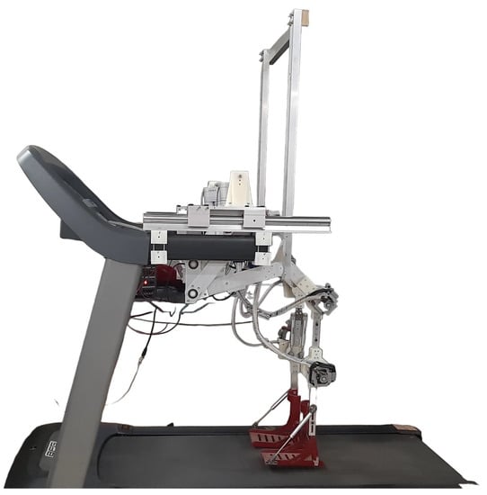
Figure 1. Exoskeleton for gait rehabilitation to assist in the task of standing–sitting the patient and the hip and knee movements [9].

The actuation system is one of the most important variables influencing the design of an exoskeleton since it impacts the general performance, efficiency, and portability [10]. Electrical motors, pneumatic actuators, hydraulic actuators, and elastic actuators are the most common types of actuators utilized in exoskeletons. Electric motors are used in most exoskeletons because they can be precisely regulated, and the energy source is easily available. However, some people prefer alternative choices because they have a greater power/weight ratio [11]. For example, in [12], the authors used hydraulic actuators, or other actuators as in review [13] where the prototypes employed different kinds of actuators such as servos, linear actuators, or a combination. There are also exoskeletons for active and passive rehabilitation of lower limbs, as in review [11]. The frame design is another significant feature of exoskeletons. Most exoskeletons have metal frames, and the most used is an aluminium alloy to connect the exoskeleton’s joints [14].

There are many options for control algorithms in exoskeletons, and the use of one of them depends on the desired benefits; it can be quick convergence or the smallest possible error. In particular, the robust control algorithm based on sliding mode type control laws has been implemented in different applications such as in [15], where it was used in a robotic vehicle, or in [16], where it was used in a robotic manipulator and in similar prototypes of exoskeletons as in [17], where good results can be seen. This algorithm is appropriate for our control problem due to the fast convergence despite the modelling uncertainty and the lack of knowledge of the parameters that change when the user changes, which are seen as disturbances.

In this paper, an exoskeleton was developed with rotary actuators to rehabilitate the knee and ankle joints. The proposed prototype is low-cost, lightweight, and easy to integrate into the exoskeleton in [9] to provide a greater range of motion. This will promote research to improve the prototype and use it for various applications in rehabilitation. This paper presents an exoskeleton prototype with four DOF divided into two DOF for knee joints and the other two DOF for ankle. The lower limb system is an anthropomorphic exoskeleton that supports the patient’s legs and feet and is powered by four motors whose axes correspond to the axes of rotation of the patient’s knee and ankle joints. The mechanical design of the prototype allows the exoskeleton to be customized for each patient. Finally, the exoskeleton contains a robust control based on a terminal high-order sliding mode control, which performs trajectory tracking. This control can achieve fast convergence in finite time of the states q and $\dot{q}$, have low tracking error and avoid the singularities that may cause an infinite input control.

2. Motion Analysis for Acl Injury Rehabilitation

In this section, the biomechanics of the ankle and knee joints are presented to obtain the trajectories of an ACL injury rehabilitation exercise.

2.1. Motion Required by the Prototype

The rehabilitation of an ACL injury includes flexion and extension of the knee and ankle joints. Flexion and extension movements are performed on the sagittal plane. As shown in Figure 2a for the knee joint and in Figure 2b for the ankle joint, the flexion occurs when the angle between the two segments that make up the joint decreases (acute angle), whereas extension occurs when the angle between the two segments of the joint increases (obtuse angle). The typical flexion–extension range for the ankle joint is ${75.6}^{\circ }$ [18], whereas the range of motion (ROM) for the knee joint is ${134}^{\circ }$ [19]. It is worth noting that the range of motion can vary considerably in each person [20]. Therefore, the movements that can be made by the prototype are flexion and extension of the joints. The minimum angle for the knee joint is $0^{\circ }$ and the maximum angle is ${110}^{\circ }$, and for the ankle joint, it is $0^{\circ }$ to ${65.1}^{\circ }$. Due to the fact that each person’s ROM is unique, the range of the prototype was reduced so that it could be used by everyone. As a result, the ROM of the prototype is lower than the real ROM of the joints. The ROM is described in Table 1.

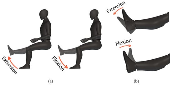
Figure 2. Biomechanics in the sagittal plane of the lower limb; (a) Flexion and extension movements for the knee joint; (b) Flexion and extension movements for the ankle joint.

Table 1. Range of motion for flexion and extension of the knee and ankle joints.

	ROM of the Human		ROM of the Robot
Joint	Minimum Angle	Maximum Angle	Minimum Angle	Maximum Angle
Knee	$0^{\circ }$	${134}^{\circ }$	$0^{\circ }$	${110}^{\circ }$
Ankle	$0^{\circ }$	${75.6}^{\circ }$	$0^{\circ }$	${65}^{\circ }$

2.2. Development of Trajectories of Motion

The desired trajectories $q_d$ or trajectories of motion were based on ACL injuries, so the trajectories proposed are for a straight leg extension routine in a sitting position, which is a combination of flexion and extension of the knee and ankle joints. The patient is in a sitting position during the rehabilitation process and undergoes a series of movements to improve the flexibility and strength of the lower limbs. To begin, the patient extends their knee joint and holds that position. Then, the patient stretches their ankle joint before returning it to its original position. The patient then moves their ankle joint into flexion before returning the knee joint to its original position, as shown in Figure 3.

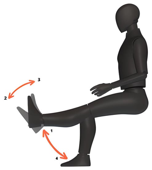
Figure 3. Straight leg extension routine in a sitting position; proposed routine for ACL injuries.

The desired trajectory of motion was captured using the OptiTrack motion capture system at 100 FPS in a healthy person who performed the routine. This technique uses a set of markers that are fixed to the item to track the motions of the object in its six degrees of freedom (distances and turns in X, Y, and Z). The system is based on a number of high-speed cameras that are calibrated and coordinated with one another and capture the motions of markers. The markers we utilized for this project were positioned on the knee and ankle joints, as well as the toe of the foot. Then, with the graphs of the position of the points of interest, we used the inverse kinematics of the modelled system in Figure 8 to obtain the trajectory of the angle position of the joints, knee $q_{d1}$ and ankle $q_{d2}$. Finally, we used a mathematical process to obtain the approximation of the trajectories.

Figure 4 shows the motion analysis laboratory where the motion trajectories were obtained.

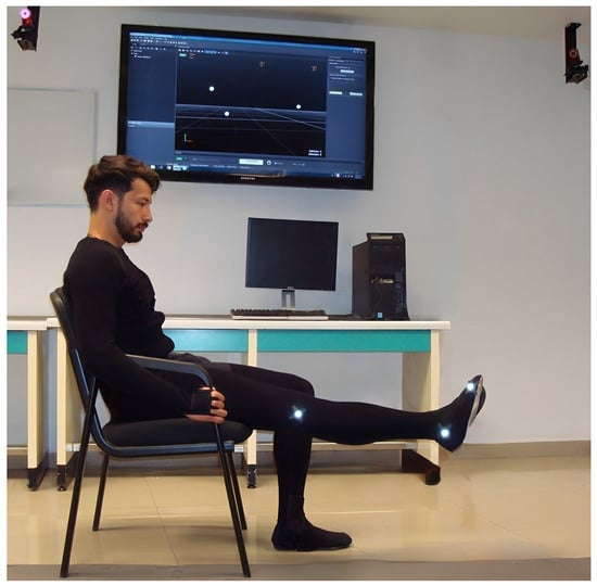
Figure 4. Motion capture system to obtain the desired trajectory or adequate rehabilitation routine, through a vision system with 12 cameras.

The trajectory for the knee joint is

$$\begin{array}{cc}\hfill & q_{d1}\left(t\right)=1.55[a_0+a_{1}cos\left(tw\right)+b_{1}sin\left(tw\right)+a_{2}cos\left(2tw\right)+b_{2}sin\left(2tw\right)\hfill \\ \hfill & +a_{3}cos\left(3tw\right)+b_{3}sin\left(3tw\right)+a_{4}cos\left(4tw\right)+b_{4}sin\left(4tw\right)\hfill \\ \hfill & +a_{5}cos\left(5tw\right)+b_{5}sin\left(5tw\right)+a_{6}cos\left(6tw\right)+b_{6}sin\left(6tw\right)\hfill \\ \hfill & +a_{7}cos\left(7tw\right)+b_{7}sin\left(7tw\right)+a_{8}cos\left(8tw\right)+b_{8}sin\left(8tw\right)]-100,\hfill \end{array}$$

where $a_0=37.42, a_1=-30.68,b_1=-8.15, a_2=-3.085,b_2=-3.583, a_3=3.041,$$b_3=2.28, a_4=0.01574, b_4=1.125, a_5=-0.7442, b_5=-0.1605, a_6=-0.4798,$$b_6=0.9625, a_7=0.2446, b_7=-0.2231, a_8=0.4532, b_8=-0.09683, w=0.35$, and for the ankle joint, it is

$$\begin{array}{cc}\hfill & q_{d2}\left(t\right)=-0.8[a_{00}+a_{01}cos\left(t{w}_0\right)+b_{01}sin\left(t{w}_0\right)+a_{02}cos\left(2t{w}_0\right)+b_{02}sin\left(2t{w}_0\right)\hfill \\ \hfill & +a_{03}cos\left(3t{w}_0\right)+b_{03}sin\left(3t{w}_0\right)+a_{04}cos\left(4t{w}_0\right)+b_{04}sin\left(4t{w}_0\right)\hfill \\ \hfill & +a_{05}cos\left(5t{w}_0\right)+b_{05}sin\left(5t{w}_0\right)+a_{06}cos\left(6t{w}_0\right)+b_{06}sin\left(6t{w}_0\right)\hfill \\ \hfill & +a_{07}cos\left(7t{w}_0\right)+b_{07}sin\left(7t{w}_0\right)+a_{08}cos\left(8t{w}_0\right)+b_{08}sin\left(8t{w}_0\right)]+54,\hfill \end{array}$$

where $a_{00}=70.89, a_{01}=-0.449, b_{01}=-4.386, a_{02}=-1.523, b_{02}=4.284, a_{03}=1.537,$$b_{03}=-7.771, a_{04}=-2.363, b_{04}=4.677, a_{05}=-0.0724, b_{05}=-2.737,$$a_{06}=-0.0426,$$b_{06}=1.991, a_{07}=-0.2973, b_{07}=-0.42, a_{08}=0.1964, b_{08}=0.1644,$$w_0=0.29$.

The real and approximated trajectories are shown in Figure 5.

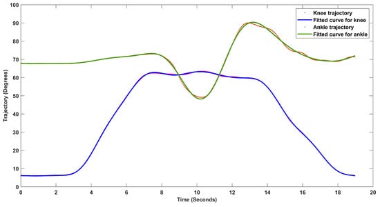
Figure 5. Motion trajectories for the knee $q_{d1}$ and ankle $q_{d2}$ joints when a straight leg extension routine in a sitting position type rehab routine is applied.

3. Mechanical Design of the Prototype

The objective of the mechanical design is to develop a prototype of the ankle joint to integrate it into the exoskeleton of six degrees of freedom of [9] to be able to use the exoskeleton in rehabilitation for ACL injuries. The developed lower limb exoskeleton considering the articulation of the knee and ankle was designed to meet the following requirements:

• Adjust the sizes to the Latin American population;
• Compact structure;
• Passive rehabilitation;
• Add mechanical stops to prevent hyperextension of the joints;
• The design must be ergonomic and easy to place.

The final design consists of two parts: the adjustment system for the calf length and the foot support. The exoskeleton rehabilitation movements are performed through a series of links attached by joints that correspond to the patient’s knee and ankle joints.

3.1. Ankle Joint Prototype

The prototype, shown in Figure 6, shows the mechanism made up of 36 pieces, without counting bolts, washers and nuts and was designed to allow easy adjustment to the calf and foot length of the patient; in this way, it can be used by a greater range of people with different heights and foot sizes.

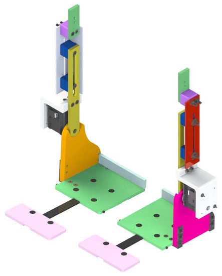
Figure 6. CAD design of the ankle rehabilitation exoskeleton that integrates with the gait rehabilitation exoskeleton.

The calf-length adjustment system subassembly was intended for simple calf-length adjustment on the patient. The smallest adjustment corresponds to a size of 40 cm, while the highest adjustment corresponds to a length of 48 cm. The foot support subassembly was developed to allow for easy modification of the patient’s foot length. The lowest adjustment for foot length is 17 cm, and the maximum adjustment is 27 cm. The minimum and maximum lengths are shown in Table 2.

Table 2. Maximum and minimum length of the prototype.

Dimension	Maximum	Minimum
Length of the calf	40 cm	48 cm
Length of the foot	17 cm	27 cm

It is very important to mention that for the safety of the patient, mechanical stops were added so that, in case of failures, the maximum range of movement allowed is not exceeded, the pieces in charge of this are the pink and the orange shown in Figure 6.

3.1.1. Stress Analysis

Stress analysis of the structure was performed to determine the materials and dimensions to be used for each part; we wanted the prototype to be lightweight and meet the previously established safety requirements. This analysis was performed in the SolidWorks program using its finite element tool. For material selection, aspects such as material availability, mechanical strength and weight were taken into account. After many tests, aluminium alloy was selected as the main material.

When designing a structure, it is desirable that the factor of safety be a number greater than one. This value indicates the ability of the system to exceed the requirements. The factor of safety is the ratio between the maximum power value of a system and the value to which it will be subject. The minimum factor of safety achieved for the prototype is 1.5.

3.1.2. Selection of the Motors

To select the actuator, it is necessary to know the maximum torque that it must provide; therefore, the following conditions were established:

• The axes of the actuators are aligned with the axes of the joints.
• The wearer does not apply muscular force.

Therefore, the required torque for the knee joint was provided by a harmonic drive motor FHA-14C-100-US200-E, which generates up to 20 Nm of torque. An absolute encoders model AMT203-V of the company CUI INC, Tualatin, USA, with a resolution of 12 bits and an SPI interface was used to measure the angular position of the link, and the angular speed and acceleration could be calculated. The torque for the ankle joint was provided by a Dynamixel MX-106T servomotor of the company ROBOTIS, which generates up to 5.6 Nm of torque. The angular position and the angular speed were obtained by the sensors included in it.

The motor for the ankle joint has special particularities. To control the actuator, it is necessary to convert its UART (Universal Asynchronous Receiver—Transmitter) signals to a half-duplex type and make the packages for sending and receiving data, which are expressed in a hexadecimal system.

3.2. Exoskeleton for Acl Injury Rehabilitation

Figure 7 shows the final exoskeleton prototype for rehabilitation, which includes the ankle joint prototype developed and integrated into the six DOF exoskeleton, now turning it into an eight DOF exoskeleton, divided into six for the lower limbs (two for the ankle, two for the knee joints and two for the hip joints) and two for the system that permits standing and sitting activities. Also, the prototype is complemented with an orthosis that provides greater comfort and fit for the patient when performing the routine.

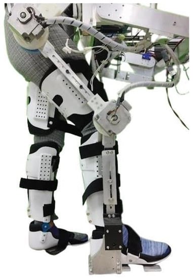
Figure 7. Developed prototype of a rehabilitation exoskeleton to assist the ankle and knee in ACL injury exercises.

4. Mathematical Model

In this section, we present the mathematical model of the prototype including the knee and ankle joints using the Euler–Lagrange formalism.

Dynamic Model

The exoskeleton is symmetrical, which means that the dynamic model is the same for both legs so the system can be reduced to a two DOF robot. In order to obtain the dynamic equations that govern the behaviour of the robot, it is necessary to have the simplified link diagram of the exoskeleton including the patient’s lower limb, which is presented in Figure 8, which shows the two links that make up the prototype, and there is a centre of mass for each one. The points (marked in red) are the joints and also the names that were assigned to each variable. The mass centre symbolizes the location where the system’s entire mass is supposed to be concentrated.

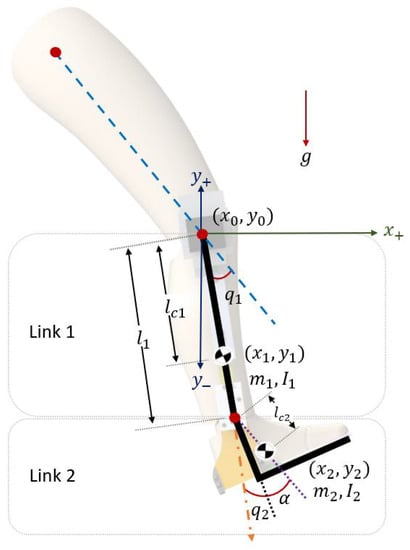
Figure 8. Simplified link diagram of the exoskeleton to develop the mathematical model.

The distances between the axis of rotation and the centre of mass of Link 1 and Link 2 are denoted by $l_{c1}$ and $l_{c2}$, while $I_1$ and $I_2$ express the moments of inertia of each link around the axis passing through their centres of mass. Both joints are rotational. The degree of freedom associated with angle $q_1$ is measured from the longitudinal axis of the thigh (line dotted in blue) to Link 1, which is positive in the counterclockwise direction, while $q_2$ is measured from the extension of the longitudinal axis through Link 1 to Link 2. Finally, $m_1$ and $m_2$ are the masses of the links. The position vector of the rotational joints with $q_1\left(t\right)$ corresponds to the knee joint and $q_2\left(t\right)$ for the ankle joint. The Euler–Lagrange formalism was used to obtain the dynamic model. The general equation of motion of the exoskeleton is

$$M\left(q\right)\ddot{q}+C(q,\dot{q})\dot{q}+g\left(q\right)=\tau$$

(1)

with

$$\left[\begin{array}{cc}{M}_{11}\left(q\right)& M_{12}\left(q\right)\\ M_{21}\left(q\right)& M_{22}\left(q\right)\end{array}\right]\left[\begin{array}{c}{\ddot{q}}_1\\ {\ddot{q}}_2\end{array}\right]+\left[\begin{array}{cc}{C}_{11}(q,\dot{q})& C_{12}(q,\dot{q})\\ C_{21}(q,\dot{q})& C_{22}(q,\dot{q})\end{array}\right]\left[\begin{array}{c}{\dot{q}}_1\\ {\dot{q}}_2\end{array}\right]+\left[\begin{array}{c}{g}_1\left(q\right)\\ g_2\left(q\right)\end{array}\right]=\left[\begin{array}{c}{\tau }_1\\ {\tau }_2\end{array}\right],$$

(2)

where $M\in R^{2x2}$ is the inertia matrix, $C\in R^{2x2}$ is the Coriolis matrix, $g\in R^2$ is the vector of gravitational forces and $\tau$$\in R^2$ are the torques of the actuators. Furthermore, the elements of the M, C and g matrixes are

$$\begin{array}{cc}\hfill M_{11}\left(q\right)& =I_1+I_2+m_2{l}_1^2+m_1{l}_{c1}^2+m_2{l}_{c2}^2+2m_2{l}_1{l}_{c2}\cos \left(q_2+\alpha \right),\hfill \\ \hfill M_{12}\left(q\right)& =I_2+m_2{l}_{c2}^2+m_2{l}_1{l}_{c2}\cos \left(q_2+\alpha \right),\hfill \\ \hfill M_{21}\left(q\right)& =I_2+m_2{l}_{c2}^2+m_2{l}_1{l}_{c2}\cos \left(q_2+\alpha \right),\hfill \\ \hfill M_{22}\left(q\right)& =I_2+m_2{l}_{c2}^2,\hfill \\ \hfill C_{11}(q,\dot{q})& =-m_2{l}_1{l}_{c2}\sin \left(q_2+\alpha \right){\dot{q}}_2,\hfill \\ \hfill C_{12}(q,\dot{q})& =-m_2{l}_1{l}_{c2}\sin \left(q_2+\alpha \right)\left[{\dot{q}}_1+{\dot{q}}_2\right],\hfill \\ \hfill C_{21}(q,\dot{q})& =m_2{l}_1{l}_{c2}\sin \left(q_2+\alpha \right){\dot{q}}_1,\hfill \\ \hfill C_{22}(q,\dot{q})& =0,\hfill \\ \hfill g_1\left(q\right)& =\left[m_1{l}_{c1}+m_2{l}_1\right]g\sin \left(q_1\right)+m_{2}g{l}_{c2}\sin \left(q_1+q_2+\alpha \right),\hfill \\ \hfill g_2\left(q\right)& =m_{2}g{l}_{c2}\sin \left(q_1+q_2+\alpha \right),\hfill \end{array}$$

(3)

and ${\tau }_1$ is the torque responsible for generating flexion and extension for the knee, while ${\tau }_2$ is the torque responsible for generating flexion and extension for the ankle.

5. Control Algorithm

Once the dynamics of the system are known, we proceed to propose a control algorithm that allows the prototype the following of a desired trajectory. For this reason, it takes into account that there are two actuators for the flexion–extension movements of the knee and the ankle. Then, the control law is designed so that $q_1$ and $q_2$ follow a desired path. It is proposed to apply a terminal high-order sliding mode control. The sliding mode control is robust to the uncertainties and unknown parameters, which are assumed to be bounded. This is useful for our application because the parameters such as $l_{c1},l_{c1},m_1$ or $m_2$ are different for each patient; the addition of the high order can reduce chattering. The prototype is designed for rehabilitation and it is desirable that it follows a smooth trajectory and the terminal part of the algorithm makes the tracking error converge to zero in finite time.

5.1. Control Algorithm

The following assumptions are made about the robot dynamics [21]:

$$\begin{array}{cc}\hfill & \parallel \mathrm{M}\left(\mathrm{q}\right)\parallel <{\alpha }_1,\hfill \\ \hfill & \parallel \mathrm{C}(\mathrm{q},\dot{\mathrm{q}})+\mathrm{g}\left(\mathrm{q}\right)\parallel <{\alpha }_3+{\alpha }_4\parallel \mathrm{q}\parallel +{\alpha }_2{\parallel \dot{\mathrm{q}}\parallel }^2,\hfill \\ \hfill & \parallel {\tau }_d\left(\mathrm{t}\right)\parallel <{\alpha }_5.\hfill \end{array}$$

(4)

The exoskeleton is subject to uncertainties in the parameters of the dynamic model. It is considered that the real values of the parameters are unknown. However, an estimate is available; therefore, the $M\left(q\right)$ matrix can be decomposed as

$$M\left(q\right)=M_e\left(q\right)+M_{\Delta }\left(q\right),$$

(5)

where $M_e\left(q\right)\in R^{nxn}$ contains the estimated parameters of the inertial matrix and $M_{\Delta }$$\left(q\right)$$\in R^{nxn}$ contains the unknown parameters. Therefore, Equation (1) can be rewritten as

$$M_e\left(q\right)\ddot{q}+M_{\Delta }\left(q\right)\ddot{q}=-C(q,\dot{q})\dot{q}-g\left(q\right)-\delta (q,\dot{q})+{\tau }_d+\tau .$$

(6)

Then, the angular acceleration is

$$\ddot{q}=M_e{\left(q\right)}^{-1}\tau -M_e{\left(q\right)}^{-1}[M_{\Delta }\left(q\right)\ddot{q}+C(q,\dot{q})\dot{q}+g\left(q\right)+\delta (q,\dot{q})-{\tau }_d].$$

(7)

By defining $F(q,\dot{q},\ddot{q})$, (7) becomes

$$\ddot{q}=M_e{\left(q\right)}^{-1}\tau -F(q,\dot{q},\ddot{q}),$$

(8)

where $F(q,\dot{q},\ddot{q})$ represents the unknown dynamics of the robot, shown in (9):

$$F(q,\dot{q},\ddot{q})=M_e{\left(q\right)}^{-1}[M_{\Delta }\left(q\right)\ddot{q}+C(q,\dot{q})\dot{q}+g\left(q\right)+\delta (q,\dot{q})-{\tau }_d].$$

(9)

We define the tracking error as

$$\begin{array}{cc}\hfill e& =q_d-q,\hfill \end{array}$$

(10)

$$\begin{array}{cc}\hfill \dot{e}& ={\dot{q}}_d-\dot{q},\hfill \end{array}$$

(11)

$$\begin{array}{cc}\hfill \ddot{e}& ={\ddot{q}}_d-\ddot{q}={\ddot{q}}_d-M_e^{-1}\left(q\right)\tau +F(q,\dot{q},\ddot{q}).\hfill \end{array}$$

(12)

Also, we assume that the unknown dynamics $F(q,\dot{q},\ddot{q})$ and its derivative $\dot{F}(q,\dot{q},\ddot{q})$ satisfy the following conditions:

$$\begin{array}{cc}\hfill \parallel F(q,\dot{q},\ddot{q})\parallel & \le {\Lambda }_1^T{B}_1,\hfill \\ \hfill \parallel \dot{F}(q,\dot{q},\ddot{q})\parallel & \le {\Lambda }_2^T{B}_2.\hfill \end{array}$$

(13)

Both are hypotheses used in the design of the control [16], where ${\Lambda }_1=[1\parallel q\parallel {∥\dot{q}∥}^2{]}^T$ and ${\Lambda }_2=[1\parallel \dot{q}{\parallel \cos \dot{\left|\right|q\left|\right|}]}^T$, while $B_1$ and $B_2\in {\mathbb{R}}^3$ are vectors with positive constant elements.

The proposed condition for $\parallel F(q,\dot{q},\ddot{q})\parallel$ is considering the sum of the individual assumptions in (4) of the matrices that make up the vector. For the sliding surface, the following variable is defined. Also, its derivative,

$$\begin{array}{cc}\hfill \sigma & =e+\Gamma {\int }_0^t{e}^{\left[v\right]}\left(\tau \right)d\tau ,\hfill \\ \hfill \dot{\sigma }& =\dot{e}+\Gamma e^{\left[v\right]},\hfill \end{array}$$

(14)

where $\sigma ={[{\sigma }_1,{\sigma }_2,\dots ,{\sigma }_n]}^T$, $e^{\left[v\right]}={\left|e\right|}^{v}sign\left(e\right)$, $0<v<1$ and $\Gamma \in R^{n\times n}$ is a positive diagonal matrix. The sliding surface is described as

$$\begin{array}{c}\hfill s=\ddot{e}+\beta \dot{\sigma }+\alpha \sigma ,\end{array}$$

(15)

where s represents the proposed surface vector, v is fractional order and $\alpha ,\beta >0$ are constant parameters. By substituting Equation (14) into (15),

$$\begin{array}{c}\hfill s={\ddot{q}}_d-M_e^{-1}\left(q\right)\tau +F(q,\dot{q},\ddot{q})+\beta (\dot{e}+\Gamma e^{\left[v\right]})+\alpha \left(e+\Gamma {\int }_0^t{e}^{\left[v\right]}\left(\tau \right)d\tau \right).\end{array}$$

(16)

The input control is defined as

$$\begin{array}{c}\hfill \tau =M_e[{\tau }_a+{\tau }_b],\end{array}$$

(17)

where ${\tau }_a$ is the input control for the known terms and ${\tau }_b$ is for compensating the unknown dynamics. Introducing Equation (17) into Equation (16),

$$\begin{array}{c}\hfill s={\ddot{q}}_d-{\tau }_a-{\tau }_b+F(q,\dot{q},\ddot{q})+\beta (\dot{e}+\Gamma e^{\left[v\right]})+\alpha \left(e+\Gamma {\int }_0^t{e}^{\left[v\right]}\left(\tau \right)d\tau \right).\end{array}$$

(18)

Therefore, the corresponding equation of ${\tau }_a$ is formulated as follows:

$$\begin{array}{c}\hfill {\tau }_a={\ddot{q}}_d+\beta (\dot{e}+\Gamma e^{\left[v\right]})+\alpha \left(e+\Gamma {\int }_0^t{e}^{\left[v\right]}\left(\tau \right)d\tau \right).\end{array}$$

(19)

Substituting Equation (19) into Equation (18),

$$\begin{array}{c}\hfill s=-{\tau }_b+F(q,\dot{q},\ddot{q}),\end{array}$$

(20)

Obtaining the derivative of Equation (20)

$$\begin{array}{c}\hfill \dot{s}=-{\dot{\tau }}_b+\dot{F}(q,\dot{q},\ddot{q}).\end{array}$$

(21)

5.2. Stability Analysis

We propose the candidate Lyapunov function as

$$\begin{array}{cc}\hfill V=& \frac{1}{2}{s}^{T}s,\hfill \end{array}$$

(22)

obtaining the derivative of V along the trajectories of the system.

$$\begin{array}{c}\hfill \dot{V}=s^T\dot{s}\end{array}$$

(23)

The control input ${\tau }_b$ is designed, which includes the sliding surface, to obtain a smooth control input. A low-pass filter is employed. Thus, ${\tau }_b$ is developed as follows:

$$\begin{array}{cc}\hfill & {\dot{\tau }}_b+c{\tau }_b=({\Lambda }_1^{T}P+{\Lambda }_2^T{B}_2)sign\left(s\right)+Ksign\left(s\right),\hfill \\ \hfill & {\Lambda }_1^{T}P\ge c{\Lambda }_1^T{B}_1,\hfill \end{array}$$

(24)

where $K=diag(k_1,k_2)$ is a positive diagonal matrix, P is a constant vector with positive elements and $c>0$.

Introducing Equations (13) and (24) into Equation (23),

$$\begin{array}{cc}\hfill \dot{V}=& -s^T({\Lambda }_1^{T}P+{\Lambda }_2^T{B}_2)sign\left(s\right)-s^{T}Ksign\left(s\right)+s^{T}c{\tau }_b+s^T{\Lambda }_2^T{B}_2.\hfill \end{array}$$

(25)

Constraining control input ${\tau }_b$ so that its absolute value is less than the bound of the unknown dynamics $F(q,\dot{q},\ddot{q})$, the inequality in Equation (24) can be rewritten as

$$\begin{array}{c}\hfill c|{\tau }_b|\le c{\Lambda }_1^T{B}_1\le {\Lambda }_1^{T}P.\end{array}$$

(26)

Applying Equation (26) in Equation (25),

$$\begin{array}{cc}\hfill \dot{V}\le & -s^T({\Lambda }_1^{T}P+{\Lambda }_2^T{B}_2)sign\left(s\right)-s^{T}Ksign\left(s\right)+s^T({\Lambda }_1^{T}P+{\Lambda }_2^T{B}_2)\hfill \\ \hfill \le & -\parallel s\parallel \parallel {\Lambda }_1^{T}P+{\Lambda }_2^T{B}_2\parallel -K\parallel s\parallel +\parallel s\parallel \parallel {\Lambda }_1^{T}P+{\Lambda }_2^T{B}_2\parallel .\hfill \end{array}$$

Thus, the above equation can be simplified as

$$\begin{array}{cc}\hfill \dot{V}\le & -K\parallel s\parallel ,\hfill \end{array}$$

(27)

and after performing some algebra, we obtain

$$\begin{array}{c}\hfill \dot{V}\le -K{V}^{1/2}.\end{array}$$

(28)

6. Results

6.1. Numerical Results

In this section, the simulation of the knee and ankle exoskeleton is presented by applying a terminal high-order sliding mode control algorithm, tracking the desired trajectory corresponding to a straight leg extension routine in a sitting position. The parameters of the exoskeleton used for the simulation are shown in Table 3.

Table 3. Properties of the prototype used in the numerical results.

Parameter	Variable	Value
Mass of the link 1	$m_1$	$0.25$ kg
Mass of Link 2	$m_2$	$0.793$ kg
Center of mass of Link 1	$l_{c1}$	$0.193$ m
Center of mass of Link 2	$l_{c2}$	$0.09$ m
Length of Link 1	$l_1$	$0.38$ m
Inertia of Link 1	$I_1$	$0.22$ kg · m ${}^2$
Inertia of Link 2	$I_2$	$0.32$ kg · m${}^2$
Alpha	$\alpha$	${9.6}^{\circ }$

The control algorithm is shown in Figure 9, where the first step is obtaining the tracking error (e) and its derivatives ($\dot{e}$ and $\ddot{e}$), then determining $e^v$ recalling that $e^v={\left|e\right|}^{v}sgn\left(e\right)$. After that, ${\tau }_a$ is calculated, which is the control law for the known dynamics, and then the sliding variable ($\sigma$) is obtained, and its derivative ($\dot{\sigma }$) is used to obtain the sliding surface (S), which is used to calculate ${\tau }_b$. Then, the total control input is generated that is provided to the dynamical model of the system.

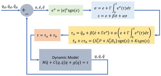
Figure 9. Block diagram of the exoskeleton robust control based on a terminal high-order sliding mode control.

The parameters used in the control are summarized in Table 4.

Table 4. Parameters used in the control.

Parameter	Variable	Value
Alpha	$\alpha$	$0.05$
Beta	$\beta$	20
Gamma	$\Gamma$	diag$(3,3)$
v	v	$0.1$
K	k	diag$(10,10)$
c	c	$0.5$
P	p	${\left[110.5\right]}^T$
$B_2$	$B_2$	${\left[115\right]}^T$

The initial conditions for the angular position and angular velocity are

$$\begin{array}{cc}\hfill & q\left(0\right)={[-90,0]}^T,\hfill \\ \hfill & \dot{q}\left(0\right)=0.\hfill \end{array}$$

The simulation results are shown in Figure 10 for the knee trajectory and in Figure 11 for the ankle joint, where the red dotted line is the desired trajectory for both cases, while the blue line corresponds to $q_1$ and the green one to $q_2$, which are the angular positions of the joints.

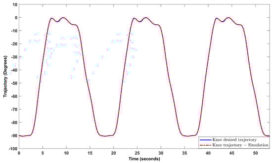
Figure 10. Trajectory tracking for the knee joint.

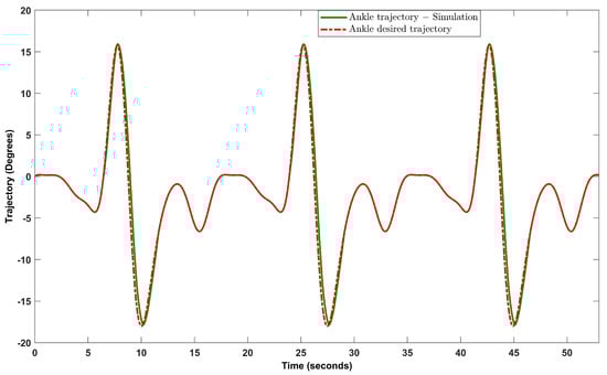
Figure 11. Trajectory tracking for the ankle joint.

It can be observed that both articulations follow their respective references.

Figure 12 shows the tracking error for the knee joint and Figure 13 shows that for the ankle joint, noting that the error in both cases tends to zero. The mean of the absolute error of the knee in the numeric simulation is ${0.0262}^{\circ }$, and for the ankle joint it is ${0.4477}^{\circ }$, while the standard deviation of the knee joint is ${0.0836}^{\circ }$, and for the ankle joint it is ${0.9917}^{\circ }$.

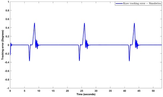
Figure 12. Tracking error obtained in the trajectory tracking for the knee joint.

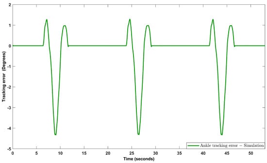
Figure 13. Tracking error obtained in the trajectory tracking for the ankle joint.

6.2. Experimental Results

After several experimental tests with different gains, the results of the routine for the knee and ankle joints for ACL injuries were obtained. The results shown are for three cycles of the proposed routine in Figure 5. However, the desired trajectories can also be modified so that the range of motion of the joints, as well as the duration of each cycle, can be adapted to the needs of each patient. For the experimental results, a duration of 19 s was defined for each cycle, and in total, the experimental test had a duration of 53 s.

The trajectories are shown in Figure 14 for the knee joint $q_1$ (blue line), and in Figure 15, they are shown for the ankle joint $q_2$ (green line), and the red line is the desired trajectory for both cases.

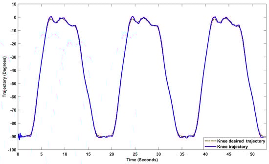
Figure 14. Trajectory tracking for the knee joint in real–time test.

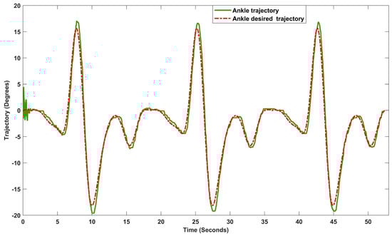
Figure 15. Trajectory tracking for the ankle joint in real–time test.

It can be observed that the two joints follow their respective references.

Figure 16 shows the tracking error for the knee joint and Figure 17 shows that for the ankle joint, noting that the error in both cases tends to zero. The mean of the absolute error of the knee in the experimental test is ${0.3236}^{\circ }$, and for the ankle joint it is ${0.6511}^{\circ }$, while the standard deviation of the knee joint is ${0.2628}^{\circ }$, and for the ankle joint, it is ${0.6431}^{\circ }$.

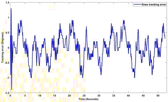
Figure 16. Tracking error obtained in the trajectory tracking for the knee joint in real–time test.

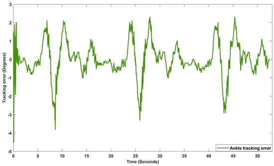
Figure 17. Tracking error obtained in the trajectory tracking for the ankle joint in real–time test.

7. Conclusions

In this paper, an exoskeleton was designed and manufactured to assist movements of flexion–extension of the knee and ankle joints for a passive rehabilitation of ACL injuries, for which it was necessary to know some topics related to medical robotics, as well as the biomechanics of the human body.

The prototype was designed considering the integration of an additional joint (ankle) to a previous exoskeleton and an effort study was carried out to determine the material and the dimensions to be used in order to carry the loads and be safe for the user. Therefore, it was possible to design and build a prototype with a lightweight design and resistance that can be altered to fit a variety of patients with different characteristics.

The design structure is capable of being integrated into the exoskeleton for gait rehabilitation in the UMI LAFMIA laboratory, making it possible to work on hip, knee, and ankle joints for flexion and extension.

The dynamic model that governs the movement of the robot was obtained considering the knee and ankle joints, which was developed from the Euler–Lagrange equations.

A robust control law based on terminal high-order sliding modes was proposed to study the behavior of the prototype when subject to an established trajectory; in the numerical results, the tracking errors converge to a bounded value close to zero.

Experimental tests were also carried out, demonstrating good performance of the exoskeleton when following the selected trajectories for both joints. Our primary objective was to achieve a smooth trajectory which is a highly desirable behavior in rehabilitation therapy. The mean errors observed in the experimental tests were ${0.3236}^{\circ }$ for the knee joint, and for the ankle joint, they were ${0.6511}^{\circ }$. Our proposed control method ensures convergence of the tracking error, even when the system is subjected to external perturbations during experimental tests.

The video of the experimental test can be accessed via https://youtu.be/ZATGTSApwgg (accessed on 18 September 2023) where the routine for ACL is performed.

References

- Larwa, J.; Stoy, C.; Chafetz, R.S.; Boniello, M.; Franklin, C. Stiff Landings, Core Stability, and Dynamic Knee Valgus: A Systematic Review on Documented Anterior Cruciate Ligament Ruptures in Male and Female Athletes. Int. J. Environ. Res. Public Health 2021, 18, 3826. [Google Scholar] [CrossRef] [PubMed]
- D’Isanto, T.; D’Elia, F.; Esposito, G.; Altavilla, G.; Raiola, G. Examining the Effects of Mirror Therapy on Psychological Readiness and Perception of Pain in ACL-Injured Female Football Players. J. Funct. Morphol. Kinesiol. 2022, 7, 113. [Google Scholar] [CrossRef] [PubMed]
- Zhen, T.; Yan, L.Y.P. Walking Gait Phase Detection Based on Acceleration Signals Using LSTM-DNN Algorithm. Algorithms 2019, 12, 253. [Google Scholar] [CrossRef]
- Tarnacka, B.; Korczyński, B.; Frasuńska, J. Impact of Robotic-Assisted Gait Training in Subacute Spinal Cord Injury Patients on Outcome Measure. Diagnostics 2023, 13, 1966. [Google Scholar] [CrossRef] [PubMed]
- Sarajchi, M.; Sirlantzis, K. Design and Control of a Single-Leg Exoskeleton with Gravity Compensation for Children with Unilateral Cerebral Palsy. Sensors 2023, 23, 6103. [Google Scholar] [CrossRef] [PubMed]
- Tamantini, C.; Cordella, F.; Lauretti, C.; Di Luzio, F.S.; Campagnola, B.; Cricenti, L.; Bravi, M.; Bressi, F.; Draicchio, F.; Sterzi, S.; et al. Tailoring upper-limb robot-aided orthopedic rehabilitation on patients’ psychophysiological state. IEEE Trans. Neural Syst. Rehabil. Eng. 2023, 31, 3297–3306. [Google Scholar] [CrossRef] [PubMed]
- Pezeshki, L.; Sadeghian, H.; Keshmiri, M.; Chen, X.; Haddadin, S. Cooperative Assist-as-Needed Control for Robotic Rehabilitation: A Two-Player Game Approach. IEEE Robot. Autom. Lett. 2023, 8, 2852–2859. [Google Scholar] [CrossRef]
- Goo, A.C.; Wiebrecht, J.J.; Wajda, D.A.; Sawicki, J.T. Human Factors Assessment of a Novel Pediatric Lower-Limb Exoskeleton. Robotics 2023, 12, 26. [Google Scholar] [CrossRef]
- Rosales-Luengas, Y.; Espinosa-Espejel, K.I.; Lopéz-Gutiérrez, R.; Salazar, S.; Lozano, R. Lower Limb Exoskeleton for Rehabilitation with Flexible Joints and Movement Routines Commanded by Electromyography and Baropodometry Sensors. Sensors 2023, 23, 5252. [Google Scholar] [CrossRef] [PubMed]
- Huo, W.; Mohammed, S.; Moreno, J.C.; Amirat, Y. Lower limb wearable robots for assistance and rehabilitation: A state of the art. IEEE Syst. J. 2014, 10, 1068–1081. [Google Scholar] [CrossRef]
- Lee, H.; Ferguson, P.W.; Rosen, J. Lower limb exoskeleton systems—Overview. In Wearable Robotics; Academic Press: Cambridge, MA, USA, 2020; pp. 207–229. [Google Scholar]
- Su, Q.; Pei, Z.; Tang, Z.; Liang, Q. Design and Analysis of a Lower Limb Loadbearing Exoskeleton. Actuators 2022, 11, 285. [Google Scholar] [CrossRef]
- Pană, C.F.; Popescu, D.; Rădulescu, V.M. Patent Review of Lower Limb Rehabilitation Robotic Systems by Sensors and Actuation Systems Used. Sensors 2023, 23, 6237. [Google Scholar] [CrossRef] [PubMed]
- Young, A.J.; Ferris, D.P. State of the Art and Future Directions for Lower Limb Robotic Exoskeletons. IEEE Trans. Neural Syst. Rehabil. Eng. 2017, 25, 171–182. [Google Scholar] [CrossRef] [PubMed]
- Olguin-Roque, J.; Salazar, S.; González-Hernandez, I.; Lozano, R. A Robust Fixed-Time Sliding Mode Control for Quadrotor UAV. Algorithms 2023, 16, 229. [Google Scholar] [CrossRef]
- Saim, A.; Haoping, W.; Tian, Y. Adaptive Fractional High-order Terminal Sliding Mode Control for Nonlinear Robotic Manipulator under Alternating Loads. Asian J. Control. 2021, 23, 1900–1910. [Google Scholar] [CrossRef]
- Hernández, J.H.; Cruz, S.S.; López-Gutiérrez, R.; González-Mendoza, A.; Lozano, R. Robust nonsingular fast terminal sliding-mode control for Sit-to-Stand task using a mobile lower limb exoskeleton. Control. Eng. Pract. 2020, 101, 104496. [Google Scholar] [CrossRef]
- Siegler, S.; Chen, J.; Schneck, C. The three-dimensional kinematics and flexibility characteristics of the human ankle and subtalar joints—Part I: Kinematics. J. Biomech. Eng. 1988, 110, 364–373. [Google Scholar] [CrossRef] [PubMed]
- Roach, K.E.; Miles, T.P. Normal hip and knee active range of motion: The relationship to age. Phys. Ther. 1991, 71, 656–665. [Google Scholar] [CrossRef] [PubMed]
- Tsoi, Y.H.; Xie, S.Q. Design and control of a parallel robot for ankle rehabilitation. Int. J. Intell. Syst. Technol. Appl. 2010, 8, 100–113. [Google Scholar] [CrossRef]
- Zhihong, M.; O’day, M.; Yu, X. A robust adaptive terminal sliding mode control for rigid robotic manipulators. J. Intell. Robot. Syst. 1999, 24, 23–41. [Google Scholar] [CrossRef]
Disclaimer/Publisher’s Note: The statements, opinions and data contained in all publications are solely those of the individual author(s) and contributor(s) and not of MDPI and/or the editor(s). MDPI and/or the editor(s) disclaim responsibility for any injury to people or property resulting from any ideas, methods, instructions or products referred to in the content. |
© 2023 by the authors. Licensee MDPI, Basel, Switzerland. This article is an open access article distributed under the terms and conditions of the Creative Commons Attribution (CC BY) license (https://creativecommons.org/licenses/by/4.0/).