FenceTalk: Exploring False Negatives in Moving Object Detection

Abstract

Deep learning models are often trained with a large amount of labeled data to improve the accuracy for moving object detection in new fields. However, the model may not be robust enough due to insufficient training data in the new field, resulting in some moving objects not being successfully detected. Training with data that is not successfully detected by the pre-trained deep learning model can effectively improve the accuracy for the new field, but it is costly to retrieve the image data containing the moving objects from millions of images per day to train the model. Therefore, we propose FenceTalk, a moving object detection system, which compares the difference between the current frame and the background image based on the structural similarity index measure (SSIM). FenceTalk automatically selects suspicious images with moving objects that are not successfully detected by the Yolo model, so that the training data can be selected at a lower labor cost. FenceTalk can effectively define and update the background image in the field, reducing the misjudgment caused by changes in light and shadow, and selecting images containing moving objects with an optimal threshold. Our study has demonstrated its performance and generality using real data from different fields. For example, compared with the pre-trained Yolo model using the MS COCO dataset, the overall recall of FenceTalk increased from 72.36% to 98.39% for the model trained with the data picked out by SSIM. The recall of FenceTalk, combined with Yolo and SSIM, can reach more than 99%.

1. Introduction

In the past, traditional techniques often employed simple cameras for security surveillance in specific areas. Applications included home security, farm monitoring, factory security, and more, aiming to prevent personal property or crops from being damaged. However, security personnel had to monitor the images at all times, incurring high costs. With the rise of internet of things (IoT) technology, security monitoring can be carried out using physical sensors such as infrared sensors, vibration sensors, or microwave motion sensors [1]. Nevertheless, these methods have varying accuracy due to different physical technologies or installation methods, and sensors can struggle to differentiate whether an object is a target, leading to false alarms.

Object detection is a task within the realm of computer vision, encompassing the identification and precise localization of objects of interest within an image. Its primary objective is not merely recognizing the objects present but also delineating their exact positions through the creation of bounding boxes. In the modern landscape of object detection, deep learning models such as convolutional neural networks (CNNs) [2,3] and pioneering architectures like Yolo (you only look once) [4] have come to the forefront. These technologies have significantly advanced the accuracy and efficiency of object detection tasks. Yolo, in particular, has played a pivotal role by enabling both efficient and accurate real-time object detection, cementing its status as a foundational tool across diverse computer vision applications.

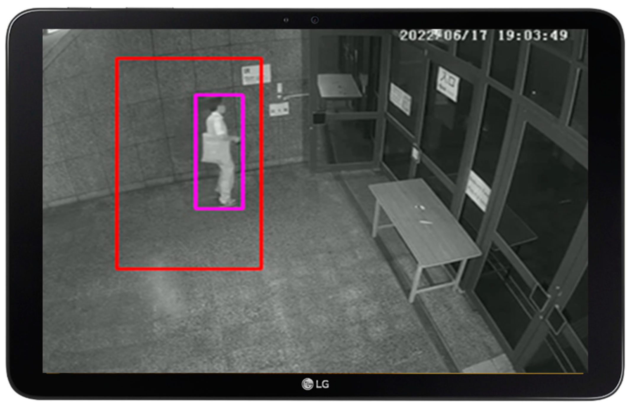
What sets Yolo apart is its groundbreaking concept of single-shot detection, signifying its ability to detect and classify objects in an image during a single pass through a neural network. This innovative approach culminates in the prediction of bounding boxes, exemplified by the pink square box in Figure 1, which encompasses the identified objects. Similar objectives can be identified using the structural similarity index measure (SSIM) [5] and vision transformer (ViT) [6], both of which are efficient object detection algorithms.

Hence, object detection using Yolo finds wide-ranging practical applications, including security surveillance, where it excels at identifying and tracking individuals or moving objects within security camera footage. This paper presents FenceTalk, a user-friendly moving object detection system. FenceTalk adopts a no-code approach, allowing non-AI expert users to effortlessly track the objects they define. In Section 5, we will carry out a performance comparison between FenceTalk and the previously proposed approaches.

Figure 1 illustrates the window-based FenceTalk graphical user interface (GUI), where a red polygon can be easily created by dragging an area of interest. This area is designated as a fenced region within a fixed location. Through deep learning models, image recognition is performed to detect the presence of moving objects (depicted by the pink square in Figure 1) within the fenced area.

Combining with IoTtalk, an IoT application development platform [7], FenceTalk sends real-time alert messages to pre-bound devices through IoTtalk when a moving object is detected within the fenced area. This allows users to swiftly take appropriate measures to ensure the security of the area. A reliable image recognition model is crucial for FenceTalk. However, even after capturing images with targets in the desired new area for labeling and using this annotated data for training the deep learning model, the model often fails to recognize certain moving objects. Identifying these images where recognition was unsuccessful and using them as training data for the model can further enhance its accuracy.

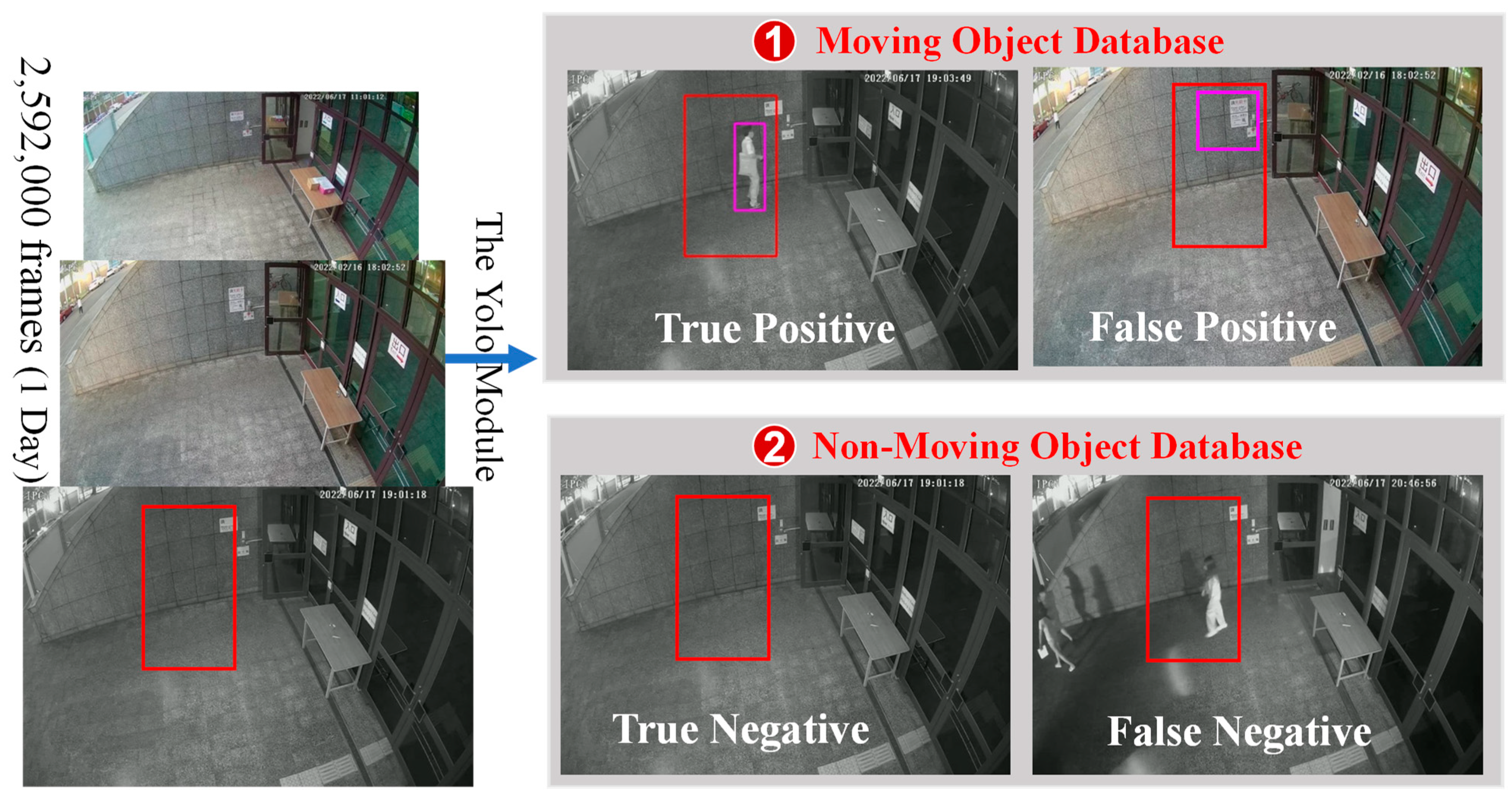
Extracting image frames containing moving objects from a vast amount of image data as training data for the model incurs significant labor and time costs. For instance, at the common camera recording rate of 30 frames per second (FPS), a camera can generate 2,592,000 image frames in a single day. Given that the moving objects to be recognized in a fixed area exhibit movement characteristics, FenceTalk designs an algorithm to define a background image, and compares the current image frame with the background image using SSIM to analyze differences in the images. Subsequently, based on the brightness of the current image, FenceTalk employs an optimal threshold to separate background noise from the moving objects of interest. This process determines whether the current image frame contains a suspicious image with moving objects. By filtering these selected suspicious images, FenceTalk enables users to choose the model’s training data with reduced human resource costs. To minimize hardware costs, we deployed FenceTalk on an embedded device, the Nvidia Jetson Nano, equipped with a graphics processing unit. The Jetson Nano GPU features 128 CUDA cores and 4 GB LPDDR4 memory, making it suitable for running CNN models that require extensive matrix operations.

This paper is organized as follows: Section 2 reviews the previous work; Section 3 describes the FenceTalk architecture; Section 4 describes how SSIM is used in FenceTalk; Section 5 evaluates the object detection performance of FenceTalk and the time and space complexities of Nvidia Jetson Nano.

2. Related Works

Deep learning models for moving object detection based on CNNs [8,9,10,11] can utilize camera images from specific areas as training data to learn the features of moving objects. This enables accurate identification of moving objects within the frame. In a previous work [4], the authors chose the Yolo model for recognizing humans and vehicles, applying it to a real-time recognition system in an advanced driver assistance system (ADAS). Compared to two-stage recognition models like Faster-RCNN, the one-stage Yolo model strikes a balance between accuracy and speed. Yolo and Yolo-tiny were employed for pedestrian detection, achieving a recall rate of more than 80%. Yolo-tiny, in particular, is well-suited to scenarios requiring real-time detection—aligning with the application context of FenceTalk in our study.

We evaluated different versions of YOLO [12,13]. Despite YOLOv6 [14] having 33% fewer parameters than YOLOv7-tiny and YOLOv4-tiny at the same scale, its inference speed improved by less than 10%. However, this reduction in parameters led to an accuracy drop of nearly 10% compared to YOLOv7-tiny. YOLOv7-tiny’s optimization primarily emphasizes training efficiency and inference speed. On our hardware, YOLOv7-tiny demonstrated object detection approximately 10% faster than that of YOLOv4-tiny. Nevertheless, YOLOv7-tiny only achieved an accuracy of 90.86% on our dataset, falling short of YOLOv4-tiny’s performance. As a result, we ultimately opted for YOLOv4-tiny as our choice.

Now we review the past methods for evaluating image similarity and the applications related to SSIM. Mean square error (MSE) is a common and straightforward approach to measure the similarity between two images. It calculates the mean squared error value of image pixels as an indicator of image similarity. A higher MSE value indicates greater disparity between the two images. The calculation method of MSE considers only the corresponding pixel values of the two images, making its results less reliable. In a study [15], using Einstein’s image as an example, JPEG image compression and blurring were applied, resulting in significant differences between the two images. However, their MSE results were similar to the original image. MSE can also exhibit substantial variations in values due to minor pixel rearrangements. The authors of the study slightly shifted and scaled the Einstein image, maintaining a similar appearance to the original. Nevertheless, the MSE values for these modified images were significantly high, reaching 871 and 873, respectively, compared to the original image.

Peak signal-to-noise ratio (PSNR) [16] is defined based on MSE and is also widely used for measuring image similarity [17]. PSNR resolves this issue by incorporating peak intensity considerations. In particular, the logarithmic transformation enables us to express scores more concisely. Consequently, the advantages of PSNR over MSE can be summarized as follows: (1) facilitating the comparison of results obtained from images encoded with varying bit depths and (2) providing a more concise representation. However, it is important to note that, by definition, PSNR remains essentially a normalized variant of MSE. PSNR finds widespread utility in tasks related to image and video compression, restoration, and enhancement, effectively quantifying the extent of information loss during compression or processing. A higher PSNR value indicates greater similarity between the two images. Nevertheless, when it comes to background detection, it does not exhibit the same effectiveness as mixture of Gaussians (MOG) [18] and absolute difference (AD) [19].

MOG [18] is purpose-built for modeling the background within images by employing a mixture of Gaussian distributions. MOG demonstrates adaptability to changing lighting conditions and exhibits robust performance across various scenarios, making it suitable for real-time applications. AD [19] represents another background subtraction technique. While specific implementation details may vary, the core concept is to calculate the absolute pixel-wise difference between corresponding pixels in two input images. The result is a new image, known as the absolute difference image. Specifically, MOG garners favor for its robustness in accommodating evolving environments, whereas the efficacy of AD hinges on pixel-wise absolute difference.

In [20], it is argued that natural images possess highly structured characteristics with closely related neighboring pixels. As a result, the structural similarity index measure (SSIM) was introduced. SSIM is designed based on the human visual system (HVS) and evaluates image similarity by considering brightness, contrast, and structural factors. Unlike traditional methods like MSE or PSNR, which use a sum of errors, SSIM does not drastically change its results due to minor changes in image brightness or noise, better aligning with the human perception of image quality. The calculation method of SSIM will be further introduced in Section 4.

In [21], the authors advocate using SSIM to measure the distance between tracked objects and candidate bounding boxes in object tracking. Unlike the traditional method of object tracking based on object color classification, this paper demonstrates that even in challenging conditions such as temporary occlusion or changes in image brightness, using SSIM still yields stable and reliable object tracking results.

In [22], the authors compare detection methods for moving objects using a single Gaussian model, an adaptive Gaussian mixture model 2 (MOG2), and SSIM-based approaches. The traditional single Gaussian model tends to capture a significant amount of image noise, while MOG2 struggles to detect targets with similar colors to the background. However, the SSIM-based detection method can accurately detect moving objects. The study only utilized the first frame of the video as the SSIM background image and did not consider subsequent changes in the background. In contrast, FenceTalk incorporates an algorithm to update the SSIM background image and validates its stability using a large dataset.

In [23], a method for detecting geometric defects in digital printing images is proposed based on SSIM. The study inspects defects such as stains, scratches, and ink in simulated and real images. Compared to the AD-based inspection method, the SSIM-based approach effectively detects subtle defects and reduces misjudgments caused by environmental lighting factors.

ViT [6] is the state-of-the-art model for image classification, which is a revolutionary deep learning architecture that has gained significant attention and popularity in the field of computer vision. ViT has powerful image recognition capabilities, and when used for image classification, it can achieve excellent results. Based on practical experience, ViT’s performance significantly surpasses that of earlier algorithms MSE, PSNR, MOG2, and AD. While running ViT does consume a significant amount of computational resources, its performance can serve as an upper-bound reference point for accuracy comparison.

In a home security automatic recording system described in [24], SSIM is used to compare the current and the next image frames to decide whether to trigger the recording process. This system achieves a high-accuracy and stable event detection, saving storage space and simplifying subsequent image analysis time. While the study used an average similarity index and standard deviation of 100 consecutive pairs of frames as the threshold for motion detection, FenceTalk differentiates images based on brightness to find the optimal threshold. It then separates background noise and moving objects using this threshold, automatically selecting images that Yolo failed to recognize. This reduces the time cost of manual labeling. The study reported a motion detection accuracy ranging from 0.985 to 0.995 in most experiments, while FenceTalk achieves a slightly better performance of 0.9994. In [25], SSIM-NET is introduced for defect detection in printed circuit boards (PCBs). SSIM-NET employs a two-stage approach where SSIM identifies regions of interest in the image, followed by classification using MobileNet-V3. Compared to Faster-RCNN, SSIM-NET offers more than 12 times faster recognition speed, 0.62% higher accuracy, and faster training time. However, unlike FenceTalk, PCB defect detection does not need to consider the impact of abrupt lighting changes on SSIM, and the paper does not mention how SSIM background images are updated.

3. FenceTalk Architecture

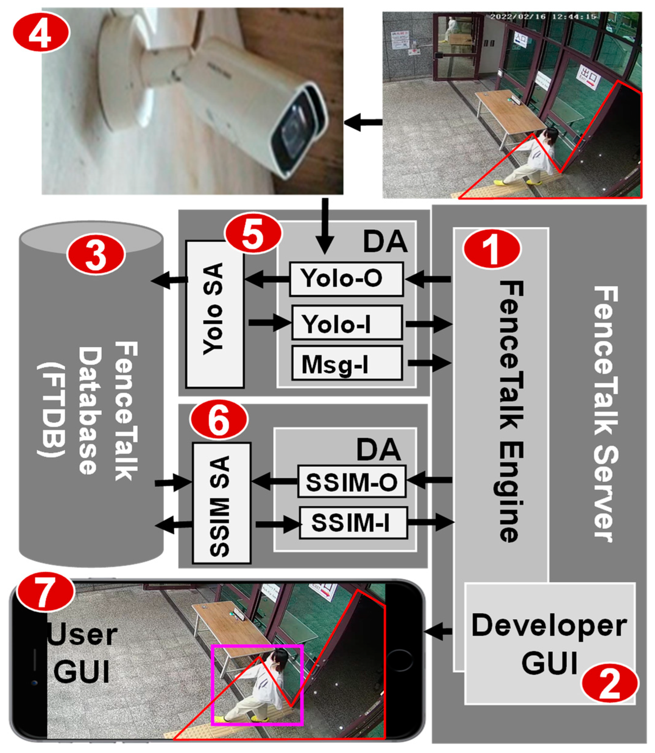
FenceTalk utilizes a network camera to transmit real-time images for image recognition. Figure 2 illustrates the FenceTalk architecture, comprising six key components. At its core is the FenceTalk server, which includes the FenceTalk engine (Figure 2 (1)), derived from IoTtalk [6], and a developer GUI (Figure 2 (2)). Following the IoTtalk philosophy, the FenceTalk server operates as an IoT server and employs an image database known as FenceTalk DataBase (FTDB) to store images extracted from the video streams (Figure 2 (3)). Additionally, the remaining four components within FenceTalk serve as IoT devices, encompassing the camera software module (Figure 2 (4)), the Yolo module (Figure 2 (5)), the SSIM module (Figure 2 (6)), and the user GUI module (Figure 2 (7)).

Each of these software modules consists of two parts: device application (DA) and sensor and actuator application (SA). The DA is responsible for communication with the FenceTalk server using HTTP communication ((5)$\leftrightarrow$(1), (6)$\leftrightarrow$(1), (7)$\leftrightarrow$(1) in Figure 2), which can be achieved through wired means (e.g., Ethernet) or wireless options (e.g., 5G or Wi-Fi) for communication. The SA part implements functionalities related to IoT devices, such as Yolo SA for object detection based on the Yolo model and SSIM SA for detecting moving objects based on SSIM.

The network camera (Figure 2 (4)) uses the real-time streaming protocol (RTSP) to stream the image frames. If the user draws a red polygon to define a fenced area within the desired field, FenceTalk will exclusively perform object detection within this specified area. The Yolo SA (Figure 2 (5)) continuously receives the latest streaming image frames and conducts object detection within the designated region using the Yolov4-tiny model. The results of the detection process, including object names, positions, and image paths, are stored in FTDB (Figure 2 (3)).

The ongoing Yolo recognition result is transmitted to the FenceTalk Engine (Figure 2 (1)) through the DA interface Yolo-I. The engine receives this data and has the capability to preprocess it using custom functions before transmitting it to connected IoT devices. Specifically, the engine forwards the Yolo recognition results to SSIM (Figure 2 (6)) through the DA interface SSIM-O for further evaluation. The outcomes of this evaluation, which include information about the presence of moving objects and corresponding image paths, are then stored in FTDB. Simultaneously, the SSIM assessment result is sent to the FenceTalk server via the DA interface SSIM-I, which is sent back to the Yolo module for further processing (See Section 4). The results of object recognition are subsequently displayed on user-defined devices (Figure 2 (7)).

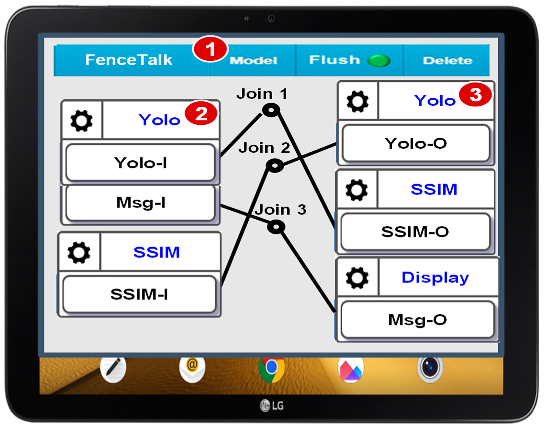
In FenceTalk, IoT devices can be effortlessly connected and configured using the developer GUI (Figure 2 (2)) accessible through a web browser. Figure 3 depicts this GUI, wherein the involved IoT devices can be chosen from the model pulldown list (Figure 3 (1)). When we opt for the Yolo IoT device (i.e., the Yolo module), two icons are displayed within the GUI window. The icon on the left side of the window indicates the DA interfaces Yolo-I and Msg-I (Figure 3 (2)). The icon on the right side represents the DA interface Yolo-O (Figure 3 (3)). Similarly, we can choose the SSIM and the display devices. To establish connections between the IoT devices, all that is required is dragging the “join links.” For instance, Join 1 connects Yolo-I to SSIM-O. This link creates an automatic communication pathway between the Yolo module and the SSIM module. Consequently, the configuration shown in Figure 3 yields the FenceTalk architecture displayed in Figure 2.

4. The SSIM Module

When the Yolo module processes an image and detects the moving objects, it places the image in the moving object database (Figure 4 (1)). If no moving objects are detected, the image is placed in the non-moving object database (Figure 4 (2)). Both databases are parts of FTDB (Figure 2 (3)). The detection accuracy of the Yolo module can be improved through re-training using false positive images from the moving object database and false negative images from the non-moving object database. The identification of false positive/negative images is typically performed manually. Unfortunately, our experience indicates that the size of the non-moving object database is usually substantial, making the identification of false positive images a highly tedious task. To resolve this issue, we developed the SSIM module.

The structural similarity index (SSIM) is a metric used to measure the similarity between two images. It assesses the images based on their brightness, contrast, and structural similarity. It is commonly employed to determine the degree of similarity or distortion between two images. Given a background image $x$ and a test photo $y$, both of size $m\times n$, SSIM is defined as:

$$\mathrm{S}\mathrm{S}\mathrm{I}\mathrm{M}\left(x,y\right)={\left[\mathsf{\Psi }\left(x,y\right)\right]}^{\alpha }{\left[c\left(x,y\right)\right]}^{\beta }{\left[s\left(x,y\right)\right]}^{\gamma }$$

(1)

where

$$\mathsf{\Psi }\left(x,y\right)=\frac{2{\mu }_x{\mu }_y+C_1}{{\mu }_x^2+{\mu }_y^2+C_1}$$

(2)

$$c\left(x,y\right)=\frac{2{\sigma }_x{\sigma }_y+C_2}{{\sigma }_x^2+{\sigma }_y^2+C_2}$$

(3)

$$s\left(x,y\right)=\frac{{\sigma }_{xy}+C_3}{{\sigma }_x{\sigma }_x+C_3}$$

(4)

In $\mathsf{\Psi }$(x, y), grayscale values of the images are used to compare the similarity in average luminance between the two images. In the function c(x, y), contrast similarity between the images is assessed by calculating the standard deviation of image pixels. The function s(x, y) measures the similarity in structural content between the two photographs. In Equation (2), ${\mu }_x$ and ${\mu }_y$ represent the average values of the pixel intensities of the two images, while ${\sigma }_x$ and ${\sigma }_y$ in Equations (3) and (4) denote the covariance of the two images. Constants $C_1$, $C_2$, and $C_3$ are used to stabilize the function, where $C_1={K_{1}L}^2$, $C_2={K_{2}L}^2,$ and $C_3=\frac{C_2}{2}$. The values of $K_1$ and $K_2$ are set as 0.01 and 0.03, respectively, and $L$ is the number of possible intensity levels in the image. For an 8-bit grayscale image, L would be 255. In [20], the values of $\alpha$, $\beta$, and $\gamma$ are set to 1, leading to a simplified SSIM formula of Equation (1):

$$\mathrm{S}\mathrm{S}\mathrm{I}\mathrm{M}\left(x,y\right)=\frac{\left(2{\mu }_x{\mu }_y+C_1\right)\left(2{\sigma }_{xy}+C_2\right)}{\left({{\mu }_x}^2+{{\mu }_y}^2+C_1\right)\left({{\sigma }_x}^2+{{\sigma }_y}^2+C_2\right)}$$

(5)

The structural similarity index (SSIM) yields larger values for more similar images and possesses three key properties. The symmetry property is

$$\mathrm{S}\mathrm{S}\mathrm{I}\mathrm{M}\left(x,y\right)=\mathrm{S}\mathrm{S}\mathrm{I}\mathrm{M}\left(y,x\right)$$

The bound property is

SSIM(x, y) ≤ 1

The uniqueness property states that when two images are identical, i.e., ${\mu }_x={\mu }_y$ and ${\sigma }_x={\sigma }_y$, we have

SSIM(x, y) = 1

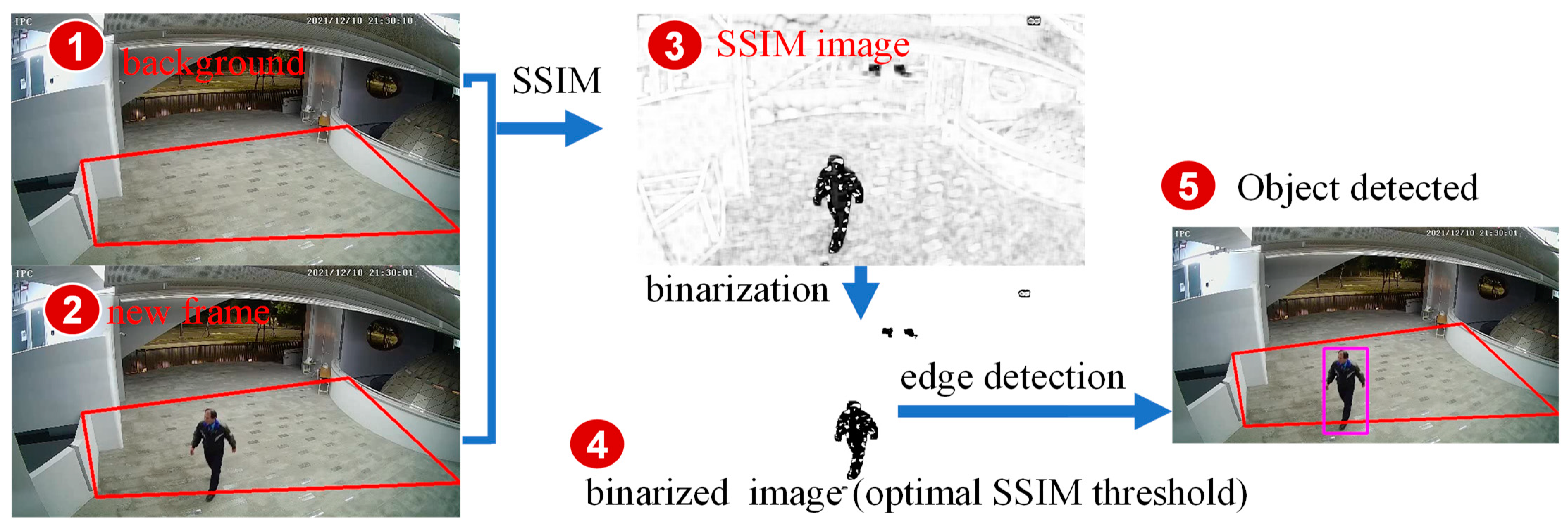
FenceTalk utilizes a predefined background image (Figure 5 (1)) and an image frame (Figure 5 (2)) to determine the presence of moving objects. Since SSIM requires two single-channel image frames as input, we convert the input images from RGB with three channels to single-channel grayscale images. Then, we use an $N\times N$ sliding window with a moving stride of 1. For each window, the SSIM is calculated. The output range of SSIM is [0, 1], while the pixel values of an 8-bit image are in the range of [0, 255]. To represent the SSIM values obtained from each sliding window in the full range of grayscale values, we linearly scale the SSIM values to the range of [0, 255]. This produces a complete single-channel grayscale (binarized) SSIM image (Figure 5 (3)).

In the SSIM image, different degrees of differences are represented by varying shades of color. When the difference between the two images within a sliding window is larger, the SSIM value is lower, and the corresponding area on the SSIM output image is represented by darker shades. Conversely, when the difference between the two images within a sliding window is smaller, the SSIM value is higher, and the corresponding area on the SSIM output image is represented by lighter shades.

To determine the presence of moving objects in the SSIM image, a threshold value needs to be set to separate the background noise from the moving objects. Using Figure 5 (3) as an example, a threshold value of 125 is applied to this SSIM image to obtain the image in Figure 5 (4). This process involves image binarization and edge detection, filtering out small noise components, and determining whether the area within the fence boundary contains moving objects. The corresponding detection positions are then highlighted on the RGB image (Figure 5 (5)). The selection of an appropriate threshold to effectively distinguish background noise from moving objects will be further discussed and experimentally demonstrated in the next section.

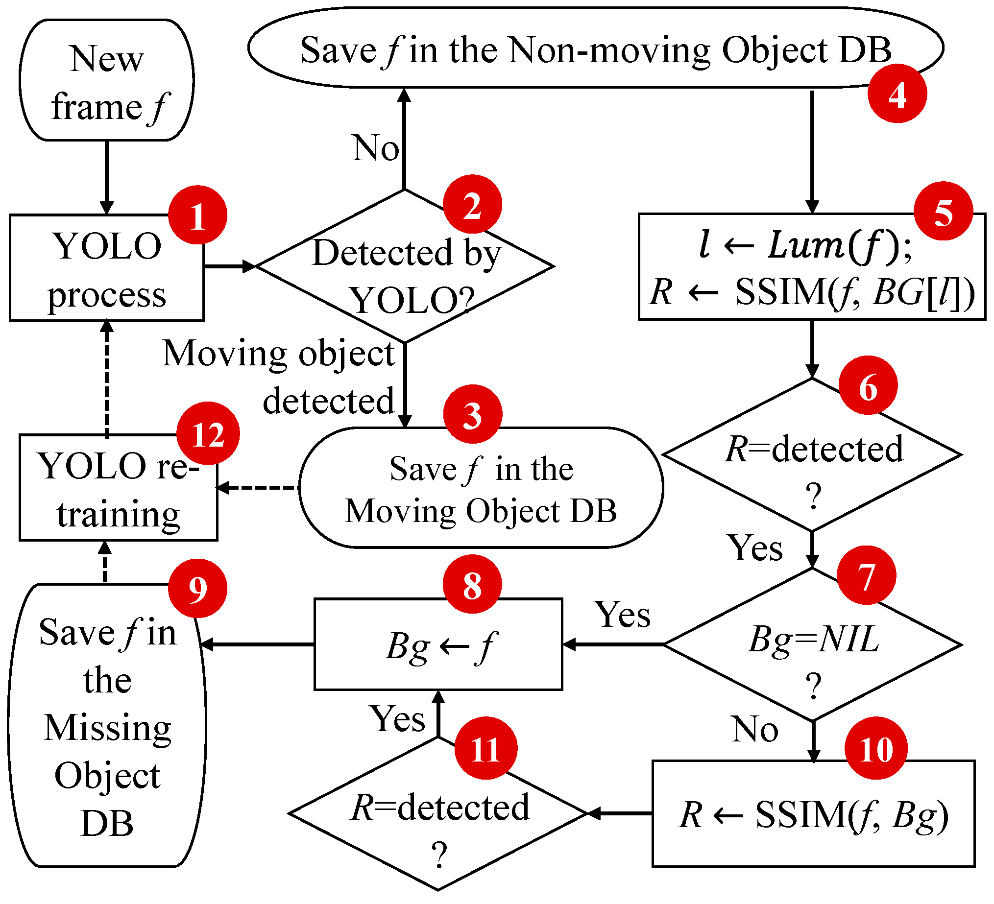
The flowchart of the Yolo and the SSIM modules is illustrated in Figure 6. FenceTalk determines the presence of moving objects by comparing the current frame with a background image. Before processing the image frame detection, FenceTalk selects frames with varying brightness from the video as candidate background images, denoted as BG[l] ($0\le l\le L=255$). If the moving objects to be recognized are within the 80 classes of the MS COCO dataset [26], these candidate backgrounds are initially processed by a pre-trained Yolo model trained on the MS COCO dataset to identify images that do not contain the moving object (e.g., people). However, due to limitations in the pre-trained Yolo model’s recognition capabilities or when the moving object is not in the MS COCO dataset, users need to examine and remove background images that FenceTalk incorrectly identified as not containing any moving objects. In FenceTalk, moving objects are defined as objects that change their position relative to the background image over time, i.e., they are not fixed in the background.

FenceTalk reads a predefined background image BG[l] at the brightness level l, and from the video, it reads the next frame f to be processed. Frame f first undergoes the Yolo module for object recognition (Figure 6 (1)), where the Yolo model can be a pre-trained model on the MS COCO dataset or a user-trained model. If the Yolo module detects any objects (Figure 6 (2)), the images containing the moving objects are stored in the moving object database (Figure 6 (3)), and those without the moving object are stored in the non-moving object database (Figure 6 (4)). The process then moves on to the next frame. If the Yolo module does not detect any objects, FenceTalk enters the SSIM module to detect the false negatives images in the non-moving object database. The non-moving object database serves as a buffer due to the differing processing speeds of the Yolo module, which utilizes GPU, and the SSIM module, which operate on CPU. Consequently, the non-moving object database guarantees that all images from the Yolo module can be processed by the SSIM module without any loss of images.

FenceTalk calculates the brightness of frame f as l and selects the background image BG[l] with the same or closest brightness to f. The SSIM module then detects missing moving objects by comparing f and BG[l] (Figure 6 (5)). If the detection result (Figure 6 (6)) does not contain moving objects, the process continues to the next frame.

To reduce false positives caused by changes in background lighting or the addition of new objects to the background, if FenceTalk determines that f contains moving objects (Figure 6 (6)), it performs a second check using a secondary background image, Bg. Initially, FenceTalk checks if background image Bg exists (Figure 6 (7)). If Bg does not exist (Initially, Bg = NIL), f is set as Bg (Figure 6 (8)) and stored (Figure 6 (9)) for subsequent model training. If Bg exists, SSIM is again applied to detect moving objects by comparing f and Bg (Figure 6 (10)). If the detection result (Figure 6 (11)) does not contain moving objects, the process continues to the next frame. If moving objects are detected, Bg is replace by f (Figure 6 (8)), and f is stored in the missing object database (Figure 6 (9)). The purpose of Bg is to prevent the repetitive detection and storage of the same moving object across a sequence of consecutive images. The utilization of SSIM(f, Bg) (Figure 6 (10)) ensures that each moving object is saved in the missing object database only once. After processing all desired image frames, users can retrieve all identified moving objects (Figure 6 (3)) and missing objects (Figure 6 (9)) from the database. These false negative images can be automatically annotated and used to retrain the Yolo model (Figure 6 (12)) to improve its accuracy. The retrained Yolo model can then be used to repeat the recognition process (Figure 6 (1)) for improved recognition accuracy.

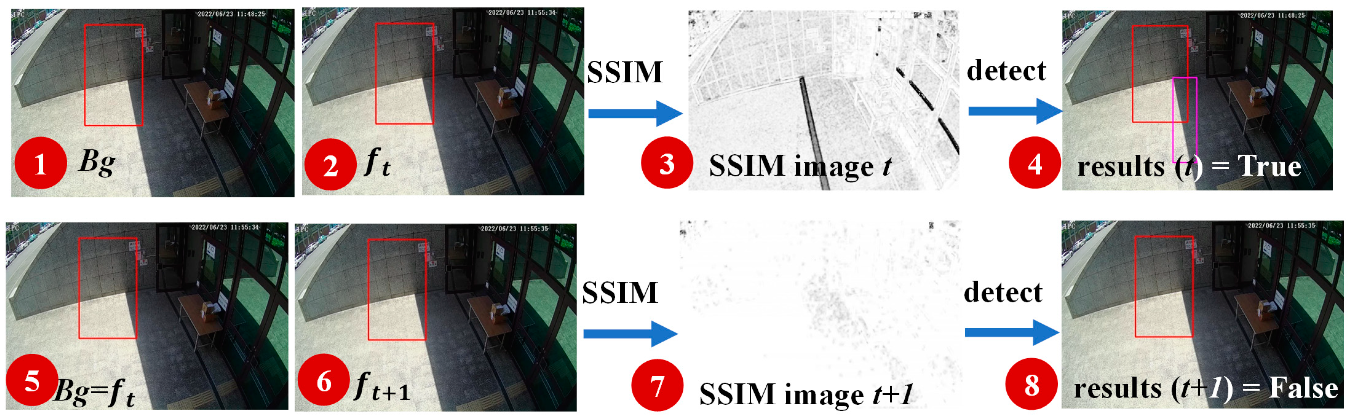
Figure 7 illustrates the process of automatic background update. The SSIM image (Figure 7 (3)) is generated by comparing the background image (Figure 7 (1)) with the current image frame $f_t$ at time $t$ (Figure 7 (2)). Noticeable changes in shadows can lead to misjudgment of moving objects by FenceTalk (Figure 7 (4)). Upon detecting moving objects, FenceTalk updates the background image (Figure 7 (5)). The SSIM image (Figure 7 (7)) is generated by comparing the updated background image with the subsequent image frame $f_{t+1}$ at time $t+1$ (Figure 7 (6)). The result is a correct judgment that the image frame $f_{t+1}$does not contain any moving objects (Figure 7 (8)).

5. FenceTalk Experiments

This section describes the datasets we collected and explains how we utilized these data to experimentally demonstrate the universality of the optimal threshold for SSIM. We will also discuss the accuracy of SSIM and Yolo in different subsets of the dataset. Finally, we will showcase the processing speed and resource usage of FenceTalk on the embedded device Jetson Nano.

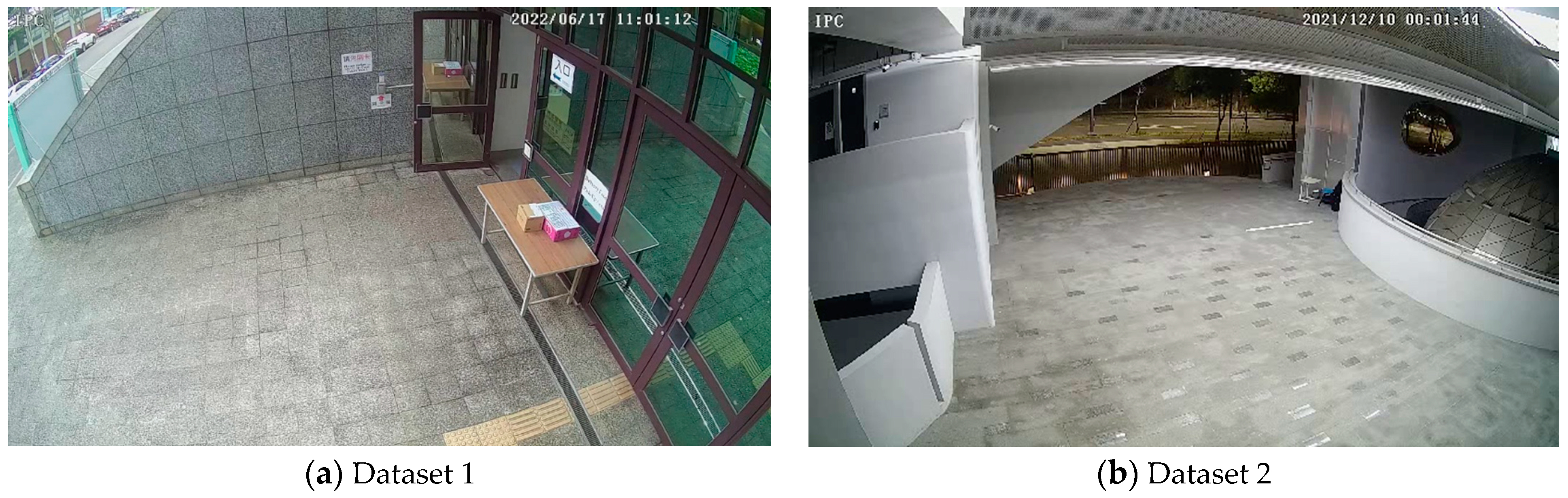
We collected continuous camera footage from two outdoor locations, National Yang Ming Chiao Tung University and China Medical University, for a duration of six days each, using a recording frame rate of 30 FPS. Compared to indoor stable lighting conditions, the use of outdoor camera footage from these two locations provided a more robust evaluation of FenceTalk’s performance in complex lighting environments. Dataset 1 was obtained from the entrance of the Electronic Information Building at No. 1001 University Road, National Yang Ming Chiao Tung University, Hsinchu City (as shown in Figure 8a). The data collection period was from 17 June 2022 to 23 June 2022, covering the entire day’s camera footage. Dataset 2 was gathered from the Innovation and Research Building at No. 100, Section 1, Jingmao Road, Beitun District, China Medical University, Taichung City (as shown in Figure 8b). The data collection period spanned from 10 December 2021 to 15 December 2022, capturing the full day’s camera footage. In Dataset 1, images were collected at a rate of 10 FPS, resulting in a total of 4,832,579 images. Among these, there were 226,518 images containing moving objects (people). Dataset 2 comprised images collected at a rate of 15 FPS, with a total of 6,910,580 images. Within this dataset, 144,761 images were of moving objects. All images had a resolution of 1920 × 1080 pixels. These datasets were chosen to encompass a diverse range of lighting conditions and scenarios, enabling us to validate FenceTalk’s performance robustness and reliability in real-world outdoor environments. It is noteworthy that due to this high collection frequency, the contents of any two consecutive images exhibited striking similarity. When it came to utilizing these images in training our model, a straightforward approach proved to be counterproductive, as it substantially consumed computational resources without yielding significant benefits to the model’s performance. Therefore, we resampled the images at a rate of 5 FPS, which captured one image every 0.2 s. This adjustment allowed us to maintain a sufficiently fast capture rate to effectively track moving objects (people), and train a highly effective model while conserving computational power.

Table 1. The images for training, validation, and testing.

Dataset 1	No. of Images	No. of Images with People
Training	862,258	23,098
Validation	808,153	35,358
Testing	786,443	40,700
Dataset 2
Training	496,936	22,805
Validation	479,452	20,025
Testing	402,265	19,003

shows the total number of images utilized in Datasets 1 and 2 after the resampling process.

We utilized standard output measures for AI predictions, distinguishing them for the Yolo module, the SSIM module, and FenceTalk (Yolo + SSIM). All images processed by the Yolo module were classified into the following categories: TP (true positives), TN (true negatives), FN (false negatives), and FP (false positives). Therefore, we have

$$\mathrm{Y}\mathrm{o}\mathrm{l}\mathrm{o}: \mathrm{P}\mathrm{r}\mathrm{e}\mathrm{c}\mathrm{i}\mathrm{s}\mathrm{i}\mathrm{o}\mathrm{n}=\frac{TP}{TP+FP} \mathrm{a}\mathrm{n}\mathrm{d} \mathrm{R}\mathrm{e}\mathrm{c}\mathrm{a}\mathrm{l}\mathrm{l}=\frac{TP}{TP+FN}$$

(6)

In the SSIM module, the images in the non-moving object database were classified into ${TP}^{*}$ true positives, ${TN}^{*}$ true negatives, ${FN}^{*}$ false negatives, and ${FP}^{*}$ false positives. Therefore, we have

$$\mathrm{S}\mathrm{S}\mathrm{I}\mathrm{M}: \mathrm{P}\mathrm{r}\mathrm{e}\mathrm{c}\mathrm{i}\mathrm{s}\mathrm{i}\mathrm{o}\mathrm{n}=\frac{{TP}^{*}}{{TP}^{*}+{FP}^{*}} \mathrm{a}\mathrm{n}\mathrm{d}\mathrm{R}\mathrm{e}\mathrm{c}\mathrm{a}\mathrm{l}\mathrm{l}=\frac{{TP}^{*}}{{TP}^{*}+{FP}^{*}}$$

(7)

and finally, the output measures for FenceTalk (Yolo + SSIM) are

$$\mathrm{F}\mathrm{e}\mathrm{n}\mathrm{c}\mathrm{e}\mathrm{T}\mathrm{a}\mathrm{l}\mathrm{k}: \mathrm{P}\mathrm{r}\mathrm{e}\mathrm{c}\mathrm{i}\mathrm{s}\mathrm{i}\mathrm{o}\mathrm{n}=\frac{TP+{TP}^{*}}{{TP+FP+TP}^{*}+{FP}^{*}}$$

(8)

and

$$\mathrm{F}\mathrm{e}\mathrm{n}\mathrm{c}\mathrm{e}\mathrm{T}\mathrm{a}\mathrm{l}\mathrm{k}:\mathrm{R}\mathrm{e}\mathrm{c}\mathrm{a}\mathrm{l}\mathrm{l}=\frac{TP+{TP}^{*}}{TP+FN}$$

(9)

Specifically, the total count of all moving objects within a dataset is derived by TP + FN. The count of correctly predicted cases by Yolo is represented by TP. TP* represents the count of accurately predicted cases by SSIM among the FN cases. Consequently, the total count of correctly predicted cases by FenceTalk (Yolo + SSIM) is TP + TP*. Therefore, the recall is calculated as TP + TP*/TP + FN. The F1 score is expressed as

$$\mathrm{F}1\mathrm{s}\mathrm{c}\mathrm{o}\mathrm{r}\mathrm{e}=2\left(\frac{\mathrm{P}\mathrm{r}\mathrm{e}\mathrm{c}\mathrm{i}\mathrm{s}\mathrm{i}\mathrm{o}\mathrm{n}\times \mathrm{R}\mathrm{e}\mathrm{c}\mathrm{a}\mathrm{l}\mathrm{l}}{\mathrm{P}\mathrm{r}\mathrm{e}\mathrm{c}\mathrm{i}\mathrm{s}\mathrm{i}\mathrm{o}\mathrm{n}+\mathrm{R}\mathrm{e}\mathrm{c}\mathrm{a}\mathrm{l}\mathrm{l}}\right)$$

(10)

In Equation (10), the F1 score takes into account both precision and recall.

In FenceTalk, to find and verify the universality of the optimal SSIM threshold in each dataset, we divided each dataset into three subsets: the training dataset, the validation dataset, and the testing dataset. In the FenceTalk experiments, we calculated the precision and recall for both Yolo and SSIM (Equations (6) and (7)).

To find the optimal SSIM threshold, we calculated the average grayscale value of each image and used it as an image brightness category. We used an interval of 25 for the SSIM threshold and recorded the $TP$, $TN$, $FN$, and $FP$ counts for different thresholds under various brightness levels. This helped us calculate the precision and recall of SSIM at different thresholds (elaborated in Figure 9 and Figure 10). Since we aimed to collect images that Yolo failed to recognize using SSIM for model training, we selected the threshold with the highest recall value as the optimal SSIM threshold for each brightness level in the experiment. If there were multiple highest recall values for a particular brightness level, we chose the threshold with the best precision among them. If duplicates remained, we selected the median as the optimal threshold.

We employed the modified Yolo model trained on the training dataset to test the validation dataset and find the optimal SSIM threshold for different brightness levels in this dataset. Using the optimal SSIM threshold from the validation dataset, we identified images containing moving objects and images detected by the Yolo model. After manual labeling, these images were combined with all images containing humans from the training dataset, serving as training data for the Yolo model, which was then applied to the testing dataset for inferencing.

Table 2. The output measures for Dataset 1 (red font signifies the best performance).

Dataset 1	Yolo			SSIM			Yolo + SSIM
	Precision	Recall	F1 Score	Precision	Recall	F1 Score	Precision	Recall	F1 Score
Training dataset (optimal SSIM thresholds from training dataset)	97.71%	77.16%	86.21%	97.99%	94.09%	96.00%	97.71%	98.68%	98.19%
Validation dataset (optimal SSIM thresholds from training dataset)	97.72%	92.42%	93.63%	96.74%	90.71%	93.63%	97.66%	99.30%	98.47%
Validation dataset (optimal SSIM thresholds from validation dataset)				97.59%	95.19%	96.37%	97.72%	99.64%	98.67%
Test dataset (optimal SSIM thresholds from training dataset)	97.67%	93.53%	95.59%	96.15%	92.93%	94.51%	97.64%	99.54%	98.58%
Test dataset (optimal SSIM thresholds from validation dataset)				96.29%	93.81%	95.03%	97.65%	99.75%	98.69%

presents the precision and recall of Yolo and SSIM using the optimal thresholds in Dataset 1. In the training phase, the recall for Yolo was relatively low at 77.16%. However, through the FenceTalk mechanism, the FenceTalk precision (Yolo + SSIM) was 97.71% and the recall (Yolo + SSIM) was 98.68%. The validation phase showed that FenceTalk’s precision exceeded 97% and FenceTalk’s recall (Yolo + SSIM) was above 99%. We re-trained the Yolo model after the validation phase. Therefore, the validation phase was a second training phase. Then, in the testing phase, FenceTalk’s precision was 97.65% and its recall was 99.75%.

Yolo’s core technology enables efficient and accurate real-time object detection, making it a fundamental tool in various computer vision applications. Yolo revolutionized object detection by introducing the concept of single-shot detection, meaning it can detect and classify objects in an image in a single forward pass of a neural network. Yolo places a strong emphasis on maintaining good precision, which in turn results in a lower recall. Yolo provides a confidence threshold to adjust the level of recall. A lower confidence threshold can achieve higher recall but may lead to lower precision. In Table 2 and

Table 3. The output measures for Dataset 2 (red font signifies the best performance).

Dataset 2	Yolo			SSIM			Yolo + SSIM
	Precision	Recall	F1 Score	Precision	Recall	F1 Score	Precision	Recall	F1 Score
Training dataset (optimal SSIM thresholds from training dataset)	98.81%	72.63%	83.72%	95.87%	94.12%	94.99%	98.81%	98.39%	98.2%
Validation dataset (optimal SSIM thresholds from training dataset)	97.89%	92.83%	95.65%	87.97%	89.62%	88.79%	97.89%	99.26%	98.57%
Validation dataset (Optimal SSIM thresholds from validation dataset)				88.66%	92.00%	90.29%	97.89%	99.43%	98.67%
Test dataset (optimal SSIM thresholds from training dataset)	98.55%	94.41%	96.59%	92.54%	91.06%	91.80%	98.54%	99.50%	99.02%
Test dataset (optimal SSIM thresholds from validation dataset)				93.03%	90.40%	91.70%	98.57%	99.67%	99.11%

, we show fine-tuning of the confidence threshold of Yolo to achieve a similar precision level as that of FenceTalk. Subsequently, we compared the differences in recall between Yolo and FenceTalk (Yolo + SSIM).

Table 3 presents the precision and recall of Yolo and SSIM using the optimal thresholds for Dataset 2. In the testing phase, FenceTalk’s precision was 98.57% and its recall was 99.67%. Both cases (Table 2 and Table 3) indicated that integrating SSIM into FenceTalk led to a further improvement in the overall F1 score compared to using only the Yolo model for recognition.

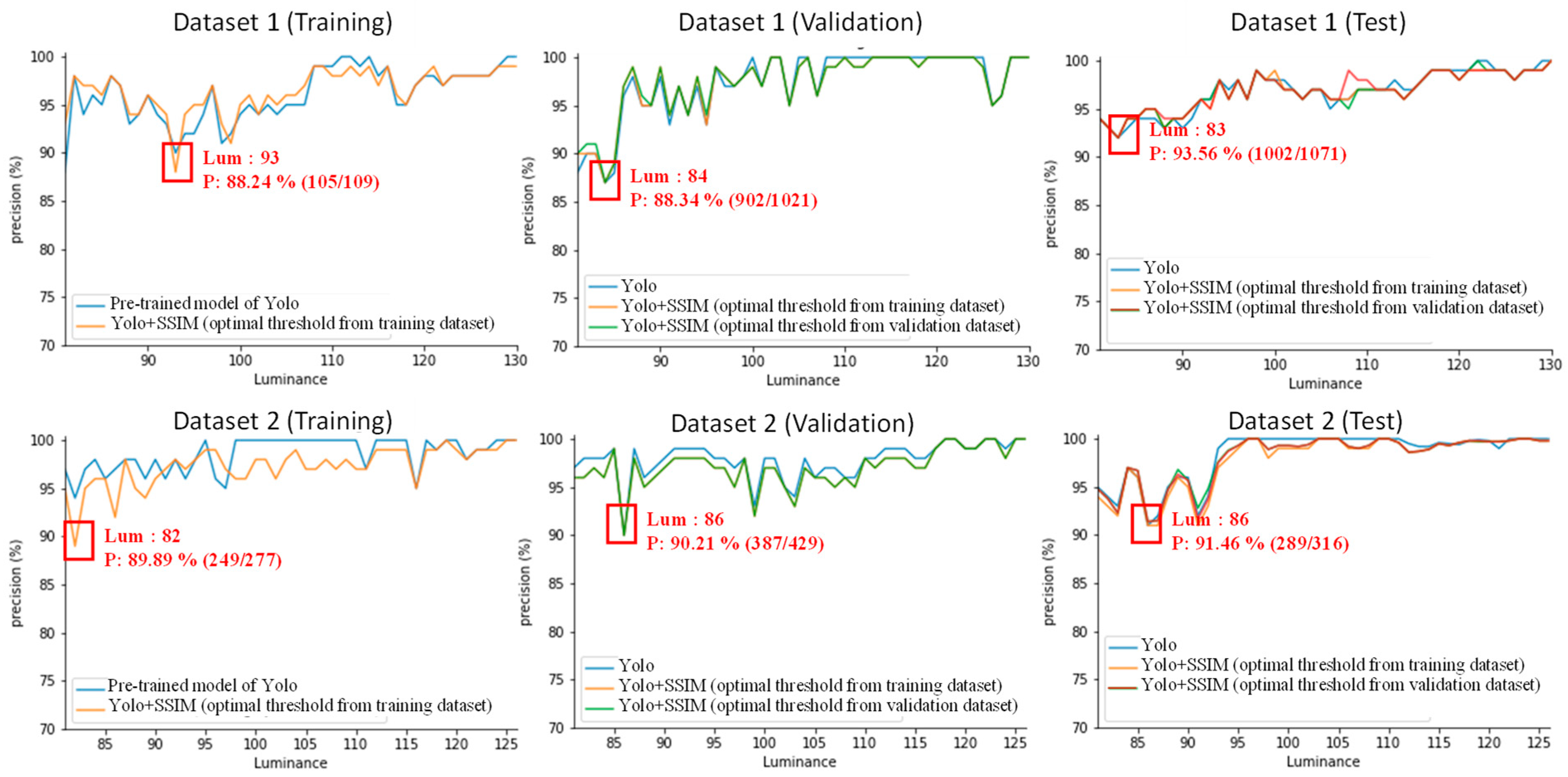
Figure 9 presents the precision accuracy of Yolo and SSIM under different sub-datasets and brightness levels. For Dataset 1, in the training phase, the lowest precision was 88.24% at brightness level 93. In the validation phase, the lowest precision was 87.34% at brightness level 84. In the testing phase, the lowest precision was 93.56% at brightness level 83. For Dataset 2, in the training phase, the lowest precision was 89.89% at brightness level 82. In the validation phase, the lowest precision was 90.21% at brightness level 86. In the testing phase, the lowest precision was 91.46% at brightness level 86.

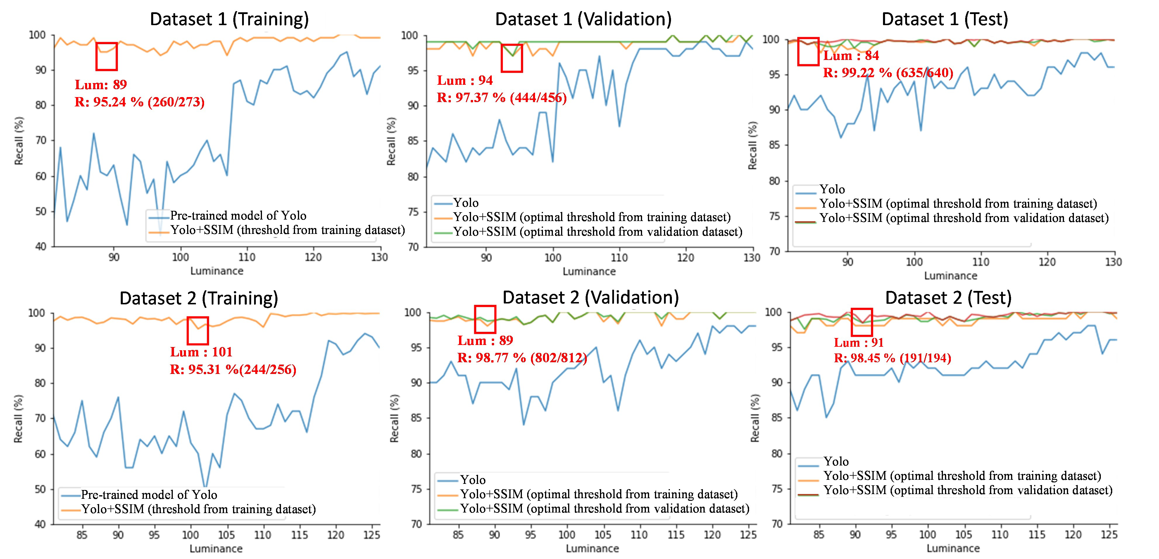
Figure 10 depicts the recall accuracy of Yolo and SSIM under different sub-datasets and brightness levels. For Dataset 1, in the training dataset, the lowest recall was 95.24% at brightness level 89. In the validation phase, the lowest recall was 97.37% at brightness level 94. In the testing dataset, the lowest recall was 99.22% at brightness level 84. For Dataset 2, in the training phase, the lowest recall was 95.31% at brightness level 101. In the validation phase, the lowest recall was 98.77% at brightness level 89. In the testing phase, the lowest recall was 98.45% at brightness level 98. Figure 9 and Figure 10 display the lowest precision and recall values across various sub-datasets and brightness levels. These lowest precision and recall metrics represent the baseline performance of FenceTalk. In the majority of cases, FenceTalk’s performance exceeded these lower bound values.

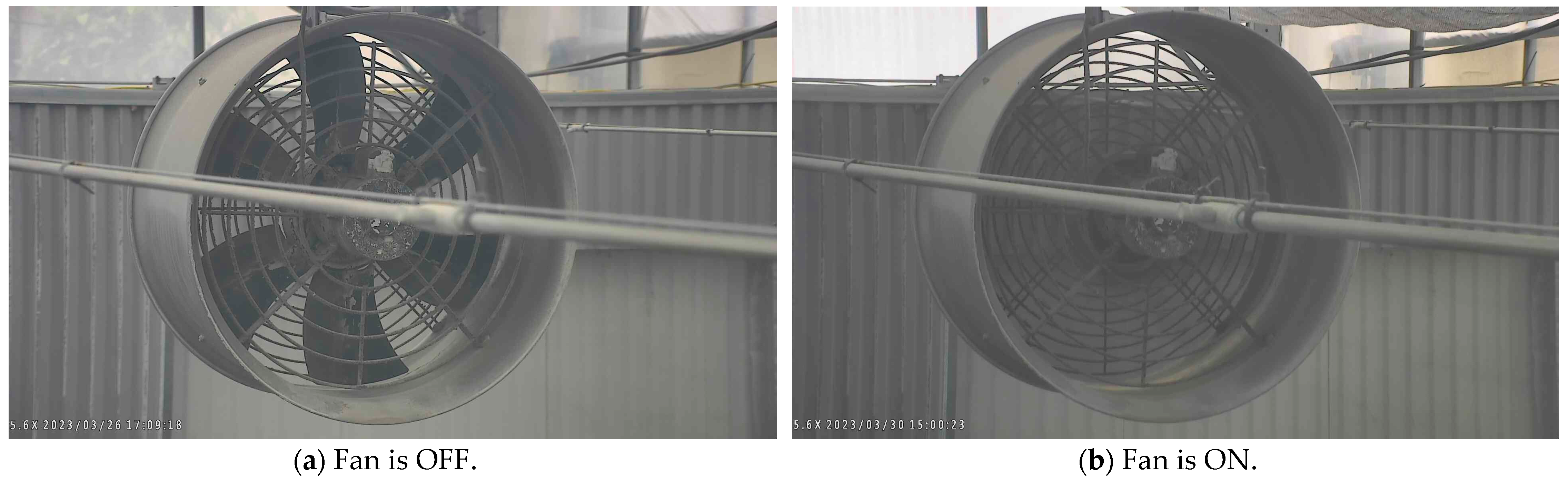
We also conducted a comparison of how ViT and SSIM performed in detection of moving objects. We applied ViT and SSIM in greenhouse equipment operation status detection. For instance, when a user turned on the exhaust fan (Figure 11), we checked whether the fan started correctly to determine the equipment’s normal operation.

Table 4. Performance of ViT.

ViT	Accuracy	Precision	Recall	F1-Score
Training (94,848 images)	0.999962	0.999860	1.0	0.999930
Validation (11,856 images)	0.999938	0.999716	1.0	0.999858
Testing (11,858 images)	0.999936	0.999642	1.0	0.999820

displays the performance of ViT in recognizing equipment operation status. ViT achieved a recall of 1 and an F1 score of 0.999.

Table 5. Performance of SSIM.

SSIM	Accuracy	Precision	Recall	F1-Score
Testing (23,712 images)	0.993158	0.989927	0.989314	0.989620

presents the results of SSIM, which were slightly lower than those of ViT. Specifically, SSIM achieved a recall of 0.98 and an F1 score of 0.989. These results indicate that SSIM can provide satisfactory performance when applied to moving object detection. However, when compared to ViT, SSIM requires significantly fewer computational resources.

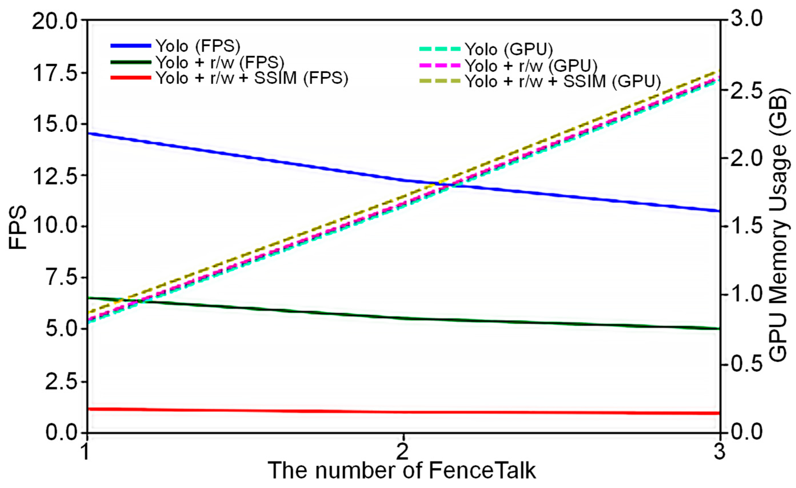
Figure 12 illustrates the processing speed and GPU utilization of the embedded device Jetson Nano when executing FenceTalk. Each instance of FenceTalk was capable of performing image recognition for an RTSP streaming camera. Yolo (FPS) and Yolo (GPU) represent the execution speed and memory usage of Jetson Nano during object recognition. Yolo + r/w (FPS) and Yolo + r/w (GPU represent the execution speed and memory usage when Jetson Nano performs object recognition and reads/writes images. Yolo + r/w + SSIM (FPS) and Yolo + r/w + SSIM (GPU) represent the execution speed and memory usage when Jetson Nano performs object recognition, reads/writes images, and employs SSIM for motion detection.

Our study indicates that Jetson Nano can simultaneously run up to three instances of FenceTalk (i.e., the sources of video streaming came from three cameras). When the number of FenceTalk instances was 1, Jetson Nano achieved a processing speed of 14.5 FPS during object recognition, utilizing 0.79 GB of memory. However, with 3 FenceTalk instances, the processing speed dropped to 10.7 FPS during object recognition, and the memory usage increased to 2.56 GB. As the number of FenceTalk instances increased, Jetson Nano’s processing speed decreased linearly rather than exponentially, while GPU utilization exhibited a linear increase.

6. Conclusions

A reliable image recognition model is crucial for security surveillance. Using image data containing moving objects from the specific area as training data can significantly enhance the model’s accuracy in recognizing the area. To simplify the process of selecting target data from a large amount of image data, FenceTalk categorizes data based on brightness and utilizes SSIM and optimal thresholds to compare differences between current images and background images. It automatically selected suspicious images with moving objects that the Yolo model failed to recognize. This approach enables the model to learn the features of moving objects in the area using more training data. In the experimental results of FenceTalk, the recall values (Yolo + SSIM) surpassed 99%, demonstrating the universality of SSIM optimal thresholds. This also confirmed that FenceTalk effectively captures moving objects with motion characteristics.

FenceTalk can be deployed on the embedded device Jetson Nano, ensuring smooth system operation while reducing hardware costs. In the future, we will continue researching methods to minimize misjudgments of moving objects due to shadow and lighting changes. FenceTalk has a detection box to visualize recognized individuals; in the future, we will add the visualization feature (YOLOv7-gradCAM) [27] to FenceTalk. Additionally, GUI packages related to FenceTalk will be developed, making the system more user friendly and reducing deployment complexity.

Until August 2023, we have technically transferred FenceTalk to the Department of Education of Keelung City Government, Accton Technology Inc., Quanta Computer Inc., China Medical University, Asia University, and National Cheng Kung University.