Tensor-Based Approaches for Nonlinear and Multilinear Systems Modeling and Identification

Abstract

Nonlinear (NL) and multilinear (ML) systems play a fundamental role in engineering and science. Over the last two decades, active research has been carried out on exploiting the intrinsically multilinear structure of input–output signals and/or models in order to develop more efficient identification algorithms. This has been achieved using the notion of tensors, which are the central objects in multilinear algebra, giving rise to tensor-based approaches. The aim of this paper is to review such approaches for modeling and identifying NL and ML systems using input–output data, with a reminder of the tensor operations and decompositions needed to render the presentation as self-contained as possible. In the case of NL systems, two families of models are considered: the Volterra models and block-oriented ones. Volterra models, frequently used in numerous fields of application, have the drawback to be characterized by a huge number of coefficients contained in the so-called Volterra kernels, making their identification difficult. In order to reduce this parametric complexity, we show how Volterra systems can be represented by expanding high-order kernels using the parallel factor (PARAFAC) decomposition or generalized orthogonal basis (GOB) functions, which leads to the so-called Volterra–PARAFAC, and Volterra–GOB models, respectively. The extended Kalman filter (EKF) is presented to estimate the parameters of a Volterra–PARAFAC model. Another approach to reduce the parametric complexity consists in using block-oriented models such as those of Wiener, Hammerstein and Wiener–Hammerstein. With the purpose of estimating the parameters of such models, we show how the Volterra kernels associated with these models can be written under the form of structured tensor decompositions. In the last part of the paper, the notion of tensor systems is introduced using the Einstein product of tensors. Discrete-time memoryless tensor-input tensor-output (TITO) systems are defined by means of a relation between an Nth-order tensor of input signals and a Pth-order tensor of output signals via a $(P+N)$th-order transfer tensor. Such systems generalize the standard memoryless multi-input multi-output (MIMO) system to the case where input and output data define tensors of order higher than two. The case of a TISO system is then considered assuming the system transfer is a rank-one Nth-order tensor viewed as a global multilinear impulse response (IR) whose parameters are estimated using the weighted least-squares (WLS) method. A closed-form solution is proposed for estimating each individual IR associated with each mode-n subsystem.

1. Introduction

The continuous development of mathematical knowledge, together with a constantly renewed and growing need to study, represent and analyze ever more complex physical phenomena and systems, are at the origin of new mathematical objects and models. In particular, the notion of matrices introduced by Gauss in 1810 to solve systems of linear algebraic equations, with the foundations of matrix computation developed during the 19th century by Sylvester (1814–1897) and Cayley (1821–1895), among several other mathematicians, has later given rise to the notion of tensors. Tensors of order higher than two, i.e., mathematical objects indexed by more than two indices, are multidimensional generalizations of vectors and matrices which are tensors of orders one and two, respectively. Such objects are well suited to represent and process multidimensional and multimodal signals and data, like in computer vision [1], pattern recognition [2], array processing [3], machine learning [4], recommender systems [5], ECG applications [6], bioinformatics [7], and wireless communications [8], among many other fields of application. Today, with ever constantly growing big data (texts, images, audio, and videos) to manage in multimedia applications and social networks, tensor tools are well adapted to fuse, classify, analyze and process digital information [9].

The purpose of this paper is to present an overview of tensor-based methods for modeling and identifying nonlinear and multilinear systems using input–output data, as encountered in signal processing applications, with a focus on truncated Volterra models and block-oriented nonlinear ones and an introduction to memoryless input–output tensor systems. With a detailed reminder of the tensor tools useful to make the presentation as self-contained as possible and a review of main nonlinear models and their applications, this paper should be of interest to researchers and engineers concerned with signal processing applications.

First of all, developed as computational and representation tools in physics and geometry, tensors were the subject of mathematical developments related to polyadic decomposition [10], aiming to generalize dyadic decompositions, i.e., matrix decompositions such as the singular value decomposition (SVD), discovered independently by Beltrami (1835–1900) and Jordan (1838–1922) in 1873 and 1874, respectively. Then, tensors were used for the analysis of three-dimensional data generalizing matrix analysis to sets of matrices, seen as arrays of data characterized by three indices, in the fields of psychometrics and chemometrics [11,12,13,14]. This explains the other name given to tensors as multiway arrays in the context of data analysis and data mining [15].

Matrix decompositions, such as the SVD, have thus been generalized into tensor decompositions, such as the PARAFAC decomposition [13], also called canonical polyadic decomposition (CPD), and the Tucker decomposition (TD) [12]. Tensor decompositions consist in representing a high-order tensor by means of factor matrices and lower-order tensors, called core tensors. In the context of data analysis, such decompositions make it possible to highlight hidden structures of the data while preserving their multilinear structure, which is not the case when stacking the data in the form of vectors or matrices. Tensor decompositions can be used to reduce data dimensionality [16], merge coupled data tensors [17], handle missing data through the application of tensor completion methods [18,19], and design semi-blind receivers for tensor-based wireless communication systems [8].

In

Table 1. Reduced SVD, PARAFAC/CPD, and TD.

Matrices	⋮	Third-Order Tensors
$\mathbf{X}\in {\mathbb{R}}^{I\times J}$	⋮	$\mathcal{X}\in {\mathbb{R}}^{I\times J\times K}$
Reduced SVD	⋮	PARAFAC/CPD
$x_{i,j}={\sum }_{r=1}^R{\sigma }_r{u}_{i,r}{v}_{j,r}⟺\mathbf{X}=\mathbf{U}\mathbf{\Sigma }{\mathbf{V}}^T$	⋮	$x_{i,j,k}={\sum }_{r=1}^R{a}_{i,r}{b}_{j,r}{c}_{k,r}$
$\mathbf{U}\in {\mathbb{R}}^{I\times R},\mathbf{V}\in {\mathbb{R}}^{J\times R},\mathbf{\Sigma }\in {\mathbb{R}}^{R\times R}$	⋮	$\mathbf{A}\in {\mathbb{R}}^{I\times R},\mathbf{B}\in {\mathbb{R}}^{J\times R},\mathbf{C}\in {\mathbb{R}}^{K\times R}$
	⋮	TD
	⋮	$x_{i,j,k}={\sum }_{p=1}^P{\sum }_{q=1}^Q{\sum }_{s=1}^S{g}_{p,q,s}{a}_{i,p}{b}_{j,q}{c}_{k,s}$
	⋮	$\mathbf{A}\in {\mathbb{R}}^{I\times P},\mathbf{B}\in {\mathbb{R}}^{J\times Q},\mathbf{C}\in {\mathbb{R}}^{K\times S},\mathcal{G}\in {\mathbb{R}}^{P\times Q\times S}$

, we present basic and very useful matrix and third-order tensor decompositions, namely the reduced SVD, also known as the compact SVD, PARAFAC/CPD and TD, in a comparative way. A detailed presentation of PARAFAC and Tucker decompositions is given in Section 4.2. Note that the matrix factors $\mathbf{U}$ and $\mathbf{V}$ which are column-orthonormal, contain the left and right singular vectors, respectively, whereas the diagonal matrix $\mathsf{\Sigma }$ contains the nonzero singular values, and R denotes the rank of the matrix.

A historical review of the theory of matrices and tensors, with basic decompositions and applications, can be found in [20].

Similarly, from the system modeling point of view, linear models of dynamic systems in the form of input–output relationships or state space equations have given rise to nonlinear and multilinear models to take into account nonlinearities inherent in physical systems. This explains why nonlinear models are appropriate in many engineering applications. Consequently, standard parameter estimation and filtering methods for linear systems, such as the least-squares (LS) algorithm and the Kalman filter (KF), first proposed by Legendre in 1805 [21] and Kalman in 1960 [22], respectively, were extended for parameter and state estimation of nonlinear systems. Thus, the alternating least-squares (ALS) algorithm [13] and the extended Kalman filter (EKF) [23] were developed, respectively, for estimating the parameters of a PARAFAC decomposition and applying the KF to nonlinear systems.

In

Table 2. Some examples of linear, nonlinear and multilinear models.

Linear models

SISO FIR model

$y\left(t\right)={\sum }_i^{n_u}{h}_{i}u(t-i)$

Memoryless MIMO model

$y_i\left(t\right)={\sum }_{j=1}^{n_T}{h}_{i,j}{u}_j\left(t\right)$,   $i\in [1,n_R]$

$\mathbf{y}\left(t\right)=\mathbf{H}\mathbf{u}\left(t\right)$,   $\mathbf{y}\left(t\right)\in {\mathbb{R}}^{n_R},\mathbf{u}\left(t\right)\in {\mathbb{R}}^{n_T},\mathbf{H}\in {\mathbb{R}}^{n_R\times n_T}$

Nonlinear models

Polynomial model    (Section 5.1)

$y\left(t\right)={\sum }_{p=1}^P{f}_p[u\left(t\right),\cdots ,u(t-n_u),y(t-1),\cdots ,y(t-n_y)]$

$f_p(.)=$pth-degree polynomial in the system input $\left(u\right)$ and output $\left(y\right)$ signals

Truncated Volterra model   (Section 5.2)

$y\left(t\right)=h_0+{\sum }_{p=1}^P{\sum }_{m_1=1}^{M_p}\cdots {\sum }_{m_P=1}^{M_P}{h}_{m_1,\cdots ,m_P}^{\left(p\right)}{\prod }_{q=1}^{p}u(t-m_q+1)$

$h_{m_1,\cdots ,m_P}^{\left(p\right)}=p$th-order Volterra kernel with memory $M_p$

Multilinear models

TITO model   (Section 6.2)

$y_{i_1,\cdots ,i_P}\left(t\right)={\sum }_{j_1=1}^{J_1}\cdots {\sum }_{j_N=1}^{J_N}{h}_{i_1,\cdots ,i_P,j_1,\cdots ,j_N}{u}_{j_1,\cdots ,j_N}\left(t\right)$

$\mathcal{U}\left(t\right)\in {\mathbb{R}}^{J_1\times \cdots \times J_N},\mathcal{Y}\left(t\right)\in {\mathbb{R}}^{I_1\times \cdots \times I_P}$

Multilinear TISO model   (Section 6.3 and Section 6.4)

$y\left(t\right)={\sum }_{j_1=1}^{J_1}\cdots {\sum }_{j_N=1}^{J_N}\left({\displaystyle \prod _{n=1}^N}{h}_{j_n}^{\left(n\right)}\right)u_{j_1,\cdots ,j_N}\left(t\right)$

, we present two examples of standard linear models, namely the single-input single-output (SISO) finite impulse response (FIR) model and the memoryless multi-input multi-output (MIMO) model, often used for modeling a communication channel between $n_T$ transmit antennas and $n_R$ receive antennas, where $h_{i,j}$ is the fading coefficient between the jth transmit antenna and the ith receiver antenna. The FIR model is one of the most used for modeling linear time-invariant (LTI) systems, i.e., systems which satisfy the constraints of linearity and time-invariance, which means that the system output $y\left(t\right)$ can be obtained from the input via a convolution $y\left(t\right)=(h★u)\left(t\right)$, where $h(.)$ is the system’s impulse response (IR), and ★ denotes the convolution operator.

The notion of linear dynamical system has been generalized to multilinear dynamical systems in [24] to model tensor time series data, i.e., time series in which input and output data are tensors. In this paper, the multilinear operator is chosen in the form of a Kronecker product of matrices, and the parameters are estimated by means of an expectation-maximization algorithm, with application to various real datasets. Then, the notion of LTI system has been extended to multilinear LTI (MLTI) systems by [25] using the Einstein product of even-order paired tensors, with an extension of the classical stability, reachability, and observability criteria to the case of MLTI systems. In Table 2, four examples of nonlinear (NL) and multilinear (ML) models are introduced, namely the polynomial, truncated Volterra, tensor-input tensor-output (TITO), and multilinear tensor-input single-output (TISO) models, which will be studied in more detail in Section 5 and Section 6, as mentioned in Table 2.

System modeling and identification is a fundamental problem in engineering applications. Real-life systems being often nonlinear in nature, NL models are very useful for various application areas. Parameter estimation using measurements of input and output (I/O) signals is at the heart of identification methods. In this paper, two main families of NL models are considered: (i) discrete-time Volterra models, also called truncated Volterra series expansions; (ii) block-oriented (Wiener, Hammerstein, Wiener–Hammerstein) models. In the sequel, we assume that the systems to be modeled are time invariant, i.e., their properties and consequently the parameters of their model do not depend on time.

Volterra models are frequently used due to the fact that they allow approximating any fading memory nonlinear systems with an arbitrary precision, as shown in [26]. They represent a direct nonlinear extension of the very popular FIR linear model, with guaranteed stability in the bounded-input bounded-output (BIBO) sense, and they have the advantage to be linear in their parameters, the kernel coefficients [27]. The nonlinearity of a Pth-order truncated Volterra model is due to products of up to P samples of delayed inputs. Moreover, they are interpretable in terms of multidimensional convolutions which makes the derivation of their z-transform and Fourier transform representations easy[28].

Among the numerous application areas of Volterra models, we can mention chemical and biochemical processes [29], radio-over-fiber (RoF) wireless communication systems (due to optical/electrical (O/E) conversion) [30,31], high-power amplifiers (HPA) in satellite communications [32,33], physiological systems [34], vibrating structures and more generally mechatronic systems like robots [35], and acoustic echo cancellation [36].

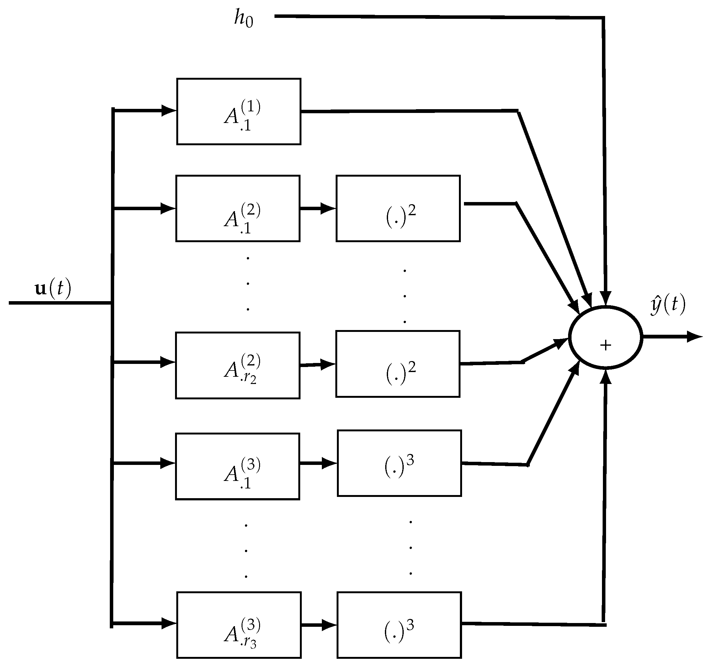
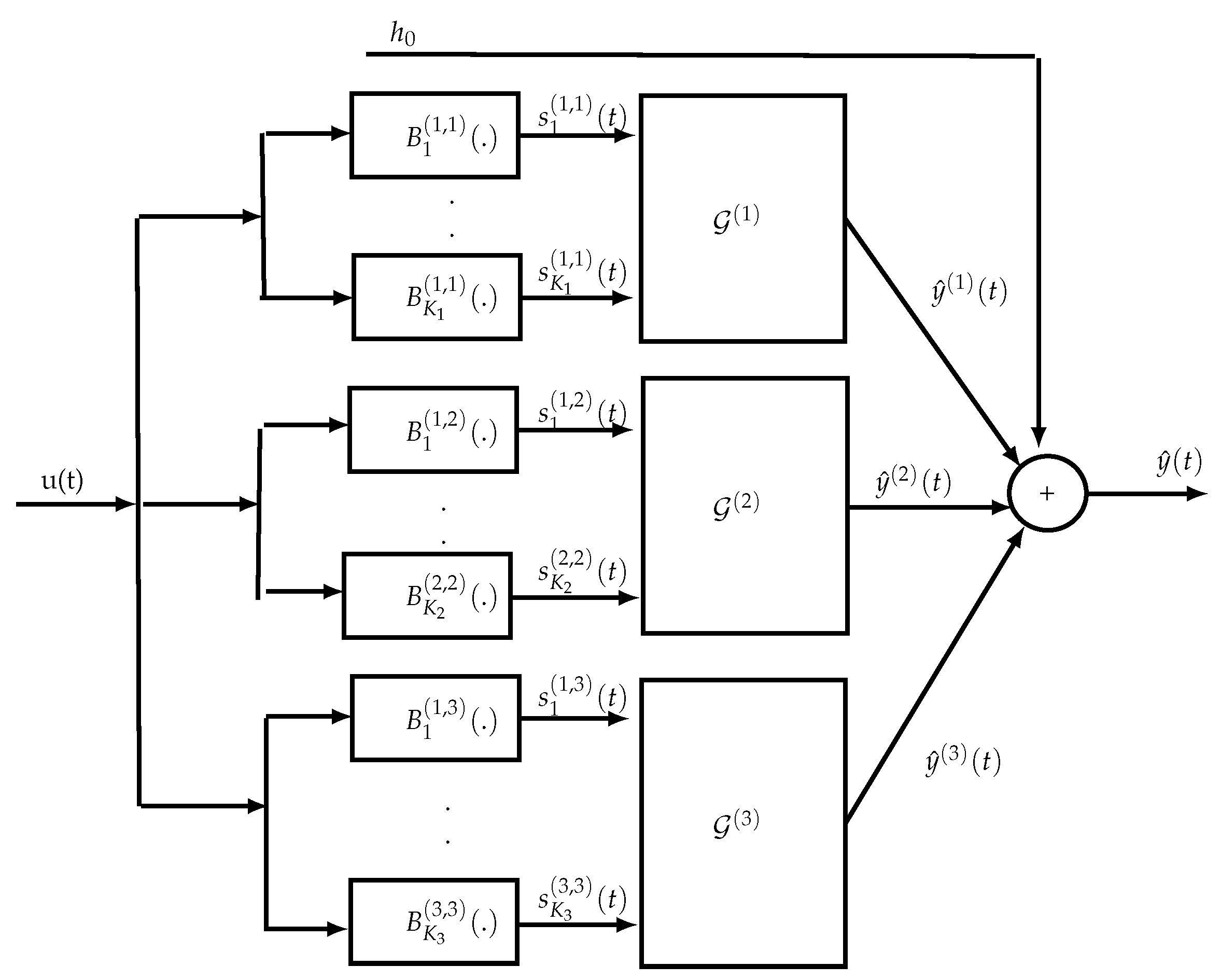
The main drawback of Volterra models is their parametric complexity implying the need to estimate a huge number of parameters which exponentially grows with the order and memory of the kernels. So, several complexity reduction approaches for Volterra models have been developed using symmetrization or triangularization of Volterra kernels, or their expansion on orthogonal bases like Laguerre and Kautz ones, or generalized orthogonal bases (GOB). Considering Volterra kernels as tensors, they can also be decomposed using a PARAFAC decomposition or a tensor train (TT). These approaches lead to the so-called Volterra–Laguerre, Volterra–GOB–Tucker, Volterra–PARAFAC and Volterra–TT models [37,38,39,40,41,42]. In Section 5.3 and Section 5.4, we review the Volterra–PARAFAC and Volterra–GOB–Tucker models. Note that a model-pruning approach can also be employed to adjust the complexity reduction in considering only nearly diagonal coefficients of the kernels and removing the other ones which correspond to more delayed input values whose influence decreases when the delay increases [43].

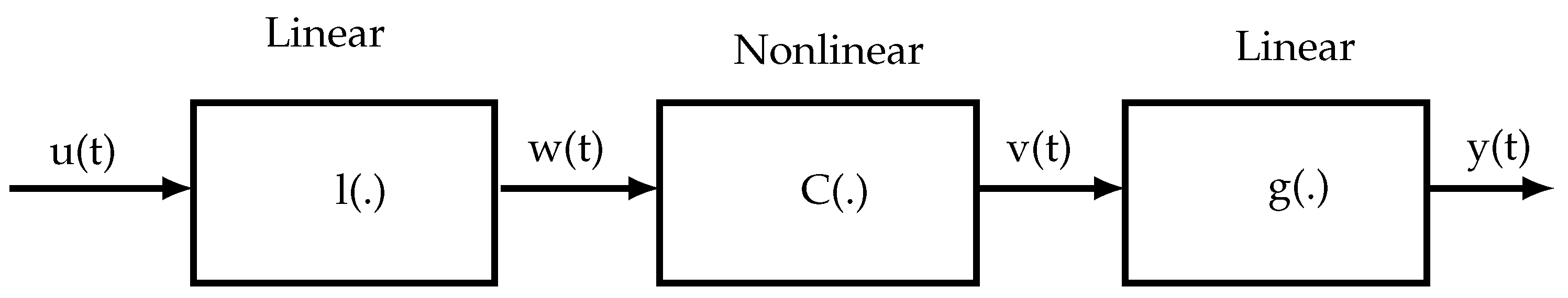
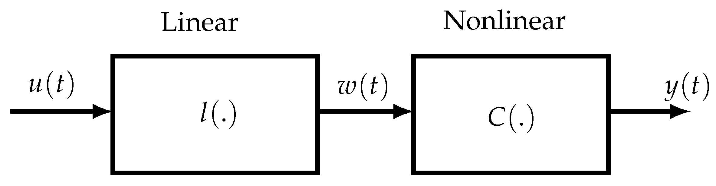
Another approach for ensuring a reduced parametric complexity consists in considering block-oriented NL models, composed of two types of blocks: linear time-invariant (LTI) dynamic blocks and static NL blocks. The linear blocks may be parametric (transfer functions, FIR models, state-space representations) or nonparametric (impulse responses), whereas the NL blocks may be with memory or memoryless. The different blocks are concatenated in series leading to the so-called Hammerstein (NL-LTI) and Wiener (LTI-NL) models, extended to the Wiener–Hammerstein (LTI-NL-LTI) and Hammerstein–Wiener (NL-LTI-NL) models, abbreviated W-H and H-W, respectively. To extend the modeling potential of block-oriented models, several W-H and H-W models can also be interconnected in parallel. Although such models are simpler but less general than Volterra models, they allow us to represent numerous nonlinear systems. One of the first applications of block-oriented NL models was for modeling biological systems [44]. A lot of papers have been devoted to the identification of block-oriented models and their applications. For more details, the reader is referred to the book [45] and the survey papers [46,47].

In Section 5.5, we show that the Wiener, Hammerstein and W-H models are equivalent to structured Volterra models. This equivalence is at the origin of the structure identification method for block-oriented systems, which will be presented in Section 5.5.4. Tensor-based methods using this equivalence have been developed to estimate the parameters of block-oriented nonlinear systems [48,49,50,51]. These methods are generally composed of two steps. In the first one, the Volterra kernel associated with a particular block-oriented system is used to estimate the LTI component(s). Note that there exist closed-form solutions for estimating only the Volterra kernel of interest. Such a solution is proposed in [52,53] for a third-order and fifth-order kernel, respectively. Then, in a second step, the nonlinear block is estimated using the LS method. An example of a tensor-based method for identifying a nonlinear communication channel represented by means of a W-H model was proposed in [54] using the associated third-order Volterra kernel.

On the other hand, multilinear models are useful for modeling coupled dynamical systems in engineering, biology, and physics. Tensor-based approaches have been proposed for solving and identifying multilinear systems [24,55,56]. Using the Einstein product of tensors, we first introduce a new class of systems, the so-called memoryless tensor-input tensor-output (TITO) systems, in which the multidimensional input and output signals define two tensors. The LS method is applied to estimate the tensor transfer of such a system. Then the case of a tensor-input single-output (TISO) system is considered assuming the system transfer is a rank-one Nth-order tensor, which leads to a multilinear system with respect to the impulse responses (IR) of the N subsystems associated with the N modes of the input tensor.

The non-recursive weighted least-squares (WLS) method is used to estimate the multilinear impulse response (MIR) under a vectorized form. A closed-form method is also proposed to estimate the IR of each subsystem from the estimated MIR.

The rest of the paper is structured as follows. In Section 2, we present the notations with the index convention used throughout the paper. In Section 3, we introduce some tensor sets in connection with multilinear forms. In Section 4, we briefly recall basic tensor operations and decompositions. Section 5 and Section 6 are devoted to tensor-based approaches for nonlinear and multilinear systems modeling and identification, respectively. Finally, Section 7 concludes the paper, with some perspectives for future work.

Many books and survey papers discuss estimation theory and system identification. In the field of engineering sciences, we can cite the fundamental contributions of [57,58,59,60,61,62,63] for linear systems and [27,28,29,47,64,65,66,67,68,69] for nonlinear systems. In the case of multilinear systems, the reader is referred to [55,56] for more details.

2. Notation and Index Convention

Scalars, column vectors, matrices, and tensors are denoted by lower-case, boldface lower-case, boldface upper-case, and calligraphic letters, e.g., x, $\mathbf{x}$, X, $\mathcal{X}$, respectively. We denote by $a_{i,r}$ the $(i,r)$ element and by ${\mathbf{A}}_{.r}$ (resp. ${\mathbf{A}}_{i.}$) the rth column (resp. ith row) of $\mathbf{A}\in {\mathbb{C}}^{I\times R}$. ${\mathbf{I}}_R$ denotes the identity matrix of size $R\times R$.

The transpose, complex conjugate, transconjugate, and Moore–Penrose pseudo-inverse operators are represented by ${(.)}^T$, ${(·)}^{*}$, ${(·)}^H$ and ${(·)}^{†}$, respectively.

The operator $\mathrm{diag}(·)$ forms a diagonal matrix from its vector argument, while $D_i\left(\mathbf{A}\right)$ stands for a diagonal matrix holding the ith row of $\mathbf{A}\in {\mathbb{C}}^{I\times R}$ on the diagonal.

The operator ${\mathcal{T}}_{M+N-1,N}(·)$ forms a $(M+N-1)\times N$ Toeplitz matrix from its vector argument $\mathbf{x}\in {\mathbb{C}}^M$, whose first column and row are, respectively, ${\left(\begin{array}{cccc}{x}_1& \cdots & x_M& {\mathbf{0}}_{N-1}^T\end{array}\right)}^T$ and $\left(\begin{array}{cc}{x}_1& {\mathbf{0}}_{N-1}^T\end{array}\right)$.

Given $\mathbf{Y}\in {\mathbb{C}}^{I\times J}$, the vec and unvec operators are defined such that: $\mathbf{y}=\mathrm{vec}\left(\mathbf{Y}\right)\in {\mathbb{C}}^{JI}\leftrightarrow \mathbf{Y}=\mathrm{unvec}\left(\mathbf{y}\right)\in {\mathbb{C}}^{I\times J}$, where the order of dimensions in the product $JI$ is linked to the order of variation of the indices, with the column index j varying more slowly than the row index i.

The outer, Kronecker and Khatri–Rao products are denoted by ∘, ⊗ and ⋄, respectively.

Table 3. Notation for sets of indices and dimensions.

${\underline{\mathbf{i}}}_P\triangleq \{i_1,\cdots ,i_P\}$   ;   ${\underline{\mathbf{j}}}_N\triangleq \{j_1,\cdots ,j_N\}$

${\underline{\mathbf{I}}}_P\triangleq \{I_1,\cdots ,I_P\}$   ;   ${\underline{\mathbf{J}}}_N\triangleq \{J_1,\cdots ,J_N\}$

${\underline{I}}_P\triangleq I_1\times \cdots \times I_P$   ;   ${\underline{J}}_N\triangleq J_1\times \cdots \times J_N$

${\underline{I}}_P\times {\underline{J}}_N=I_1\times \cdots \times I_P\times J_1\times \cdots \times J_N$

${\underline{I}}_P\times {\underline{I}}_P=I_1\times \cdots \times I_P\times I_1\times \cdots \times I_P$

$\mathsf{\Pi }{I}_P\triangleq I_1\cdots I_P={\prod }_{p=1}^P{I}_p$

summarizes the notation used for sets of indices and dimensions [70].

We now introduce the index convention which allows eliminating the summation symbols in formulae involving multi-index variables. For example, ${\sum }_{i=1}^I{a}_i{b}_i$ is simply written as $a_i{b}_i$. Note there are two differences relative to Einstein’s summation convention:

• Each index can be repeated more than twice in an expression;
• Ordered index sets are allowed.

The index convention can be interpreted in terms of two types of summation, the first associated with the row indices (superscripts) and the second associated with the column indices (subscripts), with the following rules [70]:

• The order of the column indices is independent of the order of the row indices;
• Consecutive row and column indices (or index sets) can be permuted.

In

Table 4. Vector and matrix products using the index convention.

$\mathbf{u}\in {\mathbb{K}}^I,\mathbf{v}\in {\mathbb{K}}^J,\mathbf{w}\in {\mathbb{K}}^K$

$\mathbf{u}\otimes \mathbf{v}=u_i{v}_j{\mathbf{e}}_{ij}\in {\mathbb{K}}^{IJ}$

$\mathbf{u}\otimes {\mathbf{v}}^T=u_i{v}_j{\mathbf{e}}_i^j\in {\mathbb{K}}^{I\times J}$

$\mathbf{u}\otimes {\mathbf{v}}^T\otimes \mathbf{w}=u_i{v}_j{w}_k{\mathbf{e}}_{ik}^j\in {\mathbb{K}}^{IK\times J}$

$\mathbf{A}\in {\mathbb{K}}^{I\times J},\mathbf{B}\in {\mathbb{K}}^{J\times K},\mathbf{C}\in {\mathbb{K}}^{K\times J}$

$\mathbf{A}\mathbf{B}={\sum }_{i=1}^I{\sum }_{k=1}^K\left({\sum }_{j=1}^J{a}_{ij}{b}_{jk}\right){\mathbf{e}}_i^k=a_{ij}{b}_{jk}{\mathbf{e}}_i^k\in {\mathbb{K}}^{I\times K}$

$\mathbf{A}{\mathbf{C}}^T=a_{ij}{c}_{kj}{\mathbf{e}}_i^k\in {\mathbb{K}}^{I\times K}$

, we give some examples of vector and matrix products using index convention, where ${\mathbf{e}}_{ij}\triangleq {\mathbf{e}}_i^{\left(I\right)}\otimes {\mathbf{e}}_j^{\left(J\right)},{\mathbf{e}}_i^j\triangleq {\mathbf{e}}_i^{\left(I\right)}\otimes {\left({\mathbf{e}}_j^{\left(J\right)}\right)}^T,{\mathbf{e}}_{ik}^j\triangleq {\mathbf{e}}_i^{\left(I\right)}\otimes {\mathbf{e}}_k^{\left(K\right)}\otimes {\left({\mathbf{e}}_j^{\left(J\right)}\right)}^T$.

Using the index convention, the multiple sum over the indices of $x_{i_1,\cdots ,i_P}{y}_{i_1,\cdots ,i_P}$ will be abbreviated to

$$\sum _{i_1=1}^{I_1}\cdots \sum _{i_P=1}^{I_P}{x}_{i_1,\cdots ,i_P}{y}_{i_1,\cdots ,i_P}=\sum _{{\underline{\mathbf{i}}}_P=\underline{\mathbf{1}}}^{{\underline{\mathbf{I}}}_P}{x}_{{\underline{\mathbf{i}}}_P}{y}_{{\underline{\mathbf{i}}}_P}=x_{{\underline{\mathbf{i}}}_P}{y}_{{\underline{\mathbf{i}}}_P},$$

(1)

where $\underline{\mathbf{1}}$ denotes a set of ones whose number is fixed by the index P of the set ${\underline{\mathbf{I}}}_P$. The notation ${\underline{\mathbf{i}}}_P$ and ${\underline{\mathbf{I}}}_P$ allows us to simplify the expression of the multiple sum into a single sum over an index set, which is further simplified by using the index convention.

3. Tensors and Multilinear Forms

In signal processing applications, a tensor $\mathcal{X}\in {\mathbb{K}}^{I_1\times \cdots \times I_N}$ of order N and size $I_1\times \cdots \times I_N$ is typically viewed as an array of numbers $\left[x_{i_1,\cdots ,i_N}\right]$. The order corresponds to the number of indices $(i_1,\cdots ,i_N)$ that characterize its elements $x_{i_1,\cdots ,i_N}\in \mathbb{K}$, also denoted $x_{i_1\cdots i_N}$ or ${\left(\mathcal{X}\right)}_{i_1,\cdots ,i_N}$. Each index $i_n\in \langle I_n\rangle \triangleq \{1,\cdots ,I_n\}$, for $n\in \langle N\rangle \triangleq \{1,\cdots ,N\}$, is associated with a mode, also called a way, and $I_n$ denotes the dimension of the nth mode. The number of elements in $\mathcal{X}$ is equal to ${\prod }_{n=1}^N{I}_n$. For instance, in a wireless communication system [8], each index of a signal $x_{i_1,\cdots ,i_N}$ corresponds to a different form of diversity (in time, space, frequency, code, etc., domains), and the dimensions $I_n$ are the numbers of time samples, receive antennas, subcarriers, the code length, etc.

The tensor $\mathcal{X}$ is said to be real (resp. complex) if its elements are real numbers (resp. complex numbers), which corresponds to $\mathbb{K}=\mathbb{R}$ (resp. $\mathbb{K}=\mathbb{C}$). It is said to have even order (resp. odd order) if N is even (resp. odd). The special cases $N=2$ and $N=1$ correspond to the sets of matrices $\mathbf{X}\in {\mathbb{K}}^{I\times J}$ and column vectors $\mathbf{x}\in {\mathbb{K}}^I$, respectively.

If $I_1=\cdots =I_N=I$, the Nth-order tensor $\mathcal{X}=\left[x_{i_1,\cdots ,i_N}\right]\in {\mathbb{K}}^{I\times I\times \cdots \times I}$ is said to be hypercubic, of dimensions I, with $i_n\in \langle I\rangle$, for $n\in \langle N\rangle$. The number of elements in $\mathcal{X}$ is then equal to $I^N$. The set of (real or complex) hypercubic tensors of order N and dimensions I will be denoted ${\mathbb{K}}^{[N;I]}$.

A hypercubic tensor of order N and dimensions I is said to be symmetric if it is invariant under any permutation $\pi$ of its modes, i.e.,

$$a_{\pi (i_1,i_2,\cdots ,i_N)}\triangleq a_{i_{\pi \left(1\right)},i_{\pi \left(2\right)},\cdots ,i_{\pi \left(N\right)}}=a_{i_1,i_2,\cdots ,i_N}.$$

(2)

The identity tensor of order N and dimensions I is denoted ${\mathcal{I}}_{N,I}=\left[{\delta }_{i_1,\cdots ,i_N}\right]$, with $i_n\in \langle I\rangle$, for $n\in \langle N\rangle$, or simply $\mathcal{I}$. It is a hypercubic tensor whose elements are defined using the generalized Kronecker delta

$${\delta }_{i_1,\cdots ,i_N}=\left\{\begin{array}{c}1\mathrm{if}{i}_1=\cdots =i_N\hfill \\ 0\mathrm{otherwise}\hfill \end{array}\right..$$

It is a diagonal tensor whose diagonal elements are equal to 1 and other elements to zero, which can be written as the sum of I outer products of N canonical basis vectors ${\mathbf{e}}_i^{\left(I\right)}$ of the space ${\mathbb{R}}^I$

$${\mathcal{I}}_{N,I}=\sum _{i=1}^I\underset{N\mathrm{terms}}{\underbrace{{\mathbf{e}}_i^{\left(I\right)}\circ \cdots \circ {\mathbf{e}}_i^{\left(I\right)}}}.$$

where the outer product operation is defined later in Table 9.

A diagonal tensor $\mathcal{X}\in {\mathbb{K}}^{I\times \cdots \times I}$ of order N, whose diagonal elements are the entries of vector $\mathbf{a}={\left[a_1,\cdots ,a_I\right]}^T$, will be written as

$$x_{i,i_2,\cdots ,i_N}=a_i{\delta }_{i,i_2,\cdots ,i_N}\iff \mathcal{X}=\sum _{i=1}^I{a}_i\underset{N\mathrm{terms}}{\underbrace{{\mathbf{e}}_i^{\left(I\right)}\circ \cdots \circ {\mathbf{e}}_i^{\left(I\right)}}}.$$

Different matricizations, also called matrix unfoldings, can be defined for a tensor $\mathcal{X}\in {\mathbb{K}}^{I_1\times \cdots \times I_N}$. Consider a partitioning of the set of modes $\langle N\rangle$ into two disjoint ordered subsets ${\mathbb{S}}_1$ and ${\mathbb{S}}_2$, composed of p and $N-p$ modes, respectively, with $p\in \langle N-1\rangle$. A general matrix unfolding formula was given by [71] as follows

$${\mathbf{X}}_{{\mathbb{S}}_1;{\mathbb{S}}_2}=\sum _{i_1=1}^{I_1}\cdots \sum _{i_N=1}^{I_N}{x}_{i_1,\cdots ,i_N}\left(\underset{n\in {\mathbb{S}}_1}{\otimes }{\mathbf{e}}_{i_n}^{\left(I_n\right)}\right){\left(\underset{n\in {\mathbb{S}}_2}{\otimes }{\mathbf{e}}_{i_n}^{\left(I_n\right)}\right)}^T\in {\mathbb{K}}^{J_1\times J_2},$$

(3)

where ${\mathbf{e}}_{i_n}^{\left(I_n\right)}$ is the $i_n$-th vector of the canonical basis of ${\mathbb{R}}^{I_n}$, and $J_{n_1}=\underset{n\in {\mathbb{S}}_{n_1}}{\prod I_n}$, for $n_1=1\mathrm{and}2$. We say that ${\mathbf{X}}_{{\mathbb{S}}_1;{\mathbb{S}}_2}$ is a matrix unfolding of $\mathcal{X}$ along the modes of ${\mathbb{S}}_1$ for the rows and along the modes of ${\mathbb{S}}_2$ for the columns, with ${\mathbb{S}}_1\cap {\mathbb{S}}_2=\varnothing$ and ${\mathbb{S}}_1\cup {\mathbb{S}}_2=\langle N\rangle$.

For instance, in the case of a third-order tensor $\mathcal{X}\in {\mathbb{K}}^{I\times J\times K}$, we have six flat unfoldings and six tall unfoldings. For ${\mathbb{S}}_1=1$ and ${\mathbb{S}}_2=\{2,3\}$, we have the following mode-1 flat unfolding ${\mathbf{X}}_{I\times JK}\triangleq {\mathbf{X}}_{1;\{2,3\}}$, while for ${\mathbb{S}}_1=\{2,3\}$ and ${\mathbb{S}}_2=1$ we obtain the following mode-1 tall unfolding ${\mathbf{X}}_{JK\times I}\triangleq {\mathbf{X}}_{\{2,3\};1}={\mathbf{X}}_{I\times JK}^T$.

Vectorized forms of $\mathcal{X}\in {\mathbb{K}}^{I_1\times \cdots \times I_N}$ are obtained by combining the modes in a given order. Thus, a lexicographical vectorization gives the vector $\mathbf{y}\triangleq {\mathbf{x}}_{I_1\cdots I_N}$ with element $x_{i_1,\cdots ,i_N}$ at the position $m=\overline{i_1{i}_2\cdots i_N}$ in $\mathbf{y}$, i.e., $y_m=x_{i_1,\cdots ,i_N}\triangleq x_{{\underline{\mathbf{i}}}_N}$, with [72]

$$\overline{i_1{i}_2\cdots i_N}\triangleq i_N+\sum _{n=1}^{N-1}(i_n-1)\prod _{k=n+1}^N{I}_k.$$

(4)

By convention, the order of the dimensions in a product ${\prod }_{n=1}^N{I}_n\triangleq I_1\cdots I_N$ associated with the index combination $\overline{i_1{i}_2\cdots i_N}$ follows the order of variation of the indices $(i_1,\cdots ,i_N)$, with $i_1$ varying more slowly than $i_2$, which in turn varies more slowly than $i_3$, etc.

The Frobenius norm of $\mathcal{X}\in {\mathbb{K}}^{I_1\times \cdots \times I_N}$ is the square root of the inner product of the tensor with itself, i.e.,

$${\parallel \mathcal{X}\parallel }_F=\sqrt{\langle \mathcal{X},\mathcal{X}\rangle }={\left(\sum _{i_1=1}^{I_1}\cdots \sum _{i_N=1}^{I_N}{\left|x_{i_1,\cdots ,i_N}\right|}^2\right)}^{1/2}.$$

(5)

Table 5. Various sets of tensors.

Order	Size	Sets of Tensors
P	${\underline{I}}_P=I_1\times \cdots \times I_P$	${\mathbb{K}}^{I_1\times \cdots \times I_P}\triangleq {\mathbb{K}}^{{\underline{I}}_P}$
P	${\underline{I}}_P=I_1\times \cdots \times I_P\mathrm{with}{I}_p=I,\forall p\in \langle P\rangle$	${\mathbb{K}}^{[P;I]}$
$P+N$	${\underline{I}}_P\times {\underline{J}}_N=I_1\times \cdots \times I_P\times J_1\times \cdots \times J_N$	${\mathbb{K}}^{{\underline{I}}_P\times {\underline{J}}_N}$
	${\underline{I}}_P\times {\underline{J}}_N=I\times \cdots \times I\times J\times \cdots \times J$
$P+N$	with	${\mathbb{K}}^{[P+N;I,J]}$
	$I_p=I,\forall p\in \langle P\rangle$   and   $J_n=J,\forall n\in \langle N\rangle$
$2P$	${\underline{I}}_P\times {\underline{I}}_P$   with   $I_p=I,\forall p\in \langle P\rangle$	${\mathbb{K}}^{[2P;I]}$

presents various sets of tensors that will be considered in this paper, with the notation introduced in [70].

We can make the following remarks about the sets of tensors defined in Table 5:

•

For $P=N=1$, the set ${\mathbb{K}}^{[2;I,J]}$ is the set ${\mathbb{K}}^{I\times J}$ of (real or complex) matrices of size $I\times J$.

•

The set ${\mathbb{K}}^{[P;I]}$ is also denoted ${{\mathbb{K}}^I}^P$ or T${}^P\left(K^I\right)$ by some authors.

•

The set ${\mathbb{K}}^{{\underline{I}}_P\times {\underline{I}}_P}$ is called the set of even-order (or square) tensors of order $2P$ and size ${\underline{I}}_P\times {\underline{I}}_P$. The name of square tensor comes from the fact that the index set is divided into two identical subsets of dimension ${\underline{I}}_P$.

•

Analogously to matrices, tensors in the sets ${\mathbb{K}}^{{\underline{I}}_P\times {\underline{J}}_P}$ with $J_p\ne I_p$ and ${\mathbb{K}}^{{\underline{I}}_P\times {\underline{J}}_N}$ are said to be rectangular. The set ${\mathbb{K}}^{{\underline{I}}_P\times {\underline{J}}_N}$ is called the set of rectangular tensors with index blocks of dimensions ${\underline{I}}_P$ and ${\underline{J}}_N$.

The various tensor sets introduced above can be associated with scalar real-valued multilinear forms in vector variables and with homogeneous polynomials. Like in the matrix case, we will distinguish between homogeneous polynomials of degree P that depend on the components of P vector variables and those that depend on just one vector variable.

A real-valued multilinear form, also called a P-linear form, is a map f such as

$$\stackrel{P}{\underset{p=1}{\times }}{\mathbb{R}}^{I_p}\ni ({\mathbf{x}}^{\left(1\right)},\cdots {\mathbf{x}}^{\left(P\right)})⟼f\left({\mathbf{x}}^{\left(1\right)},\cdots {\mathbf{x}}^{\left(P\right)}\right)\in \mathbb{R}$$

(6)

that is separately linear with respect to each vector variable ${\mathbf{x}}^{\left(p\right)}$ when the other variables ${\mathbf{x}}^{\left(q\right)}$, for $q\ne p$, are fixed. Using the index convention, the multilinear form can be written for ${\mathbf{x}}^{\left(p\right)}\in {\mathbb{R}}^{I_p}$, $p\in \langle P\rangle$, as

$$f\left({\mathbf{x}}^{\left(1\right)},\cdots ,{\mathbf{x}}^{\left(P\right)}\right)=\sum _{i_1=1}^{I_1}\cdots \sum _{i_P=1}^{I_P}{a}_{i_1,\cdots ,i_P}{x}_{i_1}^{\left(1\right)}\cdots x_{i_P}^{\left(P\right)}=a_{{\underline{\mathbf{i}}}_P}\prod _{p=1}^P{x}_{i_p}^{\left(p\right)}.$$

(7)

The tensor $\mathcal{A}\in {\mathbb{R}}^{{\underline{I}}_P}$ is called the tensor associated with the multilinear form f.

Two multilinear forms are presented in

Table 6. Multilinear forms and associated tensors.

Multilin. Forms	Transformations	Tensors
real-valued in P vectors	$\stackrel{P}{\underset{p=1}{\times }}{\mathbb{R}}^{I_p}\ni ({\mathbf{x}}^{\left(1\right)},\cdots {\mathbf{x}}^{\left(P\right)})⟼f\left({\mathbf{x}}^{\left(1\right)},\cdots {\mathbf{x}}^{\left(P\right)}\right)\in \mathbb{R}$	$\mathcal{A}\in {\mathbb{R}}^{{\underline{I}}_P}$
real-valued in one vector	${\mathbb{R}}^I\ni \mathbf{x}⟼f\underset{P\mathrm{terms}}{\underbrace{(\mathbf{x},\cdots ,\mathbf{x})}}\in \mathbb{R}$	$\mathcal{A}\in {\mathbb{R}}^{[P;I]}$

, which also states the transformation corresponding to each of them, as well as the associated tensor.

Table 7. Multilinear forms and associated homogeneous polynomials.

Forms	Matrices/Tensors	Homogeneous Polynomials
Bilinear	$\mathbf{A}\in {\mathbb{R}}^{I\times J};\mathbf{y}\in {\mathbb{R}}^I,\mathbf{x}\in {\mathbb{R}}^J$	$f(\mathbf{x},\mathbf{y})={\mathbf{y}}^T\mathbf{A}\mathbf{x}=a_{ij}{y}_i{x}_j,i\in \langle I\rangle ,j\in \langle J\rangle$
Quadratic	$\mathbf{A}\in {\mathbb{R}}^{I\times I};\mathbf{x}\in {\mathbb{R}}^I$	$f\left(\mathbf{x}\right)={\mathbf{x}}^T\mathbf{A}\mathbf{x}=a_{ij}{x}_i{x}_j,i,j\in \langle I\rangle$
Real multilinear in P vector	$\mathcal{A}\in {\mathbb{R}}^{{\underline{I}}_P};{\mathbf{x}}^{\left(p\right)}\in {\mathbb{R}}^{I_p}$	$f\left({\mathbf{x}}^{\left(1\right)},\cdots {\mathbf{x}}^{\left(P\right)}\right)=a_{{\underline{\mathbf{i}}}_P}{\prod }_{p=1}^P{x}_{i_p}^{\left(p\right)},i_p\in \langle I_p\rangle ,p\in \langle P\rangle$
Real multilinear in one vector	$\mathcal{A}\in {\mathbb{R}}^{[P;I]};\mathbf{x}\in {\mathbb{R}}^I$	$f\underset{P\mathrm{terms}}{\underbrace{(\mathbf{x},\cdots ,\mathbf{x})}}=a_{{\underline{\mathbf{i}}}_P}{\prod }_{p=1}^P{x_i}_p,i_p\in \langle I\rangle ,p\in \langle P\rangle$

recalls the definitions of bilinear/quadratic forms using the index convention, then presents the multilinear forms defined in Table 6, as well as the associated tensors from Table 5 and the corresponding homogeneous polynomials.

We can make the following remarks:

• In the same way that bilinear forms depend on two variables that do not necessarily belong to the same vector space, general real multilinear forms depend on P variables that may belong to different vector spaces: ${\mathbf{x}}^{\left(p\right)}\in {\mathbb{R}}^{I_p}$.
• Analogously to quadratic forms obtained from bilinear forms by replacing the pair $(\mathbf{x},\mathbf{y})$ with the vector $\mathbf{x}$, real multilinear forms can be expressed using just one vector $\mathbf{x}\in {\mathbb{K}}^I$. In the same way symmetric quadratic forms lead to the notion of symmetric matrices, the symmetry of multilinear forms is directly linked to the symmetry of their associated tensors.

4. Tensor Operations and Decompositions

In Section 4.1, we introduce different multiplications with tensors. Then, in Section 4.2, we present the two most used tensor decompositions, namely the PARAFAC (parallel factors) and Tucker decompositions [12,13].

For a more in-depth presentation of tensor tools, the reader is referred to the recent book [70] and review papers [73,74].

4.1. Multiplications with Tensors

In

Table 8. Different types of multiplication with tensors.

Tensors	Operations	Definitions
$\mathcal{X}\in {\mathbb{K}}^{{\underline{I}}_P},\mathbf{A}\in {\mathbb{K}}^{J\times I_p}$	$\mathcal{Y}=\mathcal{X}{\times }_p\mathbf{A}$	$y_{i_1,\cdots ,i_{p-1},j,i_{p+1},\cdots ,i_P}={\sum }_{i_p}{a}_{j,i_p}{x}_{{\underline{\mathbf{i}}}_P}=a_{j,i_p}{x}_{{\underline{\mathbf{i}}}_P}$
$\mathcal{X}\in {\mathbb{K}}^{{\underline{I}}_P},\mathbf{u}\in {\mathbb{K}}^{I_p}$	$\mathcal{Y}=\mathcal{X}{\times }_p{\mathbf{u}}^T$	$y_{i_1,\cdots ,i_{p-1},i_p,\cdots ,i_P}={\sum }_{i_p}{u}_{i_p}{x}_{{\underline{\mathbf{i}}}_P}=u_{i_p}{x}_{{\underline{\mathbf{i}}}_P}$
$\mathcal{X}\in {\mathbb{K}}^{{\underline{I}}_P},\mathcal{Y}\in {\mathbb{K}}^{{\underline{J}}_N}$	$\mathcal{Z}=\mathcal{X}{\times }_p^n\mathcal{Y}$	$z_{i_1,\cdots ,i_{p-1},i_{p+1},\cdots ,i_P,j_1,\cdots ,j_{n-1},j_{n+1},\cdots ,j_N}=$
with   $I_p=J_n=K$		${\sum }_{k=1}^K{a}_{i_1,\cdots ,i_{p-1},k,i_{p+1},\cdots ,i_P}{b}_{j_1,\cdots ,j_{n-1},k,j_{n+1},\cdots ,j_N}$
$\mathcal{A}\in {\mathbb{K}}^{{\underline{I}}_P\times {\underline{J}}_N},\mathcal{X}\in {\mathbb{K}}^{{\underline{J}}_N\times {\underline{K}}_Q}$	$\mathcal{Y}=\mathcal{A}{★}_N\mathcal{X}$	$y_{{\underline{\mathbf{i}}}_P,{\underline{\mathbf{k}}}_Q}={\displaystyle \sum _{{\underline{\mathbf{j}}}_N=\underline{\mathbf{1}}}^{{\underline{\mathbf{J}}}_N}}{a}_{{\underline{\mathbf{i}}}_P,{\underline{\mathbf{j}}}_N}{x}_{{\underline{\mathbf{j}}}_N,{\underline{\mathbf{k}}}_Q}=a_{{\underline{\mathbf{i}}}_P,{\underline{\mathbf{j}}}_N}{x}_{{\underline{\mathbf{j}}}_N,{\underline{\mathbf{k}}}_Q}$

, we present three types of multiplication with tensors, using the notation of Table 3 and the index convention: mode-p, mode-$(p,n)$, and Einstein products.

The multiplication ${\times }_p$, called mode-p or Tucker product, corresponds to a summation over the index $i_p$ associated with the mode p of the Pth-order tensor $\mathcal{X}$ and the second index of $\mathbf{A}$, giving a tensor of order $P-1$, and size $I_1\times \cdots \times I_{p-1}\times I_{p+1}\times \cdots \times I_P$.

The mode-$(p,n)$ product, denoted ${\times }_p^n$, corresponds to a contraction operation performed for two arbitrary modes $(p,n)$, such as: $I_p=J_n=K$. This multiplication gives a tensor of order $P+N-2$ and size $I_1\times \cdots \times I_{p-1}\times I_{p+1}\times \cdots \times I_P\times J_1\times \cdots \times J_{n-1}\times J_{n+1}\times \cdots \times J_N$.

The Einstein product, denoted $\mathcal{A}{★}_N\mathcal{X}$, of the tensors $\mathcal{A}\in {\mathbb{K}}^{{\underline{I}}_P\times {\underline{J}}_N}$ of order $P+N$ and $\mathcal{X}\in {\mathbb{K}}^{{\underline{J}}_N\times {\underline{K}}_Q}$ of order $N+Q$ corresponds to a contraction along the N shared indices ${\underline{\mathbf{j}}}_N$, associated with the N last modes of $\mathcal{A}$ and the N first modes of $\mathcal{X}$. The tensor $\mathcal{A}$ can be interpreted as a multilinear operator associated with a multilinear transformation applied to the tensor $\mathcal{X}$. The Einstein product will be used in Section 6 for defining multilinear systems.

Table 9. Outer products of vectors, matrices, and tensors.

Vectors/Matrices/Tensors	Outer Products	Spaces	Orders
${\mathbf{u}}^{\left(p\right)}\in {\mathbb{K}}^{I_p}$, $p\in \langle P\rangle$	$\stackrel{P}{\underset{p=1}{\circ }}{\mathbf{u}}^{\left(p\right)}$	${\mathbb{K}}^{{\underline{I}}_P}$	P
${\mathbf{A}}^{\left(p\right)}\in {\mathbb{K}}^{I_p\times J_p},p\in \langle P\rangle$	$\stackrel{P}{\underset{p=1}{\circ }}{\mathbf{A}}^{\left(p\right)}$	${\mathbb{K}}^{I_1\times J_1\times \cdots \times I_P\times J_P}$	$2P$
$\mathcal{A}\in {\mathbb{K}}^{{\underline{I}}_P},\mathcal{B}\in {\mathbb{K}}^{{\underline{J}}_N}$	$\mathcal{A}\circ \mathcal{B}$	${\mathbb{K}}^{{\underline{I}}_P\times {\underline{J}}_N}$	$P+N$
${\mathcal{A}}^{\left(p\right)}\in {\mathbb{K}}^{{\underline{J}}_{N_p}},p\in \langle P\rangle$	$\stackrel{P}{\underset{p=1}{\circ }}{\mathcal{A}}^{\left(p\right)}$	${\mathbb{K}}^{{\underline{J}}_{N_1}\times \cdots \times {\underline{J}}_{N_P}}$	${\sum }_{p=1}^P{N}_p$

presents a few examples of outer products of vectors, matrices, and tensors, indicating the order and the space to which the tensors resulting from the products belong.

4.2. PARAFAC and Tucker Decompositions

The PARAFAC decomposition [13] is also called CANDECOMP (canonical decomposition) by [75] and CP for CANDECOMP/PARAFAC by [76] when applied to decompose a data tensor. In the context of system modeling, it is called a PARAFAC model. It amounts to decomposing a tensor into a sum of R polyads, i.e., R rank-one tensors [10]. For an Nth-order tensor $\mathcal{X}$, each polyad corresponds to the outer product of the rth columns of N factor matrices ${\mathbf{A}}^{\left(n\right)}\in {\mathbb{K}}^{I_n\times R}$, i.e., $\stackrel{N}{\underset{n=1}{\circ }}{\mathbf{A}}_{.r}^{\left(n\right)}$. When R is minimal, it is called the tensor rank or canonical rank of $\mathcal{X}$. PARAFAC is also called a canonical polyadic decomposition (CPD), and concisely written as $\{{\mathbf{A}}^{\left(1\right)},\cdots ,{\mathbf{A}}^{\left(N\right)};R\}$. When $R=1$, $\mathcal{X}\in {\mathbb{K}}^{{\underline{I}}_N}$ is a rank-one tensor, also called a separable tensor. Then, it can be written as the outer product of N non-zero vectors ${\mathbf{a}}^{\left(n\right)}\in {\mathbb{K}}^{I_n}$

$$\mathcal{X}=\stackrel{N}{\underset{n=1}{\circ }}{\mathbf{a}}^{\left(n\right)}⟺x_{{\underline{\mathbf{i}}}_N}=\prod _{n=1}^N{a}_{i_n}^{\left(n\right)}.$$

(8)

In the case of a symmetric rank-one tensor $\mathcal{X}\in {\mathbb{K}}^{[N,I]}$, all the vectors ${\mathbf{a}}^{\left(n\right)}\in {\mathbb{K}}^I$ are identical [77].

In

Table 10. PARAFAC decomposition of a tensor of order three and order N.

Third-Order Tensor		Nth-Order Tensor
$\mathcal{X}\in {\mathbb{K}}^{I\times J\times K}$		$\mathcal{X}\in {\mathbb{K}}^{{\underline{I}}_N}$
$\mathbf{A}\in {\mathbb{K}}^{I\times R},\mathbf{B}\in {\mathbb{K}}^{J\times R},\mathbf{C}\in {\mathbb{K}}^{K\times R},$		${\mathbf{A}}^{\left(n\right)}\in {\mathbb{K}}^{I_n\times R}$
$x_{i,j,k}={\displaystyle \sum _{r=1}^R}{a}_{ir}{b}_{jr}{c}_{kr}$	Scalar writing	$x_{{\underline{i}}_N}={\displaystyle \sum _{r=1}^R}{\displaystyle \prod _{n=1}^N}{a}_{i_n,r}^{\left(n\right)}$
$\mathcal{X}={\mathcal{I}}_R{\times }_1\mathbf{A}{\times }_2\mathbf{B}{\times }_3\mathbf{C}$	with mode-n products	$\mathcal{X}={\mathcal{I}}_R\stackrel{N}{\underset{n=1}{\times }}{\mathbf{A}}^{\left(n\right)}$
$\mathcal{X}={\displaystyle \sum _{r=1}^R}{\mathbf{A}}_{.r}\circ {\mathbf{B}}_{.r}\circ {\mathbf{C}}_{.r}$	with outer products	$\mathcal{X}={\displaystyle \sum _{r=1}^R}\stackrel{N}{\underset{n=1}{\circ }}{\mathbf{A}}_{.r}^{\left(n\right)}$
${\mathbf{X}}_{IJ\times K}=(\mathbf{A}\diamond \mathbf{B}){\mathbf{C}}^T$	Matrix unfoldings	${\mathcal{X}}_{{\mathbb{S}}_1;{\mathbb{S}}_2}=\left(\underset{n\in {\mathbb{S}}_1}{\diamond }{\mathbf{A}}^{\left(n\right)}\right){\left(\underset{n\in {\mathbb{S}}_2}{\diamond }{\mathbf{A}}^{\left(n\right)}\right)}^T$
${\mathbf{X}}_{JK\times I}=(\mathbf{B}\diamond \mathbf{C}){\mathbf{A}}^T$
${\mathbf{X}}_{KI\times J}=(\mathbf{C}\diamond \mathbf{A}){\mathbf{B}}^T$
$x_{IJK}=(\mathbf{A}\diamond \mathbf{B}\diamond \mathbf{C})1_R$	Vectorized form	${\mathbf{x}}_{I_1·I_N}=({\mathbf{A}}^{\left(1\right)}\diamond {\mathbf{A}}^{\left(2\right)}\diamond \cdots \diamond {\mathbf{A}}^{\left(N\right)}){\mathbf{1}}_R$

, we present different ways of writing a PARAFAC decomposition for a third-order and Nth-order tensor: scalar writing, with mode-p and outer products, and matrix unfoldings as defined in (3).

PARAFAC models have the following two main features:

• Essential uniqueness, i.e., uniqueness up to trivial indeterminacies corresponding to permutation and scalar ambiguities of the columns of the factor matrices (see [78,79]);
• Existence of a simple algorithm, the so-called alternating least-squares (ALS), for estimating the PARAFAC parameters for a tensor of an arbitrary order N.

The Tucker decomposition [12] of a tensor $\mathcal{X}\in {\mathbb{K}}^{{\underline{I}}_N}$ can be viewed as a generalization of the PARAFAC decomposition in the sense that such a decomposition allows taking into account all interactions between distinct columns of the factor matrices ${\mathbf{A}}^{\left(n\right)}\in {\mathbb{K}}^{I_n\times R_n}$, when a PARAFAC model only involves interactions between the same columns $r\in \langle R\rangle$ of the factor matrices ${\mathbf{A}}^{\left(n\right)}\in {\mathbb{K}}^{I_n\times R}$. In

Table 11. Tucker decomposition of a tensor of order three and order N.

Third-Order Tensor		Nth-Order Tensor
$\mathcal{X}\in {\mathbb{K}}^{I\times J\times K}$		$\mathcal{X}\in {\mathbb{K}}^{{\underline{I}}_N}$
$\mathcal{G}\in {\mathbb{K}}^{P\times Q\times S}$, $\mathbf{A}\in {\mathbb{K}}^{I\times P}$,		$\mathcal{G}\in {\mathbb{K}}^{{\underline{R}}_N}$, ${\mathbf{A}}^{\left(n\right)}\in {\mathbb{K}}^{I_n\times R_n},n\in \langle N\rangle$
$\mathbf{B}\in {\mathbb{K}}^{J\times Q},\mathbf{C}\in {\mathbb{K}}^{K\times S}$
$x_{ijk}={\displaystyle \sum _{p=1}^P}{\displaystyle \sum _{q=1}^Q}{\displaystyle \sum _{s=1}^S}{g}_{pqs}{a}_{ip}{b}_{jq}{c}_{ks}$	Scalar writing	$x_{{\underline{i}}_N}={\displaystyle \sum _{r_1=1}^{R_1}}\cdots {\displaystyle \sum _{r_N=1}^{R_N}}{g}_{r_1,\cdots ,r_N}{\prod }_{n=1}^N{a}_{i_n,r_n}^{\left(n\right)}$
$\mathcal{X}=\mathcal{G}{\times }_1\mathbf{A}{\times }_2\mathbf{B}{\times }_3\mathbf{C}$	with mode-n products	$\mathcal{X}=\mathcal{G}{\times }_1{\mathbf{A}}^{\left(1\right)}{\times }_2{\mathbf{A}}^{\left(2\right)}{\times }_3\cdots {\times }_N{\mathbf{A}}^{\left(N\right)}$
$\mathcal{X}={\displaystyle \sum _{p=1}^P}{\displaystyle \sum _{q=1}^Q}{\displaystyle \sum _{s=1}^S}{g}_{pqs}{\mathbf{A}}_{.p}\circ {\mathbf{B}}_{.q}\circ {\mathbf{C}}_{.s}$	with outer products	$\mathcal{X}={\displaystyle \sum _{r_1=1}^{R_1}}\cdots {\displaystyle \sum _{r_N=1}^{R_N}}{g}_{r_1,\cdots ,r_N}\stackrel{N}{\underset{n=1}{\circ }}{\mathbf{A}}_{.r_n}^{\left(n\right)}$

, we present different ways of writing a Tucker decomposition for a third-order and Nth-order tensor. From the writing with outer products, we can conclude that the Tucker model of a Nth-order tensor consists in a weighted sum of ${\prod }_{n=1}^N{R}_n$ rank-one tensors, where the coefficients $g_{r_1,\cdots ,r_N}$ of the core tensor $\mathcal{G}\in {\mathbb{K}}^{{\underline{R}}_N}$, define the weights of the interactions between the columns ${\mathbf{A}}_{.r_n}^{\left(n\right)}$ of the factor matrices.

Note that a Tucker decomposition is generally not essentially unique, unless additional constraints are imposed, such as a perfect knowledge of the core tensor, certain sparseness or structural constraints on the core tensor or the matrix factors [80,81]. Consult [82] for a review of uniqueness results for Tucker models.

5. Tensor-Based Approaches for Nonlinear Systems

The use of tensor-based approaches for nonlinear systems has proved advantageous in three areas: (i) parametric complexity reduction in order to get efficient and computationally fast parameters estimation algorithms, (ii) generating new representations of nonlinear systems thanks to tensor decompositions, and (iii) structural identification of systems which can be represented as combinations of dynamical linear systems with static nonlinear blocks. In Section 5.1, we first describe polynomial models. Then, in Section 5.2, we introduce standard discrete-time Volterra models. To reduce the parametric complexity of such models, in Section 5.3, we present a tensor approach which consists in using a PARAFAC decomposition of Volterra kernels. The expansion of Volterra kernels on orthogonal bases is considered in Section 5.4. Finally, some links between block-oriented models (Hammerstein, Wiener, and Wiener–Hammerstein) and tensor representations via their associated Volterra kernels are established in Section 5.5

5.1. Polynomial Models

Polynomial models are a direct extension of linear models. For a single-input single-output (SISO) system, the output of a recursive polynomial model, at discrete-time instant t, is given by

$$\widehat{y}\left(t\right)=\sum _{p=1}^P{f}_p[u\left(t\right),\cdots ,u(t-n_u),y(t-1),\cdots ,y(t-n_y)],$$

(9)

where $f_p(.)$ is a pth-degree polynomial in the system input $\left(u\right)$ and output $\left(y\right)$ signals, P is the nonlinearity order, and $M=max(n_u,n_y)$ is the memory of the model. In the sequel, all the signals will be assumed to be real-valued.

The input/output (I/O) relationship (9) is also called a nonlinear autoregressive with exogenous input (NARX) model [83], or a one-step prediction model, i.e., a model whose output $\widehat{y}\left(t\right)$ at time t depends on past values $y(t-n)$ (for $n\in \langle n_y\rangle$) of the system output, and current and past values $u(t-n)$ (for $n=0,1,\cdots ,n_u$) of the system input. This model is an extension of the standard autoregressive with exogenous input (ARX) model, frequently used to study discrete time series, due to the presence of nonlinear terms in the input–output signals, which explains its success in many industrial applications.

Equation (9) can also be written as a regression model which is linear in its parameters, namely the polynomial coefficients, and nonlinear in the I/O signals:

$$\widehat{y}\left(t\right)={\mathit{\phi }}^T(\mathbf{u}\left(t\right),\mathbf{y}(t-1))\mathit{\theta },$$

(10)

where $\mathbf{u}\left(t\right)={[u\left(t\right)\cdots u(t-n_u)]}^T$, $\mathbf{y}(t-1)={[y(t-1)\cdots y(t-n_y)]}^T$, and $\mathit{\phi }$ is the nonlinear regressor vector whose components are monomials in (i.e., products of) previous system outputs and previous and current system inputs contained in the vectors $\mathbf{y}(t-1)$ and $\mathbf{u}\left(t\right)$, and $\mathit{\theta }$ is the parameter vector containing the polynomial coefficients.

If the previous system outputs $y(t-1),\cdots ,y(t-n_y)$ are replaced by previous model outputs $\widehat{y}(t-1),\cdots ,\widehat{y}(t-n_y)$, the polynomial model (9) is then called a simulation or nonlinear output error (NOE) model, defined as

$$\widehat{y}\left(t\right)=\sum _{p=1}^P{f}_p[u\left(t\right),\cdots ,u(t-n_u),\widehat{y}(t-1),\cdots ,\widehat{y}(t-n_y)]={\mathit{\phi }}^T(\mathbf{u}\left(t\right),\widehat{\mathbf{y}}(t-1))\mathit{\theta },$$

(11)

with $\widehat{\mathbf{y}}(t-1)={[\widehat{y}(t-1)\cdots \widehat{y}(t-n_y)]}^T$.

This model is recursive with respect to previous model outputs $\widehat{y}(t-n)$ (for $n\in \langle n_y\rangle$), while the one-step prediction model (10) is purely feedforward.

As for linear systems, the advantage of NARX and NOE models with output feedback is to be more parsimonious than without output feedback, which means a reduced parametric complexity in terms of dimension of the parameter vector $\mathit{\theta }$. One drawback of output feedback is that stability is generally not guaranteed. Another drawback of NOE models is that they need to use a nonlinear optimization method for parameter estimation due to the dependence of $\widehat{\mathbf{y}}(t-1)$ on $\mathit{\theta }$ in the regression Equation (11) implying a nonlinear dependence of the model output with respect to model parameters. That is not the case for the NARX model that is linear in its parameters, whose estimation can therefore be carried out by means of the standard least-squares (LS) algorithm.

5.2. Truncated Volterra Models

When the polynomial functions $f_p(.)$ in (9) are independent from the output signal, i.e., without output feedback, the polynomial model is called a nonrecursive polynomial model or a discrete-time Volterra model. A Pth-order Volterra model for a causal, stable, finite-memory, time-invariant SISO system is described by the following I/O relationship:

$$\widehat{\mathbf{y}}\left(t\right)=h_0+\sum _{p=1}^P\sum _{m_1=1}^{M_p}\cdots \sum _{m_P=1}^{M_P}{h}_{m_1,\cdots ,m_P}^{\left(p\right)}\prod _{q=1}^{p}u(t-m_q+1)=h_0+\sum _{p=1}^P{\widehat{y}}^{\left(p\right)}\left(t\right),$$

(12)

where $h_0$ is the offset, $M_p$ is the memory of the pth-order homogeneous term ${\widehat{y}}^{\left(p\right)}\left(t\right)$, and $h_{m_1,\cdots ,m_P}^{\left(p\right)}$ is a coefficient of the pth-order Volterra kernel, assumed to be real-valued.

Note that a truncated Volterra model can be seen as a truncated Taylor series expansion for approximating a given smooth nonlinear function (around 0 by convention).

Equation (12) can also be written as a polynomial regression model linear in its parameters and composed of monomials in previous samples of the input signal

$$\widehat{\mathbf{y}}\left(t\right)=h_0+{\mathit{\phi }}^T\left(\mathbf{u}\left(t\right)\right)\mathit{\theta },$$

(13)

where $\mathbf{u}\left(t\right)={[u\left(t\right),\cdots ,u(t-M)]}^T$, with $M=ma{x}_p\left(M_p\right)$, and $\mathit{\theta }$ is the parameter vector containing all the kernel coefficients, and the vector $\mathit{\phi }$ contains all possible monomials in u up to degree P. In the sequel, we assume that all memories $M_p$ are equal to M. The coefficient $h_{m_1,\cdots ,m_P}^{\left(p\right)}$ being characterized by p indices can be viewed as an element of a tensor ${\mathcal{H}}^{\left(p\right)}\in {\mathbb{R}}^{[p,M]}$, of order p, characterized by $M^p$ entries, which is a number growing very fast with the kernel order p. The pth-order homogeneous term ${\widehat{y}}^{\left(p\right)}\left(t\right)$ can then be written using the Tucker product as

$${\widehat{y}}^{\left(p\right)}\left(t\right)={\mathcal{H}}^{\left(p\right)}\stackrel{p}{\underset{q=1}{\times }}{\mathbf{u}}^T\left(t\right),$$

(14)

which is a homogeneous polynomial of degree p in the components of the input vector.

Several adaptive and nonadaptive methods have been proposed to identify truncated Volterra models from I/O measurements, both in the time and frequency domains. Frequency methods are based on the use of input signal cumulants, which requires estimating high-order statistics of the input signal, up to order $2P$ for a Pth-order Volterra model. Such an approach is mainly interesting with a Gaussian input signal, since the input cumulants of order higher than two are then zero, which implies a significant simplification of frequency methods. In the time domain, we can distinguish the optimal minimum mean-square error (MMSE) estimator, based on the use of input signal statistics, the nonrecursive least-squares (LS) algorithm, which can be viewed as an approximation of the MMSE solution, and adaptive methods. Note that estimating the parameters of an homogeneous Pth-order Volterra kernel, with memory M, using the MMSE and nonrecursive LS solutions requires inverting an autocorrelation matrix of size $M^P\times M^P$, which is a time consuming and numerically difficult task.

Adaptive methods are often associated with adaptive Volterra filters used for representing NL time-varying signals and systems as encountered in echo cancellation, for instance. Parameter estimation of adaptive Volterra filters is carried out using the well-known least-mean-square (LMS) or recursive LS (RLS) algorithms. See the book [28] and the references therein for an overview of the methods briefly introduced above.

In the next section, we present an approach for identifying reduced complexity Volterra models which is based on a PARAFAC decomposition of symmetrized kernels, leading to the so-called Volterra–PARAFAC models.

5.3. Volterra–PARAFAC Models

As each permutation of the indices $m_1,\cdots ,m_p$ corresponds to the same product ${\prod }_{q=1}^{p}u(t-m_q+1)$ of delayed inputs, we can sum all the coefficients associated with these permutations to get a symmetric kernel given by

$$h_{m_1,\cdots ,m_P}^{(p,sym)}=\frac{1}{p!}\sum _{\pi (.)}{h}_{m_{\pi \left(1\right)},\cdots ,m_{\pi \left(p\right)}}^{\left(p\right)},$$

where $\left(\pi \right(1),\cdots ,\pi (p\left)\right)$ denotes a permutation of $(1,\cdots ,p)$. So, in the sequel, without loss of generality, the Volterra kernels of order $p\ge 2$ will be considered in symmetric form. Assuming all the kernels have the same memory M, the number of independent coefficients contained in the symmetric pth-order kernel is equal to $C_p^{M+p-1}=\frac{(M+p-1)!}{p!(M-1)!}$, showing that this number, and consequently the parametric complexity of the Volterra model, grows quickly with M even for moderate p.

In order to reduce the complexity of Volterra models, a PARAFAC decomposition of symmetrized kernels was exploited in [40,41]. The symmetrized pth-order Volterra kernel can then be decomposed using a symmetric PARAFAC decomposition, with symmetric rank $r_p$ and matrix factor ${\mathbf{A}}^{\left(p\right)}\in {\mathbb{R}}^{M\times r_p}$, for $p\in \langle P\rangle$, as [77]

$$h_{m_1,\cdots ,m_P}^{(p,sym)}=\sum _{r=1}^{r_p}\prod _{q=1}^p{a}_{m_q,r}^{\left(p\right)},m_q=1,\cdots M.$$

(15)

Remark 1.

Note that a pth-order Volterra kernel is said to be separable if it can be written as the product of p first-order kernels [28], i.e.,

$$h_{m_1,\cdots ,m_P}^{\left(p\right)}=\prod _{q=1}^p{a}_{m_q}^{\left(p\right)},m_q=1,\cdots M$$

(16)

which corresponds to a rank-one PARAFAC decomposition (15).

The kernel decomposition (15) allows rewritting the pth-order homogeneous term as follows:

$$\begin{array}{cc}\hfill {\widehat{y}}^{\left(p\right)}\left(t\right)=& \sum _{m_1=1}^M\cdots \sum _{m_P=1}^M{h}_{m_1,\cdots ,m_P}^{(p,sym)}\prod _{q=1}^{p}u(t-m_q+1)\hfill \end{array}$$

(17)

$$\begin{array}{cc}\hfill =& \sum _{m_1=1}^M\cdots \sum _{m_P=1}^M\left(\sum _{r=1}^{r_p}\prod _{q=1}^p{a}_{m_q,r}^{\left(p\right)}\right)\prod _{q=1}^{p}u(t-m_q+1),\hfill \end{array}$$

(18)

or equivalently

$${\widehat{y}}^{\left(p\right)}\left(t\right)=\sum _{r=1}^{r_p}\prod _{q=1}^p\left(\sum _{m_q=1}^M{a}_{m_q,r}^{\left(p\right)}u(t-m_q+1)\right)=\sum _{r=1}^{r_p}{\left({\mathbf{u}}^T\left(t\right){\mathbf{A}}_{.r}^{\left(p\right)}\right)}^p.$$

(19)

We then obtain a homogeneous polynomial of degree p expressed as a sum of powers of linear forms, which is directly connected to the Waring problem. Note that a Waring’s decomposition consists in expressing a homogeneous polynomial of degree p in n variables (i.e., a quantics), associated with a symmetric tensor, as a sum of pth powers of linear forms [84]. This pth-order homogeneous term can therefore be carried out in parallelizing $r_p$ Wiener models. As introduced later (see Section 5.5.2), each Wiener model is composed of a FIR linear filter whose coefficients are the components of a column ${\mathbf{A}}_{.r}^{\left(p\right)}\in {\mathbb{R}}^M$ of the matrix factor ${\mathbf{A}}^{\left(p\right)}$, in cascade with a static nonlinearity equal to the power ${(.)}^p$. Consequently, the Volterra model output (12) is obtained as the sum of the offset term $h_0$, and the outputs of ${\sum }_{p=1}^P{r}_p$ Wiener models in parallel, as illustrated in Figure 1 for a cubic Volterra–PARAFAC model, where ${\mathbf{A}}_{.1}^{\left(1\right)}=\left[h_1^{\left(1\right)},\cdots ,h_M^{\left(1\right)}\right]$ and $r_1=1$.

It is worth noting that such a Volterra–PARAFAC model provides a very attractive modular and parallel architecture for approximating nonlinear systems with a low computational complexity.

This Volterra–PARAFAC architecture is to be compared with the parallel cascade Wiener (PCW) model composed of P Wiener models in parallel and described by the following equation:

$$\widehat{y}\left(t\right)=\sum _{p=1}^P{\mathcal{N}}^{\left(p\right)}\left(\sum _{m=1}^M{h}_m^{\left(p\right)}u(t-m+1)\right),$$

(20)

where $h_m^{\left(p\right)}$ is the mth coefficient of the pth FIR model ${\mathbf{h}}^{\left(p\right)}$, and ${\mathcal{N}}^{\left(p\right)}$ represents a static nonlinearity for the pth path, $p\in \langle P\rangle$. Comparing Equation (20) with Equation (19) allows us to conclude that the Volterra–PARAFAC model is a PCW one whose the FIR filters are the columns of the factor matrices of the PARAFAC representations of the Volterra kernels, and the pth static nonlinearity ${\mathcal{N}}^{\left(p\right)}(.)$ is the power ${(.)}^p$. In [85], it is shown that any discrete-time, finite-memory nonlinear system can be approximated with an arbitrary accuracy by a PCW model, with a finite number P of paths. A method based on a joint diagonalization of third-order Volterra kernel slices is proposed in [50] for identifying PCW systems.

The extended Kalman filter (EKF) was proposed in [40,41] to estimate the parameters of a Volterra–PARAFAC model, associated with the following state-space representation

$$\begin{array}{cc}\hfill \mathit{\theta }\left(t\right)=& \mathit{\theta }(t-1)+\mathbf{w}\left(t\right)\hfill \end{array}$$

(21)

$$\begin{array}{cc}\hfill y\left(t\right)=& \sum _{p=1}^P\sum _{r=1}^{r_p}{\left({\mathbf{u}}^T\left(t\right){\mathbf{A}}_{.r}^{\left(p\right)}\right)}^p=G(\mathit{\theta }\left(t\right),\mathbf{u}\left(t\right)),\hfill \end{array}$$

(22)

where the state vector is the Volterra–PARAFAC parameters vector $\mathit{\theta }$ defined as

$$\begin{array}{cc}\hfill \mathit{\theta }\triangleq & {\left[{\left[{\mathbf{A}}_{.1}^{\left(1\right)}\right]}^T,{\left[{\mathbf{A}}_{.1}^{\left(2\right)}\right]}^T,\cdots ,{\left[{\mathbf{A}}_{.r_2}^{\left(2\right)}\right]}^T,\cdots ,{\left[{\mathbf{A}}_{.1}^{\left(P\right)}\right]}^T,\cdots ,{\left[{\mathbf{A}}_{.r_P}^{\left(P\right)}\right]}^T\right]}^T\in {\mathbb{R}}^{\overline{M}}\hfill \end{array}$$

(23)

$$\begin{array}{cc}\hfill =& {\left[{\left[{\mathbf{A}}_{.1}^{\left(1\right)}\right]}^T,{\mathrm{vec}}^T\left({\mathbf{A}}^{\left(2\right)}\right),\cdots ,{\mathrm{vec}}^T\left({\mathbf{A}}^{\left(P\right)}\right)\right]}^T\hfill \end{array}$$

(24)

$$\begin{array}{cc}\hfill =& {\left[{\left[{\mathit{\theta }}^{\left(\mathbf{1}\right)}\right]}^T,{\left[{\mathit{\theta }}^{\left(\mathbf{2}\right)}\right]}^T,\cdots ,{\left[{\mathit{\theta }}^{\left(\mathbf{P}\right)}\right]}^T\right]}^T,\hfill \end{array}$$

(25)

with ${\mathit{\theta }}^{\left(p\right)}\triangleq \mathrm{vec}\left({\mathbf{A}}^{\left(P\right)}\right)\triangleq {\left[{\left[{\mathbf{A}}_{.1}^{\left(p\right)}\right]}^T,\cdots ,{\left[{\mathbf{A}}_{.r_p}^{\left(p\right)}\right]}^T\right]}^T$, for $p\in \langle P\rangle$, and $\overline{M}=M\left(1+{\displaystyle \sum _{p=2}^P}{r}_p\right)$.

Equation (21) corresponds to a random walk model for modeling slowly time-varying parameters $\mathit{\theta }$, and $\mathbf{w}\left(t\right)\in {\mathbb{R}}^{\overline{M}}$ is a white Gaussian noise sequence with covariance ${\sigma }_w^2{\mathbf{I}}_{\overline{M}}$.

The EKF algorithm can be used online for updating the estimated parameters as input samples become available, and even for tracking time-varying kernels. It is obtained by applying the Kalman filter after linearization of the nonlinear function $G(\mathit{\theta },\mathbf{u}(t\left)\right)$ around the last estimate $\widehat{\mathit{\theta }}(t-1)$

$$y\left(t\right)\approx G(\widehat{\mathit{\theta }}(t-1),\mathbf{u}\left(t\right))+{\mathbf{h}}^T\left(t\right)(\mathit{\theta }-\widehat{\mathit{\theta }}(t-1)),$$

(26)

where $\mathbf{h}\left(t\right)$ is the gradient of $G(\mathit{\theta },\mathbf{u}(t\left)\right)$ with respect to the parameter vector $\mathit{\theta }$, calculated at the point $\mathit{\theta }=\widehat{\mathit{\theta }}(t-1)$

$$\begin{array}{cc}\hfill \mathbf{h}\left(t\right)\triangleq & \frac{\partial G(\mathit{\theta },\mathbf{u}(t\left)\right)}{\partial \mathit{\theta }}{|}_{\mathit{\theta }=\widehat{\mathit{\theta }}(t-1)}\in {\mathbb{R}}^{\overline{M}}\hfill \end{array}$$

(27)

$$\begin{array}{cc}\hfill =& {\left[{\left({\mathbf{h}}^{\left(1\right)}\left(t\right)\right)}^T,{\left({\mathbf{h}}^{\left(2\right)}\left(t\right)\right)}^T,\cdots ,{\left({\mathbf{h}}^{\left(P\right)}\left(t\right)\right)}^T\right]}^T\hfill \end{array}$$

(28)

$$\begin{array}{cc}\hfill {\mathbf{h}}^{\left(1\right)}\left(t\right))=& \mathbf{u}\left(t\right)\hfill \end{array}$$

(29)

$$\begin{array}{cc}\hfill {\mathbf{h}}^{\left(P\right)}\left(t\right)\triangleq & \frac{\partial G(\mathit{\theta },\mathbf{u}(t\left)\right)}{\partial {\mathit{\theta }}^{\left(p\right)}}{|}_{\mathit{\theta }=\widehat{\mathit{\theta }}(t-1)},\mathrm{for}p\in [2,P].\hfill \end{array}$$

(30)

Let us define the scalar quantity $z_{p,r}\left(t\right)$ as

$$z_{p,r}\left(t\right)\triangleq {\mathbf{u}}^T\left(t\right){\mathbf{A}}_{.r}^{\left(p\right)}.$$

(31)

The nonlinear function $G(\mathit{\theta },\mathbf{u}(t\left)\right)$ defined in () can then be written as

$$G(\mathit{\theta },\mathbf{u}\left(t\right))=\sum _{p=1}^P\sum _{r=1}^{r_p}{z}_{p,r}^p\left(t\right).$$

(32)

By the chain rule, we have

$$\begin{array}{cc}\hfill \frac{\partial G(\mathit{\theta },\mathbf{u}(t\left)\right)}{\partial {\mathbf{A}}_{.r}^{\left(p\right)}}=& p{z}_{p,r}^{p-1}\left(t\right)\mathbf{u}\left(t\right)\in {\mathbb{R}}^M\hfill \\ \hfill \Downarrow & \hfill \\ \hfill {\mathbf{h}}^{\left(P\right)}\left(t\right)=& {\left[{\left[\frac{\partial G(\mathit{\theta },\mathbf{u}(t\left)\right)}{\partial {\mathbf{A}}_{.1}^{\left(p\right)}}\right]}^T,\cdots ,{\left[\frac{\partial G(\mathit{\theta },\mathbf{u}(t\left)\right)}{\partial {\mathbf{A}}_{.r_p}^{\left(p\right)}}\right]}^T\right]}_{\mathit{\theta }=\widehat{\mathit{\theta }}(t-1)}^T\hfill \\ \hfill =& p{\left[{\widehat{z}}_{p,1}^{p-1}\left(t\right),\cdots ,{\widehat{z}}_{p,r_p}^{p-1}\left(t\right)\right]}^T\otimes \mathbf{u}\left(t\right)\in {\mathbb{R}}^{M{r}_p},\hfill \end{array}$$

(33)

where ${\widehat{z}}_{p,r}\left(t\right)={\mathbf{u}}^T\left(t\right){\widehat{\mathbf{A}}}_{.r}^{\left(p\right)}$.

The EKF equations are then derived from the Kalman filter associated with the linearized state space equations

$$\begin{array}{cc}\hfill \mathit{\theta }\left(t\right)=& \mathit{\theta }(t-1)+\mathbf{w}\left(t\right)\hfill \end{array}$$

(34)

$$\begin{array}{cc}\hfill y\left(t\right)=& {\mathbf{h}}^T\left(t\right)\mathit{\theta }+n\left(t\right),\hfill \end{array}$$

(35)

where $n\left(t\right)$ is assumed to be a white Gaussian noise, with variance ${\sigma }_n^2$, including both the measurement noise and the modeling error.

The innovation process associated with the linearized Equation (26) is equal to

$$\begin{array}{cc}\hfill e\left(t\right)=& y\left(t\right)-G(\widehat{\mathit{\theta }}(t-1),\mathbf{u}\left(t\right))\hfill \end{array}$$

(36)

$$\begin{array}{cc}\hfill =& {\mathbf{h}}^T\left(t\right)\left(\mathit{\theta }-\widehat{\mathit{\theta }}(t-1)\right)+n\left(t\right),\hfill \end{array}$$

(37)

with variance $s\left(t\right)=E\left[e^2\left(t\right)\right]={\mathbf{h}}^T\left(t\right)\mathbf{P}\left(t\right|t-1)\mathbf{h}\left(t\right)+{\sigma }_n^2$ , where $\mathbf{P}\left(t\right|t-1)$ is the covariance matrix of the prediction error $\mathit{\theta }-\widehat{\mathit{\theta }}(t-1)$, and

$$G(\widehat{\mathit{\theta }}(t-1),\mathbf{u}\left(t\right))=\sum _{p=1}^P\sum _{r=1}^{r_p}{\left({\mathbf{u}}^T\left(t\right){\widehat{\mathbf{A}}}_{.r}^{\left(p\right)}(t-1)\right)}^p.$$

(38)

The Kalman gain is given by

$$\mathbf{k}\left(t\right)=\frac{1}{s\left(t\right)}\mathbf{P}\left(t\right|t-1)\mathbf{h}\left(t\right),$$

(39)

and the recursive equation for calculating the parameter vector estimate is

$$\widehat{\mathit{\theta }}\left(t\right)=\widehat{\mathit{\theta }}(t-1)+\mathbf{k}\left(t\right)e\left(t\right).$$

(40)

Finally, the equation for updating the covariance matrix of the one-step prediction error is

$$\mathbf{P}(t+1/t)=\left({\mathbf{I}}_{\overline{M}}-\mathbf{k}\left(t\right){\mathbf{h}}^T\left(t\right)\right)\mathbf{P}\left(t\right|t-1)+{\sigma }_w^2{\mathbf{I}}_{\overline{M}}.$$

(41)

The EKF algorithm is summarized in Algorithm 1.

Algorithm 1: Extended Kalman filter for parameter estimation of a Volterra–PARAFAC model.

Given ${\sigma }_w^2$ and ${\sigma }_n^2$: Initialize $\mathbf{P}(0/-1)$ and $\widehat{\mathit{\theta }}\left(0\right)$. For $t=1$ to $t=T$, compute: The innovation process $e\left(t\right)$ using Equations (36) and (38); The gradient $\mathbf{h}\left(t\right)$ using Equations (28), (29), (31) and (33); The Kalman gain $\mathbf{k}\left(t\right)$ using Equation (39); The recursive parameter estimate with Equation (40); The updated error covariance matrix $\mathbf{P}(t+1/t)$ using Equation (41).

Example 1.

In this example, we consider a memory $M=5$ third-order Volterra model with rank one second-order and third-order kernels. Each kernel acts on a specific bandwidth, making the nonlinear distortion frequency selective. Precisely:

• First-order kernel $h_{m_1}^{\left(1\right)}=a_{m_1}^{\left(1\right)}$, with $a_{m_1}^{\left(1\right)}$ the $m_1$th entry of
  ${\mathbf{A}}_{.1}^{\left(1\right)}={\left[\begin{array}{ccccc}0.0284& 0.2370& 0.4692& 0.2370& 0.0284\end{array}\right]}^T$, which represents a low pass FIR filter with normalized cut-off frequency 0.2.
• Second-order kernel $h_{m_1,m_2}^{\left(2\right)}=a_{m_1}^{\left(2\right)}{a}_{m_2}^{\left(2\right)}$ with $a_{m_i}$, $i=1,2$ the entries of
  ${\mathbf{A}}_{.1}^{\left(2\right)}={\left[\begin{array}{ccccc}-0.0568& 0.0708& 0.8698& 0.0708& -0.0568\end{array}\right]}^T$, which stands for a bandpass filter with normalized frequencies 0.3 and 0.5.
• Third-order kernel $h_{m_1,m_2,m_3}^{\left(2\right)}=a_{m_1}^{\left(3\right)}{a}_{m_2}^{\left(3\right)}{a}_{m_3}^{\left(3\right)}$ with $a_{m_i}$, $i=1,2,3$ the entries of ${\mathbf{A}}_{.1}^{\left(3\right)}={\left[\begin{array}{ccccc}0.0302& -0.3463& 0.7471& -0.3463& 0.0302\end{array}\right]}^T$, a high-pass filter with normalized frequency 0.9.

We first analyze the output reconstruction capability of Volterra–PARAFAC with parameters estimated by an EKF. Then, we evaluate the transient behavior of the algorithm in the noiseless case in comparison with PCWS. Eventually, the steady state results in the noisy case are evaluated. The considered PCWS has three branches, each branch being a Wiener system of order 3 and memory 5. The parameters of PCWS were estimated using an EKF. The simulation results given hereafter were obtained by implementing the algorithms with MATLAB R2018b. The code is provided as Supplementary Material.

Output reconstruction: 

We consider the composite signal $u\left(t\right)=0.5sin\left(0.01\pi t\right)+0.5sin\left(0.9\pi t\right)$ as input. Figure 2 depicts output reconstruction obtained with the proposed EKF filter from a noisy signal. One can note a very good reconstruction after convergence of the filter.

Transient behavior evaluation in the noiseless case: 

$R=100$ Monte Carlo runs are considered for this analysis. For each run ρ, the square error $e_{\rho }\left(t\right)={\left(y\left(t\right)-{\widehat{y}}_{\rho }\left(t\right)\right)}^2$, with ${\widehat{y}}_{\rho }\left(t\right)$ the reconstructed output at the ρ-th run, is computed. Then the median value over the R runs is computed as $ϵ\left(t\right)=\mathrm{median}\left\{e_{\rho }\left(t\right),\rho =1,2,\cdots ,R\right\}$. This allows discarding outliers due to ill convergence of EKF. Indeed, depending on the initialization, the EKF sometimes failed to converge with the selected number of samples. This is particularly the case for PCWS. Finally, $ϵ\left(t\right)$ is smoothed with a moving average filter: ${ϵ}_L\left(t\right)=\frac{1}{L}{\displaystyle \sum _{\tau =0}^{L-1}}ϵ(t-\tau )$. The obtained results are given in Figure 3 where a comparison between PCWS and Volterra–PARAFAC in terms of the square error ${ϵ}_L\left(t\right)$, with $L=100$, is depicted. In general, EKF converges faster with Volterra–PARAFAC than with PCWS in the noiseless case.

Evaluation in steady state: 

To evaluate the steady state performance, the NMSE (normalized mean square error) is calculated as $NMSE=\frac{{\overline{ϵ}}^2}{{\overline{y}}^2}$, with ${\overline{ϵ}}^2=\frac{1}{t_f-t_0}{\displaystyle \sum _{t=t_0}^{t_f}}{ϵ}^2\left(t\right)$ and ${\overline{y}}^2=\frac{1}{t_f-t_0}{\displaystyle \sum _{t=t_0}^{t_f}}{y}^2\left(t\right)$, where the interval $[t_0,t_f]$ characterizes the steady state. The evaluation was carried out with two types of input signals: the composite sum of sines previously used and a random input. The random input was drawn from a uniform distribution between $-1$ and 1. The number of iterations needed for convergence of the EKF with the random input was much less than with sum of sines; $10,000$ samples were generated for a random input and the steady performance was evaluated from the 1000 last samples of the reconstructed output. In the case of sum of sines, $100,000$ samples were generated and the steady state was evaluated from the $10,000$ last samples. A white Gaussian noise was added to the output; its variance depends on a specified signal-to-noise ratio (SNR). For different values of SNR, Figure 4 and Figure 5 depict the NMSE in steady state for sum of sines and for the considered random input, respectively. It can be noticed that in steady state, both Volterra–PARAFAC and PCWS give the same performance whatever the input signal. With a lower SNR value, Volterra–PARAFAC is slightly better than PCWS.

5.4. Volterra–GOB Models

Under stability and causality conditions, a Volterra kernel ${\mathcal{H}}^{\left(p\right)}$ can be expanded on a basis of orthogonal functions [27]. Various functions have been introduced in the literature (Laguerre, Kautz, generalized orthogonal basis functions (GOBF), etc.). Selection of such a basis has been widely studied (see [38] for instance). Defining by $b_{k_j}^{(j,p)}(.)$, $k_j=1,2,\cdots$, a set of orthogonal basis functions for expanding the pth-order Volterra kernel along its jth mode, $j\in \langle p\rangle$, the GOB expansion of this Volterra kernel in such a basis is given by

$$h_{m_1,m_2,\cdots ,m_p}^{\left(p\right)}=\sum _{k_1=1}^{\infty }\sum _{k_2=1}^{\infty }\cdots \sum _{k_p=1}^{\infty }{g}_{k_1,k_2,\cdots ,k_p}^{\left(p\right)}\prod _{j=1}^p{b}_{k_j}^{(j,p)}\left(m_j\right),m_j\in \langle M_p\rangle ,j\in \langle p\rangle ,$$

(42)

where $g_{k_1,k_2,\cdots ,k_p}^{\left(p\right)}$ are the coefficients of the expansion, also called Fourier coefficients, and the GOB functions $b_{k_j}^{(j,p)}(.)$ in the time domain can be derived from the inverse z-transform of some transfer function [86]. This expansion is often truncated to a given order $K_p$ for practical reasons, leading to the following truncated development

$$h_{m_1,m_2,\cdots ,m_p}^{\left(p\right)}=\sum _{k_1=1}^{K_p}\sum _{k_2=1}^{K_p}\cdots \sum _{k_p=1}^{K_p}{g}_{k_1,k_2,\cdots ,k_p}^{\left(p\right)}\prod _{j=1}^p{b}_{k_j}^{(j,p)}\left(m_j\right),$$

(43)

where $b_{k_j}^{(j,p)}\left(m_j\right)$ is the $m_j$th entry of the $k_j$th column ${\mathbf{B}}_{.k_j}^{(j,p)}\in {\mathbb{R}}^{M_p}$ of the matrix factor ${\mathbf{B}}^{(j,p)}\in {\mathbb{R}}^{M_p\times K_p}$, associated with mode $j\in \langle p\rangle$.

The development (43) of the pth-order Volterra kernel, viewed as a pth-order tensor ${\mathcal{H}}^{\left(p\right)}=\left[h_{m_1,m_2,\cdots ,m_p}^{\left(p\right)}\right]\in {\mathbb{R}}^{M_p\times \cdots \times M_p}$, can be interpreted as the following Tucker model:

$${\mathcal{H}}^{\left(p\right)}={\mathcal{G}}^{\left(p\right)}\stackrel{p}{\underset{j=1}{\times }}{\mathbf{B}}^{(j,p)},$$

(44)

where the core tensor ${\mathcal{G}}^{\left(p\right)}\in {\mathbb{R}}^{K_p\times \cdots \times K_p}$ contains the Fourier coefficients.

Consider the FIR linear filter $B_{k_j}^{(j,p)}\left(q^{-1}\right)={\sum }_{m_j=1}^{M_p}{b}_{k_j}^{(j,p)}\left(m_j\right)q^{-m_j}$, where $q^{-1}$ is the unit delay operator. This filter, with memory $M_p$, is associated with mode j of the tensor ${\mathcal{H}}^{\left(p\right)}$.

Now, let us define the filtered input $s_{k_j}^{(j,p)}\left(t\right)$, for $k_j\in \langle K_p\rangle$ and $j\in \langle p\rangle$, as

$$s_{k_j}^{(j,p)}\left(t\right)=B_{k_j}^{(j,p)}\left(q^{-1}\right)u\left(t\right)=\sum _{m_j=1}^{M_p}{b}_{k_j}^{(j,p)}\left(m_j\right)u(t-m_j).$$

(45)

Using the truncated expansion (43) of the pth Volterra kernel and the filtered inputs (45), the input–output relationship for the pth-order homogeneous Volterra–GOB term can then be written as

$$\begin{array}{cc}\hfill {\widehat{y}}^{\left(p\right)}\left(t\right)=& \sum _{m_1=1}^{M_p}\sum _{m_2=1}^{M_p}\cdots \sum _{m_p=1}^{M_p}{h}_{m_1,m_2,\cdots ,m_p}^{\left(p\right)}\prod _{j=1}^{p}u(t-m_j)\hfill \end{array}$$

(46)

$$\begin{array}{cc}\hfill =& \sum _{k_1=1}^{K_p}\sum _{k_2=1}^{K_p}\cdots \sum _{k_p=1}^{K_p}{g}_{k_1,k_2,\cdots ,k_p}^{\left(p\right)}\prod _{j=1}^p{s}_{k_j}^{(j,p)}\left(t\right).\hfill \end{array}$$

(47)

Taking the Tucker model (44) of the pth order kernel tensor ${\mathcal{H}}^{\left(p\right)}$ into account, and defining the vector ${\mathbf{s}}^{(j,p)}\left(t\right)={\left[s_1^{(j,p)}\left(t\right),\cdots ,s_{K_p}^{(j,p)}\left(t\right)\right]}^T\in {\mathbb{R}}^{K_p}$, the input–output equation for the Volterra–GOB model then becomes

$$\widehat{y}\left(t\right)=h_0+\sum _{p=1}^P{\mathcal{G}}^{\left(p\right)}\stackrel{p}{\underset{j=1}{\times }}{\left[{\mathbf{s}}^{(j,p)}\left(t\right)\right]}^T.$$

(48)

Figure 6 illustrates a third-order Volterra–GOB model.

Remark 2.

Note that the truncation order $K_p$, and as a consequence the parametric complexity of the Volterra–GOB model, is strongly dependent on the choice of the GOB functions, which is a difficult task. Once these functions are fixed, the Volterra–GOB model is linear in its parameters, the Fourier coefficients, which can be estimated using the standard least-squares (LS) method. In comparison, the Volterra–PARAFAC model is nonlinear in its parameters, the PARAFAC coefficients, which requires the use of a nonlinear optimization method like the extended Kalman filter, for their estimation.

5.5. Block-Oriented Models

Nonlinear input–output models constituted by a cascade of linear dynamic subsystems with memoryless (static) nonlinearities, also called block-oriented (or block-structured) nonlinear models, have been extensively studied by many authors during the last three decades. They play an important role in many fields of application owing to their low parametric complexity implying a low computational cost for system identification. Moreover, they often reflect the structure of physical systems. We review hereafter the three most common block-oriented models and their tensor representation. According to the Weierstrass theorem, it is assumed that nonlinear blocks are continuous and therefore can be represented with a polynomial of a given degree P: $c\left(x\right)={\displaystyle \sum _{p=0}^P}{c}_p{x}^p$.

5.5.1. Hammerstein Model

It is constituted with a nonlinear functional block followed by a FIR linear one $g(.)$, with memory $M_g$. In control applications, as illustrated on Figure 7, the Hammerstein model is used for representing control systems with nonlinearities in the actuator.

The output $y\left(t\right)$ of the Hammerstein model is given by

$$\begin{array}{cc}\hfill y\left(t\right)=& \sum _{i=1}^{M_g}{g}_{i}v(t-i)\hfill \end{array}$$

(49)

$$\begin{array}{cc}\hfill =& \sum _{i=1}^{M_g}{g}_i\left(\sum _{p=0}^P{c}_p{u}^p(t-i)\right)\hfill \end{array}$$

(50)

$$\begin{array}{cc}\hfill =& \sum _{p=0}^P{c}_p\sum _{i=1}^{M_g}{g}_i{u}^p(t-i).\hfill \end{array}$$

(51)

This model is therefore equivalent to a Volterra model of order P, with the following pth-order kernel

$$h_{i,i_2,\cdots ,i_p}^{\left(p\right)}=c_p{g}_i{\delta }_{i,i_2,\cdots ,i_p},i\in \langle M_g\rangle ,$$

(52)

where ${\delta }_{i,i_2,\cdots ,i_p}$ is the generalized Kronecker delta. The corresponding tensor is diagonal and given by [49]

$${\mathcal{H}}^{\left(p\right)}=c_p{\mathcal{G}}^{\left(p\right)},$$

(53)

where ${\mathcal{G}}^{\left(p\right)}\in {\mathbb{R}}^{M_g\times \cdots \times M_g}$ is a diagonal tensor whose diagonal elements are the components of the FIR coefficients vector $\mathbf{g}={[g_1,\cdots ,g_{M_g}]}^T$.

5.5.2. Wiener Model

It is the dual of the Hammerstein model, i.e., the FIR linear functional block $l(.)$, with memory $M_h$, comes before the nonlinear one, as illustrated on Figure 8. It allows taking sensor nonlinearities into account for instance.

For this model, the output $y\left(t\right)$ is given by

$$\begin{array}{cc}\hfill y\left(t\right)=& c\left(w\left(t\right)\right)=\sum _{p=0}^P{c}_p{w}^p\left(t\right)\hfill \end{array}$$

(54)

$$\begin{array}{cc}\hfill =& \sum _{p=0}^P{c}_p{\left(\sum _{i=1}^{M_h}{l}_{i}u(t-i)\right)}^p\hfill \end{array}$$

(55)

$$\begin{array}{cc}\hfill =& \sum _{p=0}^P{c}_p\sum _{i_1=1}^{M_h}\cdots \sum _{i_p=1}^{M_h}\prod _{j=1}^p{l}_{i_j}u(t-i_j).\hfill \end{array}$$

(56)

This model is equivalent to a Volterra model of order P, whose the pth-order kernel is a rank one symmetric tensor defined as

$$h_{i_1,i_2,\cdots ,i_p}^{\left(p\right)}=c_p\prod _{j=1}^p{l}_{i_j},i_j\in \langle M_h\rangle ,j\in \langle p\rangle ,$$

(57)

or equivalently

$${\mathcal{H}}^{\left(p\right)}=c_p\stackrel{P}{\underset{j=1}{\circ }}\mathbf{l},$$

(58)

where $\mathbf{l}={[l_1,\cdots ,l_{M_h}]}^T$ is the vector of FIR coefficients.

5.5.3. Wiener–Hammerstein Model

The Wiener–Hammerstein model, whose structure is illustrated in Figure 9, is a combination of the Wiener and Hammerstein models described previously. Its output $y\left(t\right)$ is given by

$$\begin{array}{cc}\hfill y\left(t\right)=& \sum _{i=1}^{M_g}{g}_{i}v(t-i)=\sum _{i=1}^{M_g}{g}_{i}c\left(w(t-i)\right)\hfill \end{array}$$

(59)

$$\begin{array}{cc}\hfill =& \sum _{i=1}^{M_g}{g}_i\sum _{p=0}^P{c}_p{w}^p(t-i)\hfill \end{array}$$

(60)

$$\begin{array}{cc}\hfill =& \sum _{p=0}^P{c}_p\sum _{i=1}^{M_g}{g}_i\prod _{j=1}^p\sum _{m_j=1}^{M_h}{l}_{m_j}u(t-i-m_j).\hfill \end{array}$$

(61)

Defining the changes of variables $i_j=i+m_j$, for $j\in \langle p\rangle$, and reordering the sums lead to the following I/O relationship:

$$y\left(t\right)=\sum _{p=0}^P{c}_p\sum _{i_1=2}^{M_v}\cdots \sum _{i_p=2}^{M_v}\sum _{i=1}^{M_g}{g}_i\prod _{j=1}^p{l}_{i_j-i}u(t-i_j),$$

(62)

where $M_v=M_g+M_h$ stands for the memory of the overall system. The Wiener–Hammerstein model is associated with a Volterra model whose pth-order kernel is given by [49]

$$h_{i_1,\cdots ,i_P}^{\left(p\right)}=c_p\sum _{i=1}^{Mg}{g}_i\prod _{j=1}^P{l}_{i_j-i},i_j=2,\cdots ,M_v,j\in \langle p\rangle .$$

(63)

The corresponding tensor ${\mathcal{H}}^{\left(p\right)}\in {\mathbb{R}}^{M_v-1\times \cdots \times M_v-1}$ is a rank $M_g$ tensor admitting a PARAFAC decomposition written as

$${\mathcal{H}}^{\left(p\right)}=c_p\sum _{i=1}^{Mg}{g}_i\stackrel{p}{\underset{j=1}{\circ }}{\mathbf{a}}_i=c_p{\mathcal{I}}_{p,M_v-1}\stackrel{p}{\underset{j=1}{\times }}{\mathbf{A}}^{\left(j\right)},$$

(64)

where

$${\mathbf{a}}_i=\left[\begin{array}{c}{\mathbf{0}}_{i-1}\\ \mathbf{l}\\ {\mathbf{0}}_{M_g-i}\end{array}\right]\in {\mathbb{R}}^{M_v-1},i\in \langle M_g\rangle ,$$

(65)

$$\begin{array}{cc}\hfill {\mathbf{A}}^{\left(j\right)}=& \left[\begin{array}{ccc}{\mathbf{a}}_1& \cdots & {\mathbf{a}}_{M_g}\end{array}\right]={\mathcal{T}}_{M_v-1,M_g}\left(\mathbf{l}\right)=\left[\begin{array}{cccc}{l}_1& 0& \cdots & 0\\ ⋮& l_1& & ⋮\\ l_{M_h}& ⋮& \ddots & 0\\ 0& l_{M_h}& & l_1\\ ⋮& & \ddots & ⋮\\ 0& 0& \cdots & l_{M_h}\end{array}\right],j\in \langle p-1\rangle ,\hfill \end{array}$$

(66)

$$\begin{array}{cc}\hfill {\mathbf{A}}^{\left(p\right)}=& {\mathcal{T}}_{M_v-1,M_g}\left(\mathbf{l}\right)diag\left(\mathbf{g}\right)\in {\mathbb{R}}^{M_v-1\times M_g}.\hfill \end{array}$$

(67)

5.5.4. Tensor Rank and Structure Identification

Given the Volterra model associated with a block-oriented system among the three previously considered, it was shown in [51] that the inherent structure of the system can be inferred from analyzing the tensor rank of the pth-order Volterra kernel ${\mathcal{H}}^{\left(p\right)}$. Indeed, from the results established in Section 5.5.1, Section 5.5.2 and Section 5.5.3, we can conclude that the tensor ${\mathcal{H}}^{\left(p\right)}$ has a rank less than or equal to $M_g$. It is precisely rank 1 for a Wiener model and diagonal for a Hammerstein one. However, the PARAFAC decomposition of ${\mathcal{H}}^{\left(p\right)}$ is not guaranteed to be of minimal rank. The method is based on a filtering of the system output with a FIR filter with nonzero random coefficients. The Volterra kernel of this augmented system is ensured to have minimal rank. For an order $M_f$ FIR filter with an impulse response coefficients vector $\mathbf{f}$, the tensor corresponding to the pth order Volterra kernel of the augmented system is given by

$${\overline{\mathcal{H}}}^{\left(p\right)}=c_p\mathcal{I}\stackrel{p}{\underset{i=1}{\times }}{\overline{\mathbf{A}}}^{\left(i\right)},$$

(68)

where ${\overline{\mathbf{A}}}^{\left(i\right)}={\mathcal{T}}_{{\overline{M}}_v,M_g}\left(\mathbf{l}\right)$, $i\in \langle p-1\rangle$, ${\overline{\mathbf{A}}}^{\left(p\right)}={\mathcal{T}}_{{\overline{M}}_v,M_g}\left(\mathbf{l}\right)diag\left(\overline{\mathbf{g}}\right)$, $\overline{\mathbf{g}}={\mathcal{T}}_{{\overline{M}}_g,M_g}\left(\mathbf{f}\right)\mathbf{g}$, ${\overline{M}}_g=M_f+M_g-1$, and ${\overline{M}}_v=M_v+M_f-1$. The factor matrices are generically full column rank. Therefore, the matrix unfolding of the tensor along the pth dimension is full rank and reflects the tensor rank. This leads to the following decision rule

• $rank\left({\overline{\mathcal{H}}}^{\left(p\right)}\right)={\overline{M}}_v$⟹ Hammerstein structure (Nonlinear–Linear)
• $rank\left({\overline{\mathcal{H}}}^{\left(p\right)}\right)=M_f$⟹ Wiener structure (Linear–Nonlinear)
• $rank\left({\overline{\mathcal{H}}}^{\left(p\right)}\right)\in \left]M_f,{\overline{M}}_v\right[$⟹ Wiener–Hammerstein structure (Linear–Nonlinear–Linear).

Since the factor matrices are full column rank, the tensor rank is precisely given by the rank of the pth unfolding of tensor, hereafter denoted ${\overline{\mathbf{H}}}_p$. However, in presence of Volterra kernel estimation errors, ${\overline{\mathbf{H}}}_p$ is often full column rank, which can lead to an erroneous selection of the Hammerstein structure. Thus, it is necessary to check the diagonal structure of the tensor in order to confirm the decision or not. This is performed by checking if the sum of diagonal entries of the tensor is much higher than those of off-diagonal ones. If the matrix is rank deficient, an interesting rule for computing the rank r from the singular values of the matrix is given in [87] as

$$r=arg\underset{i}{min}\rho \left(i\right),\rho \left(i\right)=\frac{{\sigma }_{i+1}^2}{{\sigma }_i^2-2{\sigma }_{i+1}^2}\mathrm{if}{\sigma }_{i+1}^2\le \frac{{\sigma }_i^2}{3}\mathrm{else}\rho \left(i\right)=1.$$

(69)

The algorithm for detecting the structure of a block-oriented nonlinear system is then described in Algorithm 2:

Algorithm 2: Structure identification of a block-oriented nonlinear system.

Given the coefficients $h_{i_1,i_2,\cdots ,i_p}^{\left(p\right)}$ of the pth order kernel of the Volterra model associated with the block-oriented nonlinear system with memory $M_v$: Generate the impulse response $\mathbf{f}$ of an $M_f\ge M_v$ order FIR filter with random coefficients. Form the tensor ${\overline{\mathcal{H}}}^{\left(p\right)}$ of the augmented system by filtering the Volterra kernel as $${\overline{h}}_{i_1,i_2,\cdots ,i_p}^{\left(p\right)}=\sum _{i=0}^{M_f-1}{f}_i{h}_{i_1-i,i_2-i,\cdots ,i_p-i}^{\left(p\right)}.$$ Compute the singular values ${\sigma }_i$ of the matrix unfolding ${\overline{\mathbf{H}}}_p$. Compute the rank r of ${\overline{\mathbf{H}}}_p$ as the smallest integer such that $$\sum _{i=1}^{k-1}{\sigma }_i<ϵ\sum _{i=1}^{M_v+M_f-1}{\sigma }_i\le \sum _{i=1}^k{\sigma }_i,$$ where $ϵ$ is a constant close to 1. If $r=\overline{M_v}=M_v+Mf-1$, test if ${\overline{\mathcal{H}}}^{\left(p\right)}$ is diagonal. If yes then conclude that the system has a Hammerstein structure. If $r<M_v+Mf-1$ Compute the rank r using (69). (a) If $r=M_f$, then the system has a Wiener structure. (b) If $M_f<r<M_v+M_f-1$, then the system has a Wiener–Hammerstein structure whose first linear block is of order $M_l=M_v+Mf-r$, while the second linear block is of order $M_g=r-M_f+1$.

6. Tensor-Based Approaches for Multilinear Systems

In Section 6.1 and Section 6.2, we introduce the notions of tensor system and memoryless discrete-time tensor-input tensor-output (TITO) system, respectively. Then, in Section 6.3, we consider a tensor-input single-output (TISO) system whose system transfer is a rank-one Nth-order tensor, which leads to a multilinear system whose the N vector factors represent IRs of subsystems associated with the N modes of the input tensor. In Section 6.4, we present the weighted least-squares (WLS) algorithm for estimating the system transfer tensor of a multilinear system from input–output (I/O) data. A closed-form solution is also proposed for estimating the individual IR of each subsystem.

6.1. Tensor Systems

In this section, we introduce the notion of tensor system using the Einstein product [55]. In

Table 12. Examples of tensor systems.

Forms	Dimensions	Tensor Systems
Linear	$\mathcal{Y}\in {\mathbb{R}}^{{\underline{I}}_P},\mathcal{A}\in {\mathbb{R}}^{{\underline{I}}_P\times {\underline{J}}_N},\mathcal{X}\in {\mathbb{R}}^{{\underline{J}}_N}$	$\mathcal{Y}=\mathcal{A}{★}_N\mathcal{X}$
Bilinear	$\mathcal{Y}\in {\mathbb{R}}^{{\underline{I}}_P},\mathcal{A}\in {\mathbb{R}}^{{\underline{I}}_P\times {\underline{K}}_M\times {\underline{J}}_N},\mathcal{X}\in {\mathbb{R}}^{{\underline{J}}_N},\mathcal{Z}\in {\mathbb{R}}^{{\underline{K}}_M}$	$\mathcal{Y}=\mathcal{A}{★}_N\mathcal{X}{★}_M\mathcal{Z}$

, we present two examples of tensor systems: one is linear in the unknown tensor variable $\mathcal{X}$, while the other one is bilinear in the unknown tensor variables $(\mathcal{X},\mathcal{Z})$.

Example 2.

To illustrate the notion of tensor system, let us consider the following equation:

$$\mathbf{Y}=\mathcal{A}{★}_2\mathbf{X}.$$

(70)

This equation can be associated with the following map $f:{\mathbb{R}}^{K\times L}\ni \mathbf{X}⟼f\left(\mathbf{X}\right)=\mathbf{Y}\in {\mathbb{R}}^{I\times J}$ such as

$$y_{i,j}=\sum _{k=1}^K\sum _{l=1}^L{a}_{i,j,k,l}{x}_{k,l}$$

(71)

with the associated fourth-order tensor $\mathcal{A}\in {\mathbb{R}}^{I\times J\times K\times L}$.

Equation (70) can be solved with respect to the unknown matrix $\mathbf{X}$ by minimizing the LS criterion ${\displaystyle \underset{\mathbf{X}}{min}}{\parallel \mathbf{Y}-\mathcal{A}{★}_2\mathbf{X}\parallel }_F^2$. This minimization is carried out after a vectorization of Equation (70) using the unfolding ${\mathbf{A}}_{IJ\times KL}$ of the tensor $\mathcal{A}$ and the vectorized forms ${\mathbf{x}}_{KL}$ and ${\mathbf{y}}_{IJ}$ of the matrices $\mathbf{X}$ and $\mathbf{Y}$, which leads to a standard system of linear equations in matrix form, with a coefficient matrix. The LS criterion then becomes

$$\underset{{\mathbf{x}}_{KL}}{min}{\parallel {\mathbf{y}}_{IJ}-{\mathbf{A}}_{IJ\times KL}{\mathbf{x}}_{KL}\parallel }_2^2.$$

(72)

Minimizing this criterion with respect to the unknown vector ${\mathbf{x}}_{KL}$ gives the following normal equations:

$$\begin{array}{cc}\hfill \left({\mathbf{A}}_{IJ\times KL}^T{\mathbf{A}}_{IJ\times KL}\right){\widehat{\mathbf{x}}}_{KL}=& {\mathbf{A}}_{IJ\times KL}^T{\mathbf{y}}_{IJ}\hfill \end{array}$$

(73)

$$\begin{array}{cc}\hfill \Downarrow & \end{array}$$

(74)

$$\begin{array}{cc}\hfill {\widehat{\mathbf{x}}}_{KL}=& {\left({\mathbf{A}}_{IJ\times KL}^T{\mathbf{A}}_{IJ\times KL}\right)}^{-1}{\mathbf{A}}_{IJ\times KL}^T{\mathbf{y}}_{IJ}\hfill \end{array}$$

(75)

if the matrix ${\mathbf{A}}_{IJ\times KL}^T{\mathbf{A}}_{IJ\times KL}$ is invertible, i.e., if ${\mathbf{A}}_{IJ\times KL}$ has full column rank, which implies the necessary but not sufficient condition that $IJ\ge KL$.

Remark 3.

Let us consider the inner product of the Nth-order real tensors $\mathcal{A}\in {\mathbb{R}}^{{\underline{I}}_N}$ and $\mathcal{X}\in {\mathbb{R}}^{{\underline{I}}_N}$

$$\langle \mathcal{A},\mathcal{X}\rangle =\mathcal{A}{★}_N\mathcal{X}=\sum _{i_1=1}^{I_1}\cdots \sum _{i_N=1}^{I_N}{a}_{i_1,\cdots i_N}{x}_{i_1,\cdots i_N}=a_{{\underline{i}}_N}{x}_{{\underline{i}}_N}.$$

(76)

Assuming $\mathcal{X}$ has rank-one, i.e.,

$$\mathcal{X}=\stackrel{N}{\underset{n=1}{\circ }}{\mathbf{x}}^{\left(n\right)}⟺x_{{\underline{i}}_N}=\prod _{n=1}^N{x}_{i_n}^{\left(n\right)},$$

(77)

Equation (76) becomes

$$\begin{array}{cc}\hfill \mathcal{A}{★}_N\mathcal{X}=& \sum _{i_1=1}^{I_1}\cdots \sum _{i_N=1}^{I_N}{a}_{i_1,\cdots i_N}\prod _{n=1}^N{x}_{i_n}^{\left(n\right)}\hfill \\ \hfill =& \mathcal{A}{\times }_1{\mathbf{x}}^{\left(1\right)}\cdots {\times }_N{\mathbf{x}}^{\left(N\right)}=\mathcal{A}\stackrel{N}{\underset{n=1}{\times }}{\mathbf{x}}^{\left(n\right)},\hfill \end{array}$$

(78)

and we obtain a homogeneous multivariate polynomial of degree N in the components of the N vector factors ${\mathbf{x}}^{\left(n\right)},n\in \langle N\rangle$.

If we assume that $\mathcal{A}$ has also rank-one, i.e., $\mathcal{A}=\stackrel{N}{\underset{n=1}{\circ }}{\mathbf{a}}^{\left(n\right)}$, Equation (76) can be written as

$$\begin{array}{cc}\hfill \mathcal{A}{★}_N\mathcal{X}=& \sum _{i_1=1}^{I_1}\cdots \sum _{i_N=1}^{I_N}\prod _{n=1}^N{a}_{i_n}^{\left(n\right)}{x}_{i_n}^{\left(n\right)}\hfill \\ \hfill =& \prod _{n=1}^N\left(\sum _{i_n=1}^{I_n}{a}_{i_n}^{\left(n\right)}{x}_{i_n}^{\left(n\right)}\right)=\prod _{n=1}^N{\left({\mathbf{a}}^{\left(n\right)}\right)}^T{\mathbf{x}}^{\left(n\right)}.\hfill \end{array}$$

(79)

In conclusion, when $\mathcal{A}$ has rank-one, the multivariate polynomial (78) is equal to the product of N linear forms, each linear form being an univariate polynomial in the components $x_{i_n}^{\left(n\right)}$ of the vector ${\mathbf{x}}^{\left(n\right)}$.

If $\mathcal{A}$ satisfies a rank-R PARAFAC decomposition (see Table 10), i.e., $\mathcal{A}=\sum _{r=1}^R\stackrel{N}{\underset{n=1}{\circ }}{\mathbf{A}}_{.r}^{\left(n\right)}$, with ${\mathbf{A}}^{\left(n\right)}\in {\mathbb{R}}^{I_n\times R}$, Equation (78) becomes

$$\begin{array}{cc}\hfill \mathcal{A}{★}_N\mathcal{X}=& \sum _{i_1=1}^{I_1}\cdots \sum _{i_N=1}^{I_N}\left(\sum _{r=1}^R\prod _{n=1}^N{a}_{i_n,r}^{\left(n\right)}\right)\prod _{n=1}^N{x}_{i_n}^{\left(n\right)}\hfill \end{array}$$

(80)

$$\begin{array}{cc}\hfill =& \sum _{r=1}^R\left(\sum _{i_1=1}^{I_1}{a}_{i_1,r}^{\left(1\right)}{x}_{i_1}^{\left(1\right)}\right)\cdots \left(\sum _{i_N=1}^{I_N}{a}_{i_N,r}^{\left(N\right)}{x}_{i_N}^{\left(N\right)}\right)\hfill \end{array}$$

$$\begin{array}{cc}\hfill =& \sum _{r=1}^R\left({\left({\mathbf{A}}_{.r}^{\left(1\right)}\right)}^T{\mathbf{x}}^{\left(1\right)}\right)\cdots \left({\left({\mathbf{A}}_{.r}^{\left(N\right)}\right)}^T{\mathbf{x}}^{(N}\right).\hfill \end{array}$$

(81)

In this case, we obtain a sum of products of N linear forms, to be compared with the Volterra–PARAFAC model (19) which corresponds to the particular case where ${\mathbf{x}}^{\left(n\right)}=\mathbf{u}\left(t\right)$ and ${\mathbf{A}}_{.r}^{\left(n\right)}={\mathbf{A}}_{.r}^{\left(p\right)}$, for $n\in \langle N\rangle$. This last constraint results from the assumption of symmetry of the Volterra kernel.

6.2. Discrete-Time Memoryless Tensor-Input Tensor-Output Systems

Assuming system input and model output data are contained in two tensors $\mathcal{X}\left(t\right)\in {\mathbb{R}}^{{\underline{J}}_N}$ and $\widehat{\mathcal{Y}}\left(t\right)\in {\mathbb{R}}^{{\underline{I}}_P}$ which depend on time $t\in [1,T]$, we define a discrete-time memoryless tensor-input tensor-output (TITO) model by means of the following I/O relationship:

$$\widehat{\mathcal{Y}}\left(t\right)=\mathcal{A}{★}_N\mathcal{X}\left(t\right),$$

(82)

where $\mathcal{X}\left(t\right)$ and $\widehat{\mathcal{Y}}\left(t\right)$ are the tensors of system input and model output signals of the TITO system, at the time instant t, and $\mathcal{A}\in {\mathbb{R}}^{{\underline{I}}_P\times {\underline{J}}_N}$ is the system transfer tensor. Using the index convention, Equation (82) can be written in scalar form as

$${\widehat{y}}_{{\underline{i}}_P}\left(t\right)\triangleq {\widehat{y}}_{i_1,\cdots ,i_P}\left(t\right)=a_{{\underline{i}}_P,{\underline{j}}_N}{x}_{{\underline{j}}_N}\left(t\right).$$

(83)

This equation is associated with the following map:

$${\mathbb{R}}^{{\underline{J}}_N}\ni \mathcal{X}\left(t\right)⟼f\left(\mathcal{X}\left(t\right)\right)=\widehat{\mathcal{Y}}\left(t\right)\in {\mathbb{R}}^{{\underline{I}}_P}$$

(84)

with the associated $(P+N)$th-order tensor $\mathcal{A}\in {\mathbb{R}}^{{\underline{I}}_P\times {\underline{J}}_N}$.

Considering measurements of I/O signals during the time interval T, the sets of input and output signals are concatenated along the time mode to form the matrix unfoldings ${\mathbf{X}}_{\mathsf{\Pi }{J}_N\times T}\in {\mathbb{R}}^{\mathsf{\Pi }{J}_N\times T}$ and ${\widehat{\mathbf{Y}}}_{\mathsf{\Pi }{I}_P\times T}\in {\mathbb{R}}^{\mathsf{\Pi }{I}_P\times T}$ of the tensors $\mathcal{X}\left(T\right)\in {\mathbb{R}}^{{\underline{J}}_N\times T}$ and $\widehat{\mathcal{Y}}\left(T\right)\in {\mathbb{R}}^{{\underline{I}}_P\times T}$, respectively, with $\mathsf{\Pi }{I}_P$ and $\mathsf{\Pi }{J}_N$ defined as in Table 3. The I/O relationship of the TITO model can then be written in the following matrix form:

$${\widehat{\mathbf{Y}}}_{\mathsf{\Pi }{I}_P\times T}={\mathbf{A}}_{\mathsf{\Pi }{I}_P\times \mathsf{\Pi }{J}_N}{\mathbf{X}}_{\mathsf{\Pi }{J}_N\times T}.$$

(85)

Let us assume the model output (83) is corrupted by a zero-mean additive white Gaussian noise (AWGN) $e_{{\underline{i}}_P}\left(t\right)$ such as the measured noisy output signal is given by

$$y_{{\underline{i}}_P}\left(t\right)={\widehat{y}}_{{\underline{i}}_P}\left(t\right)+e_{{\underline{i}}_P}\left(t\right)=a_{{\underline{i}}_P,{\underline{j}}_N}{x}_{{\underline{j}}_N}\left(t\right)+e_{{\underline{i}}_P}\left(t\right).$$

(86)

Transposing both members of Equation (85) gives

$${\mathbf{Y}}_{T\times \mathsf{\Pi }{I}_P}={\mathbf{X}}_{T\times \mathsf{\Pi }{J}_N}{\mathbf{A}}_{\mathsf{\Pi }{J}_N\times \mathsf{\Pi }{I}_P}+{\mathbf{E}}_{T\times \mathsf{\Pi }{I}_P}.$$

(87)

From this equation, it is easy to derive the LS estimate of the matrix unfolding ${\mathbf{A}}_{\mathsf{\Pi }{J}_N\times \mathsf{\Pi }{I}_P}$ of the system transfer tensor, which minimizes the least mean square error between the model outputs and the noisy system output measurements

$$\begin{array}{cc}\hfill \underset{{\mathbf{A}}_{\mathsf{\Pi }{J}_N\times \mathsf{\Pi }{I}_P}}{\min }\left[\parallel {\mathbf{E}}_{T\times \mathsf{\Pi }{I}_P}{\parallel }_F^2=\sum _{i_1=1}^{I_1}\cdots \sum _{i_P=1}^{I_P}{e}_{{\underline{i}}_P}^2\left(t\right)\right]=& \underset{{\mathbf{A}}_{\mathsf{\Pi }{J}_N\times \mathsf{\Pi }{I}_P}}{\min }{\parallel {\mathbf{Y}}_{T\times \mathsf{\Pi }{I}_P}-{\mathbf{X}}_{T\times \mathsf{\Pi }{J}_N}{\mathbf{A}}_{\mathsf{\Pi }{J}_N\times \mathsf{\Pi }{I}_P}\parallel }_F^2\hfill \\ \hfill \Downarrow & \hfill \\ \hfill {\widehat{\mathbf{A}}}_{\mathsf{\Pi }{J}_N\times \mathsf{\Pi }{I}_P}=& {\left[{\mathbf{X}}_{T\times \mathsf{\Pi }{J}_N}\right]}^{†}{\mathbf{Y}}_{T\times \mathsf{\Pi }{I}_P}.\hfill \end{array}$$

(88)

To ensure uniqueness of this LS solution, it is necessary that ${\mathbf{X}}_{T\times \mathsf{\Pi }{J}_N}$ be full column rank, which implies the necessary condition $T\ge \mathsf{\Pi }{J}_N$; i.e., the number T of input–output samples must be greater or equal to the number of input signal samples at each time instant t.

6.3. Multilinear TISO Systems

In the case of a memoryless tensor-input single-output (TISO) system, let us assume that the system transfer is a rank-one tensor $\mathcal{A}\in {\mathbb{R}}^{{\underline{J}}_N}$ written as

$$\mathcal{A}=\stackrel{N}{\underset{n=1}{\circ }}{\mathbf{h}}^{\left(n\right)}⟺a_{{\underline{j}}_N}=\prod _{n=1}^N{h}_{j_n}^{\left(n\right)},$$

(89)

with ${\mathbf{h}}^{\left(n\right)}\in {\mathbb{R}}^{J_n}$, for $n\in \langle N\rangle$. The model output (82) is then given by

$$\begin{array}{cc}\hfill \widehat{y}\left(t\right)=& \left(\stackrel{N}{\underset{n=1}{\circ }}{\mathbf{h}}^{\left(n\right)}\right){★}_N\mathcal{X}\left(t\right)\hfill \\ \hfill =& \sum _{j_1=1}^{J_1}\cdots \sum _{j_N=1}^{J_N}\left(\stackrel{N}{\prod _{n=1}}{h}_{j_n}^{\left(n\right)}\right)x_{{\underline{j}}_N}\left(t\right)\hfill \\ \hfill =& \left(\sum _{j_1=1}^{J_1}{h}_{j_1}^{\left(1\right)}{x}_{j_1,\cdots ,j_N}\left(t\right)\right)\cdots \left(\sum _{j_N=1}^{J_N}{h}_{j_N}^{\left(N\right)}{x}_{j_1,\cdots ,j_N}\left(t\right)\right)\hfill \end{array}$$

(90)

or using the index convention

$$\widehat{y}\left(t\right)=\stackrel{N}{\prod _{n=1}}\left(h_{j_n}^{\left(n\right)}{x}_{{\underline{j}}_N}\left(t\right)\right)$$

(91)

or equivalently

$$\begin{array}{cc}\hfill \widehat{y}\left(t\right)=& \left(\mathcal{X}\left(t\right){\times }_1{\left({\mathbf{h}}^{\left(1\right)}\right)}^T\right)\cdots \left(\mathcal{X}\left(t\right){\times }_N{\left({\mathbf{h}}^{\left(N\right)}\right)}^T\right)\hfill \\ \hfill =& \mathcal{X}\left(t\right)\stackrel{N}{\underset{n=1}{\times }}{\left({\mathbf{h}}^{\left(n\right)}\right)}^T.\hfill \end{array}$$

(92)

The resulting system output is multilinear (N-linear) with respect to the vector factors ${\mathbf{h}}^{\left(n\right)}$. Each vector can be interpreted as the impulse response (IR) of length $J_n$ of the subsystem associated to the nth mode of the input tensor $\mathcal{X}\left(t\right)$. The output signal $\widehat{y}\left(t\right)$ is therefore a multilinear form in the N individual IR vectors (see Table 7).

6.4. Estimation of the System Transfer Tensor from I/O Data

Let us define the lexicographical vectorization $\mathbf{u}\left(t\right)\triangleq \mathrm{vec}\left(\mathcal{X}\left(t\right)\right)\in {\mathbb{R}}^{\mathsf{\Pi }{J}_N}$ such as

$$u_{\overline{j_1\cdots j_N}}\left(t\right)=x_{j_1,\cdots ,j_N}\left(t\right),$$

(93)

and the (multilinear) global impulse response (GIR) $\mathbf{h}$ as the vectorized form of the system transfer tensor $\mathcal{A}$

$$\mathbf{h}=\mathrm{vec}\left(\stackrel{N}{\underset{n=1}{\circ }}{\mathbf{h}}^{\left(n\right)}\right)=\stackrel{N}{\underset{n=1}{\otimes }}{\mathbf{h}}^{\left(n\right)}={\mathbf{h}}^{\left(1\right)}\otimes {\mathbf{h}}^{\left(2\right)}\otimes \cdots \otimes {\mathbf{h}}^{\left(N\right)}\in {\mathbb{R}}^{\mathsf{\Pi }{J}_N}.$$

(94)

The output of the multilinear model can then be rewritten as

$$\widehat{y}\left(t\right)={\mathbf{u}}^T\left(t\right)\mathbf{h}.$$

(95)

Considering noisy output measurements on the time interval $[1,T]$, the noisy output vector $\mathbf{y}\left(T\right)\in {\mathbb{R}}^T$ is given by

$$\mathbf{y}\left(T\right)\triangleq \left[\begin{array}{c}y\left(1\right)\\ ⋮\\ y\left(T\right)\end{array}\right]=\left[\begin{array}{c}{\mathbf{u}}^T\left(1\right)\\ ⋮\\ {\mathbf{u}}^T\left(T\right)\end{array}\right]\mathbf{h}+\left[\begin{array}{c}e\left(1\right)\\ ⋮\\ e\left(T\right)\end{array}\right]\triangleq \mathbf{U}\left(T\right)\mathbf{h}+\mathbf{e}\left(T\right),$$

(96)

where $e\left(t\right)$ is a zero-mean AWGN, at the time instant t, and $\mathbf{U}\left(T\right)\in {\mathbb{R}}^{T\times \mathsf{\Pi }{J}_N}$.

We now determine the weighted least-squares (WLS) estimate of the vectorized form $\mathbf{h}$ of the GIR tensor, which minimizes the following cost funtion $\underset{\mathbf{h}}{\min }{\parallel \mathbf{e}\left(T\right)\parallel }_{\mathbf{W}}^2$, with

$${\parallel \mathbf{e}\left(T\right)\parallel }_{\mathbf{W}}^2\triangleq {\mathbf{e}}^T\left(T\right)\mathbf{W}\mathbf{e}\left(T\right)=\sum _{t=1}^T{w}_t{e}^2\left(t\right)={\parallel \mathbf{y}\left(T\right)-\mathbf{U}\left(T\right)\mathbf{h}\parallel }_{\mathbf{W}}^2,$$

(97)

where $\mathbf{W}\triangleq \mathrm{diag}(w_1,\cdots ,w_T)$ is a diagonal weighting matrix, with $w_t>0$ for all $t\in [1,T]$. The WLS criterion (97) can be developed as

$${\parallel \mathbf{e}\left(T\right)\parallel }_{\mathbf{W}}^2={\parallel \mathbf{y}\left(T\right)\parallel }_{\mathbf{W}}^2-2{\mathbf{h}}^T{\mathbf{U}}^T\left(T\right)\mathbf{W}\mathbf{y}\left(T\right)+{\mathbf{h}}^T{\mathbf{U}}^T\left(T\right)\mathbf{W}\mathbf{U}\left(T\right)\mathbf{h}.$$

(98)

It is a quadratic cost function with respect to the unknown parameters vector $\mathbf{h}$. The Hessian ($2{\mathbf{U}}^T\left(T\right)\mathbf{W}\mathbf{U}\left(T\right)$) being a nonnegative definite matrix, this criterion has a unique global minimum obtained in canceling its gradient with respect to $\mathbf{h}$, which gives

$$\left({\mathbf{U}}^T\left(T\right)\mathbf{W}\mathbf{U}\left(T\right)\right)\widehat{\mathbf{h}}\left(T\right)={\mathbf{U}}^T\left(T\right)\mathbf{W}\mathbf{y}\left(T\right).$$

(99)

Assuming the matrix ${\mathbf{U}}^T\left(T\right)\mathbf{W}\mathbf{U}\left(T\right)$ is nonsingular, the WLS estimate of $\mathbf{h}$ is given by

$$\widehat{\mathbf{h}}\left(T\right)={\left({\mathbf{U}}^T\left(T\right)\mathbf{W}\mathbf{U}\left(T\right)\right)}^{-1}{\mathbf{U}}^T\left(T\right)\mathbf{W}\mathbf{y}\left(T\right).$$

(100)

As the diagonal weighting matrix $\mathbf{W}$ is positive definite, a condition for ensuring the uniqueness of the WLS estimate is that $\mathbf{U}\left(T\right)$ be full column rank, which implies the necessary condition $T\ge \mathsf{\Pi }{J}_N$. When the weighting matrix is chosen as the identity matrix, we obtain the standard LS estimate of the GIR given by

$$\widehat{\mathbf{h}}\left(T\right)={\mathbf{U}}^{†}\left(T\right)\mathbf{y}\left(T\right).$$

(101)

In [56], an iterative Wiener filter and LMS-based algorithms are proposed to identify multilinear systems as described in (91).

Tensorizing the GIR vector estimate $\widehat{\mathbf{h}}$ as a Nth-order rank-one tensor $\widehat{\mathcal{H}}\in {\mathbb{R}}^{{\underline{J}}_N}$, an estimate ${\widehat{\mathbf{h}}}^{\left(n\right)}$ of each individual IR ${\mathbf{h}}^{\left(n\right)}$ can be obtained by using the high order singular value decomposition (HOSVD) of $\widehat{\mathcal{H}}$, i.e., calculating the left singular vector associated with the largest singular value of the matrix unfolding ${\widehat{\mathbf{H}}}_{J_n\times J_1\cdots J_{n-1}{J}_{n+1}\cdots J_N}$. For more details concerning the HOSVD-based estimation of matrix or vector factors of a multiple Kronecker product, the reader is referred to the following references [70,81]. Uniqueness of individual estimates ${\widehat{\mathbf{h}}}^{\left(n\right)}$ is ensured assuming the first coefficient $h_1^{\left(n\right)}=1$ for $n\in \langle N\rangle$.

7. Conclusions and Perspectives

The aim of this paper is to outline links between tensors and nonlinear and multilinear systems. In the case of NL systems, a focus has been made on Volterra models, with the objective of parametric complexity reduction using a PARAFAC decomposition of symmetrized kernels or their expansion on generalized orthogonal basis functions. The EKF algorithm has been proposed to estimate the parameters of a Volterra–PARAFAC model. Then, three block-oriented nonlinear systems have been represented by means of associated Volterra models in the form of a structured tensor decomposition. It has been shown how this equivalent tensor representation can be exploited to identify the structure of a block-oriented system. This tensor representation can also be used for parameter estimation of a block-oriented system. As perspectives of these results, it would be interesting to compare the different NL models considered, both in terms of parametric complexity and quality of modeling via parameter estimation for a given benchmark.

For multilinear systems, a new class of systems called tensor-input tensor-output (TITO) systems is introduced using Einstein product of tensors. The case of a TISO system has been studied in more detail assuming that the transfer tensor has rank one. The WLS algorithm has been derived for estimating the multilinear global impulse response (GIR) associated with the vectorized form of the system transfer tensor. A closed-form HOSVD-based solution has been proposed to estimate the individual impulse response of each subsystem from the estimated GIR. Another line of research will be to consider a sparse input data tensor modeled using different tensor models and apply tensor completion methods to reconstruct missing data.

References

1. Vasilescu, M.A.O.; Terzopoulos, D. Multilinear analysis of image ensembles: TensorFaces. In Proceedings of the European Conference on Computer Vision (ECCV 2002), Copenhagen, Denmark, 28–31 May 2002; pp. 447–460. [Google Scholar]
2. Lu, H.; Plataniotis, K.N.; Venetsanopoulos, A.N. MPCA: Multilinear principal component analysis of tensor objects. IEEE Trans. Neural Netw. 2008, 19, 18–39. [Google Scholar]
3. Raimondi, F.; Cabral Farias, R.; Michel, O.; Comon, P. Wideband multiple diversity tensor array processing. IEEE Trans. Signal Process. 2017, 65, 5334–5346. [Google Scholar] [CrossRef]
4. Ji, Y.; Wang, Q.; Li, X.; Liu, J. A Survey on tensor techniques and applications in machine learning. IEEE Access 2019, 7, 162950. [Google Scholar] [CrossRef]
5. Frolov, E.; Oseledets, I. Tensor methods and recommender systems. WIREs Data Mining Knowl. Discov. 2017, 7, e1201. [Google Scholar] [CrossRef]
6. Padhy, S.; Goovaerts, G.; Boussé, M.; De Lathauwer, L.; Van Huffel, S. The Power of Tensor-Based Approaches in Cardiac Applications. In Biomedical Signal Processing. Advances in Theory, Algorithms and Applications; Naik, G., Ed.; Springer: Singapore, 2019. [Google Scholar]
7. Wang, R.; Li, S.; Cheng, L.; Wong, M.H.; Leung, K.S. Predicting associations among drugs, targets and diseases by tensor decomposition for drug repositioning. BMC Bioinform. 2019, 26, 628. [Google Scholar] [CrossRef] [PubMed]
8. Favier, G.; Sousa Rocha, D. Overview of tensor-based cooperative MIMO communication systems— Part 1: Tensor modeling. MDPI Entropy 2023, 25, 1181. [Google Scholar] [CrossRef]
9. Cichocki, A. Era of big data processing: A new approach via tensor networks and tensor decompositions. arXiv 2014, arXiv:1403.2048v4. [Google Scholar]
10. Hitchcock, F.L. The expression of a tensor or a polyadic as a sum of products. J. Math. Phys. 1927, 6, 164–189. [Google Scholar] [CrossRef]
11. Cattell, R. Parallel proportional profiles and other principles for determining the choice of factors by rotation. Psychometrika 1944, 9, 267–283. [Google Scholar] [CrossRef]
12. Tucker, L.R. Some mathematical notes on three-mode factor analysis. Psychometrika 1966, 31, 279–311. [Google Scholar] [CrossRef] [PubMed]
13. Harshman, R.A. Foundations of the PARAFAC procedure: Models and conditions for an “explanatory” multimodal factor analysis. UCLA Work. Pap. Phon. 1970, 16, 1–84. [Google Scholar]
14. Bro, R. PARAFAC. Tutorial and applications. Chemom. Intell. Lab. Syst. 1997, 38, 149–171. [Google Scholar] [CrossRef]
15. Morup, M. Applications of tensor (multiway array) factorizations and decompositions in data mining. WIREs Data Min. Knowl. Discov. 2011, 1, 20–40. [Google Scholar] [CrossRef]
16. Cichocki, A.; Lee, N.; Oseledets, I.; Phan, A.H.; Zhao, Q.; Mandic, D.P. Tensor networks for dimensionality reduction and large-scale optimization: Part 1 Low-rank tensor decompositions. Found. Trends Mach. Learn. 2016, 9, 249–429. [Google Scholar] [CrossRef]
17. Acar, E.; Bro, R.; Smilde, A. Data fusion in metabolomics using coupled matrix and tensor factorizations. Proc. IEEE 2015, 103, 1602–1620. [Google Scholar] [CrossRef]
18. Gandy, S.; Recht, B.; Yamada, I. Tensor completion and low-n-rank tensor recovery via convex optimization. Inverse Probl. 2011, 27, 025010. [Google Scholar] [CrossRef]
19. Liu, J.; Musialski, P.; Wonka, P.; Ye, J. Tensor completion for estimating missing values in visual data. IEEE Trans. Pattern Anal. Mach. Intell. 2013, 35, 208–220. [Google Scholar] [CrossRef]
20. Favier, G. From Algebraic Structures to Tensors; Wiley: Hoboken, NJ, USA, 2019; Volume 1. [Google Scholar]
21. Legendre, A.M. Appendice: Sur la Méthode des Moindres Quarrés, in “Nouvelles Méthodes Pour la Détermination des Orbites des Comètes”; Firmin-Didot: Paris, France, 1805; pp. 72–80. [Google Scholar]
22. Kalman, R.E. A new approach to linear filtering and prediction problems. Trans. ASME J. Basic Eng. 1960, 82D, 34–45. [Google Scholar] [CrossRef]
23. Jazwinski, A.H. Stochastic Processes and Filtering Theory; Academic Press: Cambridge, MA, USA, 1970. [Google Scholar]
24. Rogers, M.; Li, L.; Russell, S.J. Multilinear dynamical systems for tensor time series. In Proceedings of the Advances in Neural Information Processing Systems, Lake Tahoe, NV, USA, 5–10 December 2013; pp. 2634–2642. [Google Scholar]
25. Chen, C.; Surana, A.; Bloch, A.; Rajapakse, I. Multilinear control systems theory. SIAM J. Control Optim. 2021, 5, 749–776. [Google Scholar] [CrossRef]
26. Boyd, S.; Chua, L. Fading memory and the problem of approximating nonlinear operators with Volterra series. IEEE Trans. Circuits Syst. 1985, 32, 1150–1161. [Google Scholar] [CrossRef]
27. Schetzen, M. The Volterra and Wiener Theories of Nonlinear Systems; John Wiley & Sons: New York, NY, USA, 1980. [Google Scholar]
28. Mathews, V.; Sicuranza, G. Polynomial Signal Processing; John Wiley & Sons: New York, NY, USA, 2000. [Google Scholar]
29. Doyle III, F.; Pearson, R.; Ogunnaike, B. Identification and Control Using Volterra Models; Springer: Berlin/Heidelberg, Germany, 2002. [Google Scholar]
30. Fernando, X.N.; Sesay, A.B. Adaptive asymmetric linearization of radio over fiber links for wireless access. IEEE Trans. Veh. Technol. 2002, 51, 1576–1586. [Google Scholar] [CrossRef]
31. He, J.; Lee, J.; Kandeepan, S.; Wang, K. Machine learning techniques in radio-over-fiber systems and networks. Photonics 2020, 7, 105. [Google Scholar] [CrossRef]
32. Benedetto, S.; Biglieri, E.; Daffara, S. Modeling and peformance evaluation of nonlinear satellite links—A Volterra series approach. IEEE Trans. Aerosp. Electron. Syst. 1979, AES-15, 494–507. [Google Scholar] [CrossRef]
33. Cheng, C.H.; Powers, E.J. Optimal Volterra kernel estimation algorithms for a nonlinear communication system for PSK and QAM inputs. IEEE Trans. Signal Process. 2001, 49, 147–163. [Google Scholar] [CrossRef]
34. Marmarelis, V. Nonlinear Dynamic Modeling of Physiological Systems; Wiley-IEEE Press: Hoboken, NJ, USA, 2004. [Google Scholar]
35. Kerschen, G.; Worden, K.; Vakakis, A.; Golinval, J. Past, present and future of nonlinear system identification in structural dynamics. Mech. Syst. Signal Process. 2006, 20, 505–592. [Google Scholar] [CrossRef]
36. Azpicueta, L.; Zeller, M.; Figueiras-Vidal, A.; Kellerman, W.; Arenas-Garcia, J. Enhanced adaptive Volterra filtering by automatic attenuation of memory regions and its application to acoustic echo cancellation. IEEE Trans. Signal Process. 2013, 61, 2745–2750. [Google Scholar] [CrossRef]
37. Campello, R.J.; Favier, G.; Amaral, W.C. Optimal expansions of discrete-time Volterra models using Laguerre functions. Automatica 2004, 42, 815–822. [Google Scholar] [CrossRef]
38. Kibangou, A.; Favier, G.; Hassani, M.M. Selection of generalized orthonormal bases for second order Volterra filters. Signal Process. 2005, 85, 2371–2385. [Google Scholar] [CrossRef]
39. da Rosa, A.; Campello, R.; Amaral, W. Choice of free parameters in expansions of discrete-time Volterra models using Kautz functions. Automatica 2007, 43, 1084–1091. [Google Scholar] [CrossRef]
40. Favier, G.; Bouilloc, T. Identification de modèles de Volterra basée sur la décomposition PARAFAC de leurs noyaux et le filtre de Kalman etendu. Traitement du Signal 2010, 27, 27–51. [Google Scholar]
41. Favier, G.; Kibangou, A.; Bouilloc, T. Nonlinear system modeling and identification using Volterra–PARAFAC models. Int. J. Adapt. Control Signal Process. 2012, 26, 30–53. [Google Scholar] [CrossRef]
42. Batselier, K.; Chen, Z.; Wong, N. Tensor network alternating linear scheme for MIMO Volterra system identification. Automatica 2017, 84, 26–35. [Google Scholar] [CrossRef]
43. Crespo-Cadenas, C.; Reina-Tosina, J.; Madero-Ayora, M.J.; Muñoz-Cruzato, J. A new approach to pruning Volterra models for power amplifiers. IEEE Trans. Signal Process. 2010, 58, 2113–2120. [Google Scholar] [CrossRef]
44. Hunter, I.W.; Korenberg, M.J. The identification of nonlinear biological systems: Wiener and Hammerstein cascade models. Biol. Cybern. 1986, 55, 135–144. [Google Scholar] [CrossRef]
45. Giri, F.; Bai, E.W. Block-Oriented Nonlinear System Identification; LNCIS; Springer: London, UK, 2010; Volume 404. [Google Scholar]
46. Pearson, R.K.; Pottmann, M. Gray-box identification of block-oriented nonlinear models. J. Process. Control 2000, 10, 301–315. [Google Scholar] [CrossRef]
47. Schoukens, J.; Tiels, K. Identification of block-oriented nonlinear systems starting from linear approximations: A survey. Automatica 2017, 85, 272–292. [Google Scholar] [CrossRef]
48. Favier, G. Nonlinear system modeling and identification using tensor approaches. In Proceedings of the 10th International Conference on Sciences and Techniques of Automatic Control and Computer Engineering (STA’2009), Hammamet, Tunisia, 20–22 December 2009. [Google Scholar]
49. Kibangou, A.; Favier, G. Wiener-Hammerstein systems modeling using diagonal Volterra kernels coefficients. IEEE Signal Process. Lett. 2006, 13, 381–384. [Google Scholar] [CrossRef]
50. Kibangou, A.; Favier, G. Identification of parallel-cascade Wiener systems using joint diagonalization of third-order Volterra kernel slices. IEEE Signal Process. Lett. 2009, 16, 188–191. [Google Scholar] [CrossRef]
51. Kibangou, A.; Favier, G. Tensor analysis-based model structure determination and parameter estimation for block-oriented nonlinear systems. IEEE J. Sel. Top. Signal Process. Spec. Issue Model Order Sel. Signal Process. Syst. 2010, 4, 514–525. [Google Scholar] [CrossRef]
52. Tseng, C.; Powers, E. Identification of cubic systems using higher order moments of i.i.d. signals. IEEE Trans. Signal Process. 1995, 43, 1733–1735. [Google Scholar] [CrossRef]
53. Kibangou, A.; Favier, G. Identification of fifth-order Volterra systems using i.i.d. inputs. IET Signal Process. 2010, 4, 30–44. [Google Scholar] [CrossRef]
54. Kibangou, A.; Favier, G. Matrix and tensor decompositions for identification of block-structured nonlinear channels in digital transmission systems. In Proceedings of the IEEE 9th Worshop on Signal Processing Advances in Wireless Communications (SPAWC), Recife, Brazil, 6–9 July 2008. [Google Scholar]
55. Brazell, M.; Li, N.; Navasca, C.; Tamon, C. Solving multilinear systems via tensor inversion. SIAM J. Matrix Anal. Appl. 2013, 34, 542–570. [Google Scholar] [CrossRef]
56. Dogariu, L.M.; Paleologu, C.; Benesty, J.; Ciochina, S. Identification of Multilinear Systems: A Brief Overview. In Principal Component Analysis; IntechOpen: London, UK, 2022. [Google Scholar]
57. Sage, A.P.; Melsa, J.L. System Identification; Academic Press: Cambridge, MA, USA, 1971. [Google Scholar]
58. Söderström, T.; Stoica, P. System Identification. Prentice-Hall: Englewood Cliffs, NJ, USA, 1989. [Google Scholar]
59. Eykhoff, P. System Identification. Parameter and State Estimation; John Wiley & Sons: Hoboken, NJ, USA, 1974. [Google Scholar]
60. Goodwin, G.; Payne, R. Dynamic system Identification: Experiment Design and Data Analysis; Academic Press: Cambridge, MA, USA, 1977. [Google Scholar]
61. Norton, J. An introduction to Identification; Academic Press: Cambridge, MA, USA, 1986. [Google Scholar]
62. Ljung, L. System Identification: Theory for the User; Prentice-Hall: Hoboken, NJ, USA, 1987. [Google Scholar]
63. Heuberger, P.; Van den Hof, P.; Wahlberg, B. Modelling and Identification with Rational Orthogonal Basis Functions; Springer: Berlin/Heidelberg, Germany, 2005. [Google Scholar]
64. Billings, S.A. Identification of nonlinear systems—A survey. IEE Proc. 1980, 127, 272–285. [Google Scholar] [CrossRef]
65. Rugh, W.J. Nonlinear System Theory. The Volterra-Wiener Approach; Johns Hopkins University Press: Baltimore, MD, USA, 1981. [Google Scholar]
66. Haber, R.; Keviczky, L. Nonlinear System Identification. Input-Ouput Modeling Approach. Vol. 1: Nonlinear System Parameter Identification; Kluwer Academic Publishers: New York, NY, USA, 1999. [Google Scholar]
67. Giannakis, G.; Serpedin, E. A bibliography on nonlinear system identification. Signal Process. 2001, 81, 533–580. [Google Scholar] [CrossRef]
68. Nelles, O. Nonlinear System Identification: From Classical Approaches to Neural Networks and Fuzzy Models; Springer: Berlin/Heidelberg, Germany, 2001. [Google Scholar]
69. Schoukens, J.; Ljung, L. Nonlinear system identification. A user-oriented road map. IEEE Control Syst. Mag. 2019, 39, 28–99. [Google Scholar] [CrossRef]
70. Favier, G. Matrix and Tensor Decompositions in Signal Processing. Vol. 2; Wiley: Hoboken, NJ, USA, 2022. [Google Scholar]
71. Favier, G.; de Almeida, A.L.F. Overview of constrained PARAFAC models. EURASIP J. Adv. Signal Process. 2014, 5, 1–25. [Google Scholar] [CrossRef]
72. Ragnarsson, S.; Van Loan, C. Block tensors and symmetric embeddings. Linear Algebra Its Appl. 2013, 438, 853–874. [Google Scholar] [CrossRef]
73. Cichocki, A.; Mandic, D.; De Lathauwer, L.; Zhou, G.; Zhao, Q.; Caiafa, C. Tensor decompositions for signal processing applications: From two-way to multiway component analysis. IEEE Trans. Signal Process. 2015, 32, 145–163. [Google Scholar] [CrossRef]
74. Sidiropoulos, N.D.; de Lathauwer, L.; Fu, X.; Huang, K.; Papalexakis, E.; Faloutsos, C. Tensor decomposition for signal processing and machine learning. IEEE Trans. Signal Process. 2017, 65, 3551–3582. [Google Scholar] [CrossRef]
75. Carroll, J.D.; Chang, J. Analysis of individual differences in multidimensional scaling via an N-way generalization of “Eckart-Young” decomposition. Psychometrika 1970, 35, 283–319. [Google Scholar] [CrossRef]
76. Kiers, H.A.L. Towards a standardized notation and terminology in multiway analysis. J. Chemom. 2000, 14, 105–122. [Google Scholar] [CrossRef]
77. Comon, P.; Golub, G.; Lim, L.H.; Mourrain, B. Symmetric tensors and symmetric tensor rank. SIAM J. Matrix Anal. Appl. 2008, 30, 1254–1279. [Google Scholar] [CrossRef]
78. Kruskal, J.B. Three-way arrays: Rank and uniqueness of trilinear decompositions, with application to arithmetic complexity and statistics. Linear Algebra Its Appl. 1977, 18, 95–138. [Google Scholar] [CrossRef]
79. Sidiropoulos, N.D.; Bro, R. On the uniqueness of multilinear decomposition of N-way arrays. J. Chemom. 2000, 14, 229–239. [Google Scholar] [CrossRef]
80. Ten Berge, J.M.F.; Smilde, A.K. Non-triviality and identification of a constrained Tucker3 analysis. J. Chemom. 2002, 16, 609–612. [Google Scholar] [CrossRef]
81. De Lathauwer, L.; de Moor, B.; Vandewalle, J. A multilinear singular value decomposition. SIAM J. Matrix Anal. Appl. 2000, 21, 1253–1278. [Google Scholar] [CrossRef]
82. Smilde, A.K.; Bro, R.; Geladi, P. Multi-Way Analysis. Applications in the Chemical Sciences; Wiley: Chichester, England, 2004. [Google Scholar]
83. Leontaritis, I.J.; Billings, S.A. Input-output parametric models for non-linear systems. Int. J. Control 1985, 41, 303–344. [Google Scholar] [CrossRef]
84. Comon, P.; Mourrain, B. Decomposition of quantics in sums of power of linear forms. Signal Process. 1996, 53, 93–107. [Google Scholar] [CrossRef]
85. Korenberg, M. Parallel cascade identification and kernel estimation for nonlinear systems. Ann. Biomed. Eng. 1991, 19, 429–455. [Google Scholar] [CrossRef]
86. Ninness, B.; Gustafsson, F. A unifying construction of orthonormal bases for system identification. IEEE Trans. Autom. Control 1997, 42, 515–521. [Google Scholar] [CrossRef]
87. Liavas, A.; Regalia, P.; Delmas, J. Blind channel approximation: Effective channel order determination. IEEE Trans. Signal Process. 1999, 47, 3336–3344. [Google Scholar] [CrossRef]
Figure 1. Realization of a third-order Volterra–PARAFAC model as Wiener models in parallel.
Algorithms 16 00443 g001
Figure 2. Top: Original output signal. Bottom: reconstructed output from noisy measurements (SNR = 30 dB).
Algorithms 16 00443 g002
Figure 3. Evolution of the square error ϵ L ( t ) , L = 100 .
Algorithms 16 00443 g003
Figure 4. Normalized mean square error in steady state for a sum of sines.
Algorithms 16 00443 g004
Figure 5. Normalized mean square error in steady state for a random input.
Algorithms 16 00443 g005
Figure 6. Realization of a third-order Volterra–GOB model.
Algorithms 16 00443 g006
Figure 7. Block diagram of a Hammerstein model.
Algorithms 16 00443 g007
Figure 8. Block diagram of a Wiener model.
Algorithms 16 00443 g008
Figure 9. Block diagram of a Wiener–Hammerstein model.
Algorithms 16 00443 g009