A New Third-Order Family of Multiple Root-Findings Based on Exponential Fitted Curve

Abstract

In this paper, we present a new third-order family of iterative methods in order to compute the multiple roots of nonlinear equations when the multiplicity $(m\ge 1)$ is known in advance. There is a plethora of third-order point-to-point methods, available in the literature; but our methods are based on geometric derivation and converge to the required zero even though derivative becomes zero or close to zero in vicinity of the required zero. We use the exponential fitted curve and tangency conditions for the development of our schemes. Well-known Chebyshev, Halley, super-Halley and Chebyshev–Halley are the special members of our schemes for $m=1$. Complex dynamics techniques allows us to see the relation between the element of the family of iterative schemes and the wideness of the basins of attraction of the simple and multiple roots, on quadratic polynomials. Several applied problems are considered in order to demonstrate the performance of our methods and for comparison with the existing ones. Based on the numerical outcomes, we deduce that our methods illustrate better performance over the earlier methods even though in the case of multiple roots of high multiplicity.

1. Introduction

Finding the solution of nonlinear models that often come from Engineering, Chemistry, Economics and Applied Science is one of the most fascinating and difficult problems in the field of Numerical Analysis. Locating exactly such solutions is not possible, in general. Then, we focus on iterative methods. One of the most celebrated and popular methods with second-order of convergence is Newton–Raphson method, which is given by

$$x_{\sigma +1}=x_{\sigma }-\frac{f\left(x_{\sigma }\right)}{f^{\prime }\left(x_{\sigma }\right)}.$$

(1)

However, it has two major issues: the first one is that (1) fails whether first derivative $f^{\prime }\left(x\right)$ equals to zero or is close to it in the vicinity of the required zero of $f\left(x\right)$; the second one is that it looses the second-order of convergence in the case of multiple roots. In order to overcome both problems, Schröder in [1,2] suggested a second-order modification of Newton’s method for multiple roots when multiplicity ($m\ge 1$) of the required zero is known in advance, which is defined as

$$x_{\sigma +1}=x_{\sigma }-m\frac{f\left(x_{\sigma }\right)}{f^{\prime }\left(x_{\sigma }\right)}.$$

(2)

Later on, several high order modification of scheme (2) have been suggested and analyzed. A third-order Chebyshev’s method for multiple zeros suggested in [3,4], was defined as

$$x_{\sigma +1}=x_{\sigma }-m\left[\frac{m}{2}\frac{f\left(x_{\sigma }\right)f^{″}\left(x_{\sigma }\right)}{f^{\prime }{\left(x_{\sigma }\right)}^2}+\frac{3-m}{2}\right]\frac{f\left(x_{\sigma }\right)}{f^{\prime }\left(x_{\sigma }\right)}.$$

(3)

We denote this method by $CS$, for the computational comparison. A detailed local convergence analysis of this method, for polynomial zeros, has been presented in [5]. Other variants of Chebyshev’s scheme for multiple zeros can be found at [6].

In addition, Obreshkov in [3] and later Hansen and Patrick in [7], proposed the following modified Halley’s method for multiple zeros:

$$x_{\sigma +1}=x_{\sigma }-\frac{2m{v}_{\sigma }}{m+1-2mA\left(x_{\sigma }\right)v_{\sigma }},$$

(4)

where $A\left(x_{\sigma }\right)=\frac{f^{″}\left(x_{\sigma }\right)}{2f^{\prime }\left(x_{\sigma }\right)}$ and $v_{\sigma }=\frac{f\left(x_{\sigma }\right)}{f^{\prime }\left(x_{\sigma }\right)}$, that is denoted by $HS$. Theorem 4.4 of [8] gives exact bounds of the convergence domain together with error estimates and an estimate of the asymptotic error constant of Halley’s method for multiple roots.

Ostrowski in [9], presented the scheme method for multiple roots given by

$$x_{\sigma +1}=x_{\sigma }-\frac{\sqrt{m}{v}_{\sigma }}{\sqrt{1-2A\left(x_{\sigma }\right)v_{\sigma }}}.$$

(5)

Method (5) is denoted by $OS$ in the computational work.

Further, Osada [10], suggested the following well known third-order method for multiple roots:

$$x_{\sigma +1}=x_{\sigma }-m{v}_{\sigma }\left[\frac{3-m}{2}+mA\left(x_{\sigma }\right)v_{\sigma }\right].$$

(6)

For computational issues, we denote method (6) by $ONS$.

Chun and Neta in [11] proposed another third-order method, which is defined by

$$x_{\sigma +1}=x_{\sigma }-\frac{2m^{2}f{\left(x_{\sigma }\right)}^2{f}^{″}\left(x_{\sigma }\right)}{m(3-m)f\left(x_{\sigma }\right)f^{\prime }\left(x_{\sigma }\right)f^{″}\left(x_{\sigma }\right)+{(m-1)}^2{f}^{\prime }{\left(x_{\sigma }\right)}^3}.$$

(7)

Expression (7) is denoted by $CN$, for the sake of computational comparison. For a detailed historical survey about these methods we refer to [12].

However, the first problem in schemes (2) to (7), is that first-order derivative should neither be zero or nor close to zero in a close point to the required root. More information about these and other one-point schemes for simple and multiple roots can be found in texts from Traub [4], Amat and Busquier [13], Ortega and Rheinboldt [14], Ostrowski [15], Petković et al. [16], among others.

So, in order to overcome these problems, we suggest a new third-order family of iterative methods in the next section. The beauty of our scheme is that Chebyshev, Halley, super-Halley all are not only special case of our scheme, when $m=1$. But, they also work, for multiple roots and failure cases ($f^{\prime }\left(x\right)=0$ at some $x=x_{\lambda }$ different from the root). The development and order of convergence of our scheme are depicted in Section 2. Their stability is analyzed under the technique of complex discrete dynamics in Section 3. In Section 4, we assume several real life problems for checking the effectiveness and comparison of ours methods with the existing ones. We finish in Section 5 with some conclusions.

2. Construction of Higher-Order Scheme

The proposed iterative scheme is defined by fitting function $f\left(x\right)$ in the following form:

$$\begin{array}{cc}\hfill & \hfill p_{\sigma }{\left\{y^{\frac{1}{m}}{e}^{-\alpha (x-x_{\sigma })}-f^{\frac{1}{m}}\left(x_{\sigma }\right)\right\}}^2+q_{\sigma }(x-x_{\sigma })\left\{y^{\frac{1}{m}}{e}^{-\alpha (x-x_{\sigma })}-f^{\frac{1}{m}}\left(x_{\sigma }\right)\right\}\hfill \\ \hfill & \hfill +\left\{y^{\frac{1}{m}}{e}^{-\alpha (x-x_{\sigma })}-f^{\frac{1}{m}}\left(x_{\sigma }\right)\right\}+r_{\sigma }(x-x_{\sigma })+s_{\sigma }=y\left(x\right),\hfill \end{array}$$

(8)

where $\alpha \in \mathbb{R},\left|\alpha \right|<\infty$. By adopting the following tangency conditions at $x=x_{\sigma }$

$$y\left(x_{\sigma }\right)=f\left(x_{\sigma }\right),y^{\prime }\left(x_{\sigma }\right)=f^{\prime }\left(x_{\sigma }\right),\mathrm{and}{y}^{″}\left(x_{\sigma }\right)=f^{″}\left(x_{\sigma }\right),$$

(9)

we can easily obtain the values of disposable parameters $p_{\sigma },q_{\sigma },r_{\sigma }$ and $s_{\sigma }$, which are given by

$$\begin{array}{ccc}\hfill s_{\sigma }& =& \hfill 0,\hfill \end{array}$$

(10)

$$\begin{array}{ccc}\hfill r_{\sigma }& =& \hfill -\frac{f^{\frac{1}{m}}\left(x_{\sigma }\right)}{mf\left(x_{\sigma }\right)}\left(f^{\prime }\left(x_{\sigma }\right)-m\alpha f\left(x_{\sigma }\right)\right),\hfill \end{array}$$

(11)

$$\begin{array}{lll}{p}_{\sigma }& =& \left[-\frac{q_{\sigma }mf\left(x_{\sigma }\right)}{f^{\prime }\left(x_{\sigma }\right)-m\alpha f\left(x_{\sigma }\right)}\right.\\ & & \left.-\frac{(1-m)f^{\prime 2}\left(x_{\sigma }\right)+mf\left(x_{\sigma }\right)f^{″}\left(x_{\sigma }\right)-2m\alpha f\left(x_{\sigma }\right)f^{\prime }\left(x_{\sigma }\right)+{\alpha }^2{m}^2{f}^2\left(x_{\sigma }\right)}{2{(f^{\prime }\left(x_{\sigma }\right)-m\alpha f\left(x_{\sigma }\right))}^2}\right]f^{\frac{-1}{m}}\left(x_{\sigma }\right)\end{array}$$

(12)

Therefore, at an estimation $x_{\sigma +1}$ of the root

$$y\left(x_{\sigma +1}\right)\approx 0,$$

(13)

and it follows from (13) that the iterative expression that estimates the root is

$$x_{\sigma +1}=x_{\sigma }-\frac{f^{\frac{1}{m}}\left(x_{\sigma }\right)\left(p_{\sigma }{f}^{\frac{1}{m}}\left(x_{\sigma }\right)-1\right)}{r_{\sigma }-q_{\sigma }{f}^{\frac{1}{m}}\left(x_{\sigma }\right)}.$$

(14)

If expression (8) is an exponentially fitted straight line, then $p_{\sigma }=q_{\sigma }=0$ and from (14), we obtain

$$x_{\sigma +1}=x_{\sigma }-\frac{mf\left(x_{\sigma }\right)}{f^{\prime }\left(x_{\sigma }\right)-m\alpha f\left(x_{\sigma }\right)}.$$

(15)

This is one-parameter family of modified Newton’s method. In order to obtain quadratic convergence, the entity in the denominator should be largest in magnitude. For $\alpha =0$ and $m=1$, it reduces to classical Newton’s method.

So, the general iterative expression of our parametric class of iterative procedures is

$$x_{\sigma +1}=x_{\sigma }-\left[1+\frac{1}{2}\frac{L_f}{1+q_{\sigma }\left(\frac{mf\left(x_{\sigma }\right)}{f^{\prime }\left(x_{\sigma }\right)-m\alpha f\left(x_{\sigma }\right)}\right)}\right]\frac{mf\left(x_{\sigma }\right)}{f^{\prime }\left(x_{\sigma }\right)-m\alpha f\left(x_{\sigma }\right)},$$

(16)

where $q_{\sigma }$ is a parameter and

$$L_f=\frac{mf\left(x_{\sigma }\right)\left(f^{″}\left(x_{\sigma }\right)+m{\alpha }^{2}f\left(x_{\sigma }\right)\right)-f^{\prime }{\left(x_{\sigma }\right)}^2(m-1)-2m\alpha f\left(x_{\sigma }\right)f^{\prime }\left(x_{\sigma }\right)}{{(f^{\prime }\left(x_{\sigma }\right)-m\alpha f\left(x_{\sigma }\right))}^2}.$$

This scheme does not fail if $f^{\prime }\left(x_{\sigma }\right)$ is very small or zero in the vicinity of the root.

For particular values of $q_{\sigma }$ in (16), one can obtain

1.

For $q_{\sigma }=0$, we have

$$x_{\sigma +1}=x_{\sigma }-\left[1+\frac{1}{2}{L}_f\right]\frac{mf\left(x_{\sigma }\right)}{f^{\prime }\left(x_{\sigma }\right)-m\alpha f\left(x_{\sigma }\right)}.$$

(17)

2.

For $q_{\sigma }=-\frac{mf\left(x_{\sigma }\right)\left(f^{″}\left(x_{\sigma }\right)+m{\alpha }^{2}f\left(x_{\sigma }\right)\right)-f^{\prime }{\left(x_{\sigma }\right)}^2(m-1)-2m\alpha f\left(x_{\sigma }\right)f^{\prime }\left(x_{\sigma }\right)}{2mf\left(x_{\sigma }\right)(f^{\prime }\left(x_{\sigma }\right)-m\alpha f\left(x_{\sigma }\right))}$, we obtain

$$x_{\sigma +1}=x_{\sigma }-\left[\frac{2}{2-L_f}\right]\frac{mf\left(x_{\sigma }\right)}{f^{\prime }\left(x_{\sigma }\right)-m\alpha f\left(x_{\sigma }\right)}.$$

(18)

3.

For $q_{\sigma }=-\frac{mf\left(x_{\sigma }\right)\left(f^{″}\left(x_{\sigma }\right)+m{\alpha }^{2}f\left(x_{\sigma }\right)\right)-f^{\prime }{\left(x_{\sigma }\right)}^2(m-1)-2m\alpha f\left(x_{\sigma }\right)f^{\prime }\left(x_{\sigma }\right)}{mf\left(x_{\sigma }\right)(f^{\prime }\left(x_{\sigma }\right)-m\alpha f\left(x_{\sigma }\right))}$, it yields

$$x_{\sigma +1}=x_{\sigma }-\left[1+\frac{1}{2}\frac{L_f}{1-L_f}\right]\frac{mf\left(x_{\sigma }\right)}{f^{\prime }\left(x_{\sigma }\right)-m\alpha f\left(x_{\sigma }\right)}.$$

(19)

4.

For $q_{\sigma }=-\beta \frac{mf\left(x_{\sigma }\right)\left(f^{″}\left(x_{\sigma }\right)+m{\alpha }^{2}f\left(x_{\sigma }\right)\right)-f^{\prime }{\left(x_{\sigma }\right)}^2(m-1)-2m\alpha f\left(x_{\sigma }\right)f^{\prime }\left(x_{\sigma }\right)}{mf\left(x_{\sigma }\right)(f^{\prime }\left(x_{\sigma }\right)-m\alpha f\left(x_{\sigma }\right))}$, we get

$$x_{\sigma +1}=x_{\sigma }-\left[1+\frac{1}{2}\frac{L_f}{1-\beta L_f}\right]\frac{mf\left(x_{\sigma }\right)}{f^{\prime }\left(x_{\sigma }\right)-m\alpha f\left(x_{\sigma }\right)}.$$

(20)

5.

For $q_{\sigma }=\pm \infty$, expression (16) reduces to (15).

It can be checked that, for $\alpha =0$ and $m=1$, Formulas (15), (17)–(20) are reduced to Newton, Chebyshev, Halley, super-Halley and Chebyshev-Halley classical methods, respectively. In general, parameter $\alpha$ is chosen to give a larger value to the denominator. We can further derive some new families of multipoint iterative methods free from second derivative by discretizing the second-order derivative involved in family (14).

In the next result, we prove that scheme (16) attains third-order of convergence for all $\alpha \in \mathbb{R}$.

Theorem 1.

Let us suppose $x=\xi$ is a multiple solution of multiplicity $m\ge 1$ of function f. Consider that function $f:\mathbb{D}\subset \mathbb{C}\to \mathbb{C}$ is analytic in $\mathbb{D}$ surrounding the required zero ξ. Then, scheme (16) has third-order of convergence, and it satisfies the error equation

$$e_{\sigma +1}=\frac{2c_{1}m\left(q_{\sigma }-3\alpha \right)+m\left(\alpha m\left(3\alpha -2q_{\sigma }\right)-2c_2\right)+c_1^2(m+3)}{2m^2}{e}_{\sigma }^3+O\left(e_{\sigma }^4\right).$$

Proof. 

Let $x=\xi$ be a multiple zero of $f\left(x\right)$ and $c_k=\frac{m!}{(m+k)!}\frac{f^{(m+k)}\left(\xi \right)}{f^{\left(m\right)}\left(\xi \right)}$, $k=1,2,\dots$ be the asymptotic error constants. Expanding $f\left(x_{\sigma }\right)$, $f^{\prime }\left(x_{\sigma }\right)$ and $f^{″}\left(x_{\sigma }\right)$ about $x=\xi$ by Taylor’s series, we obtain

$$f\left(x_{\sigma }\right)=\frac{f^{\left(m\right)}\left(\xi \right)}{m!}{e}_{\sigma }^m\left(1+c_1{e}_{\sigma }+c_2{e}_{\sigma }^2+c_3{e}_{\sigma }^3+c_4{e}_{\sigma }^4+O\left(e_{\sigma }^5\right)\right),$$

(21)

$$\begin{array}{ccc}\hfill f^{\prime }\left(x_{\sigma }\right)& =& \hfill \frac{f^m\left(\xi \right)}{m!}{e}_{\sigma }^{m-1}\left(m+(m+1)c_1{e}_{\sigma }+(m+2)c_2{e}_{\sigma }^2+(m+3)c_3{e}_{\sigma }^3\right.\hfill \end{array}$$

(22)

$$\begin{array}{cc}& \hfill \left.+(m+4)c_4{e}_{\sigma }^4+O\left(e_{\sigma }^5\right)\right),\hfill \end{array}$$

(23)

and

$$\begin{array}{cc}\hfill f^{″}\left(x_{\sigma }\right)=& \hfill \frac{f^m\left(\xi \right)}{m!}{e}_{\sigma }^{m-2}(m^2-m+m(m+1)c_1{e}_{\sigma }+(m^2+3m+2)c_2{e}_{\sigma }^2\hfill \\ \hfill & \hfill +(m^2+5m+6)c_3{e}_{\sigma }^3+(m^2+7m+12)c_4{e}_{\sigma }^4+O\left(e_{\sigma }^5\right)),\hfill \end{array}$$

(24)

respectively.

By using expressions (21)–(24), we have

$$\begin{array}{ll}\hfill L_f=& \frac{mf\left(x_{\sigma }\right)\left(f^{″}\left(x_{\sigma }\right)+m{\alpha }^{2}f\left(x_{\sigma }\right)\right)-f^{\prime }{\left(x_{\sigma }\right)}^2(m-1)-2m\alpha f\left(x_{\sigma }\right)f^{\prime }\left(x_{\sigma }\right)}{{(f^{\prime }\left(x_{\sigma }\right)-m\alpha f\left(x_{\sigma }\right))}^2}\\ \hfill =& \left(\frac{2c_1}{m}-2\alpha \right)e_{\sigma }-\frac{3\left(m({\alpha }^{2}m-2c_2)-2\alpha c_{1}m+c_1^2(m+1)\right)}{m^2}{e}_{\sigma }^2\\ & -\frac{4\left(m^2(-4\alpha c_2-3c_3+{\alpha }^{3}m)+c_{1}m\left(c_2(3m+4)-3{\alpha }^{2}m\right)+\alpha c_1^{2}m(2m+3)-c_1^3{(m+1)}^2\right)}{m^3}{e}_{\sigma }^3\\ & +O\left(e_{\sigma }^4\right).\end{array}$$

(25)

By using the above value of $L_f$ and expressions (21)–(24) in (16), we get

$$\begin{array}{cc}\hfill e_{\sigma +1}& \hfill =\frac{2c_{1}m\left(q_{\sigma }-3\alpha \right)+m\left(\alpha m\left(3\alpha -2q_{\sigma }\right)-2c_2\right)+c_1^2(m+3)}{2m^2}{e}_{\sigma }^3+O\left(e_{\sigma }^4\right).\hfill \end{array}$$

(26)

Expression (26) demonstrates the third-order of convergence for all $\alpha$ and $q_{\sigma }$. □

3. Stability Analysis

In the previous section, we have designed a modification of Chebyshev-Halley scheme able to find multiple roots of nonlinear equations, holding the third-order of convergence of their original partners. Our aim in this section is to check the role of the parameter of the new class of iterative method in the stability of the resulting scheme: are these methods capable to find also single roots? how far can be the initial estimation in order to assure convergence? are these situations different depending on the value of $q_{\sigma }$? that is, is the stability different for the members of the set of parametric procedures?

In order to arrange this analysis, we apply our proposed schemes on the nonlinear function $p\left(z\right)={(z-1)}^m(z+1)$, with $z=1$ as multiple root of multiplicity m and a simple root at $z=-1$. In all cases, $\alpha =1$, although qualitatively similar results are found for other values of $\alpha$. This is the most simple nonlinear function containing two roots, one simple and one m-multiple. Although the results cannot be directly extrapolated to any nonlinear function, several analysis on different nonlinear problems confirm, in the numerical section, these results.

First, we introduce some dynamical terms mentioned in this paper (see, for instance, [17]). Let $R:\widehat{\mathbb{C}}⟶\widehat{\mathbb{C}}$ be a rational function, where $\widehat{\mathbb{C}}$ is the Riemann sphere, the orbit of a point $z_0$ is given as:

$$\{z_0,R\left(z_0\right),R^2\left(z_0\right),\dots ,R^n\left(z_0\right),\dots \},$$

where the k-th composition of the map R with itself is denoted by $R^k$.

We analyze map R by classifying the starting points from the asymptotical performance of the orbits. In these terms, a point $z_0$ is called fixed point of R if $R\left(z_0\right)=z_0$; it is a periodic point of period $p>1$ if $R^p\left(z_0\right)=z_0$ and $R^k\left(z_0\right)\ne z_0$, for $k<p$.

On the other hand, a point $z_0$ is called critical point of R if $R^{\prime }\left(z_0\right)=0$. The asymptotic behavior of the critical points is a key fact for analyzing the stability of the method: a classical result from Fatou and Julia (see, for instance, [18]) each immediate basin of attraction holds at least one critical point, that is, in the connected component of the basin of attraction holding the attractor there is also a critical point.

Moreover, a fixed point of R, $z_0$, is said to be attracting if $|R^{\prime }\left(z_0\right)|<1$, or superattracting if $|R^{\prime }\left(z_0\right)|=0$; it is repulsive if $|R^{\prime }\left(z_0\right)|>1$ and parabolic if $|R^{\prime }\left(z_0\right)|=1$.

Indeed, when R depends also on one or several parameters, then $|R^{\prime }(z_0,{\alpha }_1,\dots ,{\alpha }_k)|$ is not a scalar, but a function of ${\alpha }_i$, for $i=1,2,\dots ,k$. Then, $|R^{\prime }(z_0,{\alpha }_1,\dots ,{\alpha }_k)|$ is called stability function of the fixed point and it gives us the character of the fixed point in terms of the value of ${\alpha }_i$, for $i=1,2,\dots ,k$.

On the other hand, let us also remark that when fixed and critical points are found such that they are not equivalent to the roots of the polynomial $p\left(z\right)$, then they are called strange fixed and free critical points, respectively.

The basin of attraction of an attractor $\alpha$ is defined as:

$$\mathcal{A}\left(\alpha \right)=\{z_0\in \widehat{\mathbb{C}}:R^n\left(z_0\right)\to \alpha ,n\to \infty \}.$$

The Fatou set of the rational function R, is the set of points $z\in \widehat{\mathbb{C}}$ whose orbits tend to an attractor (fixed point or periodic point). Its complement in $\widehat{\mathbb{C}}$ is the Julia set, $\mathcal{J}\left(R\right)$. So the basin of attraction of any fixed point belongs to the Fatou set and the boundary of the basin of attraction belongs to the Julia set.

3.1. Fixed Points and Stability

When the general class (20) is applied on polynomial $p\left(z\right)$ with multiplicity $m=2$, rational function $M\left(z\right)$ is obtained depending of free complex parameter $q_{\lambda }$, that we denote by $\beta$. This rational operator is

$$M\left(z\right)=\frac{N\left(z\right)}{\left(2x^2-3x-3\right)\left(3(\beta -3)+4(\beta -1)x^4-12(\beta -1)x^3+(3-9\beta )x^2+2(7\beta -9)x\right)},$$

where $N\left(z\right)=-6\beta +8(\beta -1)x^7-4(7\beta -6)x^6-18(\beta -1)x^5+(65\beta -54)x^4+(43\beta -59)x^3-9(3\beta -5)x^2+(77-37\beta )x+21$. In order to get bounded the set of converging seeds of the multiple root, a Möbius transformation is made, getting the conjugate rational function of M by h, that we denote by $MH$;

$$MH(z,\beta )=\left(h\circ M\circ h^{-1}\right)\left(z\right),$$

where $h\left(z\right)={\displaystyle \frac{z+1}{z-1}}$. It sends the multiple root to $z=0$, the simple one to $z=\infty$, and the divergence of the original scheme to $z=1$. Operators M and $MH$ have the same qualitative properties of stability.

By solving equation $MH(z,\beta )=z$, the fixed points of $MH$ operator are obtained. Two of them, $z=0$ and $z=\infty$, come from the roots of polynomial $p\left(z\right)$; the rest of them, if exist, are strange fixed points. The asymptotical behavior of all the fixed points (both multiple and simple, strange or not) plays a key role in the stability of the iterative methods involved, as the convergence to fixed points different from the roots means an important drawback for an iterative method; so, we proceed below with this analysis.

To analyze the stability of the fixed points $z_F$ of $MH(z,\beta )$, we calculate its first derivative and evaluate it at every fixed point. Let us recall that the absolute value of this operator, $\left|M{H}^{\prime }(z_F,\beta )\right|$ is the stability function of fixed point $z_F$. This stability function gives us information about the asymptotical behavior of $z_F$. In general, the stability of other fixed points than the multiple root of $p\left(z\right)$ depends on the value of parameter $\beta$. From them, the following result can be stated.

Theorem 2.

Rational function $MH(z,\beta )$ has seven fixed points:

(a) 

Coming from the roots of $p\left(z\right)$, $z=0$ is always superattracting and $z=\infty$ is a fixed point only if $\beta \ne -1$; moreover, $z=\infty$ is attracting only if $\Re \left(\beta \right)>-\frac{1}{2}$. It is parabolic if $\Re \left(\beta \right)=-\frac{1}{2}$ and repulsive in other cases.

(b) 

$z=1$ is a parabolic strange fixed point, for any $\beta \in \mathbb{C}$.

(c) 

There exist also four strange fixed points, denoted by $s_i\left(\beta \right)$, $i=1,2,3,4$, corresponding to the roots of the fourth-degree polynomial $q\left(t\right)=(2\beta +1)z^4+(34-28\beta )z^3+(57-30\beta )z^2+4(6\beta -13)z+8$. These points can be attracting in small sets of the area $[-1,4]\times [-2.5,2.5]$ of the complex plane.

Proof. 

By solving equation $MH(z,\beta )=z$, it is found that,

$$-{(z-1)}^{2}z\left((2\beta +1)z^4+(34-28\beta )z^3+(57-30\beta )z^2+4(6\beta -13)z+8\right)=0.$$

So, $z=0$, $z=1$ (double) and the roots of polynomial $q\left(t\right)=(2\beta +1)z^4+(34-28\beta )z^3+(57-30\beta )z^2+4(6\beta -13)z+8$ are fixed points of $MH(z,\beta )$. To check if $z=\infty$ (coming from the simple root of $p\left(z\right)$) is a fixed point, the Inverse MH (IMH) operator

$$IMH(z,\beta )=\frac{1}{MH(1/z,\beta )},$$

is defined. Therefore, it can be checked that $IMH(0,\beta )=0$ and then, $z=\infty$ is a fixed point of $MH(z,\beta )$.

Now, the stability of these fixed points must be analyzed. It is straightforward to check that $M{H}^{\prime }(0,\beta )=0$, so $z=0$ is superattracting; moreover, $M{H}^{\prime }(1,\beta )=1$ what yields to the parabolic character of $z=1$ (the divergence of the original operator, previous to Möbius map). To check the stability of the fixed point coming from the simple root of $p\left(z\right)$, we use again the inverse operator, getting that

$$|IM{H}^{\prime }(0,\beta )|=\left|-\frac{\beta }{\beta +1}\right|.$$

This allows us to conclude that the simple root of $p\left(z\right)$ ($z=\infty$) is superattracting if $\beta =0$, attracting if $\Re \left(\beta \right)>-\frac{1}{2}$, but also that it is not a fixed point of $MH$ if $\beta =-1$. Regarding the rest of strange fixed points, $s_i\left(\beta \right)$, $i=1,2,3,4$, they can be attracting or even superattracting in some small areas of the complex plane, where their stability functions satisfy $|M{H}^{\prime }(s_i\left(\beta \right),\beta )|<1$ for any $i=1,2,3,4$. □

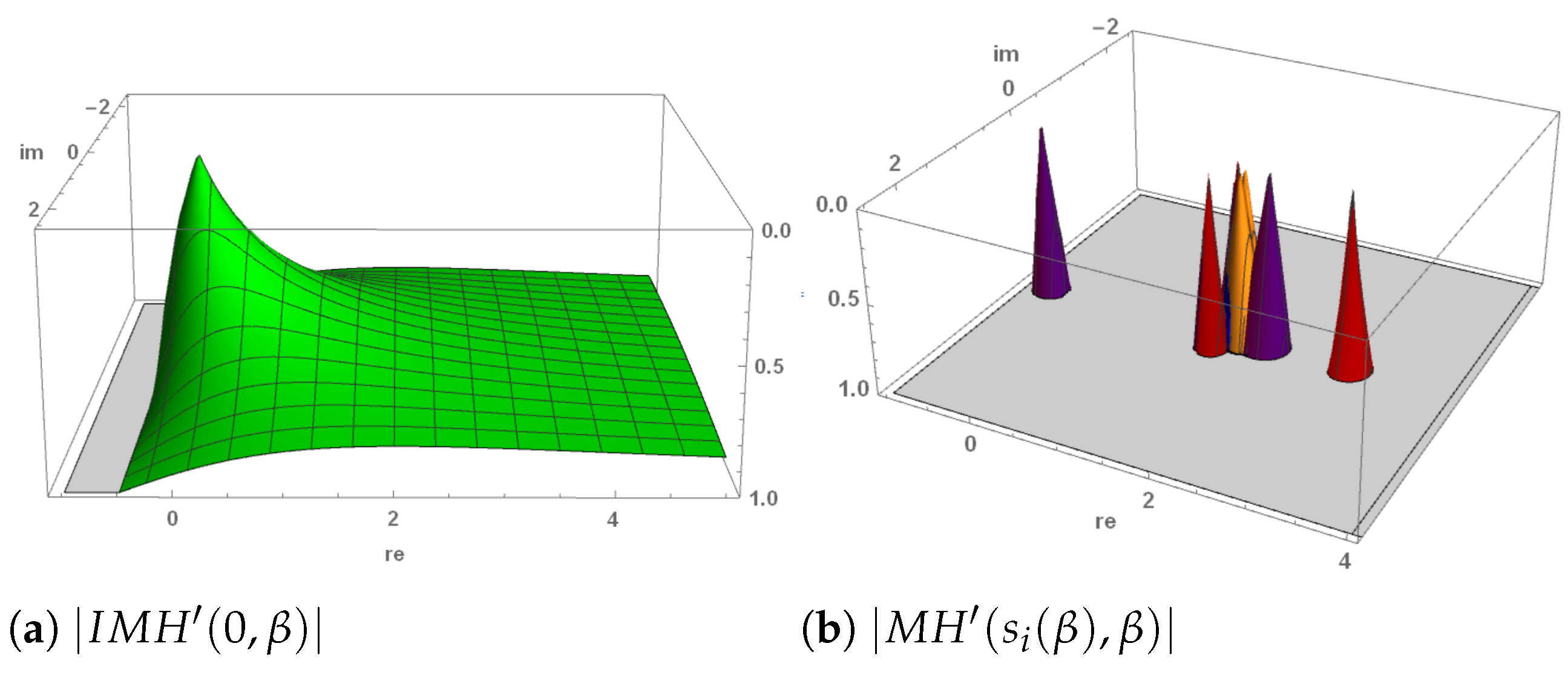
In Figure 1, the stability functions of the fixed points are presented. The code color is as follows: $s_1\left(\beta \right)$ is attracting for values of $\beta$ in orange regions, $s_2\left(\beta \right)$ is attracting where parameter $\beta$ belongs to red areas; blue color corresponds to values of $\beta$ where $s_3\left(\beta \right)$ is attracting and those where $s_4\left(\beta \right)$ is attracting are presented in purple color. In all cases, the vertices of the cones correspond to the values of $\beta$ where the related strange fixed point is superattracting.

So, it has been proven that the multiple root is always a superattracting fixed point, whereas the simple root can be repulsive (if $\Re \left(\beta \right)<-\frac{1}{2}$), parabolic for $\Re \left(\beta \right)=-\frac{1}{2}$ and attracting elsewhere. Moreover, there exist strange fixed points that can be attracting in small areas close to $\beta =0$.

Let us remark that, pretending to converge only to the multiple root, values of $\beta <-1$ will assure us the avoiding of basins of attraction of strange fixed points. However, if both simple and multiple root are searched, then the best values of the parameters to be chosen are $\beta =0$ (where the simple root is also superattracting, as the multiple one) or $\beta >4$, where all the strange fixed points $s_i\left(\beta \right)$ are repulsive.

3.2. Dynamical Planes

Each value of the parameter corresponds with a member of the class of iterative methods. When $\beta$ is fixed, the iterative process can be visualized in a dynamical plane. It is obtained by iterating the chosen element of the family under study, with each point of the complex plane as initial estimation. In this section, we have used a rectangular mesh of $800\times 800$, that is, we have considered a partition of the real and imaginary intervals in 800 subintervals. The nodes of this rectangular mesh are our starting points in the iterative processes. We represent in blue color those points whose orbit converges to infinity and in orange color the points converging to $z=0$, corresponding to the multiple root of $p\left(z\right)$ (with a tolerance of ${10}^{-3}$). Other colors (green, red, etc.) are used for those points whose orbit converges to one of the strange fixed points, marked as a white star in the figures if they are attracting or by a white circle if they are repulsive or parabolic. Moreover, a mesh point appears in black if it reaches the maximum number of 200 iterations without converging to any of the fixed points. The routines used appear in [19].

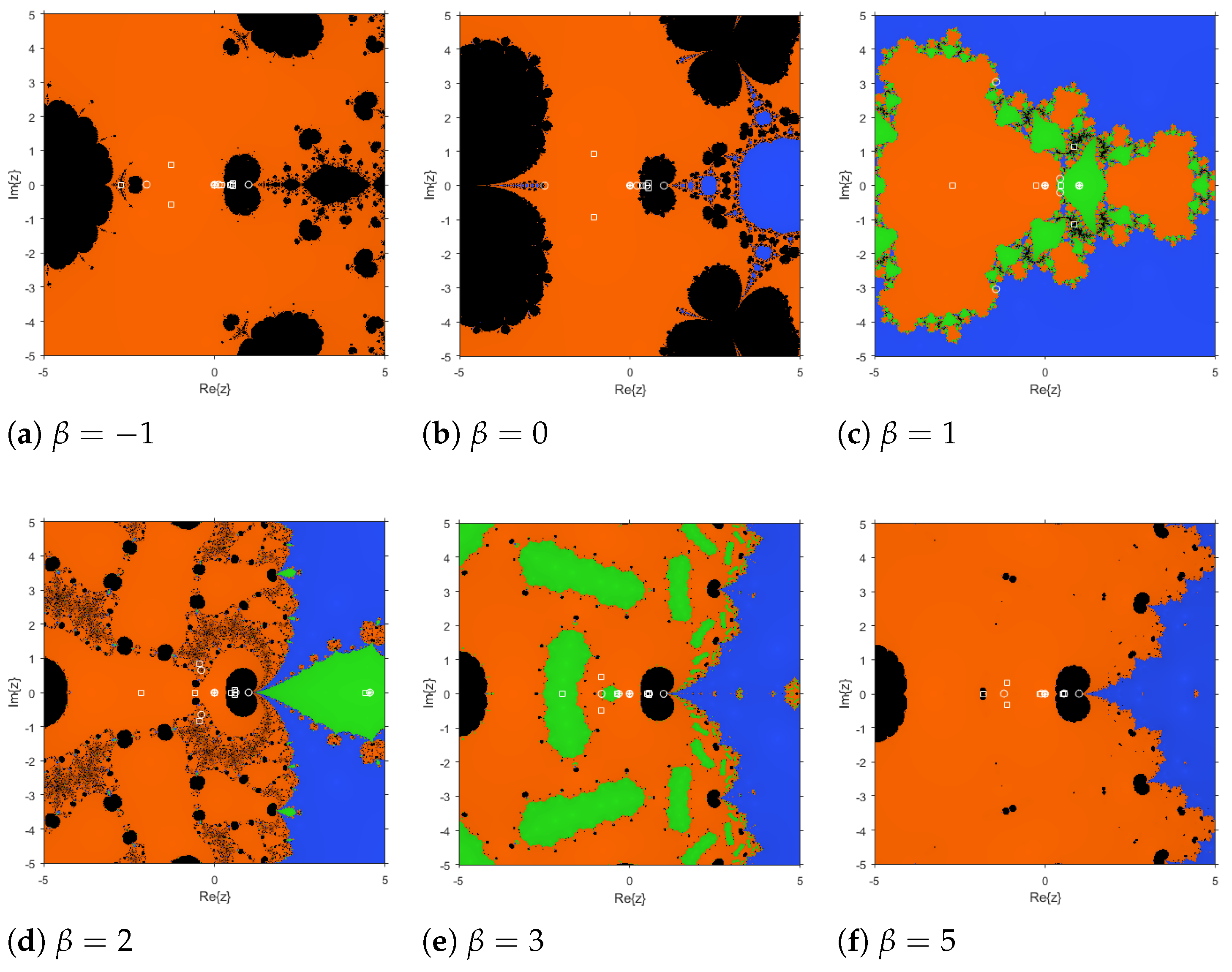
We plot the dynamical planes related to rational function $MH(z,\beta )$, for $\beta \in \{-1,0,1,2,3,5\}$. These planes can be visualized in Figure 2. In Figure 2a, orange area is the basin of attraction of $z=0$ (multiple root) and black points correspond to the attracting area of the parabolic fixed point $z=1$ and the basin of a periodic orbit of period 2; in cases of $\beta =0$ and $\beta =5$ (Figure 2b and f, respectively), the basin of attraction of the simple root ($z=\infty$) appears in blue, and in black the attracting area of the parabolic fixed point $z=1$; in Figure 2c–e, the basin of attraction of an strange fixed point appears in green color.

The information deduced from these planes confirm the theoretical results from Theorem 2 regarding the stability of the strange fixed points. The parabolic character of $z=1$ is the main drawback of the methods, as it is placed in the Julia set. However, in practice the rounding error will yield an initial estimation in the basin of $z=1$ to another the attracting fixed point.

4. Numerical Results

Here, we check the effectiveness of our newly proposed iterative methods. We employ some elements of our schemes: specifically scheme (18) for $\alpha =1$, $\alpha =\frac{1}{2}$, $\alpha =\frac{1}{10}$ and (19) for $\alpha =1$, $\alpha =\frac{1}{2}$, $\alpha =\frac{1}{4}$, denoted by $MHS1$, $MHS2$, $MHS3$, $MSHS1$, $MSHS2$ and $MSHS3$, respectively, to solve nonlinear equations mentioned in Examples 1–5.

We contrast our methods with existing schemes of same order: (3), (4), (5), (6) and (7), denoted by $CS$, $HS$, $OS$, $NS$ and $CN$, respectively. In

Table 1. Comparison of distinct iterative functions based on absolute residual errors and absolute difference between two consecutive iterations. * stands for convergence to undesired root.

Methods	I.G.	$\left|\mathit{f}\right({\mathit{x}}_{\mathit{\sigma }}\left)\right|$ $\parallel {\mathit{x}}_{\mathbf{\sigma }+\mathbf{1}}-{\mathit{x}}_{\mathbf{\sigma }}\parallel$	$\mathit{CS}$	$\mathit{HS}$	$\mathit{OS}$	$\mathit{ONS}$	$\mathit{CN}$	$\mathit{MHS}1$	$\mathit{MHS}2$	$\mathit{MHS}3$	$\mathit{MSHS}1$	$\mathit{MSHS}2$	$\mathit{MSHS}3$
Ex. (1)	$1.73$	$\left|f\right(x_6\left)\right|$	F	F	F	F	F	$1.3(-15)$	$3.0(-10)$	$2.0(-6)$	$7.7(-102)$	$2.0(-67)$	$2.2(-45)$
		$\parallel x_7-x_6\parallel$	F	F	F	F	F	$2.1(-7)$	$1.0(-4)$	$8.9(-3)$	$1.6(-50)$	$2.6(-33)$	$2.7(-22)$
Ex. (2)	$log5$	$\left|f\right(x_6\left)\right|$	F	F	F	F	F	$3.2(-97)$	$2.0(-228)$	$3.8(-179)$	$2.6(-122)$	$2.7(-404)$	$2.9(-924)$
		$\parallel x_7-x_6\parallel$	F	F	F	F	F	$3.5(-32)$	$6.5(-76)$	$1.7(-59)$	$1.5(-40)$	$1.5(-134)$	$7.4(-308)$
	$1.6$	$\left|f\right(x_6\left)\right|$	$Div$	$9.8(-2)$	$7.2(-464)$	$Div$	$Div$	$2.8(-97)$	$1.4(-228)$	$1.3(-179)$	$2.1(-122)$	$4.7(-404)$	$1.0(-926)$
		$\parallel x_7-x_6\parallel$	$Div$	$9.3(-1)$	$2.2(-154)$	$Div$	$Div$	$3.4(-32)$	$5.7(-76)$	$1.2(-59)$	$1.4(-40)$	$1.9(-134)$	$1.1(-308)$
Ex. (3)	$1.5$	$\left|f\right(x_6\left)\right|$	$2.9(-274)$ *	$2.2(-129)$	$7.6(-837)$	$Div$	$3.8(-582)$ *	$4.8(-593)$	$2.2(-652)$	$2.1(-294)$	$4.7(-1197)$	$8.4(-1217)$	$1.4(-1304)$
		$\parallel x_7-x_6\parallel$	$2.0(-55)$ *	$1.9(-26)$	$6.0(-168)$	$Div$	$5.2(-117)$ *	$3.4(-119)$	$4.7(-131)$	$1.8(-59)$	$8.6(-240)$	$6.1(-244)$	$1.7(-261)$
Ex. (4)	$4.4$	$\left|f\right(x_6\left)\right|$	$1.9(-142)$ *	$3.8(-375)$	$2.2(-694)$	$1.9(-142)$ *	$1.9(-142)$ *	$1.5(-497)$	$1.5(-613)$	$4.2(-462)$	$5.9(-705)$	$1.2(-828)$	$1.3(-1005)$
		$\parallel x_7-x_6\parallel$	$5.8(-48)$ *	$1.5(-125)$	$5.8(-232)$	$5.8(-48)$ *	$5.8(-48)$ *	$2.4(-166)$	$5.1(-205)$	$1.6(-154)$	$1.7(-235)$	$1.0(-276)$	$1.0(-335)$
	$1.7$	$\left|f\right(x_6\left)\right|$	$1.4(+7)$	$5.9(-331)$	$1.2(-646)$	$1.4(+7)$	$1.4(+7)$	$4.8(-403)$	$1.3(-566)$	$8.7(-427)$	$3.5(-669)$	$1.7(-865)$	$3.6(-885)$
		$\parallel x_7-x_6\parallel$	$1.5$	$8.1(-111)$	$4.7(-216)$	$1.5$	$1.5$	$7.5(-135)$	$2.3(-189)$	$9.2(-143)$	$1.5(-223)$	$5.3(-289)$	$1.5(-295)$
Ex. (5)		$\left|f\right(x_6\left)\right|$	$5.7(-14,352)$	$7.5(-21,328)$	$4.7(-34,103)$	$Div$	$5.3(-21,087)$	$3.1(-9344)$	$1.1(-13,965)$	$1.1(-19,577)$	$3.2(-23,126)$	$5.0(-40,450)$	$2.9(-38,495)$
		$\parallel x_7-x_6\parallel$	$1.0(-144)$	$1.8(-214)$	$3.2(-342)$	$Div$	$4.6(-212)$	$1.2(-94)$	$7.5(-141)$	$5.7(-197)$	$1.9(-232)$	$1.1(-405)$	$3.8(-386)$

,

Table 2. Contrast of distinct iterative methods based on number of iterations. * stands for convergence to undesired root.

Methods	I.G.	$\mathit{CS}$	$\mathit{HS}$	$\mathit{OS}$	$\mathit{ONS}$	$\mathit{CN}$	$\mathit{MHS}1$	$\mathit{MHS}2$	$\mathit{MHS}3$	$\mathit{MSHS}1$	$\mathit{MSHS}2$	$\mathit{MSHS}3$
Ex. (1)	$1.73$	F	F	F	F	F	9	10	11	7	8	8
Ex. (2)	$log5$	F	F	F	F	F	8	7	7	7	6	5
	$1.61$	$Div$	12	6	$Div$	$Div$	8	7	7	7	6	5
Ex. (3)	$1.5$	7 *	8	6	$Div$	6 *	6	6	7	6	6	6
Ex. (4)	$4.4$	7 *	6	6	7 *	7 *	6	6	6	6	6	5
	$1.7$	1280	6	6	1280	1280	6	6	6	6	6	6
Ex. (5)	$1.5$	6	6	5	$Div$	6	7	6	6	6	5	5

and

Table 3. Contrast of distinct iterative methods based on Computational order of convergence. * stands for convergence to undesired root.

Methods	I.G.	$\mathit{CS}$	$\mathit{HS}$	$\mathit{OS}$	$\mathit{ONS}$	$\mathit{CN}$	$\mathit{MHS}1$	$\mathit{MHS}2$	$\mathit{MHS}3$	$\mathit{MSHS}1$	$\mathit{MSHS}2$	$\mathit{MSHS}3$
Ex. (1)	$1.73$	$dne$	$dne$	$dne$	$dne$	$dne$	$3.000$	$3.000$	$3.000$	$3.000$	$3.000$	$3.000$
Ex. (2)	$log5$	$dne$	$dne$	$dne$	$dne$	$dne$	$3.000$	$3.000$	$3.000$	$2.999$	$3.002$	$2.993$
	$1.61$	$Div$	$3.000$	$3.000$	$dne$	$dne$	$3.000$	$3.000$	$3.000$	$2.999$	$3.002$	$3.002$
Ex. (3)	$1.5$	$3.000$ *	$3.000$	$3.000$	$dne$	$3.000$	$3.000$	$3.000$	$3.000$	$3.000$	$3.000$	$3.000$
Ex. (4)	$4.4$	$3.000$ *	$3.000$	$3.000$	$3.000$ *	$3.000$ *	$3.000$	$3.000$	$3.000$	$3.002$	$3.000$	$3.000$
	$1.7$	$3.000$	$3.000$	$3.000$	$3.000$	$3.000$	$3.000$	$3.000$	$3.000$	$2.998$	$3.000$	$3.000$
Ex. (5)		$3.000$	$3.000$	$3.000$	$3.000$	$dne$	$3.000$	$3.000$	$3.000$	$3.000$	$3.000$	$2.975$

, we display the values of absolute residual errors $\left|f\right(x_{\sigma +1}\left)\right|$, number of iterations in order to attain the desired accuracy, and the absolute errors $|x_{\sigma +1}-x_{\sigma }|$. Further, it is known that formula [20],

$$\rho \approx \frac{ln|(x_{\sigma +1}-\xi )/(x_{\sigma }-\xi )|}{ln|(x_{\sigma }-\xi )/(x_{\sigma -1}-\xi )|}.$$

displays the computational order of convergence, COC. In this estimation, we need to know the exact zero $\xi$ of the nonlinear function to be solved. But, there are several practical situations where the exact solution is not accessible. Therefore, Cordero and Torregrosa in [21], suggested the following estimation of the order of convergence, known as ACOC

$$\rho \approx \frac{ln|{\check{e}}_{\sigma +1}/{\check{e}}_{\sigma }|}{ln|{\check{e}}_{\sigma }/{\check{e}}_{\sigma -1}|},$$

(27)

where ${\check{e}}_{\sigma }=x_{\sigma }-x_{\sigma -1}$ and exact zero is not needed. In tables, *, $Div$ and F stand for converge to undesired root, case of divergence and case of failure, respectively. Moreover, $dne$ stands for does not exist.

During the current numerical experiments with programming language Mathematica (Version-9), all computations have been done with 1000 digits of mantissa, which minimize round-off errors. In tables, $(b_1\pm b_2)$ denotes $(b_1\times {10}^{\pm b_2})$. The configuration of the computer used is given below:

• Processor: Intel(R) Core(TM) i7-4790 CPU @ 3.60GHz
• RAM: 8:00GB
• System type: 64-bit-Operating System, x64-based processor.

Now, we explore the performance of our proposed methods, in comparison with known ones, on some chemical and engineering problems, that can be found in [22,23,24,25], among others.

Example 1.

Van der Waals equation of state (Case of failure):

$$\left(P+\frac{a_1{n}^2}{V^2}\right)(V-n{a}_2)=nRT,$$

describes the nature of a real gas between two gases $a_1$ and $a_2$, when we introduce the ideal gas equations. For calculating the volume V of the gases, we need the solution of preceding expression in terms of remaining constants,

$$P{V}^3-(n{a}_{2}P+nRT)V^2+{\alpha }_1{n}^{2}V-{\alpha }_1{\alpha }_2{n}^2=0.$$

By choosing the particular values of gases ${\alpha }_1$ and ${\alpha }_2$, we can easily obtain the values for n, P and T. Then, it yields

$$f_1\left(x\right)=x^3-5.22x^2+9.0825x-5.2675.$$

(28)

Function $f_1$ has 3 zeros, and among them $\xi =1.75$ is a multiple zero of multiplicity $m=2$ and $\xi =1.72$ is a simple zero. At the initial guess $1.73,$ which is quite close to our desired zero, all the known methods fail to work because the derivative turns zero at this initial point. But, our methods work even if the derivative is zero or close to zero. So, our methods are better than the existing one-point third-order methods. The results can be found in Table 1, Table 2 and Table 3.

Example 2.

Planck’s radiation problem (Case of failure and divergence):

Consider the Planck’s radiation equation that determines the spectral density of electromagnetic radiations released by a black-body at a given temperature, and at thermal equilibrium as

$$G\left(y\right)=\frac{8\pi ch{y}^{-5}}{e^{\frac{ch}{ykT}}-1},$$

where T, y, k, h, and c denotes the absolute temperature of the black-body, wavelength of radiation, Boltzmann constant, Plank’s constant, and speed of light in the medium (vacuum), respectively. To evaluate the wavelength y which results to the maximum energy density $G\left(y\right)$, set $G^{\prime }\left(y\right)=0$. Then, we obtain the following equation,

$$\frac{\left(\frac{ch}{ykT}\right)e^{\frac{ch}{ykT}}}{e^{\frac{ch}{ykT}}-1}=5.$$

Further, the nonlinear equation is reformulated by setting $x=\frac{ch}{ykT}$ as follows:

$$f_2\left(x\right)={\left(e^{-x}-1+\frac{x}{5}\right)}^3.$$

(29)

The exact zero of multiplicity $m=3$ is $\xi \approx 4.965114$, and with this solution one can easily find the wavelength y form the relation $x=\frac{ch}{ykT}$. Here, we can see that derivative is zero at $log5$. So, obviously the methods like $CS$, $HS$, $OS$, $ONS$ and $CN$ fail to work. With another choice of initial guess $1.61$, we found that the derivative is not zero but very close to zero. In this case, methods $CS$, $ONS$ and $CN$ diverge from the required root. On the other hand, our method is able to converge under these conditions. Methods $HS$ and $OS$ also converge to the required root but they are slower than our method $MSHS3$, because they are consuming 12 and 6 numbers of iterations respectively, as compared to our method $MSHS3$ that takes only 5 iterations. In this regards, please see the computational results in Table 1, Table 2 and Table 3.

Example 3.

Jumping and Oscillating problem, when we have infinite numbers of roots:

Here, we choose the following function for the computational results:

$$f_3\left(x\right)={\left(sinx\right)}^m,m=5$$

(30)

Function $f_3$ has infinite number of zeros but our desired zero is $\xi =0$ with multiplicity five. With the help this example, we aim to show that the convergence of an iterative method is not always guaranteed, even though we choose a nearest initial point. For example, methods $CS$ and $CN$ with $x_0=1.5$ are unsuitable because of numerical instability, which occurs due to large value of the correction factor and it converges to $442\pi$ and $5\pi$, respectively, far away from the required zero. On the other hand, Osada’s method $ONS$ diverges for the starting point $x_0=1.5$. Therefore, care must be taken to ensure that the root obtained is the desired one. But, there is no such problems with our methods. The details of the computational results can be found in Table 1, Table 2 and Table 3.

Example 4.

Convergence to the undesired root problem:

So, we consider an academical problem, which is given as follows:

$$f_4\left(x\right)={\left(e^{-x}+sinx\right)}^3.$$

(31)

Expression (31) has an infinite number of roots with multiplicity three, being our desired root $\xi \approx 3.183063$. It can be seen that $CS$, $ONS$, and $CN$ converge to undesired zero $6.281314$, after finite number of iteration when $x_0=4.4$. On the other hand, with initial guess $1.7$ methods $CS$, $ONS$, and $CN$ consume 1280 number of iterations as compared to 6. The computational outcomes are given in Table 1, Table 2 and Table 3.

Example 5.

Finally, we consider an academical problem with higher order of multiplicity $m=100$, which is defined by

$$f_5\left(x\right)={\left({(x-1)}^3-1\right)}^{100}.$$

(32)

Expression (32) has a zero $x=2$ of multiplicity 100. We show the computational results based on the function $f_5$ in Table 1, Table 2 and Table 3. From the numerical results, we conclude that our methods $MSH2$ and $MSH3$ need the same number of iterations in order to reach the desired accuracy, but they have smaller residual errors and smaller differences between two consecutive iterations as compared to other existing methods.

5. Concluding Remarks

In this paper, we have suggested a new family of point-to-point third-order iterative methods that works for multiple roots ($m\ge 1$), where the multiplicity of the root is known in advance; moreover, they converge to the required root even in the case of failure or divergence, or oscillation, retaining the third-order of convergence. In addition to this, one of the most popular third-order methods namely Chebyshev, Halley and super-Halley all are the special cases of our scheme, when $m=1$. Our scheme is based on a geometrical derivation rather than derivation on some interpolations or weight function or analytic approaches, etc. Complex dynamics has been used to check the stability of the class of iterative methods. Finally, based on the numerical results, we concluded that our methods not only perform better in the case of failure, divergence and oscillations but also in the convergence cases. In the future, we will work on the multi-point variants of our family (16) by estimating the second-order derivatives.