Nonsmooth Optimization-Based Hyperparameter-Free Neural Networks for Large-Scale Regression

Abstract

In this paper, a new nonsmooth optimization-based algorithm for solving large-scale regression problems is introduced. The regression problem is modeled as fully-connected feedforward neural networks with one hidden layer, piecewise linear activation, and the $L_1$-loss functions. A modified version of the limited memory bundle method is applied to minimize this nonsmooth objective. In addition, a novel constructive approach for automated determination of the proper number of hidden nodes is developed. Finally, large real-world data sets are used to evaluate the proposed algorithm and to compare it with some state-of-the-art neural network algorithms for regression. The results demonstrate the superiority of the proposed algorithm as a predictive tool in most data sets used in numerical experiments.

1. Introduction

Regression models and methods are extensively utilized for prediction and approximation in various real-world scenarios. When data involve complex relationships between the response and explanatory variables, regression methods designed using neural networks (NNs) have emerged as powerful alternatives to traditional regression methods [1]. Hence, we focus on NNs for regression (NNR): we introduce a new approach for modeling and solving regression problems using fully-connected feedforward NNs with the rectified linear unit (ReLU) activation function, the $L_1$-loss function, and the $L_1$-regularization. We call this problem the ReLU-NNR problem, and the method for solving it is the limited memory bundle NNR (LMBNNR) algorithm.

The ReLU-NNR problem is nonconvex and nonsmooth. Note that ReLU itself is nonsmooth. Thus, even if we used a smooth loss function and regularization, the underlying optimization problem would still be nonsmooth. Conventional global optimization methods, including those based on global random search, become time-consuming as this problem contains a large number of variables. In addition, the authors in [2] showed that it is impossible to give any guarantee that the global minimizer is found by a general global (quasi-)random search algorithm with reasonable accuracy when the dimension is large. On the other hand, local search methods are sensitive to the choice of starting points and, in general, end up at the closest local solutions, which may be significantly different from the global ones. To address the nonconvexity of the ReLU-NNR problem, we propose a constructive approach. More specifically, we construct initial weights by using the solution from the previous iteration. Such an approach allows us to find either global or deep local minimizers for the ReLU-NNR problem. To solve the underlying nonsmooth optimization problems, we apply a slightly modified version of the limited memory bundle method (LMBM) developed by Karmitsa (née Haarala) [3,4]. We use this method since it is one of the few algorithms capable of handling large dimensions, nonconvexity, and nonsmoothness all at once. In addition, the LMBM has already proven itself in solving machine learning problems such as clustering [5], cardinality and clusterwise linear regression [6,7], and missing value imputation  [8].

We consider NNs with only one hidden layer but the number of hidden nodes is determined automatically using a novel constructive approach and an automated stopping procedure (ASP). More precisely, the number of nodes is determined incrementally by starting from one node. ASP bases the intelligent selection of initial weights on the iteratively self-updated regularization parameter. It is applied at each iteration of the constructive algorithm to stop training if there is no further improvement in the model. Thus, there are no tuneable hyperparameters in LMBNNR.

To summarize, the LMBNNR algorithm has some remarkable features, including:

• It takes full advantage of nonsmooth models and nonsmooth optimization in solving NNR problems (no need for smoothing etc.);
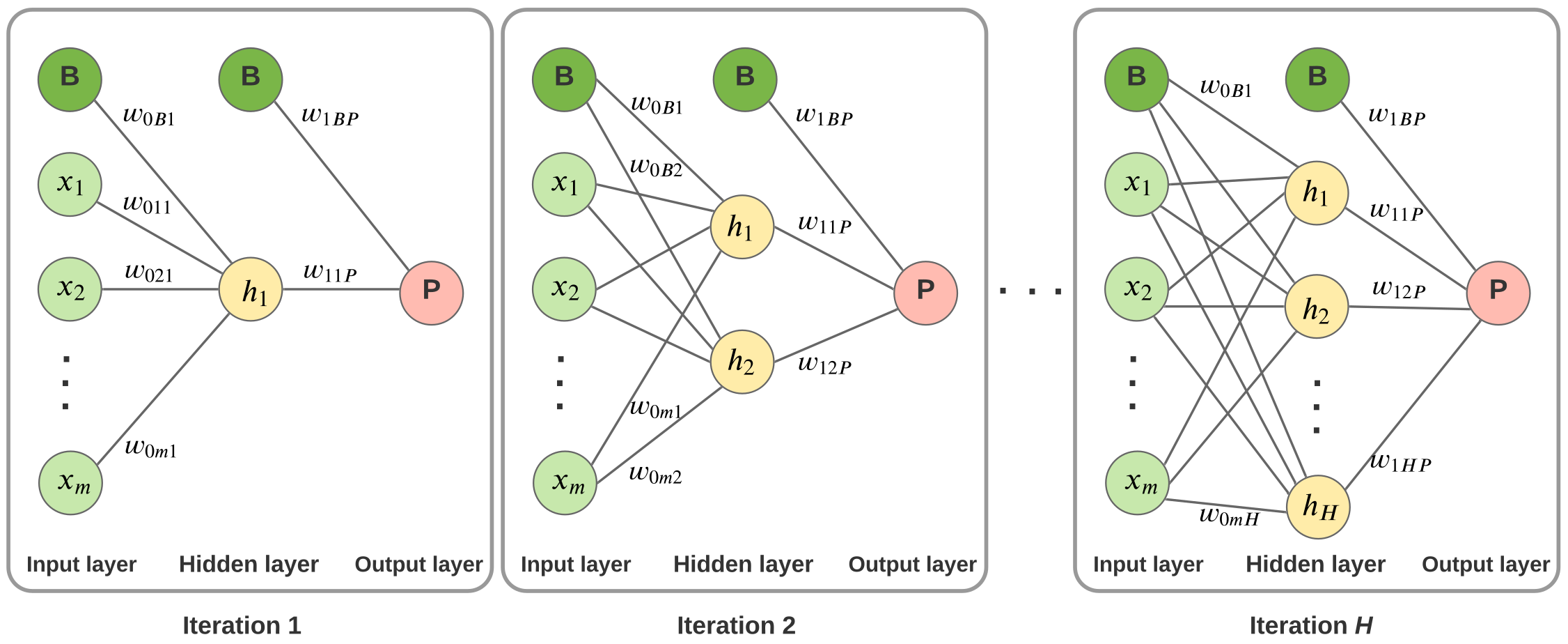
• It is hyperparameter-free due to the automated determination of the proper number of nodes;
• It is applicable to large-scale regression problems;
• It is an efficient and accurate predictive tool.

The structure of the paper is as follows. An overview of the related work is given in Section 2, while Section 3 provides the theoretical background on nonsmooth optimization and NNR. The problem statement—the ReLU-NNR problem—is given in Section 4, and in Section 5, the LMBNNR algorithm together with ASP is introduced. In Section 6, we present the performance of the LMBNNR algorithm and compare it with some state-of-the-art NNR algorithms. Section 7 concludes the paper.

2. Related Work

Optimization is at the core of machine learning. Although it is a well-known fact that many machine learning problems lead to solving nonsmooth optimization problems (e.g., hinge-loss, lasso, and ReLU), nonsmooth optimization methods are scarcely used in the machine learning society. The common practice is to minimize nonsmooth functions by ignoring the nonsmoothness and employing a popular and simple smooth solver (like the Newton method, e.g., [9]) or by applying some smoothing techniques (see, e.g., [10,11]). However, there are some successful exceptions. For example, abs-linear forms of prediction tasks are solved using a successive piecewise linearization method in [12,13], a primal-dual prox method for problems in which both the loss function and the regularizer are nonsmooth is developed in [14], various nonsmooth optimization methods are applied to solve clustering, classification, and regression problems in [5,6,15,16,17], and finally, nonsmooth optimization approaches are combined with support vector machines in [18,19,20].

NNs are among the most popular and powerful machine learning techniques. There are two main properties in any NNs: an activation function and an error (loss) function. The simplest activation function is linear, and NNs with this function can be easily trained. Nevertheless, they cannot learn complex mapping functions, resulting in a poor outcome in the testing phase. On the other hand, smooth nonlinear activation functions, like the sigmoid and the hyperbolic tangent activation functions, may lead to highly complex nonconvex loss functions and require numerous training iterations as well as many hidden nodes [21].

In [22], it is theoretically discussed that NNs with nonsmooth activation functions demonstrate high performance. Among these functions, the piecewise linear ReLU has lately become the default activation function for many types of NNs. This function is nonsmooth, but it has a simple mathematical form of $f\left(x\right)=max\{0,x\}.$ ReLU provides more sensitivity to the summed activation of the node compared with traditional smooth sigmoid and hyperbolic tangent functions, and it avoids easy saturation. Due to the computational advantages of its simple structure and, thus, strong training ability, ReLU is preferable for training complex relationships in NNs. In practice, instead of minimizing the resultant nonsmooth loss function directly, it is often replaced with a smoothed surrogate loss function (see, e.g., [11]). However, algorithms based on smoothing techniques involve the choice of smoothing parameters. The number of such parameters becomes large in large data sets, and their choice becomes problematic, which affects the accuracy of algorithms.

The stochastic (sub)gradient descent method (SGD) is another commonly used method to minimize the loss function in NNs algorithms. Although this method has been used intuitively to solve machine learning problems with nonsmooth activation and loss functions for years, its convergence for such functions has been proved only very recently [23]. SGD is efficient since it does not depend on the size of the data, but it is not accurate as an optimization method and may require a large number of function and subgradient evaluations. Moreover, SGD may easily diverge if the learning rate (step size) is too large. These drawbacks are due to the fact that SGD is based on the subgradient method for convex problems, while NNs problems are highly nonconvex. For more discussions on NNs, we refer to [24].

The most commonly used NNR algorithms are the feedforward backpropagation network (FFBPN) [25,26,27,28] and the radial-basis network (RBN) [29,30,31]. FFBPN and most of its variants converge to only locally optimal solutions [26,27], and they only work under the precondition that all the functions involved in NNR are differentiable. RBN and its modifications can be trained without local minima issues [32], but they involve a heuristic procedure to select parameters and hyperparameters.

The choice of the hyperparameters in NNs is a challenging problem. These parameters define the structure of NNs, and their optimal choice leads to an accurate model. Generally, the hyperparameters can be determined either by an algorithm or manually by the user. Tuning the hyperparameters manually is a tedious and time-consuming process, and thus, several algorithms with varying levels of automaticity have been proposed for this purpose (see, e.g., [33,34,35,36,37,38]). Nevertheless, there is no guarantee that in these algorithms the selected number of hidden units (usually the number of nodes) is optimal, and the question of a good hyperparameter tuning procedure remains open. Therefore, it is imperative to develop algorithms that can minimize nonsmooth loss functions as they are (i.e., without smoothing) and automate the calibration of the hyperparameters.

3. Theoretical Background and Notations

In this section, we provide some theoretical background and notations that are used throughout the paper.

3.1. Nonsmooth Optimization

Nonsmooth optimization refers to the problem of minimizing (or maximizing) functions that are not continuously differentiable [39]. We denote the d-dimensional Euclidean space by ${\mathbb{R}}^d$ and the inner product by $x^{\top }y={\sum }_{i=1}^d{x}_i{y}_i$, where $x,y\in {\mathbb{R}}^d$. The associated $L_2$ and $L_1$-norms are ${\parallel x\parallel }_2={\left(x^{\top }x\right)}^{1/2}$ and ${\parallel x\parallel }_1={\sum }_{i=1}^d\left|x_i\right|$, respectively.

A function $f:{\mathbb{R}}^d\to \mathbb{R}$ is called locally Lipschitz continuous on ${\mathbb{R}}^d$ if for any bounded subset $X\subset {\mathbb{R}}^d$ there exists $L>0$ such that

$$\begin{array}{c}\hfill |f\left(x\right)-f\left(y\right)|\le {L\parallel x-y\parallel }_2\mathrm{for}\mathrm{all}x,y\in X.\end{array}$$

The Clarke subdifferential $\partial f\left(x\right)$ of a locally Lipschitz continuous function $f:{\mathbb{R}}^d\to \mathbb{R}$ at a point $x\in {\mathbb{R}}^d$ is given by [39,40]

$$\partial f\left(x\right)=conv\left\{\underset{i\to \infty }{lim}\nabla f\left(x^i\right)\mid x^i\to x\mathrm{and}\nabla f\left(x^i\right)\mathrm{exists}\right\},$$

where “conv” denotes the convex hull of a set. A vector $\xi \in \partial f\left(x\right)$ is called a subgradient. The point $x^{*}\in {\mathbb{R}}^d$ is stationary, if $0\in \partial f\left(x^{*}\right)$. Note that stationarity is a necessary condition for local optimality [39].

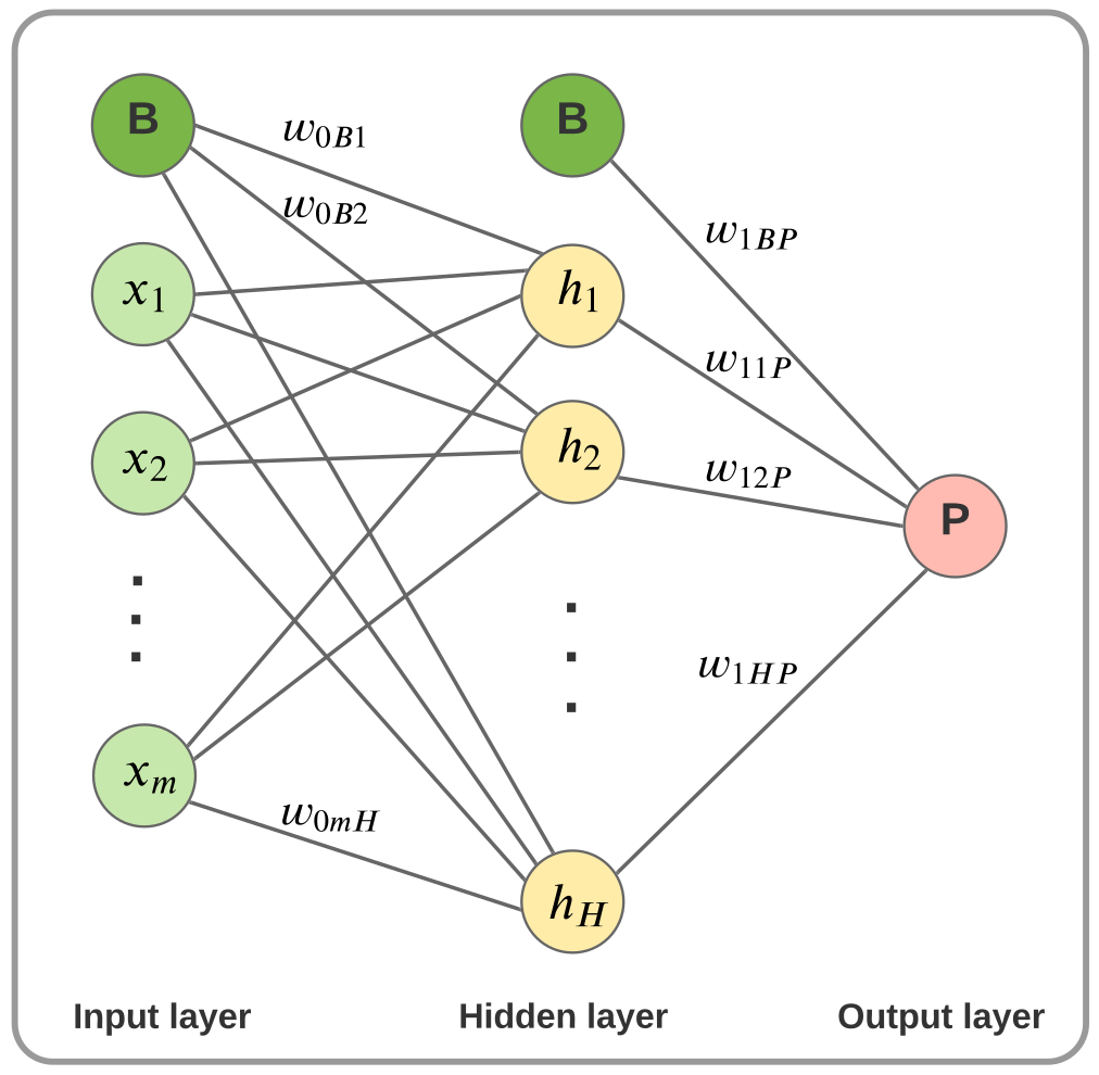
3.2. Neural Networks for Regression

Let A be a given data set with n samples: $A=\{(x^i,y_i)\in {\mathbb{R}}^m\times \mathbb{R}\mid i=1,\dots ,n\}$, where $x^i\in {\mathbb{R}}^m$ are the values of m input features and $y_i\in \mathbb{R}$ are their outputs. In regression analysis, the aim is to find a function $\phi :{\mathbb{R}}^m\to \mathbb{R}$ such that $\phi \left(x^i\right)$ is a “good approximation” of $y_i$. In other words, the following regression error is minimized:

$$\sum _{i=1}^n{|\phi \left(x^i\right)-y_i|}^p,p>0.$$

(1)

Applying NNs to the regression problem can lead to significantly higher predictive power compared with traditional regression. In addition, it can model more complex scenarios just by increasing the number of nodes. This concept is proved in the universal approximation theorem, which states that a single hidden layer feedforward network of sufficient complexity is able to approximate any given regression function on a compact set to an arbitrary degree [41].

In practice, NNs take several input features and, as a part of the learning process, multiply them by their weights and run them through an activation function and a loss function, which closely resemble the regression error (1). The loss function is used to estimate the error in the current model so that the weights can be updated to reduce this error on the next evaluation. The most commonly used loss function for NNR problems is the mean squared error (MSE or $L_2$-norm). However, there are at least two valid reasons to choose the mean absolute error (MAE or $L_1$-norm) over the $L_2$-norm: first, the $L_1$-norm makes the loss function with the ReLU activation function simpler, and second, the regression models with the $L_1$-norm are more robust to outliers (see, e.g., [42]). Once the is trained, the optimal weights for the model (regression coefficients) are found to fit the data.

4. Nonsmooth Optimization Model of ReLU-NNR

In this section, we formulate the nonsmooth optimization model for the RELU-NNR problem, but first, we give some notations. Let us denote the number of hidden nodes in NNs by H and let w be the weight connection vector and $w_s$ be its element in the index place s, where s is the index triplet $s=abc$ (see Figure 1). Then $w_{abc}$ states the weight that connects a-th layer’s b-th node to $(a+1)$-th layer’s c-th node. In addition, denote by P an output index value for the weights connecting the hidden layer’s nodes to the output node of the NN. In contrast to the hidden nodes, no activation function is applied to the output node. Finally, let B denote the middle index value for the weights connecting a layer’s bias term to a node in the next layer. The bias terms with this index can be thought of as the last node in each layer. The weight connection vector w for m input features and H hidden nodes has $H(m+2)+1$ components. For the sake of clarity, we organize $w=w^H$ in an “increasing order” as

$$\begin{array}{cc}\hfill w^H=& (w_{011},w_{012},\dots ,w_{01H},w_{021},w_{022},\dots ,w_{02H},\dots ,\hfill \\ \hfill & w_{0m1},w_{0m2},\dots ,w_{0mH},w_{0B1},w_{0B2},\dots ,w_{0BH},\hfill \\ \hfill & w_{11P},w_{12P},\dots ,w_{1HP},w_{1BP}{)}^{\top }.\hfill \end{array}$$

We define the following

$$\begin{array}{cc}\hfill s_{ij}& =w_{0Bj}+\sum _{k=1}^m{w}_{0kj}{x}_k^i,i=1,\cdots ,n,j=1,\cdots ,H,\hfill \\ \hfill t_i& =w_{1BP}+\sum _{j=1}^H{w}_{1jP}max\{0,s_{ij}\},i=1,\cdots ,n,\hfill \end{array}$$

where $x_k^i$ denotes the k-th coordinate of the i-th sample. The loss function using the $L_1$-norm (cf. regression error (1) with $p=1$) is

$$F_H\left(w\right)=\sum _{i=1}^n|t_i-y_i|.$$

(2)

To avoid overfitting in the learning process, we add an extra element to the loss function $F_H$. In most cases, $L_1$-regularization is preferable as it reduces the weight values of less important input features. In addition, it is robust and insensitive to outliers. Thus, we rewrite (2) as

$$f_H\left(w\right)=F_H\left(w\right)+{\rho }_H{\parallel w\parallel }_1,$$

where ${\rho }_H>0$ is an iteratively self-updated regularization parameter (to be described later). Furthermore, the nonsmooth, nonconvex optimization formulation for ReLU-NNR can be expressed as

$$\begin{array}{c}\hfill \left\{\begin{array}{cc}\mathrm{minimize}\hfill & f_H\left(w\right)\hfill \\ \mathrm{subject}\mathrm{to}\hfill & w\in {\mathbb{R}}^{H(m+2)+1}.\hfill \end{array}\right.\end{array}$$

(3)

5. LMBNNR Algorithm

To solve the ReLU-NNR problem (3), we now introduce the LMBNNR algorithm. In addition, we recall the LMBM in the form used here and briefly discuss its convergence. A more detailed description of the algorithm can be found in the technical report [43].

The LMBNNR algorithm computes hidden nodes incrementally and uses ASP to detect the proper number of these nodes. More precisely, it starts with one node in the hidden layer and adds a new node to that layer at each iteration of the algorithm. It is worth noting that each time a node is added, $m+2$ new connection weights appear. Starting from the initial weight $w^1\in {\mathbb{R}}^{m+3},$ the LMBNNR algorithm (Algorithm 1) applies the LMBM (Algorithm 2) to solve the underlying ReLU-NNR problem. The solution is employed to generate initial weights for the next iteration. This procedure is repeated until ASP is activated or the maximum number of hidden nodes $H_{max}$ is reached. ASP is designed based on the value of the objective function; if the value of the objective is not improved in three subsequent iterations, then the LMBNNR algorithm is stopped. Note that the initialization of weights and the regularization parameter (described below) are determined in such a way that we have $f_H\ge f_{H+1}$ for all $H=1,\cdots ,H_{max}$ and $f_H$ is an optimal value of (3) with H nodes.

We select the initial weights $w^1$ as

$$w^1={\left(\frac{1}{m},\frac{1}{m},\cdots ,\frac{1}{m},0,1,0\right)}^{\top }\in {\mathbb{R}}^{m+3}.$$

Here, the first m components are the weights from the nodes of the input layer to the node of the hidden layer. The weights from the bias terms $w_{1BP}$ and $w_{0B1}$ are set to zero, and the weight $w_{11P}$ from the hidden layer to the output is set to one. Figure 2 illustrates the weights in different iterations and the progress of the LMBNNR algorithm.

At subsequent iterations $H=2,\cdots ,H_{\mathrm{final}}$ (i.e., when we add a new node to the hidden layer, here $H_{\mathrm{final}}$ is the final number of hidden nodes), we initialize the weights $w^H$ as follows: let ${\overline{w}}^{H-1}$ be the solution to the $(H-1)$-th ReLU-NNR problem. First, we set weights for all but the last two hidden nodes in the output layer as

$$\begin{array}{cc}\hfill & w_{1jP}^H={\overline{w}}_{1jP}^{H-1}\mathrm{for}\mathrm{all}j=1,\cdots ,H-2,\hfill \\ \hfill & w_{1BP}^H={\overline{w}}_{1BP}^{H-1}\hfill \end{array}$$

(4)

and the weights from the input layer to all but the last two hidden nodes as

$$\begin{array}{cc}\hfill & w_{0ij}^H={\overline{w}}_{0ij}^{H-1}\mathrm{for}\mathrm{all}i=1,\cdots ,m,j=1,\cdots ,H-2,\hfill \\ \hfill & w_{0Bj}^H={\overline{w}}_{0Bj}^{H-1}\mathrm{for}\mathrm{all}j=1,\cdots ,H-2.\hfill \end{array}$$

(5)

Note that in the case of $H=2$, we set $w_{1BP}^2={\overline{w}}_{1BP}^1$. Otherwise, we skip this step as there are only two nodes in the hidden layer. Then we take the most recent weights obtained at the previous iteration and split these weights to get the initial weights connecting the input layer and the last two hidden nodes of the current iteration, that is,

$$\begin{array}{cc}\hfill & w_{0iH}^H=w_{0i(H-1)}^H=\frac{1}{2}{\overline{w}}_{0i(H-1)}^{H-1}\mathrm{for}\mathrm{all}i=1,\cdots ,m,\hfill \\ \hfill & w_{0BH}^H=w_{0B(H-1)}^H=\frac{1}{2}{\overline{w}}_{0B(H-1)}^{H-1}.\hfill \end{array}$$

(6)

Weights from the last two hidden nodes to the output are

$$\begin{array}{c}\hfill w_{1HP}^H=w_{1(H-1)P}^H={\overline{w}}_{1(H-1)P}^{H-1}.\end{array}$$

(7)

To update the regularization parameter ${\rho }_H$, we use the value of the objective at the previous iteration and the weight connecting the newest node of the hidden layer to the output as follows:

$$\begin{array}{c}\hfill {\rho }_H={\rho }_{H-1}·\frac{f_{H-1}}{f_{H-1}+\left|w_{1HP}^H\right|},\mathrm{with}{\rho }_1=1.0.\end{array}$$

(8)

Remark 1.

With the used initialization of weights $w^H$ and the regularization parameter ${\rho }_H$ we always have $f_H\ge f_{H+1}$ for $H=1,\cdots ,H_{\mathrm{final}}.$ ASP is activated if the value of the objective is no longer improving. In other words, when adding more nodes to the hidden layer does not give us a better model after optimization of the weights.

Now we are ready to give the LMBNNR algorithm.

Algorithm 1: LMBNNR

Remark 2.

There are no tuneable hyperparameters in LMBNNR. Hence, there is no need for a validation set. It is sufficient to choose the maximum number of hidden nodes $H_{max}$ big enough (see Section 6 for suitable values).

Next, we describe the LMBM with slight modifications to its original version for solving the underlying ReLU-NNR problems in the LMBNNR algorithm. This method is called at every iteration of LMBNNR. For more details of the LMBM, we refer to [3,4].

Remark 3.

We use a nonmonotone line search [4,44] to find step sizes $t_L^k$ and $t_R^k$ when Algorithm 2 is combined with Algorithm 1. In addition, as in [9], we use a relatively low maximum number of iterations, $k_{max}$, to avoid overfitting.

Remark 4.

The search direction in Algorithm 2 is computed using the L-BFGS update after a serious step and the L-SR1 update after a null step. The updating formulae are similar to those in the classical limited memory variable metric methods for smooth optimization [45]. Nevertheless, the correction vectors $u_k$ and $s_k$ are obtained using subgradients instead of gradients and the auxiliary point instead of the new iteration point.

Remark 5.

The classical linearization error may be negative in the case of a nonconvex objective function. Therefore, a subgradient locality measure ${\beta }_k$, which is a generalization of the linearization error for nonconvex functions (see, e.g., [46]), is used in Algorithm 2.

Algorithm 2: LMBM for ReLU-NNR problems

We now recall the convergence properties of the LMBM in the case of ReLU-NNR problems. Since the objective function $f_H:{\mathbb{R}}^{H(m+2)+1}\to \mathbb{R}$ is locally Lipschitz continuous and upper semi-smooth (see e.g., [47]), and the level set $\{w^H\in {\mathbb{R}}^{H(m+2)+1}\mid f_H\left(w^H\right)\le f_H\left(w_1^H\right)\}$ is bounded for every starting weight $w_1^H\in {\mathbb{R}}^{H(m+2)+1}$, all the assumptions needed for the global convergence of the original LMBM are satisfied. Therefore, the theorems on the convergence of the LMBM proved in [3,4] can be modified for the ReLU-NNR problems as follows.

Theorem 1.

If the LMBM terminates after a finite number of iterations, say at iteration k, then the weight $w_k^H$ is a stationary point of the  ReLU-NNR problem (3).

Theorem 2.

Every accumulation point ${\overline{w}}^H$ of the sequence $\left\{w_k^H\right\}$ generated by the  LMBM is a stationary point of the  ReLU-NNR problem (3).

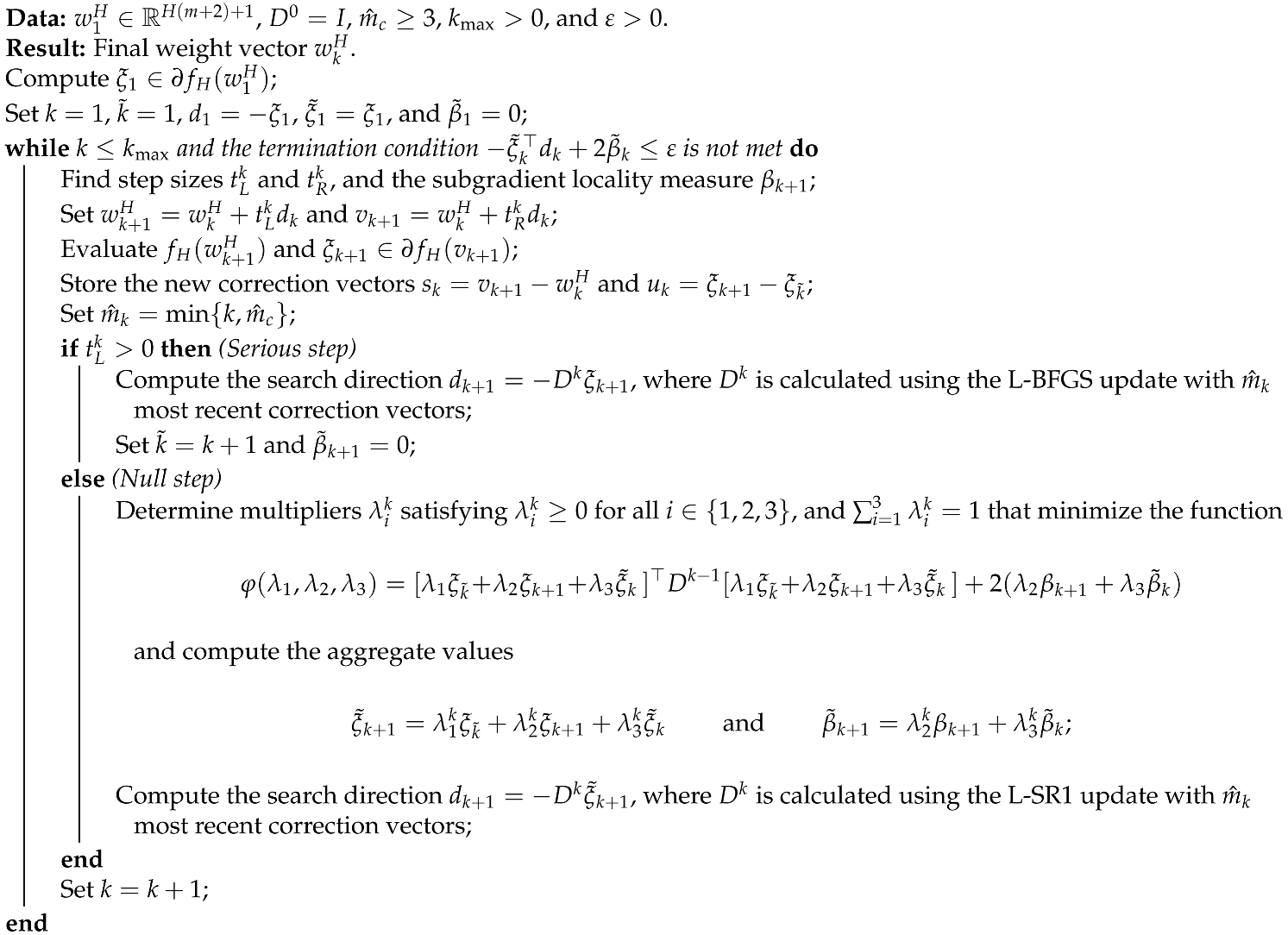
6. Numerical Experiments

Using some real-world data sets and performance measures, we evaluate the performance of the proposed LMBNNR algorithm. In addition, we compare it with three different widely used NNR algorithms whose implementations are freely available. That is, the backpropagation NNR (BPN) algorithm utilizing TensorFlow (https://www.tensorflow.org/(accessed on 10 September 2023)), Extreme Learning Machine (ELM) [48], and Monotone Multi-Layer Perceptron Neural Networks (MONMLP) [49].

6.1. Data Sets and Performance Measures

A brief description of data sets is given in

Table 1. Brief description of data sets.

Data Set	No. of Samples	No. of Features	Reference
Combined cycle power plant	9568	5	[50,51]
Airfoil self-noise	1503	6	[52]
Concrete compressive strength	1030	9	[53]
Physicochemical properties
of protein tertiary structure	45,730	10	[52]
Boston housing data	506	14	[54]
SGEMM GPU kernel performance 1	241,600	15	[55,56]
Online news popularity	39,644	59	[57]
Residential building data set 1	372	108	[58]
BlogFeedback 2	52,397	281	[59]
ISOLET	7797	618	[52]
CIFAR-10	60,000	3073	[60]
Greenhouse gas observing network	2921	5232	[61]

¹ Used with the first output feature. ² Only the training data set.

and the references therein. The data sets are divided randomly into training (80%) and test (20%) sets. To get comparable results, we use the same training and test sets for all the methods. We apply the following performance measures: root mean square error (RMSE), mean absolute error (MAE), coefficient of determination ($R^2$), and Pearson’s correlation coefficient (r) (see the Supplementary Material for more details).

6.2. Implementation of Algorithms

The proposed LMBNNR algorithm was implemented in Fortran 2003, and the computational experiments were carried out on an iMac (macOS Big Sur 11.6) with a 4.0 GHz Intel(R) Core(TM) i7 machine and 16 GB of RAM. The source code is available at http://napsu.karmitsa.fi/lmbnnr (accessed on 10 September 2023). There are no tuneable parameters in the LMBNNR algorithm.

The BPN algorithm is implemented using TensorFlow in Google Colab. We use the ReLU activation for the hidden layer, the linear activation for the output layer, and the MSE loss function. We use MSE since it usually worked better than MAE in our preliminary experiments with the BPN algorithm. This is probably due to the smoothness of MSE. Naturally, with the proposed LMBNNR algorithm, we do not have difficulties with the nonsmoothness as it applies the nonsmooth optimization solver LMBM. In the BPN algorithm, the Keras optimizer SGD with the default parameters and the following three different combinations of batch size (the number of samples that will be propagated through the network) and number of epochs (the number of complete passes through the training data) are used:

• Mini-Batch Gradient Descent (MBGD): batch size $=32$ and number of epochs $=1.$ These are the default values for the BPN algorithm;
• Batch Gradient Descent (BGD): batch size = size of the training data and number of epochs $=1$. These choices mimic the proposed LMBNNR algorithm;
• Stochastic Gradient Descent (SGD): batch size $=1$ and number of epochs $=100$ for data sets with less than 100,000 samples and number of epochs $=10$ for larger data. We reduce the number of epochs in the latter case due to very long computational times and the fact that the larger number of epochs often leads to NaN loss function values. SGD aims to be as a stochastic version of the BPN algorithm as possible.

The algorithms ELM and MONMLP are implemented in R using the packages “elmNNRcpp” (ELM is available at https://CRAN.R-project.org/package=elmNNRcpp (accessed on 10 September 2023)) and “monmlp” (MONMLP is available at https://CRAN.R-project.org/package=monmlp (accessed on 10 September 2023)). The parameters are the default values provided in the given references, but the number of hidden layers with MONMLP was set to one. The tests with ELM and MONMLP were run on Windows, 2.6 GHz Intel(R) Core(TM) i7-9750H. We run ELM, MONMLP, and the BPN algorithms with the number of hidden nodes set to 2, 5, 10, 50, 100, 200, 500, and 5000. Moreover, since SGD is used as an optimizer in the BPN algorithms as a stochastic method, we run the BPN algorithms ten times for all problems and report the average. Note that LMBNNR needs to be applied to solve the ReLU-NNR problem only once for each data set.

Remark 6.

At every iteration of the LMBNNR algorithm, we solve an optimization problem with the dimension $H(m+2)+1$, where H is the number of hidden nodes and m is the number of features in training samples. The convergence rate of the LMBM, employed as an underlying solver in the proposed LMBNNR algorithm, has not been studied extensively, but, as a bundle method, it is at most linear (see, e.g., [62]), while the search direction can be computed within $O\left(m\right)$ operations [3]. For comparison purposes, we mention that the time complexity of a BPN algorithm is typically $O\left(n\right)$, where n is the number of training samples. A more specific analysis of the time complexity of LMBNNR remains a subject for future research.

6.3. Results and Discussion

The results of our experiments are given in

Table 2. Results with relatively small numbers of features.

	LMBNNR		MBGD		BGD		SGD		ELM		MONMLP
$\mathit{H}$	RMSE	CPU	RMSE	CPU	RMSE	CPU	RMSE	CPU	RMSE	CPU	RMSE	CPU
Combined cycle power plant
2	4.433	0.14	8.472	1.45	19.061	0.51	4.582	1036.42	18.987	0.00	6.811	17.10
5	4.267	0.61	6.091	0.97	20.547	0.58	4.415	790.27	5.192	0.00	6.692	40.72
10	4.216	2.02	5.784	0.78	17.809	0.47	4.278	650.95	5.192	0.02	6.667	97.91
50	4.140	12.72	4.712	1.04	18.790	0.66	4.215	679.02	5.192	0.17	9.424	1347.99
100	4.139	17.70	4.612	0.65	17.213	0.38	4.167	639.65	5.192	0.49	17.007	1154.44
200	4.139	31.92	4.566	0.66	17.649	0.69	4.190	691.76	5.192	2.34	t-lim	–
500			4.534	1.00	16.514	0.63	4.168	761.36	5.192	8.03	t-lim	–
5000			4.533	1.81	16.710	1.53	4.205	897.52	5.192	1347.99	t-lim	–
Best:	4.138	8.14	$H=29$
ASP:	4.139	13.73	$H=61$
Airfoil self-noise
2	4.907	0.02	6.756	0.36	10.129	0.29	4.387	102.65	87.622	0.00	5.709	4.98
5	4.407	0.10	6.580	0.35	9.465	0.30	3.688	102.13	30.274	0.00	5.634	9.05
10	4.410	0.30	5.888	0.35	8.950	0.33	2.804	101.01	30.274	0.00	5.648	19.72
50	4.344	7.05	5.595	0.34	7.114	0.30	2.386	100.87	30.274	0.00	6.308	231.75
100	1.897	19.80	5.516	0.40	6.840	0.33	2.018	102.91	30.274	0.05	6.727	224.88
200	1.897	29.04	5.346	0.38	6.967	0.32	2.044	108.73	30.274	0.17	6.723	890.39
500			5.319	0.35	6.743	0.30	2.194	116.60	30.274	1.27	t-lim	–
5000			5.299	0.42	6.689	0.37	2.035	133.00	30.274	46.66	t-lim	–
Best:	1.897	17.29	$H=83$
ASP:	1.897	20.15	$H=105$
Concrete compressive strength
2	11.657	0.02	17.554	0.37	30.305	0.33	7.659	70.00	16.511	0.00	6.339	5.43
5	6.808	0.10	15.736	0.37	23.220	0.32	6.372	74.19	14.173	0.00	5.026	15.21
10	6.104	0.34	15.156	0.38	23.949	0.36	5.577	71.78	9.861	0.00	4.338	33.68
50	5.235	6.94	13.729	0.39	17.824	0.35	4.918	74.42	9.861	0.02	15.042	139.85
100	5.224	15.60	13.277	0.39	18.069	0.31	5.019	72.87	9.861	0.05	15.899	472.58
200	5.224	22.42	12.472	0.36	17.365	0.31	4.807	76.91	9.861	0.25	15.895	1573.22
500			12.379	0.40	16.515	0.42	4.771	79.92	9.861	0.57	t-lim	–
5000			12.362	0.45	16.496	0.41	4.468	94.33	9.861	9.89	t-lim	–
Best:	5.224	15.06	$H=96$
ASP:	5.225	13.22	$H=74$
Physicochemical properties of protein
2	5.304	1.06	5.223	2.29	7.838	0.71	5.127 ${}^{\left(1\right)}$	3368.54	6.703	0.00	4.962	111.60
5	5.095	4.89	5.122	2.14	8.366	0.72	NaN	–	6.457	0.03	4.798	296.25
10	5.062	17.76	5.082	2.09	8.168	0.73	4.856 ${}^{\left(2\right)}$	3356.05	5.215	0.08	4.947	771.12
50	4.794	109.34	4.975	2.05	6.784	0.73	NaN	–	5.215	0.72	t-lim	–
100	4.793	151.02	4.952	1.86	6.466	0.69	NaN	–	5.215	2.56	t-lim	–
200	4.793	259.12	4.941	2.31	6.155	0.77	NaN	–	5.215	10.80	t-lim	–
500			4.972	3.06	6.130	1.07	NaN	–	5.215	26.48	t-lim	–
5000			4.942	5.79	6.043	4.68	NaN	–	5.215	2761.84	t-lim	–
Best:	4.793	114.31	$H=56$
ASP:	4.793	131.93	$H=79$
${}^{\left(1\right)}$ 2/10 runs led to NaN loss function value.
${}^{\left(2\right)}$ 8/10 runs led to NaN loss function value.
Boston housing
2	5.539	0.01	10.983	0.47	13.335	0.33	4.675	40.02	9.883	0.01	2.773	4.72
5	5.534	0.04	9.345	0.49	12.203	0.33	4.019	33.65	8.922	0.00	2.432	7.90
10	4.551	0.22	8.753	0.51	12.663	0.32	3.936	34.16	6.433	0.00	2.591	17.06
50	4.228	4.03	8.061	0.49	10.831	0.33	3.784	35.72	4.786	0.00	3.967	80.14
100	4.228	7.75	7.702	0.54	10.636	0.29	3.794	37.22	4.786	0.05	5.842	275.42
200	4.228	12.37	7.498	0.33	10.516	0.55	3.609	38.10	4.786	0.19	7.588	967.62
500			7.699	0.47	10.410	0.32	3.656	38.44	4.786	0.22	t-lim	–
5000			7.625	0.50	9.956	0.37	3.669	47.45	4.786	2.31	t-lim	–
Best:	4.228	1.87	$H=30$
ASP:	4.228	2.97	$H=39$
SGEMM GPU kernel performance
2	223.258	1.37	168.971	8.11	515.647	2.15	148.531	1536.53	327.404	0.05	91.07	970.11
5	118.697	5.87	128.186	7.98	549.201	2.18	105.851	1812.15	310.172	0.15	68.93	2551.58
10	94.826	19.60	116.195	8.02	502.793	2.14	78.309	1839.19	289.019	0.36	81.37	6779.13
50	93.362	75.16	108.867	8.09	429.332	2.32	43.959	1669.78	285.953	4.56	t-lim	–
100	93.362	234.57	106.440	8.09	402.935	2.31	41.323	1809.20	285.953	15.92	t-lim	–
200	93.362	887.41	104.307	8.44	385.360	2.52	37.311	1835.75	285.953	60.72	t-lim	–
500			102.033	10.12	383.167	3.25	34.283	1679.94	285.953	147.90	t-lim	–
5000			101.886	23.86	367.074	23.83	28.524	2243.39	t-lim	–	t-lim	–
Best:	93.362	26.94	$H=19$
ASP:	94.270	25.78	$H=18$

and

Table 3. Results with large numbers of features.

	LMBNNR		MBGD		BGD		SGD		ELM		MONMLP
$\mathit{H}$	RMSE	CPU	RMSE	CPU	RMSE	CPU	RMSE	CPU	RMSE	CPU	RMSE	CPU
Online news popularity
2	12,387.46	0.75	12,301.20	1.68	15,701.63	0.63	12,475.79 ${}^{\left(1\right)}$	2664.11	11,228.42	0.03	10,626.67	692.14
5	12,377.17	3.78	12,304.05	1.65	18,562.27	0.65	NaN	–	11,189.21	0.05	9500.96	2310.14
10	12,365.38	13.27	12,351.97	1.62	18,095.87	0.69	NaN	–	11,098.65	0.09	9548.60	2554.58
50	12,365.19	52.38	12,670.86	1.77	16,461.91	0.67	NaN	–	11,046.39	0.94	t-lim	–
100	12,365.19	202.50	12,714.96	1.78	14,731.39	0.68	NaN	–	11,043.69	3.07	t-lim	–
200	12,365.19	782.59	12,937.68	1.80	13,977.35	0.74	NaN	–	11,043.69	10.28	t-lim	–
500			12,519.33	2.10	13,089.17	0.91	NaN	–	11,043.69	23.44	t-lim	–
5000			12,322.53	6.27	12,364.06	3.52	NaN	–	t-lim	–	t-lim	–
Best:	12,365.19	16.49	$H=19$
ASP:	12,365.19	16.49	$H=19$
${}^{\left(1\right)}$ 7/10 runs led to NaN loss function value.
Residential building
2	239.14	0.09	1163.96	0.54	1635.84	0.32	236.87 ${}^{\left(1\right)}$	25.92	1838.86	0.00	60.93	22.39
5	240.63	0.37	1048.95	0.35	1350.82	0.33	192.68 ${}^{\left(2\right)}$	25.93	1832.78	0.00	399.07	25.40
10	183.46	1.40	1046.23	0.36	1524.37	0.31	155.14 ${}^{\left(3\right)}$	26.91	976.84	0.00	1200.13	49.06
50	183.11	8.34	1014.72	0.35	1217.39	0.32	148.19 ${}^{\left(3\right)}$	27.61	170.17	0.00	1200.32	966.99
100	183.11	12.93	998.60	0.36	1119.60	0.33	NaN	–	128.27	0.03	t-lim	–
200	183.11	23.77	956.51	0.35	1018.66	0.31	NaN	–	128.27	0.06	t-lim	–
500			972.95	0.35	998.18	0.33	NaN	–	128.27	0.14	t-lim	–
5000			775.80	0.45	916.63	0.40	NaN	–	128.27	1.38	t-lim	–
Best:	182.94	1.69	$H=11$
ASP:	183.12	6.18	$H=27$
${}^{\left(1\right)}$ 2/10 runs led to NaN loss function value.
${}^{\left(2\right)}$ 1/10 runs led to NaN loss function value.
${}^{\left(3\right)}$ 4/10 runs led to NaN loss function value.
BlogFeedback
2	29.14	3.83	NaN	–	NaN	–	NaN	–	32.51	0.07	28.61	5877.94
5	29.14	17.59	NaN	–	NaN	–	NaN	–	32.03	0.13	t-lim	–
10	27.02	68.04	NaN	–	NaN	–	NaN	–	28.26	0.17	t-lim	–
50	27.02	405.20	NaN	–	NaN	–	NaN	–	27.53	1.08	t-lim	–
100	27.02	1449.46	NaN	–	NaN	–	NaN	–	27.50	3.45	t-lim	–
200	27.02	5598.74	NaN	–	NaN	–	NaN	–	27.37	18.83	t-lim	–
500			NaN	–	NaN	–	NaN	–	27.37	96.81	t-lim	–
5000			NaN	–	NaN	–	NaN	–	27.37	4178.65	t-lim	–
Best:	27.02	68.04	$H=10$
ASP:	27.02	75.07	$H=12$
ISOLET
2	4.82	1.71	5.32	0.71	9.25	0.42	NaN	–	13.01	0.06	2.83	3190.22
5	4.20	8.53	4.91	0.68	11.01	0.43	NaN	–	10.53	0.09	t-lim	–
10	3.88	31.19	4.76	0.68	9.90	0.42	NaN	–	9.08	0.07	t-lim	–
50	3.89	128.68	4.69	0.74	9.75	0.45	NaN	–	6.55	0.54	t-lim	–
100	3.89	409.63	4.66	0.78	9.65	0.46	NaN	–	6.00	1.33	t-lim	–
200	3.89	1953.21	4.66	0.87	9.04	0.50	NaN	–	4.95	3.54	t-lim	–
500			4.83	1.20	9.23	0.66	NaN	–	4.34	6.97	t-lim	–
5000			NaN	–	8.22	2.90	NaN	–	4.09	467.00	t-lim	–
Best:	3.88	31.19	$H=10$
ASP:	3.89	35.48	$H=14$
CIFAR-10
2	2.83	74.22	NaN	–	NaN	–	NaN	–	5.05	4.89	t-lim	–
5	2.80	345.60	NaN	–	NaN	–	NaN	–	3.18	5.10	t-lim	–
10	2.78	683.83	NaN	–	NaN	–	NaN	–	3.18	7.06	t-lim	–
50	2.77	4845.04	NaN	–	NaN	–	NaN	–	2.98	25.42	t-lim	–
100	t-lim	–	NaN	–	NaN	–	NaN	–	2.96	45.22	t-lim	–
200	t-lim	–	NaN	–	NaN	–	NaN	–	2.93	88.11	t-lim	–
500			NaN	–	NaN	–	NaN	–	2.92	250.08	t-lim	–
5000			NaN	–	NaN	–	NaN	–	t-lim	–	t-lim	–
Best:	2.77	755.45	$H=12$
ASP:	2.77	968.08	$H=17$
Greenhouse gas observing network
2	25.07	5.09	67.65 ${}^{\left(1\right)}$	0.70	362.12	0.58	NaN	–	75.04	0.18	t-lim	–
5	23.51	25.60	NaN	–	315.62	0.54	NaN	–	52.22	0.34	t-lim	–
10	23.18	94.54	NaN	–	506.36	0.59	NaN	–	47.97	0.50	t-lim	–
50	23.18	404.90	NaN	–	488.83	0.84	NaN	–	27.91	1.73	t-lim	–
100	23.18	1338.38	NaN	–	455.62	0.68	NaN	–	23.88	3.55	t-lim	–
200	23.18	6084.58	NaN	–	493.25	0.80	NaN	–	20.65	6.75	t-lim	–
500			NaN	–	576.69	1.55	NaN	–	17.39	7.30	t-lim	–
5000			NaN	–	1189.71	10.83	NaN	–	fail	–	t-lim	–
Best:	23.18	94.54	$H=10$
ASP:	23.18	100.38	$H=12$
${}^{\left(1\right)}$ 4/10 runs led to NaN loss function value.

, where we provide the RMSE values for the test set and the used CPU time in seconds. The results using the other three performance measures (MAE, $R^2$, and r) are given as Supplementary Material for this paper. Since the algorithms are implemented in different programming languages and run on different platforms, the CPU times reported here are not directly comparable. Nevertheless, we can still compare the magnitudes of the computational times used. For the BPN algorithms, the results (including CPU times) are the average of results over ten runs, unless some of the runs lead to NaN loss function values. In that case, the results are the average of the successful runs. Note that obtaining a NaN loss function value is a natural property of SGD and related methods if the learning rate is too large. If there is “NaN” in the tables, then all ten runs lead to the NaN solution. In all separate runs, the maximum time limit is set to 1 h when $n\times m<{10}^6$ (n and m are the number of samples and features, respectively) and 2 h otherwise. In tables, “t-lim” means that an algorithm gives no solution within the time limit.

To evaluate the reliability of ASP, we force LMBNNR to solve ReLU-NNR problems up to 200 nodes. With LMBNNR, the results with smaller numbers of nodes are obtained as a side product. In tables, we report the results obtained with different numbers of nodes (the same numbers that we used for testing the other algorithms), the best solution with respect to the RMSE of the test set, and the results when applying ASP. The last two are denoted by “Best” and “ASP”, respectively.

As we report all the results with different model parameter combinations (i.e., results with different numbers of nodes or different combinations of batch sizes and epochs), we do not use separate validation sets in our experiments. Instead, we use the best results, namely the smallest RSME of the test set, obtained with any other NNR algorithm than LMBNNR, in our comparison. Naturally, in real-world predictions, we would not know which result is the best, and a separate validation set should be employed to tune the hyperparameters with NNR algorithms but LMBNNR. Note that this kind of experimental setting favors the other methods over the proposed one. In tables, the best results obtained with any other NNR algorithm than LMBNNR are presented using boldface font. To make the comparison even more challenging for the LMBNNR algorithm, we compare the result that it gives with ASP to the best result obtained with any other tested algorithm. We point out that the results using the other three performance measures support the conclusions drawn from RMSE. Nevertheless, MAE often indicates slightly better performance of the LMBNNR algorithm than RMSE (see the Supplementary Material). This is, in particular, due to the used loss function or the regularization term.

The predictions with the LMBNNR algorithm in termination are better than those of any other tested NNR algorithm in 5 data sets out of 12. In addition, MONMLP with the selected best number of hidden nodes is the most accurate algorithm in five data sets, and both SGD and ELM are in one data set. MBGD and BGD never produce the most accurate results in our experiments. Therefore, in terms of accuracy, the only noteworthy challenger for LMBNNR is MONMLP. However, the pairwise comparison of these two algorithms shows that the required computational times are clearly in favor of LMBNNR. Indeed, MONMLP is the most time-consuming of the algorithms tested (sometimes together with SGD): in the largest data sets, CIFAR-10 and Greenhouse, MONMLP finds no solution within the time limit, and even in the smallest data tested, it fails to give a solution with larger numbers of hidden nodes ($H=500$ and 5000). Moreover, MONMLP has a big deviation in the prediction accuracy obtained with different numbers of hidden nodes. For example, in residential building data it gives the most accurate prediction of all tested algorithms (RMSE = 60.932) with two hidden nodes and almost the worst prediction (RMSE = 1200.323) with 50 hidden nodes. In practice, this means that finding good hyperparameters for MONMLP may become an issue.

Although SGD is the most accurate version of the BPN algorithm when the number of features is relatively low, it usually requires a lot more computational time than LMBNNR. Moreover, SGD fails almost always when the number of features is large.

If we only consider computational times, then MBGD, BGD, and ELM would be our choices. From these, BGD is out of the question, as the predictions it produces are not at all accurate. Obviously, the parameter choices used in BGD are not suitable for the BPN algorithm, and the main reason to keep this version here is purely theoretical as these parameters mimic the LMBNNR algorithm. In addition, MBGD, a version using the default parameters of the BPN algorithm, often fails to produce accurate predictions, although it is clearly better than BGD. The pairwise comparison with LMBNNR shows that MBGD produces more accurate prediction results only in one data set: online news popularity. Moreover, similar to SGD, MBGD fails when the number of features is large. Therefore, in large data sets, the only real challenger for LMBNNR is ELM. Indeed, ELM is a very efficient method, usually using only a few seconds to solve an individual ReLU-NNR problem. Nevertheless, LMBNNR produces more accurate predictions than ELM in 9 data sets out of 12, and it is fairly efficient as well.

ASP seems to work pretty well: it usually triggers within a few iterations after the best solution is obtained, and the accuracy of the prediction is very close to the best one. The average number of hidden nodes used before ASP is 40. This is considerably less than what is needed to obtain an accurate prediction with any of the BPN algorithms.

It is worth noting that finding good hyperparameters for most NNR algorithms is time-consuming and may require the utilization of a separate validation. For instance, if we just run a NNR algorithm with two different numbers of nodes, the computational time is doubled—not to mention the time needed to prepare the separate runs and validate the results. With the LMBNNR algorithm, the intermediate results are obtained within the time required by the largest number of nodes without the necessity of separate runs. In addition, there is no need to use a validation set to fit hyperparameters in LMBNNR, as there is none.

7. Conclusions

In this paper, we introduce a novel neural networks (NNs) algorithm, LMBNNR, to solve regression problems in large data sets. The regression problem is modeled using NNs with one hidden layer, the piecewise linear activation function known as ReLU, and the $L_1$-based loss function. We utilize a modified version of the limited memory bundle method to minimize the objective, as this method is able to handle large dimensions, nonconvexity, and nonsmoothness very efficiently.

The proposed algorithm requires no hyperparameter tuning. It starts with one hidden node and gradually adds more nodes with each iteration. The solution of the previous iteration is used as a starting point for the next one to obtain either global or deep local minimizers for the ReLU-NNR problem. The algorithm terminates when the optimal value of the loss function cannot be improved in several successive iterations or when the maximum number of hidden nodes is reached.

The LMBNNR algorithm is tested using 12 large real-world data sets and compared with the backpropagation NNR (BPN) algorithm using TensorFlow, Extreme Learning Machine (ELM), and Monotone Multi-Layer Perceptron Neural Networks (MONMLP). The results show that the proposed algorithm outperforms the BPN algorithm, even if we tested the latter with different hyperparameter settings and used the best results in comparison. In addition, the LMBNNR algorithm is far more accurate than ELM and significantly faster than MONMLP. Thus, we conclude that the proposed algorithm is accurate and efficient for solving regression problems with large numbers of samples and large numbers of input features.

The results presented in this paper demonstrate the importance of nonsmooth optimization for NNs: the use of simple but nonsmooth activation functions together with powerful nonsmooth optimization methods can lead to the development of accurate and efficient hyperparameter-free NNs algorithms. The approach proposed in this paper can be extended to model NNs for classification and to build NNs with more than one hidden layer in order to develop robust and effective deep learning algorithms.

References

1. Malte, J. Artificial neural network regression models in a panel setting: Predicting economic growth. Econ. Model. 2020, 91, 148–154. [Google Scholar]
2. Pepelyshev, A.; Zhigljavsky, A.; Žilinskas, A. Performance of global random search algorithms for large dimensions. J. Glob. Optim. 2018, 71, 57–71. [Google Scholar] [CrossRef]
3. Haarala, N.; Miettinen, K.; Mäkelä, M.M. Globally Convergent Limited Memory Bundle Method for Large-Scale Nonsmooth Optimization. Math. Program. 2007, 109, 181–205. [Google Scholar] [CrossRef]
4. Karmitsa, N. Limited Memory Bundle Method and Its Variations for Large-Scale Nonsmooth Optimization. In Numerical Nonsmooth Optimization: State of the Art Algorithms; Bagirov, A.M., Gaudioso, M., Karmitsa, N., Mäkelä, M.M., Taheri, S., Eds.; Springer: Cham, Switzerland, 2020; pp. 167–200. [Google Scholar]
5. Bagirov, A.M.; Karmitsa, N.; Taheri, S. Partitional Clustering via Nonsmooth Optimization: Clustering via Optimization; Springer: Cham, Switzerland, 2020. [Google Scholar]
6. Halkola, A.; Joki, K.; Mirtti, T.; Mäkelä, M.M.; Aittokallio, T.; Laajala, T. OSCAR: Optimal subset cardinality regression using the L0-pseudonorm with applications to prognostic modelling of prostate cancer. PLoS Comput. Biol. 2023, 19, e1010333. [Google Scholar] [CrossRef] [PubMed]
7. Karmitsa, N.; Bagirov, A.M.; Taheri, S.; Joki, K. Limited Memory Bundle Method for Clusterwise Linear Regression. In Computational Sciences and Artificial Intelligence in Industry; Tuovinen, T., Periaux, J., Neittaanmäki, P., Eds.; Springer: Cham, Switzerland, 2022; pp. 109–122. [Google Scholar]
8. Karmitsa, N.; Taheri, S.; Bagirov, A.M.; Mäkinen, P. Missing value imputation via clusterwise linear regression. IEEE Trans. Knowl. Data Eng. 2022, 34, 1889–1901. [Google Scholar] [CrossRef]
9. Airola, A.; Pahikkala, T. Fast Kronecker product kernel methods via generalized vec trick. IEEE Trans. Neural Netw. Learn. Syst. 2018, 29, 3374–3387. [Google Scholar]
10. Bian, W.; Chen, X. Neural network for nonsmooth, nonconvex constrained minimization via smooth approximation. IEEE Trans. Neural Netw. Learn. Syst. 2014, 25, 545–556. [Google Scholar] [CrossRef] [PubMed]
11. JunRu, L.; Hong, Q.; Bo, Z. Learning with smooth Hinge losses. Neurocomputing 2021, 463, 379–387. [Google Scholar]
12. Griewank, A.; Rojas, A. Treating Artificial Neural Net Training as a Nonsmooth Global Optimization Problem. In Machine Learning, Optimization, and Data Science. LOD 2019; Nicosia, G., Pardalos, P., Umeton, R., Giuffrida, G., Sciacca, V., Eds.; Springer: Cham, Switzerland, 2019; Volume 11943. [Google Scholar]
13. Griewank, A.; Rojas, A. Generalized Abs-Linear Learning by Mixed Binary Quadratic Optimization. In Proceedings of African Conference on Research in Computer Science CARI 2020, Thes, Senegal, 14–17 October 2020; Available online: https://hal.science/hal-02945038 (accessed on 10 September 2023).
14. Yang, T.; Mahdavi, M.; Jin, R.; Zhu, S. An efficient primal dual prox method for non-smooth optimization. Mach. Learn. 2015, 98, 369–406. [Google Scholar] [CrossRef]
15. Astorino, A.; Gaudioso, M. Ellipsoidal separation for classification problems. Optim. Methods Softw. 2005, 20, 267–276. [Google Scholar] [CrossRef]
16. Bagirov, A.M.; Taheri, S.; Karmitsa, N.; Sultanova, N.; Asadi, S. Robust piecewise linear L1-regression via nonsmooth DC optimization. Optim. Methods Softw. 2022, 37, 1289–1309. [Google Scholar] [CrossRef]
17. Gaudioso, M.; Giallombardo, G.; Miglionico, G.; Vocaturo, E. Classification in the multiple instance learning framework via spherical separation. Soft Comput. 2020, 24, 5071–5077. [Google Scholar] [CrossRef]
18. Astorino, A.; Fuduli, A. Support vector machine polyhedral separability in semisupervised learning. J. Optim. Theory Appl. 2015, 164, 1039–1050. [Google Scholar] [CrossRef]
19. Astorino, A.; Fuduli, A. The proximal trajectory algorithm in SVM cross validation. IEEE Trans. Neural Netw. Learn. Syst. 2015, 27, 966–977. [Google Scholar] [CrossRef] [PubMed]
20. Joki, K.; Bagirov, A.M.; Karmitsa, N.; Mäkelä, M.M.; Taheri, S. Clusterwise support vector linear regression. Eur. J. Oper. Res. 2020, 287, 19–35. [Google Scholar] [CrossRef]
21. Selmic, R.R.; Lewis, F.L. Neural-network approximation of piecewise continuous functions: Application to friction compensation. IEEE Trans. Neural Netw. 2002, 13, 745–751. [Google Scholar] [CrossRef] [PubMed]
22. Imaizumi, M.; Fukumizu, K. Deep Neural Networks Learn Non-Smooth Functions Effectively. In Proceedings of the Machine Learning Research, Naha, Okinawa, Japan, 16–18 April 2019; Volume 89, pp. 869–878. [Google Scholar]
23. Davies, D.; Drusvyatskiy, D.; Kakade, S.; Lee, J. Stochastic subgradient method converges on tame functions. Found. Comput. Math. 2020, 20, 119–154. [Google Scholar] [CrossRef]
24. Aggarwal, C. Neural Networks and Deep Learning; Springer: Berlin, Germany, 2018. [Google Scholar]
25. Rumelhart, D.; Hinton, G.; Williams, R. Learning representations by back-propagating errors. Nature 1988, 323, 533–536. [Google Scholar] [CrossRef]
26. Huang, G.B. Learning capability and storage capacity of two-hidden-layer feedforward networks. IEEE Trans. Neural Netw. 2003, 14, 274–281. [Google Scholar] [CrossRef]
27. Reed, R.; Marks, R.J. Neural Smithing: Supervised Learning in Feedforward Artificial Neural Networks; The MIT Press: Cambridge, MA, USA, 1998. [Google Scholar]
28. Vicoveanu, P.; Vasilache, I.; Scripcariu, I.; Nemescu, D.; Carauleanu, A.; Vicoveanu, D.; Covali, A.; Filip, C.; Socolov, D. Use of a feed-forward back propagation network for the prediction of small for gestational age newborns in a cohort of pregnant patients with thrombophilia. Diagnostics 2022, 12, 1009. [Google Scholar] [CrossRef]
29. Broomhead, D.; Lowe, D. Radial Basis Functions, Multi-Variable Functional Interpolation and Adaptive Networks; Royals Signals and Radar Establishment: Great Malvern, UK, 1988. [Google Scholar]
30. Olusola, A.O.; Ashiribo, S.W.; Mazzara, M. A machine learning prediction of academic performance of secondary school students using radial basis function neural network. Trends Neurosci. Educ. 2022, 22, 100190. [Google Scholar]
31. Zhang, D.; Zhang, N.; Ye, N.; Fang, J.; Han, X. Hybrid learning algorithm of radial basis function networks for reliability analysis. IEEE Trans. Reliab. 2021, 70, 887–900. [Google Scholar] [CrossRef]
32. Haykin, S. Neural Networks: A Comprehensive Foundation; Prentice Hall: Upper Saddle River, NJ, USA, 2007. [Google Scholar]
33. Faris, H.; Mirjalili, S.; Aljarah, I. Automatic selection of hidden neurons and weights in neural networks using grey wolf optimizer based on a hybrid encoding scheme. Int. J. Mach. Learn. Cybern. 2019, 10, 2901–2920. [Google Scholar] [CrossRef]
34. Huang, D.S.; Du, J.X. A constructive hybrid structure optimization methodology for radial basis probabilistic neural networks. IEEE Trans. Neural Netw. 2008, 19, 2099–2115. [Google Scholar] [CrossRef] [PubMed]
35. Odikwa, H.; Ifeanyi-Reuben, N.; Thom-Manuel, O.M. An improved approach for hidden nodes selection in artificial neural network. Int. J. Appl. Inf. Syst. 2020, 12, 7–14. [Google Scholar]
36. Leung, F.F.; Lam, H.K.; Ling, S.H.; Tam, P.S. Tuning of the structure and parameters of a neural network using an improved genetic algorithm. IEEE Trans. Neural Netw. 2003, 11, 79–88. [Google Scholar] [CrossRef] [PubMed]
37. Stathakis, D. How many hidden layers and nodes? Int. J. Remote Sens. 2009, 30, 2133–2147. [Google Scholar] [CrossRef]
38. Tsai, J.T.; Chou, J.H.; Liu, T.K. Tuning the structure and parameters of a neural network by using hybrid Taguchi-genetic algorithm. IEEE Trans. Neural Netw. 2006, 17, 69–80. [Google Scholar] [CrossRef]
39. Bagirov, A.M.; Karmitsa, N.; Mäkelä, M.M. Introduction to Nonsmooth Optimization: Theory, Practice and Software; Springer: Cham, Switzerland, 2014. [Google Scholar]
40. Clarke, F.H. Optimization and Nonsmooth Analysis; Wiley-Interscience: New York, NY, USA, 1983. [Google Scholar]
41. Wilamowski, B.M. Neural Network Architectures. In The Industrial Electronics Handbook; CRC Press: Boca Raton, FL, USA, 2011. [Google Scholar]
42. Kärkkäinen, T.; Heikkola, E. Robust formulations for training multilayer perceptrons. Neural Comput. 2004, 16, 837–862. [Google Scholar] [CrossRef]
43. Karmitsa, N.; Taheri, S.; Joki, K.; Mäkinen, P.; Bagirov, A.; Mäkelä, M.M. Hyperparameter-Free NN Algorithm for Large-Scale Regression Problems; TUCS Technical Report, No. 1213; Turku Centre for Computer Science: Turku, Finland, 2020; Available online: https://napsu.karmitsa.fi/publications/lmbnnr_tucs.pdf (accessed on 10 September 2023).
44. Zhang, H.; Hager, W. A nonmonotone line search technique and its application to unconstrained optimization. SIAM J. Optim. 2004, 14, 1043–1056. [Google Scholar] [CrossRef]
45. Byrd, R.H.; Nocedal, J.; Schnabel, R.B. Representations of quasi-Newton matrices and their use in limited memory methods. Math. Program. 1994, 63, 129–156. [Google Scholar] [CrossRef]
46. Kiwiel, K.C. Methods of Descent for Nondifferentiable Optimization; Lecture Notes in Mathematics 1133; Springer: Berlin, Germany, 1985. [Google Scholar]
47. Bihain, A. Optimization of upper semidifferentiable functions. J. Optim. Theory Appl. 1984, 4, 545–568. [Google Scholar] [CrossRef]
48. Huang, G.B.; Zhou, H.; Ding, X.; Zhang, R. Extreme learning machine for regression and multiclass classification. IEEE Trans. Syst. Man Cybern. 2011, 42, 513–529. [Google Scholar] [CrossRef] [PubMed]
49. Lang, B. Monotonic Multi-Layer Perceptron Networks as Universal Approximators. In Artificial Neural Networks: Formal Models and Their Applications—ICANN 2005; Duch, W., Kacprzyk, J., Oja, E., Zadroźny, S., Eds.; Springer: Berlin/Heidelberg, Germany, 2005; Volume 3697. [Google Scholar]
50. Tüfekci, P. Prediction of full load electrical power output of a base load operated combined cycle power plant using machine learning methods. Int. J. Electr. Power Energy Syst. 2014, 60, 126–140. [Google Scholar] [CrossRef]
51. Kaya, H.; Tüfekci, P.; Gürgen, S.F. Local and Global Learning Methods for Predicting Power of a Combined Gas & Steam Turbine. In Proceedings of the International Conference on Emerging Trends in Computer and Electronics Engineering ICETCEE 2012, Dubai, United Arab Emirates, 24–25 March 2012; pp. 13–18. [Google Scholar]
52. Dua, D.; Karra Taniskidou, E. UCI Machine Learning Repository. 2017. Available online: http://archive.ics.uci.edu/ml (accessed on 25 November 2020).
53. Yeh, I. Modeling of strength of high performance concrete using artificial neural networks. Cem. Concr. Res. 1998, 28, 1797–1808. [Google Scholar] [CrossRef]
54. Harrison, D.; Rubinfeld, D. Hedonic prices and the demand for clean air. J. Environ. Econ. Manag. 1978, 5, 81–102. [Google Scholar] [CrossRef]
55. Paredes, E.; Ballester-Ripoll, R. SGEMM GPU kernel performance (2018). In UCI Machine Learning Repository. Available online: https://doi.org/10.24432/C5MK70 (accessed on 10 September 2023).
56. Nugteren, C.; Codreanu, V. CLTune: A Generic Auto-Tuner for OpenCL Kernels. In Proceedings of the MCSoC: 9th International Symposium on Embedded Multicore/Many-core Systems-on-Chip, Turin, Italy, 23–25 September 2015. [Google Scholar]
57. Fernandes, K.; Vinagre, P.; Cortez, P. A Proactive Intelligent Decision Support System for Predicting the Popularity of Online News. In Proceedings of the 17th EPIA 2015—Portuguese Conference on Artificial Intelligence, Coimbra, Portugal, 8–11 September 2015. [Google Scholar]
58. Rafiei, M.; Adeli, H. A novel machine learning model for estimation of sale prices of real estate units. ASCE J. Constr. Eng. Manag. 2015, 142, 04015066. [Google Scholar] [CrossRef]
59. Buza, K. Feedback Prediction for Blogs. In Data Analysis, Machine Learning and Knowledge Discovery; Springer International Publishing: Cham, Switzerland, 2014; pp. 145–152. [Google Scholar]
60. Krizhevsky, A. Learning Multiple Layers of Features from Tiny Images. 2009. Available online: https://www.cs.toronto.edu/~kriz/cifar.html (accessed on 14 November 2021).
61. Lucas, D.; Yver Kwok, C.; Cameron-Smith, P.; Graven, H.; Bergmann, D.; Guilderson, T.; Weiss, R.; Keeling, R. Designing optimal greenhouse gas observing networks that consider performance and cost. Geosci. Instrum. Methods Data Syst. 2015, 4, 121–137. [Google Scholar] [CrossRef]
62. Diaz, M.; Grimmer, B. Optimal convergence rates for the proximal bundle method. SIAM J. Optim. 2023, 33, 424–454. [Google Scholar] [CrossRef]
Figure 1. A simple NN model with one output, one hidden layer and H hidden nodes.
Algorithms 16 00444 g001
Figure 2. Construction of model by LMBNNR.
Algorithms 16 00444 g002