Article

Placement of IoT Microservices in Fog Computing Systems: A Comparison of Heuristics

by
Claudia Canali
1,*,†,
Caterina Gazzotti
2,†,
Riccardo Lancellotti
1,† and
Felice Schena
1,†
1
Department of Engineering ‘Enzo Ferrari’, DIEF, University of Modena and Reggio Emilia, 41125 Modena, Italy
2
Department of Physics, Informatics and Mathematics, University of Modena and Reggio Emilia, 41121 Modena, Italy
*
Author to whom correspondence should be addressed.
These authors contributed equally to this work.
Algorithms 2023, 16(9), 441; https://doi.org/10.3390/a16090441
Submission received: 1 August 2023 / Revised: 29 August 2023 / Accepted: 6 September 2023 / Published: 13 September 2023

Abstract

:
In the last few years, fog computing has been recognized as a promising approach to support modern IoT applications based on microservices. The main characteristic of this application involve the presence of geographically distributed sensors or mobile end users acting as sources of data. Relying on a cloud computing approach may not represent the most suitable solution in these scenario due to the non-negligible latency between data sources and distant cloud data centers, which may represent an issue in cases involving real-time and latency-sensitive IoT applications. Placing certain tasks, such as preprocessing or data aggregation, in a layer of fog nodes close to sensors or end users may help to decrease the response time of IoT applications as well as the traffic towards the cloud data centers. However, the fog scenario is characterized by a much more complex and heterogeneous infrastructure compared to a cloud data center, where the computing nodes and the inter-node connecting are more homogeneous. As a consequence, the the problem of efficiently placing microservices over distributed fog nodes requires novel and efficient solutions. In this paper, we address this issue by proposing and comparing different heuristics for placing the application microservices over the nodes of a fog infrastructure. We test the performance of the proposed heuristics and their ability to minimize application response times and satisfy the Service Level Agreement across a wide set of operating conditions in order to understand which approach is performs the best depending on the IoT application scenario.

1. Introduction

Fast-evolving and latency-sensitive Internet of Things (IoT) applications are becoming increasingly popular in several different contexts, ranging from modern smart cities to Industry 4.0 with IIoT [1,2]. In recent years, a significant number of IoT applications have migrated from the monolithic architecture to the microservice paradigm due to the numerous benefits of such an approach, for instance, improved elasticity and flexibility [3,4,5]. Furthermore, we are observing increasing popularity of distributed fog computing systems as architectures to support modern IoT applications [6,7,8]. These systems, thanks to the presence of widespread fog nodes [9], are characterized by the possibility of bringing computational resources closer to end users or sensors, with the consequent advantage of lower latency and response times with respect to traditional cloud computing systems.
In this paper, we focus on the case of IoT applications consisting of multiple interconnected microservices that can be deployed independently of each other in any of the available resource nodes. The presence of microservices as computing units rather than monolithic applications significantly complicates the service placement problem [10] due the large number of potential microservice/resource combinations. Moreover, unlike the cloud, fog architectures are geographically distributed system, with communication network-related delays between fog nodes that are usually not negligible, exacerbating the need for accurate and efficient deployment of microservices over the system resources.
Because the problem of optimally placing chained microservices of an IoT application over the distributed fog nodes is NP-hard, in this paper we focus on developing solutions based on heuristics that are able to solve the placement problem within short execution times. Specifically, we present three different heuristics for microservice placement in a distributed fog scenario and compare their performance in order to evaluate their efficiency in minimizing IoT applications response times and satisfying SLAs. In particular, we consider a greedy heuristic developed starting from a solution applied to the problem of allocating virtual machines over the physical nodes of a cloud data center [11,12,13] along with two further meta-heuristics. To summarize, in this paper we present:
  • A greedy heuristic based on a modified version of the Modified Best Fit Decreasing (MBFD) [11] algorithm;
  • A metaheuristic based on a Genetic Algorithm (GA) [14,15];
  • A metaheuristic based on the Variable Neighborhood Search (VNS) [16] algorithm.
The contributions of this paper are twofold. First, starting from the analytical framework used to model the microservice chain placement problem over distributed fog nodes defined in [5], we adapt the above heuristics, already used for optimization problems in other contexts such as virtual machine allocation over cloud physical servers [11,14], to the problem of microservice placement over the nodes of a fog system. It is worth noting that this adaptation is not straightforward due to the complexity introduced by the presence of microservice chains and network latency; the details of the adaptation are highlighted in Section 3. Second, we carry out a thorough experimental evaluation focusing on the parameter sensitivity and stability of the proposed solutions. The heuristics performance comparison is carried out over a wide range of parameter settings, with the aim of determining whether one heuristic dominates the others in all the considered scenarios or whether the best performing alternative depends on specific conditions. The performance evaluation considers significant metrics, such as the response time of the service chain, the average number of hops in the chain deployments, and the Jain index, to measure the load balancing among the fog nodes.
The rest of this paper is structured as follows. Section 2 introduces the general description of microservice placement in the distributed context of a fog computing system. Section 3 defines the microservice placement problem and describes the three considered heuristics. Section 4 presents a performance comparison of the heuristics based on a wide range of experiments. Finally, Section 5 concludes the paper with a few closing remarks.

2. Background and Problem Definition

This section presents a general description of the microservice allocation problem in a fog computing system.

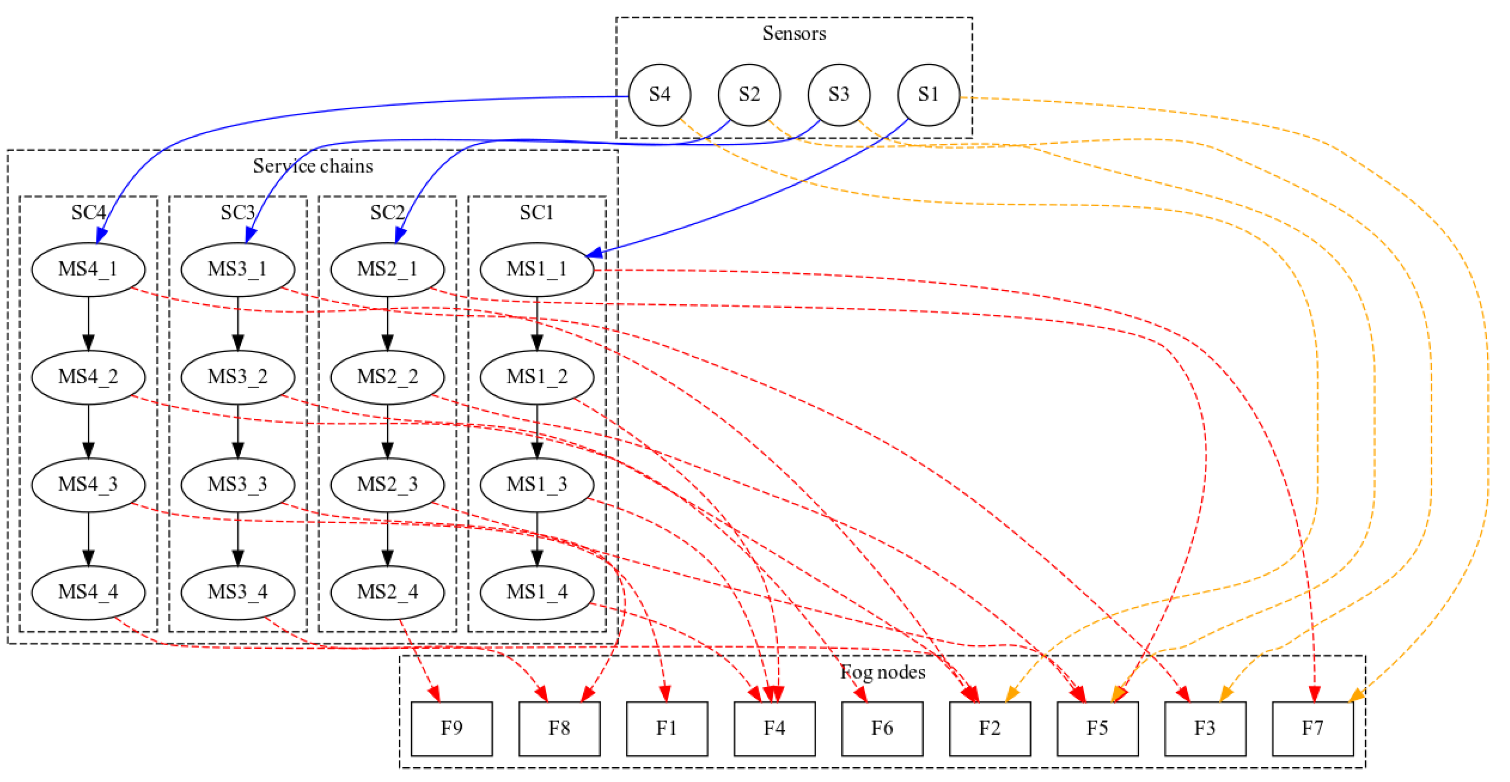
2.1. Reference Scenario

The fog computing paradigm typically involves the deployment of services close to the source of data that needs to be processed or to the application’s end users. Unlike the cloud computing context, this scenario is characterized by high heterogeneity of resources such as computational capacity of nodes and network delays for inter nodes communications. We assume that fog nodes are computing nodes with a non-negligible computational capacity. Each node can provide several services concurrently, for example, by using containerized environments. To better explain our vision, consider fog nodes can be considered as similar to computing elements placed alongside mobile phone antennas, rather than battery-operated motes in a sensor network. In this context, we focus on the application microservice placement issue, that is, the problem of how to best allocate microservices on the distributed fog nodes with the objective of minimizing the application response time and satisfying the SLAs. The inputs to the problem are:
  • A list of applications with related SLAs;
  • A set of fog nodes, along with their computational capacity;
  • A demand for applications with short-to-mid term expected load that is known a priori.
We assume that microservices can be stateful, meaning that migrating or re-deploying them in a short time span is not feasible. Even if requests from a single client, i.e., a sensor or a user, are difficult to predict, we assume that the overall incoming request rate either remains stable through time or changes slowly. This means that the time frame for a service deployment is on the order of tens of minutes up to one hour, and that the system load can be considered constant for that time. It is worth noting that this provides an order of magnitude for the time needed to solve the optimization problem, that is, it should reach a solution within a time frame of minutes.
In this scenario, we assume that each IoT application is modeled as a microservice chain that consists of multiple (at least two) independent and interconnected microservices. Without loss of generality, we model a service chain c as an ordered sequence of microservices m i , i 1 , 2 , n . The microservice chain length is the number of microservices composing the chain.
As examples of applications that can be supported by our solution, we propose two chains of microservices. First, monitoring and logging of sensor data in an industrial plant. In this application (1), the chain is composed of (1a) data collection, (1b) data validation, (1c) data smoothing to remove outliers, (1d) alert triggering, and (1e) data logging. Second, traffic surveillance application based on smart traffic lights. In this case (2), the microservices are (2a) image collection, (2b) car identification, (2c) plate number recognition and anonymization, and (2d) data logging to a database.
The microservices in a service chain may be allocated over one or over multiple fog nodes, and a fog node may host microservices belonging to different service chains. Fog nodes may have different computational capabilities, and are interconnected with each other by means of heterogeneous high-speed network.
The final objective is to define an optimal microservice placement that meets applications’ SLAs. To this end, as a main performance metric we consider the application’s service response time, that is, the time passing between the end user request and the receipt of the application’s reply. This metric is influenced by different elements, with the following being the most important: (i) the application request load, (ii) the average service time of the microservices in the service chain, and (iii) the computing capability of the fog nodes. Furthermore, it is important to mention that the presence of chains of microservices may lead to higher levels of complexity in the concept of SLAs, for example, where issues about availability are concerned. In this paper, we focus on SLAs based on the average service time of the microservices composing the chain; however, more complex SLAs could be included in the model and evaluated in future works.
In the scientific literature, several studies have proposed mechanisms for service placement over the geographically distributed nodes of a fog infrastructure starting from the simplifying assumption that an IoT application consists of only a single microservice [17,18,19]. A lower number of studies have considered IoT applications modeled as microservice chains to be placed over the fog nodes. An example of such proposed solutions are those based on completely distributed approaches [20,21]. The study in [20] sought to optimize energy consumption and communication costs by exploiting a game-theoretic approximation approach. In [21], a cooperative scheme allowed fog nodes to identify the best amount of requests to be forwarded and processed by each other to improve the response time. On the other hand, a centralized approach was presented in [22], where the authors formulated a mixed-integer nonlinear programming problem with the objective of minimizing the completion time of applications by jointly considering task placement and scheduling.
In this paper, we focus on centralized approaches relying on heuristics able to cope with the nonlinear nature of the optimization problem used to minimize the response time of the service chains. One of the presented heuristics, based on Genetic Algorithms, was presented by the authors in our previous paper [5], while the other two heuristics are novel proposals to address the microservice placement problem in fog computing contexts. The proposed heuristics are described in detail in Section 3.

2.2. Problem Definition

We now define the problem of microservice placement in a fog computing infrastructure. In order to formalize the optimization problem, we introduce the symbols and notation in Table 1.
The goal of the optimization problem is to minimize the average response time of each service chain; thus, the objective function in Equation (1) is a weighted sum of the response time for every considered service chain. The weights w c , c C are chosen such that c w c = 1 . One possible approach, which we use in this paper, is to consider the weight of every service chain proportional to its activation frequency λ c , that is, w c = λ c / Λ with Λ = c λ c , although other solutions can be adopted without altering the general validity of the model.
min o b j ( X ) = c C w c R c
subject   to : f F x m , f = 1 m M ,
λ f S f < 1 f F ,
R c < T c S L A c C ,
x m , f = { 0 , 1 } , m M , f F ,
The optimization problem is characterized by three constants. Equation (2) means that every microservice is allocated to one and only one fog node. Equation (3) forces every fog node not to be in an overload condition ( λ f S f is the load on fog node f). The model can be extended to cope with additional constraints, such as available memory on the fog nodes or I/O limits; for the sake of simplicity, we focus here on a model with as few constraints as possible. The last model constraint, Equation (4), requires that the SLA of each service chain be respected. In this paper, we consider
T S L A = K · m c S m
where K is a coefficient.
The last constraint, Equation (5), captures the Boolean nature of the decision variable x m , f .
The objective function of the optimization problem requires a model for the response time of a service chain. To this end, we must consider that the invocation of a generic service chain c can be described as a sequence of the wait time, service time, and network delay for every fog node hosting a service belonging to that chain. Therefore, we can model the response time R c of service chain c, that is, the component of the sum in Equation (1), using Equation (7):
R c = m c f F x m , f · W f + m c S m + + m 1 , m 2 c f 1 , f 2 F o m 1 , m 2 · x m 1 , f 1 · x m 2 , f 2 · δ f 1 , f 2
where o m 1 , m 2 is the order of execution of microservices in c. In particular, o m 1 , m 2 = 1 m 1 m 2 , meaning that service m 1 is invoked just before service m 2 in the service chain.
It is worth noting that our simplified approach to describing network delay can be explained by considering that, in the reference scenario, fog nodes are connected with reliable network links. The network delay δ f 1 , f 2 can be expressed as the latency plus the transmission time. In modern networks (often called Long Fat Networks), latency can be on the order of milliseconds or tens of milliseconds even for high speed networks, while transmission time is the product of the available bandwidth (in the orders of tens or hundreds of MBit/s) and message length. Considering the OpenAPI standard in which most microservices consume JSON tuples, we assume the message length to be relatively small and scarcely variant, which explains our modeling choices.
The last part of the model concerns the waiting time W f on fog node f. For this, we must consider that a generic fog node hosting multiple microservices experiences a service time that is a mixture of distributions, each of which refers to a single microservice. The resulting waiting time can be expressed using the Pollaczek–Khinchin Equation (8):
W f = S f 2 + σ f 2 2 · λ f 1 λ f S f .
The service time of a mixture of distributions can be described using its mean value (Equation (9)) and standard deviation (Equation (10)):
S f = 1 P f · m M x m , f λ m λ f S m
σ f 2 = 1 P f 2 · m M x m , f λ m λ f ( S m 2 + σ m 2 ) S f 2
where λ f = m M x m , f λ m is the total incoming load on node f.
The underlying assumption of Equation (8) is that the product form can be used to describe the queuing system of the fog infrastructure. However, this assumption is not always valid. Indeed, in case where the service times of the involved microservices cannot be expressed through exponential distributions, the resulting arrival process cannot be defined with an exponential distribution. In such cases, a G/G/1 model should be used in Equation (8) instead of a M/G/1 model. Unfortunately, there are no closed-form solutions to represent the inter-arrival time of a queuing server following the G/G/1 model. An M/G/1 model approximating the system’s behaviour may be exploited in cases where multiple microservices are located on a fog node or where the service times of the microservices present a standard deviation close to the mean value. The presented performance model is accurate as long as the system is close to these assumptions.
In light of the previous observations, Equation (8) can be used to describe the microservice chain response time as the sum of the following contributions: the sum of waiting times on the fog nodes, sum of service times, and network delays due to data transfer among two subsequent microservices in the service chain.
To evaluate the performance of a microservice placement solution, in this paper we consider the following metrics:
  • Heuristic execution time;
  • Service chain response time;
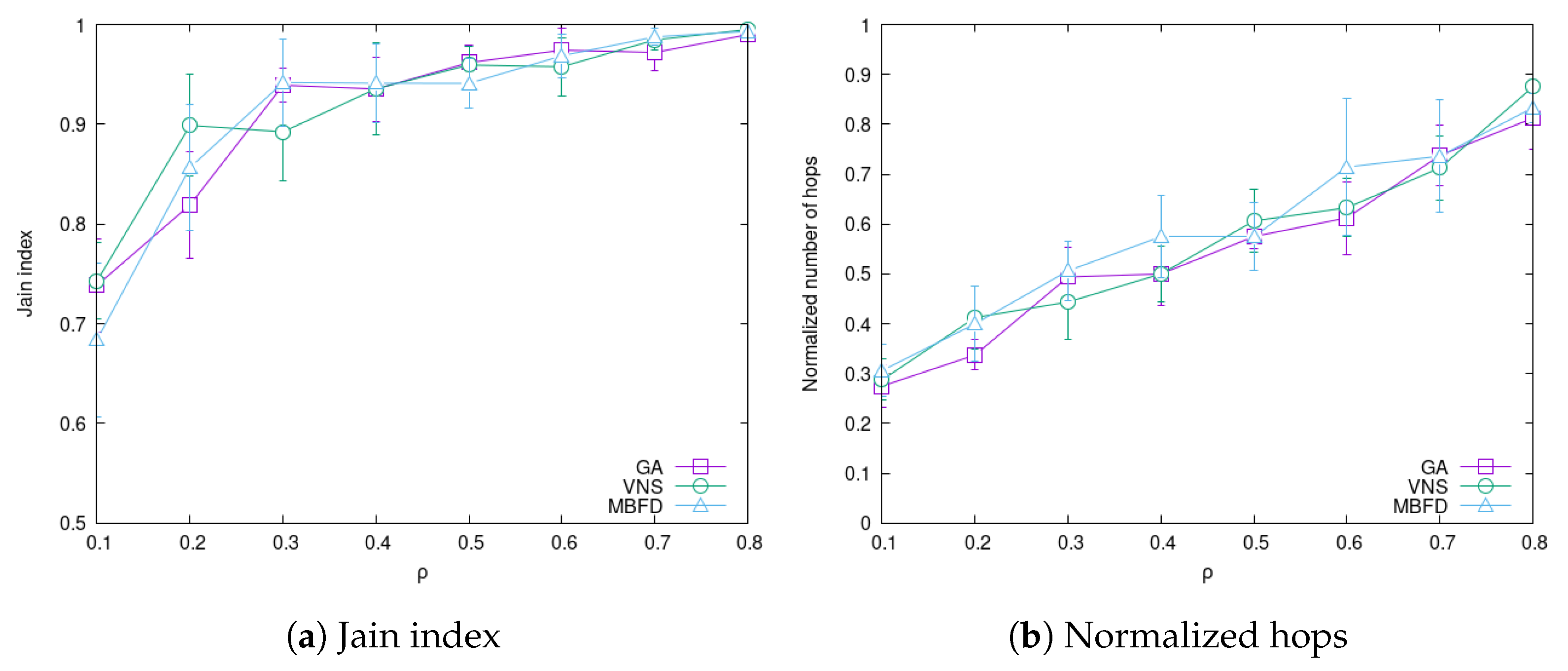
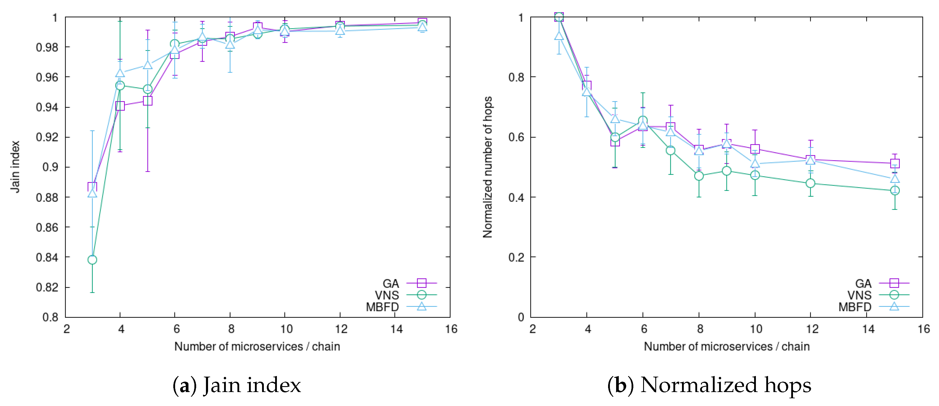
  • Number of hops normalized against the length of the service chain;
  • Jain index.
A detailed definition of the evaluation metrics is provided in Section 4.

3. Heuristics for Microservice Placement

In this section, we describe three heuristics for placing IoT application microservices over the nodes of a fog infrastructure. It is worth noting that we focus on algorithms based on a flat approach, which is typically suitable for cases in which a medium-sized set of fog nodes is involved in the placement solution. Indeed, considering a very large set of fog nodes when placing microservices of the same application chain would require a hierarchical or semi-hierarchical approach, which is typically not advisable due to the high latency between more distant fog nodes.

3.1. Modified Best Fit Decreasing

The Modified Best Fit Decreasing (MBFD) algorithm is a heuristic exploited in [11] to solve a server consolidation problem aimed at optimizing the placement of virtual machines on physical hosts for optimal energy and resource consumption. Because of the similar nature of the problem, we decided to implement an adapted version of MBFD to address the microservice allocation problem in fog computing infrastructures described in Section 2.2. In this adaptation, instead of mapping VMs onto hosts, microservices are mapped onto fog nodes.
As in the original algorithm [11], the adapted MBFD shown in Algorithm 1 follows a greedy approach.
The input structures are two lists that contain all the data of the fog nodes and microservices (e.g., fog node capacity) required to compute the solution. The main loop (defined in line 1) iterates on all the microservices ordered by mean service time; the motivation for this choice is to start the mapping process with the most demanding services. This is the same as in the original MBFD algorithm, and does not consider the impact of network delays in a distributed system.
Next (line 5–11), the algorithm iterates over the fog nodes, trying to place the microservice on each fog node. For every possible mapping, the SLA and the other constraints are checked to verify whether the solution is acceptable. In the case of an acceptable solution, the objective function is computed according to Equations (1) and (7). In this way, the best placement for that microservice is found and added to the solution being built. It is worth noting that the main difference from the original MBFD algorithm lies in the objective function. The objective function is the only part of the algorithm that considers network effects. Therefore, we expect this algorithm to provide higher quality solutions in cases where the network effect is not the main driver of optimal microservice placement.
Algorithm 1 Modified Best Fit Decreasing
INPUT:  m s L i s t : list of microservices, f o g L i s t : list of fog nodes
OUTPUT:  m a p p i n g : mapping of micro service over fog nodes
  1:
for  m s decreasing _ sort ( m s L i s t ) do
  2:
     m a p p i n g [ m s ] N o n e
  3:
     b e s t _ o b j N o n e
  4:
     n e w _ m a p p i n g m a p p i n g
  5:
    for  f f o g L i s t  do
  6:
          n e w _ m a p p i n g [ m s ] f
  7:
         if sla_ok( s o l u t i o n ) & constraints_ok( s o l u t i o n ) then
  8:
              o b j ← compute_obj_function( m a p p i n g )
  9:
             if  b e s t _ o b j = N o n e o b j < b e s t _ o b j  then
10:
                  m a p p i n g [ m s ] f
11:
                  b e s t _ o b j o b j
The C o m p u t e _ s o l u t i o n function (Algorithm 2) calculates the object function described in Section 2.2 based on the fog and chain parameters of the new mapping.
Finally, the algorithm determines whether n e w _ s o l u t i o n is a better solution by checking the following:
  • The Service Level Agreement is respected (4): this constraint is represented by the mean service time multiplied by a constant k (usually 10), as in Section 4.
  • Resources are used in a proper way: as an example, the remaining capacity of the fog nodes in a solution should not be less than zero.
  • The objective function in (1) in n e w _ s o l u t i o n is better than the older one in c u r r e n t _ s o l u t i o n ; as network delays are considered, MBFD can balance the placement using awareness of the delay between nodes.
The result of Algorithm 1 is the list of all microservices mapped over the fog nodes.
Algorithm 2 compute_obj_function
INPUT:  m a p p i n g : mapping of microservices on fog nodes
OUTPUT: Objective function for a given solution
for each f o g L i s t  do
     for each c h a i n L i s t  do
          if  Λ != 0 then
             calculate S f , σ f and R f
          else
              S f , σ f and R f all equals to 0
for each c h a i n L i s t  do
    calculate R c based on the m’s mapping
 calculate object function

3.2. Genetic Algorithms

Genetic Algorithms (GAs) are a class of heuristics used to solve a plethora of problems, including allocation problems in Edge and Fog computing [14,15].
The main characteristics of a genetic algorithm can be summarized as follows. A chromosome represents a solution modeled as a sequence of genes, where each gene represents a single parameter of the solution. The system starts from a population of individuals that are initially generated at random and then evolve through generations. Individuals represent possible problem solutions.
Considering the microservice allocation problem described in Section 2.2, a chromosome is set of M = M genes, where M is the number of considered microservices. The value of each gene is an integer number [ 1 , F ] , with F = F being the number of fog nodes. To map the decision variable x m , f on the genes, we can define the m t h gene as g m = { f : x m , f = 1 } . The proposed definition satisfies Equations (2) and (5), ensuring that a microservice m is allocated on one fog node and not more.
Each individual is associated with a fitness score that is calculated through the objective function (Equation (1)) and the evolution of the generations is guided by the individuals’ fitness scores. Due to constraints in (3) and (4) regarding the overload of fog nodes and the respect of SLAs, not every chromosome (solution) is acceptable. However, we prefer to let the population evolve while not excluding unacceptable solutions in order to exploit the capability of GAs to investigate a wide range of configurations. To take into account the two constraints, we choose to add corresponding penalty factors to the objective function, resulting in the following:
o b j * ( X ) = c C w c R c + P o l + P S L A
where P o l = S f * ( 1 + λ f 1 S f ) if overload occurs, with S f * being an arbitrary high value of the service time for a fog node. In a similar way, we define a penalty for SLA violations as P S L A = S c * ( S c / T S L A ) , with S c * representing an arbitrary high value of the service time of a microservice chain. The aim of the penalties is to eliminate individuals which violate the constraints. The choice to define both the penalties as proportional to the seriousness of the corresponding constraint violation is useful in cases where the population includes a great fraction of individuals with unacceptable values, as individuals with the worst values are the first to be eliminated.
The generations evolve by applying different genetic operators, such as mutation, crossover, and selection. We exploit a random mutation operator able to randomly modify a single gene in a chromosome; in this way, we can explore new possibilities in the solution space. Moreover, we apply a uniform crossover operator which combines two parent individuals into two new individuals. As a last step, we apply a tournament selection approach to identify individuals that should be included in the next generation based on their associated fitness score.
For the implementation of the algorithm, we rely on the DEAP (DEAP: Distributed Evolutionary Algorithms in Python library https://deap.readthedocs.io/en/master/, accessed on 24 June 2023). We tune the GA parameters through preliminary tests; specifically, the mutation probability is set to P m u t = 0.8 % and the crossover probability to P c x = 0.8 % . Moreover, we consider a population of 60 individuals with a number of generations equal to 600. This experimental setup is consistent with previous experiments in similar contexts [19].

3.3. Variable Neighborhood Search

The Variable Neighborhood Search (VNS) algorithm [16] is a metaheuristic optimization algorithm that aims to find high quality solutions to combinatorial optimization problems. It combines elements of the local search and diversification strategies to efficiently explore the solution space. The VNS algorithm works by iteratively improving candidate solutions through a combination of local search and perturbation. It starts with an initial solution, then performs a series of neighborhood explorations and improvements. At each iteration, it explores a nearby solution obtained by making small modifications to the current solution. The algorithm applies a local search procedure within each neighborhood to find the best solution within that neighborhood. If an improvement is found, the algorithm moves to that new solution. If no improvements are achieved, VNS introduces a perturbation in order to make more radical changes to the current solution. The target of this phase is to escape from the current local optima and explore new regions. In solving this problem, we use two structures for the local search and two structures for the perturbation phase:
  • N 1 Algorithm 3: randomly select a leaf node f 1 , the farthest microservice m 1 allocated to f 1 , the nearest fog node f 2 to m 1 , and the sensor m 2 allocated to f 2 nearest to f 1 . If this new solution is feasible, swap m 1 and m 2 from their respective fog nodes.
  • N 2 Algorithm 4: denote F o n as the set of active fog nodes; calculate the load of each fog node j F o n as r j = λ j μ j , then the average load of the active fog nodes as r ˜ = ( j F o n r j ) | F | . Randomly select f 1 F o n with load r 1 > r ˜ . Next, select the farthest microservice m 1 allocated to f 1 , then choose the node with the lowest load r 2 < r ˜ that is close to m 1 . Now, if feasible, remove m 1 from f 1 and place it on f 2 .
Algorithm 3 Group Close Sensors
Function Bring_Near(x)
f 1 R a n d o m l y S e l e c t F o g F r o m S o l u t i o n ( ) Random choose a fog node from the solution.
m 1 F a r t h e s t M i c r o s e r v i c e I n F 1 ( ) Get the farthest microservice allocated in F1.
f 2 C l o s e s t F o g T o M i c r o s e r v i c e ( ) Select the closest fog node to the selected microservice.
m 2 C l o s e s t M i c r o s e r v i c e T o F 1 ( ) Select the closest microservice from F1.
if  F e a s i b l e ( x , f 1 , f 2 , m 1 , m 2 )   then
      x S w a p ( x , f 1 , f 2 , m 1 , m 2 )  return  x
else
     return x
Algorithm 4 Load-Based Microservice Migration
Function Reduce_Load(x)
f o n G e t A c t i v e F o g N o d e s L i s t ( )
for  j 1 to | f o n |  do
     r j C o m p u t e N o d e L o a d ( )
r a v g C o m p u t e A v e r a g e L o a d ( )
f 1 R a n d o m l y S e l e c t B u s y N o d e ( ) Select fog node with load r ¯ > r
m 1 F a r t h e s t M i c r o s e r v i c e I n F 1 ( ) Get the farthest microservice allocated in F1.
f 2 G e t L o w e s t N e a r N o d e ( ) Select the node with lowest r ¯ < r a v g and near m 1
if  F e a s i b l e ( x , f 1 , f 2 , m 1 )   then
     x A l l o c a t e ( x , f 1 , f 2 , m 1 ) Remove m 1 from f 1 and allocate it on f 2 .
return  x
On the other hand, the structure used in the perturbation phase is as follows:
  • L 1 : perform every possible microservice exchange on the fog nodes.
  • L 2 : perform every possible allocation of microservices on the fog nodes.
The proposed VNS solution is represented as a recursive dictionary; each position represents a service chain and contains a dictionary that associates the microservice with the fog node on which it is located. A fog node that does not appear in any dictionary value is considered to be a turned-off node. The outer dictionary has a size | C | , while each position in the inner dictionary has a size | M C | . The initial solution of the VNS is created by allocating the microservices of the same chain to the same fog node.
When the initial solution is created, the objective function is calculated on the current solution. This is used to guide the VNS. A solution x is considered admissible with respect to the solution x if the objective function calculated on x is strictly lower than the objective function calculated on x.
The algorithm iterates over the set N k until no further improvement is possible during the descent phase using the L k structures. It terminates when no further improvements can be made. The solution tree is fully explored through systematic neighborhood changes, resulting in a global optimum for the proposed minimization problem at the end of the algorithm.

4. Experimental Results

4.1. Experimental Setup

In this section, we present a set of experiments aiming to assess the capability of the considered heuristics to find efficient solutions to the microservice placement problem in a fog infrastructure. To this end, we evaluate the effectiveness and efficiency of the previously proposed algorithms.
In order to perform our analysis, we generate several random problems with predefined characteristics and evaluate the time required to achieve a solution together with the quality of the solutions found by the different heuristics.
For this analysis, we relied on a virtualized system using XCP-NG as the hypervisor and running on an Intel Xeon Gold 6252 N CPU with a 2.30 GHz clock speed. The optimization algorithms were run on a VM with one vCPU and 8 GB of RAM (The presence of a single vCPU is not a problem for these algorithms, as they are not inherently parallel).
Figure 1 presents an example of a problem along with its deployment. The data flows in the logical organization of the services are represented by solid lines. The data flows from sensors to services are depicted in blue and the data exchanged by chained microservices in a service chain in black. The mapping of logical elements over the infrastructure is represented in dashed lines: yellow for links from sensors to the fog nodes and red for the deployment of services over the fog nodes.
Each problem is defined in terms of the following:
  • Service chain length L c , that is, the number of microservices composing a chain;
  • The service time of a service chain S c ;
  • The average network delay δ between two fog nodes;
  • Overall infrastructure load ρ ;
  • The problem size, that is, the number of fog nodes and service chains considered.
Throughout this analysis, as an efficiency metric we consider the time required to solve a problem; the quality of the solution is represented by several metrics. The most straightforward metric is the the response time of the service chains. However, to provide a deeper understanding of the solution, we additionally consider the average number of hops in the chain deployments normalized against the chain length (with a range of [ 0 , 1 ] ). Another critical performance metric of interest is the Jain index, a fairness measure that quantifies the ability of the genetic algorithm to achieve load balancing over the fog infrastructure. The Jain index is defined as J = 1 / ( 1 + CoV ( ρ f ) 2 ) , where ρ f is the utilization of each node f F and CoV ( · ) is the coefficient of variation, i.e., the ratio between standard deviation and mean, computed over all fog nodes. An index of 1 means perfect balancing, while a lower value means that the load is unevenly distributed among the fog nodes.
In this analysis, we consider chains of equal length, that is, L c = | { m c } | is constant c C . The impact of this parameter is evaluated in Section 4.4. In the other analyses, we consider chains composed of five microservices.
The overall system load is defined as
ρ = c λ c L c · c S c f P f ,
which means that the loads have ranges in the interval ρ [ 0 , 1 ] . The impact of this parameter is studied in Section 4.3. In the other analyses we fix ρ = 0.6 , which corresponds to medium utilization of the infrastructure.
Concerning the problem size and according to the notation introduced in Table 1, the number of nodes can be identified as | F | , while the number of chains is | C | . As default values used unless otherwise specified, we consider a set of ten fog nodes supporting four service chains.
For this analysis, we assume that the SLA is set to 10 × the service time of the chain, which is a common value used in cloud applications; i.e., in Equation (6), we consider K = 10 . In our experiments, this SLA is automatically satisfied as long as no overload occurs, motivating our choice to not perform any specific analysis with respect to this parameter.

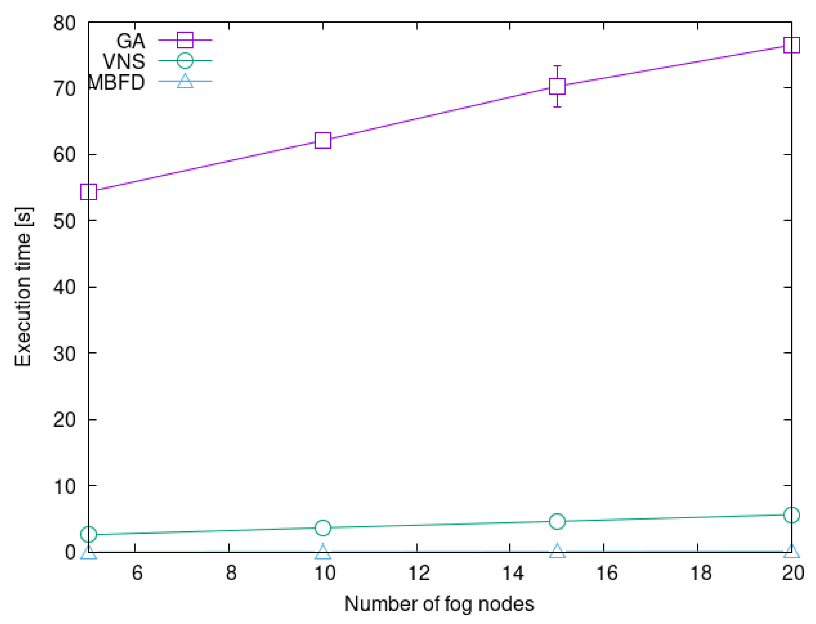
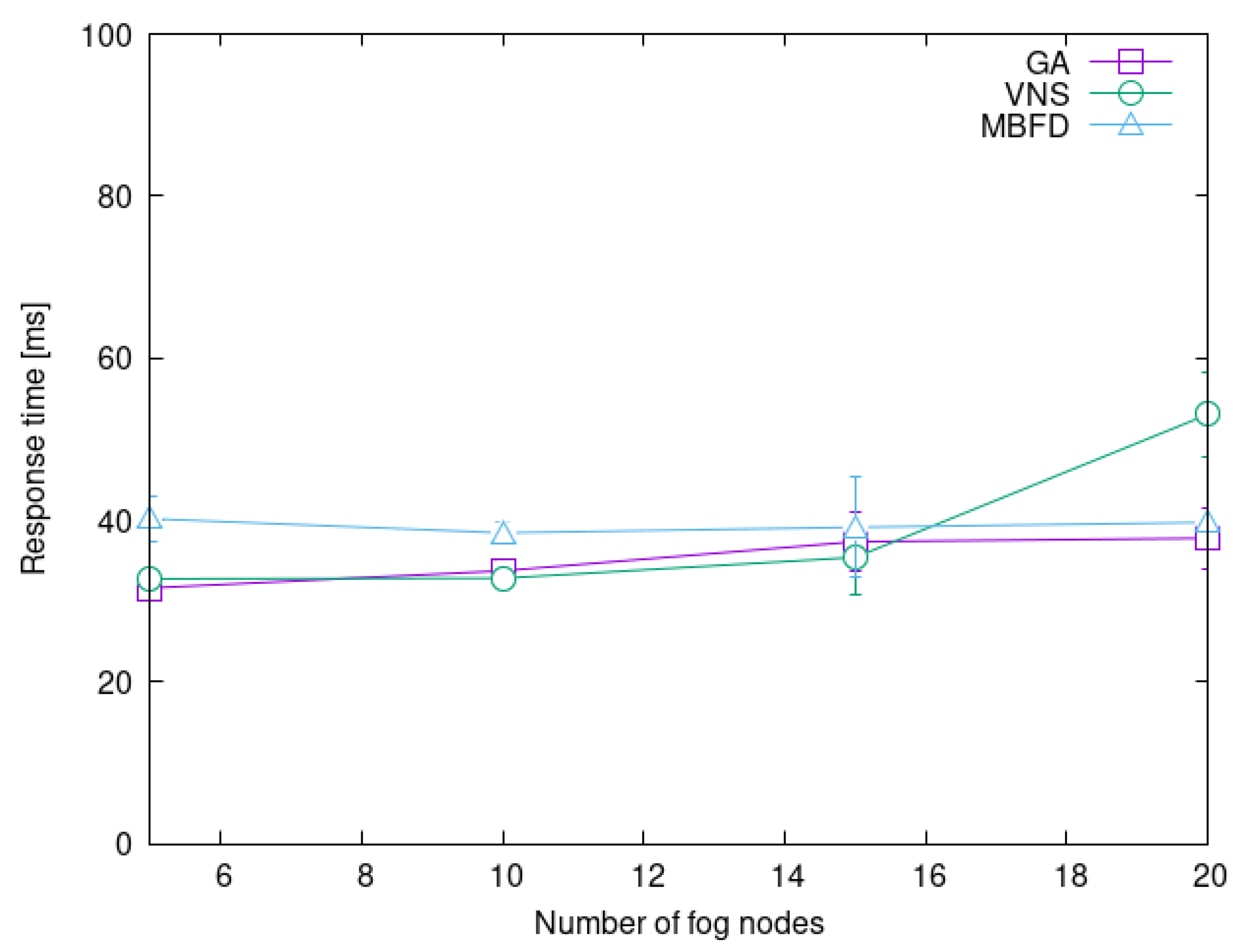
4.2. Heuristic Scalability

The first test aims to evaluate the ability of the proposed algorithms to scale with the problem size.
In Figure 2, we present a comparison of the heuristics’ execution time as a function of the number of fog nodes. Here, it is worth recalling that in order to keep the load even, we increase the number of service chains to be allocated along with the number of fog nodes.
A first result is the clearly different execution times of the various algorithms. The genetic algorithm is significantly slower than the alternatives, with an execution time roughly in the interval of 50–80 s as the problem size increases. The response time for the VNS algorithm is always below 10 s, and the execution time for the MBFD heuristic is almost negligible.
The poor performance of the GA heuristic is related to the large population of individuals used to explore the solution space and the large number of generations used to converge towards a solution. The VNS algorithm instead limits the number of solutions to be explored by defining small neighborhoods that can be explored quickly. Indeed, the execution time of the VNS algorithm only depends on the service chain length. Finally, the greedy heuristic of the MBFD algorithm is extremely fast, as it does not need to iterate over multiple possible solutions nor let a population evolve through generations.
For every algorithm, the execution time grows linearly with the problem size, that is, the number of nodes and the number of service chains considered. This can be explained by considering that the evaluation of the objective function requires a time that increases linearly with the problem size due to the summations in Equations (1) and (7).
A second aspect related to scalability is the stability of the solution quality with respect to the problem size. Figure 3 evaluates the response time of the solutions of the different algorithms as a function of the problem size.
It can be observed that the MBFD algorithm provides stable performance with a response time that does not change with the problem size. On the other hand, the genetic algorithm and the VNS algorithms suffer a degradation in the quality of the solutions as the problem size grows due to the small size of the solution space that the algorithms are able to explore. The problem is particularly evident for the VNS algorithm, which is outperformed even by the MBFD heuristic.

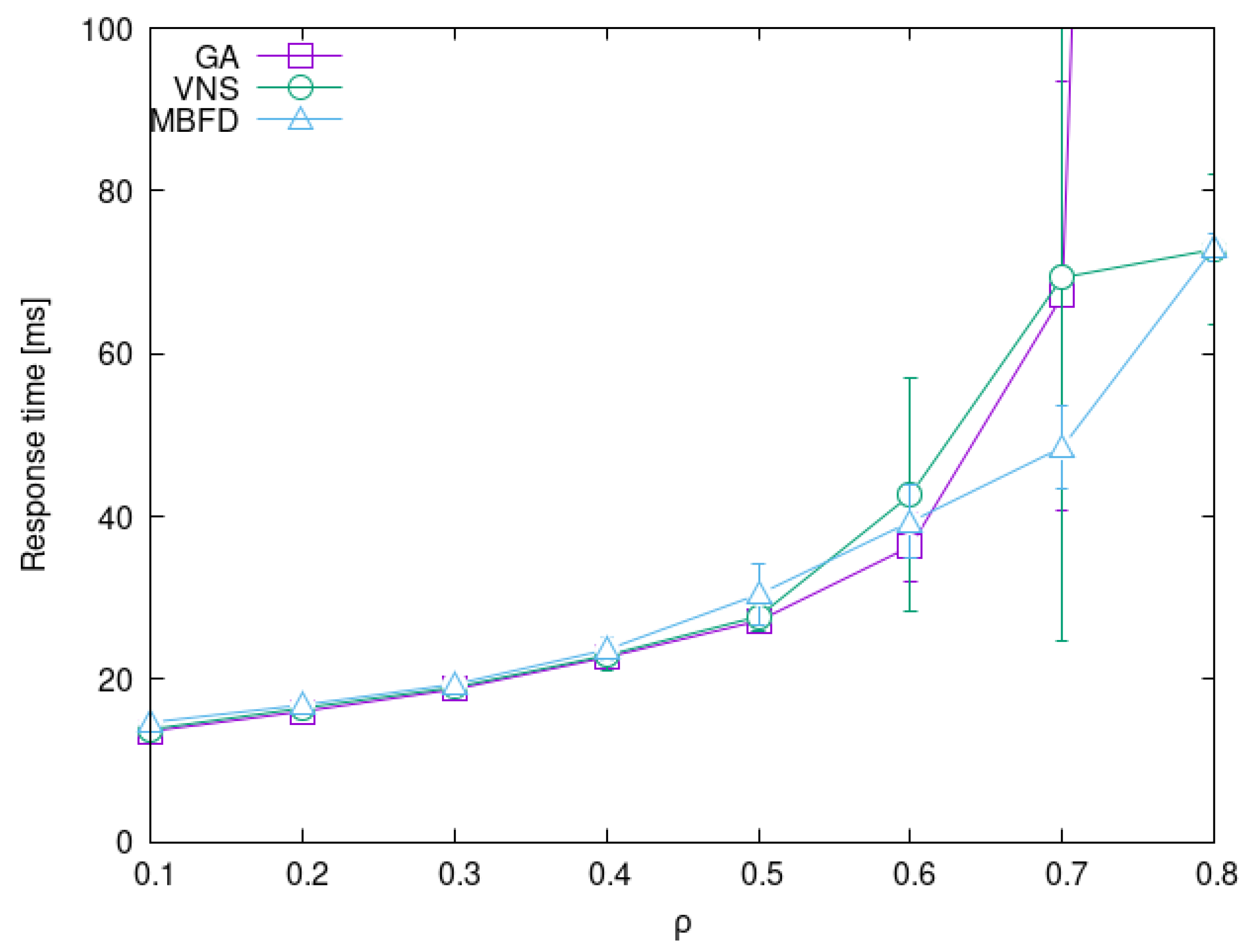
4.3. Impact of System Load

We now evaluate the quality of the solutions provided by the different algorithms. The first analysis concerns the impact of the system load ρ on the solution response time.
Figure 4 shows the average response time and its variance over the repeated experiments as a function of the global system load ρ . It can be observed that the performance of the proposed solutions are absolutely comparable for low values of ρ . As the utilization increases, we observe a growth in the response time and the variance of the value over different iterations. This result is compatible with previous studies based only on GAs [5].
The MBFD algorithm provides remarkably good performance in high load conditions. The reasons behind this behavior can be explained from the graphs in Figure 5. In particular, in Figure 5a it can be observed that the Jain index is generally good for every value of ρ . For MBFD this is natural, as the algorithm is explicitly designed to guarantee good load balancing, ensuring good performance even if the algorithm does not explicitly the global response time take into account. At the same time, in Figure 5b the number of hops increases for every algorithm as the load grows. This occurs because it becomes more and more difficult to place the microservices close one to the other as the risk of incurring overload increases.

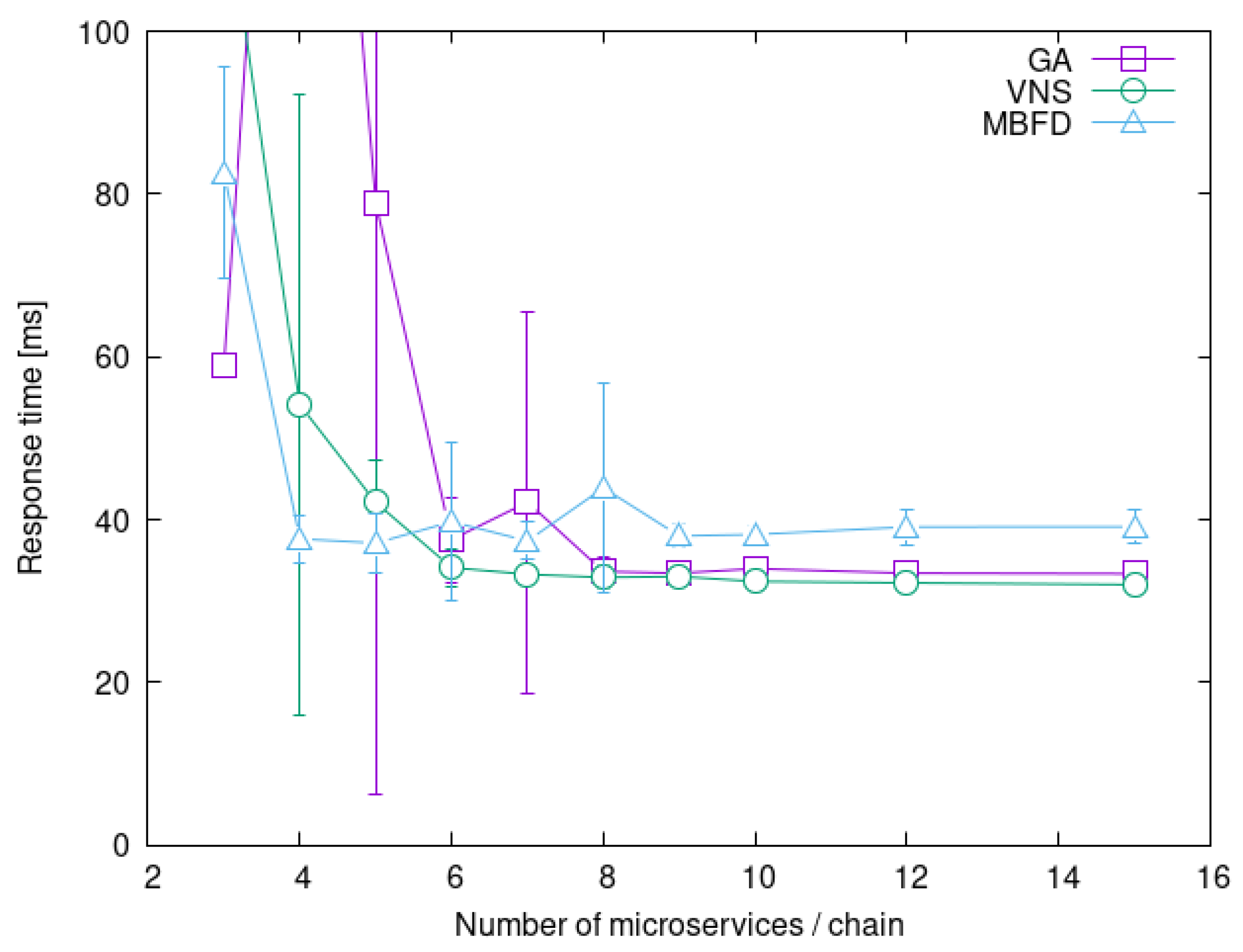
4.4. Impact of Service Chain Length

Another evaluation of the solution quality concerns how the response time of a solution depends on the service chain length.
In Figure 6, it can be observed that the response time and its variance both decrease as the length of the service chain grows. This effect has been pointed out in [5], and is due to the presence of large microservices that can bring a fog node close to the overload condition even on their own.
This effect can be observed in Figure 7a as well, where the Jain index is quite low for short service chains. Again, we observe that the load balancing approach of the MBFD algorithm provides good load balancing even in the case of short service chains (i.e., the blue line is higher than the other lines in the leftmost part of the graph), explaining the relatively low response time in Figure 6. At the same time, from Figure 7b it can be observed that the MBFD algorithm is not very effective at reducing the number of hops to avoid unnecessary network delays, as shown by the blue line in the graph. In a similar manner, the genetic algorithm does not perform well from this point of view due to the large space to be explored and its completely random approach to exploration of the solution space. Instead, the VNS algorithm, takes advantage of the neighborhood definition based on the problem characteristic, and can provide fast and accurate searching of the solution space, as indicated by the high Jain index in Figure 7a, and the low number of hops in Figure 7b, which together explain the low response time in Figure 6.

4.5. Summary of Experiments

Throughout our experiments, we evaluated the time required by each algorithm to solve the problem, with the MBFD heuristic being the fastest by at least one order of magnitude compared to VNS and GA being the slowest at one order of magnitude slower than VNS. The fast execution of MBFD results in lower quality results, with an average response time that can be nearly 30% higher compared to the best solution found. As the problem size grows, the GA and VNS heuristics tend to have worse performance, with VNS providing the worst quality solutions for large problems (+40% response time). It can be observed that as the the average load on the infrastructure grows, the MBFD heuristic outperforms the other approaches thanks to its focus on load balancing. This effect is additionally observed when short chains of microservices can lead to significant load unbalancing.
To summarize, while GA is the slowest to find a solution, it provides quite stable performance. While VNS is significantly faster than GA, it can provide poor quality solutions for large problems. Finally, MBFD is the fastest to obtain a solution and its load balancing-oriented operation ensures high quality solutions when load balancing is a critical factor, such as when the whole infrastructure is in a condition of high load or when certain heavy microservices can on their own determine a near-overload condition on a fog node, such as in the case of short microservice chains.

5. Conclusions

Assuming IoT applications modeled as chains of microservices, we propose a comparison of heuristics to optimize the placement of microservices over the nodes of a fog infrastructure. Our model considers both the network delay effect and the impact of computational load over the achieved performance while taking into account the inherent heterogeneity in the service time of the various microservices and in the computation power of each fog node. A thorough experimental evaluation was carried out considering different metrics such as the response time of the service chain, the average number of hops in the chain deployments, and the Jain index to measure the achieved load balancing among the fog nodes, with a final goal of understanding which heuristic is better suited to specific scenarios. Our future research directions span both modeling of complex problems and SLA formulations and evaluation to test our approach with realistic fog applications through small-scale prototypes and large-scale simulations.

Author Contributions

Conceptualization, C.C. and R.L., Software: C.G., R.L. and F.S.; Investigation: C.C., R.L., and F.S.; Writing: C.C., C.G., R.L., and F.S. All authors have read and agreed to the published version of the manuscript.

Funding

This research received no external funding.

Data Availability Statement

Data concerning experimental results can be requested from the authors.

Conflicts of Interest

The authors declare no conflict of interest.

References

  1. Bugshan, N.; Khalil, I.; Moustafa, N.; Rahman, M.S. Privacy-Preserving Microservices in Industrial Internet-of-Things-Driven Smart Applications. IEEE Internet Things J. 2023, 10, 2821–2831. [Google Scholar] [CrossRef]
  2. De Iasio, A.; Furno, A.; Goglia, L.; Zimeo, E. A Microservices Platform for Monitoring and Analysis of IoT Traffic Data in Smart Cities. In Proceedings of the 2019 IEEE International Conference on Big Data (Big Data), Los Angeles, CA, USA, 9–12 December 2019; pp. 5223–5232. [Google Scholar] [CrossRef]
  3. Al-Dhuraibi, Y.; Paraiso, F.; Djarallah, N.; Merle, P. Elasticity in Cloud Computing: State of the Art and Research Challenges. IEEE Trans. Serv. Comput. 2018, 11, 430–447. [Google Scholar] [CrossRef]
  4. Abdullah, M.; Iqbal, W.; Berral, J.L.; Polo, J.; Carrera, D. Burst-Aware Predictive Autoscaling for Containerized Microservices. IEEE Trans. Serv. Comput. 2022, 15, 1448–1460. [Google Scholar] [CrossRef]
  5. Canali, C.; Di Modica, G.; Lancellotti, R.; Scotece, D. Optimal placement of micro-services chains in a Fog infrastructure. In Proceedings of the 12nd International Conference on Cloud Computing and Services Science, CLOSER 2022, Tuzla, Bosnia and Herzegovina, 6–9 April 2022. [Google Scholar]
  6. Sarkar, S.; Chatterjee, S.; Misra, S. Assessment of the Suitability of Fog Computing in the Context of Internet of Things. IEEE Trans. Cloud Comput. 2018, 6, 46–59. [Google Scholar] [CrossRef]
  7. Yousefpour, A.; Ishigaki, G.; Jue, J.P. Fog Computing: Towards Minimizing Delay in the Internet of Things. In Proceedings of the 2017 IEEE International Conference on Edge Computing (EDGE), Honolulu, HI, USA, 25–30 June 2017; pp. 17–24. [Google Scholar] [CrossRef]
  8. Songhorabadi, M.; Rahimi, M.; MoghadamFarid, A.; Haghi Kashani, M. Fog computing approaches in IoT-enabled smart cities. J. Netw. Comput. Appl. 2023, 211, 103557. [Google Scholar] [CrossRef]
  9. Bonomi, F.; Milito, R.; Zhu, J.; Addepalli, S. Fog Computing and Its Role in the Internet of Things. In Proceedings of the First Edition of the MCC Workshop on Mobile Cloud Computing, MCC ’12, New York, NY, USA, 17 August 2012; pp. 13–16. [Google Scholar]
  10. Salaht, F.A.; Desprez, F.; Lebre, A. An Overview of Service Placement Problem in Fog and Edge Computing. ACM Comput. Surv. 2020, 53, 1–35. [Google Scholar] [CrossRef]
  11. Beloglazov, A.; Abawajy, J.; Buyya, R. Energy-aware resource allocation heuristics for efficient management of data centers for cloud computing. Future Gener. Comput. Syst. 2012, 28, 755–768. [Google Scholar] [CrossRef]
  12. Canali, C.; Lancellotti, R. Exploiting Classes of Virtual Machines for Scalable IaaS Cloud Management. In Proceedings of the 4th Symposium on Network Cloud Computing and Applications (NCCA), Munich, Germany, 11–12 June 2015. [Google Scholar]
  13. Shojafar, M.; Canali, C.; Lancellotti, R.; Abolfazli, S. An Energy-aware Scheduling Algorithm in DVFS-enabled Networked Data Centers. In Proceedings of the 6th International Conference on Cloud Computing and Services Science (CLOSER), Rome, Italy, 23–25 April 2016. [Google Scholar]
  14. Binitha, S.; Sathya, S.S. A survey of bio inspired optimization algorithms. Int. J. Soft Comput. Eng. 2012, 2, 137–151. [Google Scholar]
  15. Yusoh, Z.I.M.; Tang, M. A penalty-based genetic algorithm for the composite SaaS placement problem in the Cloud. In Proceedings of the IEEE Congress on Evolutionary Computation, Barcelona, Spain, 18–23 July 2010; pp. 1–8. [Google Scholar] [CrossRef]
  16. Hansen, P.; Mladenović, N.; Moreno Pérez, J.A. Variable neighbourhood search: Methods and applications. Ann. Oper. Res. 2010, 175, 367–407. [Google Scholar] [CrossRef]
  17. Yu, R.; Xue, G.; Zhang, X. Application Provisioning in FOG Computing-enabled Internet-of-Things: A Network Perspective. In Proceedings of the IEEE INFOCOM 2018—IEEE Conference on Computer Communications, Honolulu, HI, USA, 16–19 April 2018; pp. 783–791. [Google Scholar] [CrossRef]
  18. Skarlat, O.; Nardelli, M.; Schulte, S.; Dustdar, S. Towards QoS-Aware Fog Service Placement. In Proceedings of the 2017 IEEE 1st International Conference on Fog and Edge Computing (ICFEC), Madrid, Spain, 14–15 May 2017; pp. 89–96. [Google Scholar] [CrossRef]
  19. Canali, C.; Lancellotti, R. A Fog Computing Service Placement for Smart Cities based on Genetic Algorithms. In Proceedings of the International Conference on Cloud Computing and Services Science (CLOSER 2019), Heraklion, Greece, 2–4 May 2019. [Google Scholar]
  20. Kayal, P.; Liebeherr, J. Distributed Service Placement in Fog Computing: An Iterative Combinatorial Auction Approach. In Proceedings of the 2019 IEEE 39th International Conference on Distributed Computing Systems (ICDCS), Dallas, TX, USA, 7–9 July 2019; pp. 2145–2156. [Google Scholar] [CrossRef]
  21. Xiao, Y.; Krunz, M. QoE and power efficiency tradeoff for fog computing networks with fog node cooperation. In Proceedings of the IEEE INFOCOM 2017—IEEE Conference on Computer Communications, Atlanta, GR, USA, 1–4 May 2017; pp. 1–9. [Google Scholar] [CrossRef]
  22. Zeng, D.; Gu, L.; Guo, S.; Cheng, Z.; Yu, S. Joint Optimization of Task Scheduling and Image Placement in Fog Computing Supported Software-Defined Embedded System. IEEE Trans. Comput. 2016, 65, 3702–3712. [Google Scholar] [CrossRef]
Figure 1. Example of the generated problem.
Algorithms 16 00441 g001
Figure 2. Heuristic execution times.
Algorithms 16 00441 g002
Figure 3. Response time vs. infrastructure size.
Algorithms 16 00441 g003
Figure 4. Response time vs. system load ρ .
Algorithms 16 00441 g004
Figure 5. Impact of the system load ρ .
Algorithms 16 00441 g005
Figure 6. Response time vs. service chain length.
Algorithms 16 00441 g006
Figure 7. Impact of service chain length.
Algorithms 16 00441 g007
Table 1. Notation and parameters for the proposed model.
Model Parameters
M Set of microservices
F Set of fog nodes
C Set of service chains
λ m Incoming rEquation rate to microservice m
λ f Incoming rEquation rate to fog node f
λ c Incoming rEquation rate to service chain c
Λ Incoming global request rate
S m Avg. service time for microservice m
σ m Standard deviation of S m
P f Computational power of fog node f
W f Avg. waiting time on fog node f
S f Avg. service time on fog node f
σ f Standard deviation of S m
R f Avg. response time for fog f
R c Avg. response time for service chain c
T c S L A SLA of service chain c
o m 1 , m 2 Services order of execution in a chain
δ f 1 , f 2 Network delay between nodes f 1 and f 2
Model indices
fFog node
cService chain
mMicroservice
Decision variables
x m , f Allocation of microservice m to fog node f
Disclaimer/Publisher’s Note: The statements, opinions and data contained in all publications are solely those of the individual author(s) and contributor(s) and not of MDPI and/or the editor(s). MDPI and/or the editor(s) disclaim responsibility for any injury to people or property resulting from any ideas, methods, instructions or products referred to in the content.

