Article

A Plant Disease Classification Algorithm Based on Attention MobileNet V2

1
Xi’an Institute of Optics and Precision Mechanics, Chinese Academy of Sciences, Xi’an 710119, China
2
State Key Laboratory of Resources and Environment Information System, Institute of Geographic Sciences and Natural Resources Research, Chinese Academy of Sciences, Beijing 100101, China
3
Key Laboratory of Low Altitude Geographic Information and Air Route, Civil Aviation Administration of China, Beijing 100101, China
4
The Research Center for UAV Applications and Regulation, Chinese Academy of Sciences, Beijing 100101, China
*
Author to whom correspondence should be addressed.
Algorithms 2023, 16(9), 442; https://doi.org/10.3390/a16090442
Submission received: 24 August 2023 / Revised: 10 September 2023 / Accepted: 12 September 2023 / Published: 13 September 2023
(This article belongs to the Special Issue Algorithms for Smart Cities)

Abstract

:
Plant growth is inevitably affected by diseases, and one effective method of disease detection is through the observation of leaf changes. To solve the problem of disease detection in complex backgrounds, where the distinction between plant diseases is hindered by large intra-class differences and small inter-class differences, a complete plant-disease recognition process is proposed. The process was tested through experiments and research into traditional and deep features. In the face of difficulties related to plant-disease classification in complex backgrounds, the advantages of strong interpretability of traditional features and great robustness of deep features are fully utilized, and include the following components: (1) The OSTU algorithm based on the naive Bayes model is proposed to focus on where leaves are located and remove interference from complex backgrounds. (2) A multi-dimensional feature model is introduced in an interpretable manner from the perspective of traditional features to obtain leaf characteristics. (3) A MobileNet V2 network with a dual attention mechanism is proposed to establish a model that operates in both spatial and channel dimensions at the network level to facilitate plant-disease recognition. In the Plant Village open database test, the results demonstrated an average SEN of 94%, greater than other algorithms by 12.6%.

1. Introduction

With the proliferation of artificial-intelligence technology, the development of smart agriculture has gained momentum. In the area of plant-disease recognition, researchers have conducted much research, which can be divided into two approaches: classification and clustering.
Classification perspective: Based on the analysis of inter-class differences, plant-disease classification can be mainly divided into traditional-feature and deep-feature aspects. Representative algorithms based on traditional features include: Al-Hiary et al. [1] analyzed the typical characteristics of plants and proposed a fast classification algorithm for plants; Kulkarni et al. [2] constructed a classifier founded on texture features extracted from plant images; Arivazhagan et al. [3] classified plant health status based on texture features; Hossain et al. [4] achieved plant-disease classification through leaf color information analysis; Singh et al. [5] implemented swift plant-disease detection from the algorithmic level based on image segmentation and soft computing techniques; Kaur et al. [6] implemented plant-disease detection based on gradient and texture features; Nanehkaran et al. [7] formulated a visual model for disease analysis and correlation assessment; Pujari et al. [8] extracted plant image features based on SVM and ANN; Brahimi et al. [9] focused on the salient area of plants, established a saliency map, and achieved plant-disease classification; Mahmoud et al. [10] established a disease image representation using inverse coding technology; and Sandesh et al. [11] constructed an Adaboost-based model for disease prediction from the perspective of color. Representative algorithms based on deep feature extraction mainly include: Hang et al. [12] proposed a CNN-based method for plant-disease analysis; Atila et al. [13] devised an EfficientNet deep learning model to mine image depth features; Sardogan et al. [14] conducted research based on CNN with LVQ algorithm; Deepa et al. [15] enhanced images and established an interactive model to facilitate disease classification; ALTAN et al. [16] constructed capsule networks to measure the efficacy in plant-disease classification; Pal et al. [17] established the semantic relationship between images and diseases in AgriDet; and Liang et al. [18] introduced a deep-learning network for plant-disease classification and severity assessment.
Clustering perspective: Models are built by an analysis of intra-class differences. Representative algorithms based on traditional features include: Yu et al. [19] constructed a K-means model to analyze intra-class differences and achieve clustering; Padol et al. [20] established an SVM to cluster different disease images; Rani et al. [21] enhanced clustering accuracy by adding SVM on top of the K-means algorithm; Trivedi et al. [22] established a model from the perspective of a color histogram for image analysis; Faithpraise et al. [23] established a K-means model for disease classification from a clustering perspective; Tamilselvi et al. [24] used unsupervised machine-learning algorithms to cluster based on color features; and Hasan et al. [25] proposed an extended kernel-density-estimation approach to analyze disease morphology. On the other hand, representative algorithms based on deep feature extraction mainly include: Yadhav et al. [26] obtained clustering features based on the CNN model with optimized activation functions; Bhimavarapu et al. [27] fused PSO and CNN algorithms to extract multi-dimensional features; Hatuwal et al. [28] experimentally demonstrated the capabilities of random forest, KNN, SVM, and CNN for clustering; Pareek et al. [29] established a 1D-CNN model for clustering based on image segmentation; Mukti et al. [30] achieved plant-disease detection based on multiple iterations of ResNet; Li et al. [31] analyzed plant diseases through the construction of the model ensemble with inception module and cluster algorithm; Türkoğlu et al. [32] used deep networks to extract disease image features and analyze differences between classes; and Ramesh et al. [33] constructed a model from the perspective of image and machine learning to achieve disease classification.
In summary, plant-disease classification algorithms based on images face the following issues: (1) Traditional algorithms are based on visual features that can be easily affected by natural factors, such as lighting and angles, with limited performance improvement. (2) Deep-learning algorithms based on neural conduction processes exhibit the features of strong robustness and positive effects. However, the classification effect remains to be improved in the face of complex background interference.
Through an analysis of the image features of plant diseases, traditional features with deep features are integrated to propose a comprehensive plant-disease feature classification algorithm, which involves the following components: (1) The OSTU algorithm based on the naive Bayes model is proposed to eliminate background interference and focus on the area where leaves are located. (2) From the perspective of traditional features, a multi-scale and multi-directional Gabor feature extraction model is proposed to obtain interpretable features. (3) Based on the advantages of MobileNet V2, spatial attention and channel attention mechanisms are proposed for plant-disease classification.
The remainder of this paper is organized as follows: Section 2 introduces the constructed database, including the multilevel feature extraction algorithm in Section 2.1 and the MobileNet algorithm based on dual attention in Section 2.2. Section 3 presents the experimental results and analysis, which verify the effectiveness of the proposed algorithm. Section 4 summarizes the innovations introduced in this paper and outlines potential avenues for future research.

2. Materials and Methods

The experimental data are sourced from the Plant Village public database provided by the University of Pennsylvania. It includes a total of 61 categories, classified by “species-disease-degree”. The categories consist of 10 species, 27 diseases (24 of which are classified as general or severe), and 10 health classifications, as shown in Table 1. The dataset comprises 31,718 pictures in the training set and 4514 pictures in the test set, as shown in Figure 1. We can see that there are certain similarities within classes and certain differences between classes. It is crucial to choose effective features.
The proposed plant disease classification algorithm based on an attention mechanism is shown in Figure 2. The algorithm comprises the following steps: (1) The OSTU algorithm based on the weighted Naive Bayes model is constructed to focus on the area where leaves are located and remove the influence of complex backgrounds. (2) Interpretable traditional features are adopted and extracted from multi-scale and multi-directional Gabor filters. (3) The extracted Gabor features are fed into a dual attention network for plant disease classification.

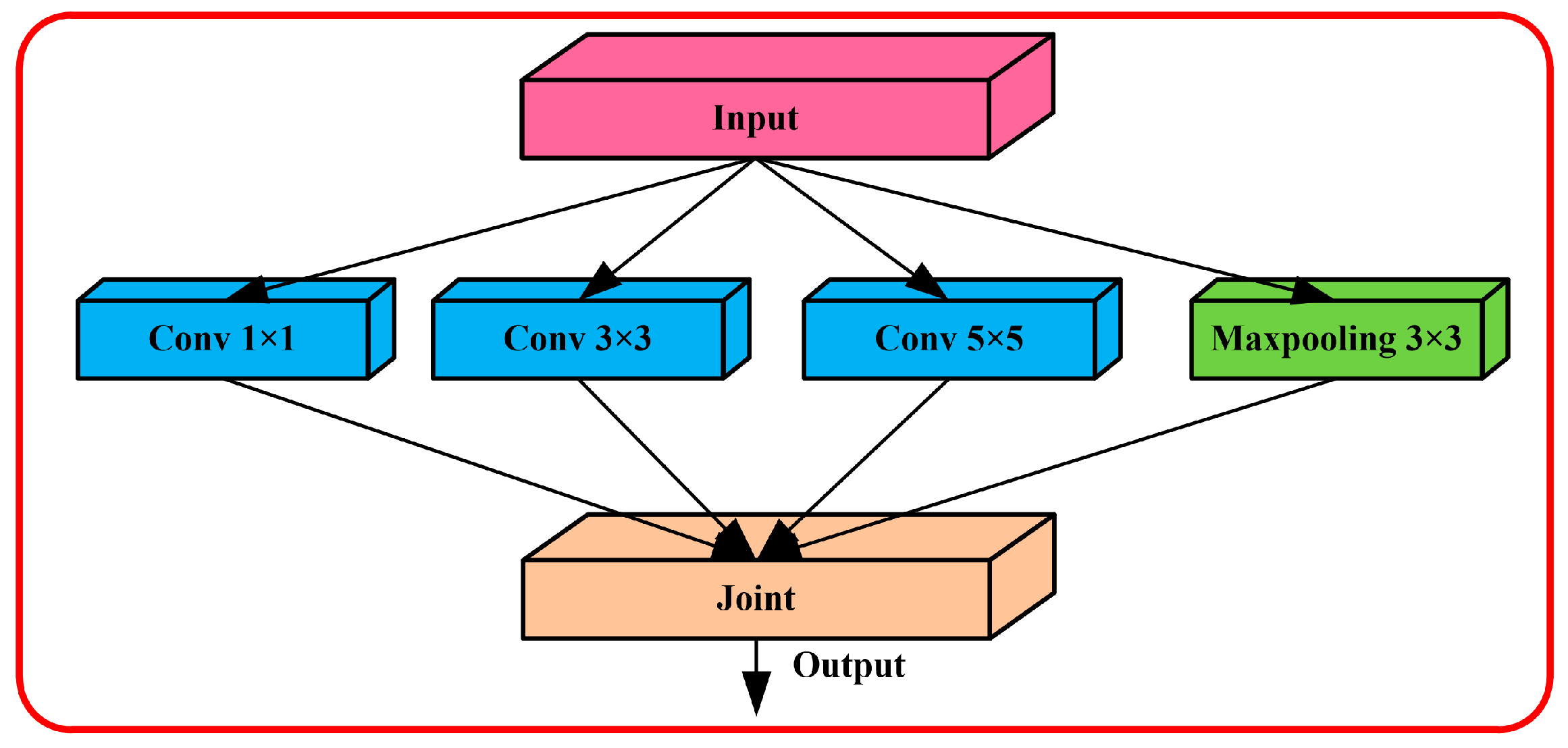
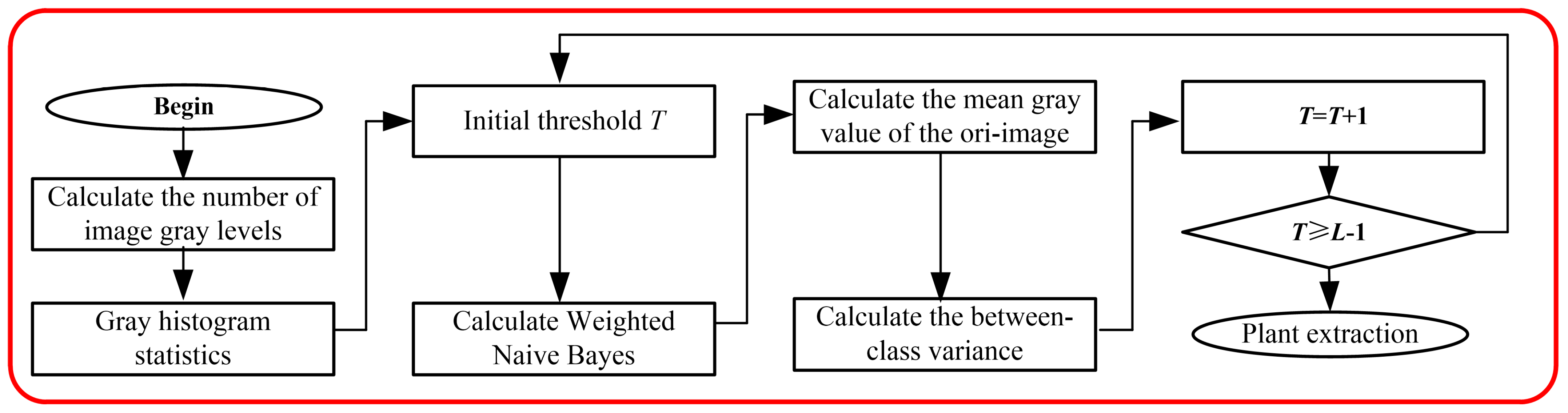
2.1. Multilevel Feature Extraction Algorithm

The OTSU algorithm [34] achieves image segmentation through the calculation of the image gray features to determine the threshold. The principle is to maximize the inter-class variance between the objects and the background of the image. It serves as an automatic optimization algorithm for image segmentation.
The total number of pixels in the image is notated as N, and the pixel gray level as G. fi represents the number of pixels at gray level i. The threshold t is selected to divide the analysis into two categories: C0 and C1. Then, the corresponding probability of the two categories can be expressed as:
w 0 = P C 0 = i = 1 t P i = w t             P i = f i / N w 1 = 1 w t
The inter-class variance of each pixel σ B 2 t is selected as the evaluation index:
σ B 2 t = μ r w t μ t 2 w t 1 w t
μ r = μ L = i = 1 L i P i ,             w t = i = 1 t P i
Then, the optimal threshold T is determined.
σ B 2 T = max 1 t l σ B 2 t
The traditional OTSU algorithm considers the neighborhood information. However, in cases where there is minimal distribution difference between background features and target pixels, the two peaks may not be clearly defined, resulting in a poor segmentation effect. To improve the traditional OTSU image processing method, the weighted Naive Bayes algorithm is introduced to refine the segmentation effect.
The naive Bayes algorithm is a commonly utilized data classification algorithm in machine learning algorithm research [35]. Thanks to its strong theoretical support, it boasts high classification efficiency and has been continuously studied and applied across different fields. Firstly, the Bayes principle is introduced:
P c X = P X c P C P X
where P(c|X) represents the posterior probability that X belongs to the category c. P(c) and P(X) denote the prior probabilities of category c, and conditional X. P(X|c) represents the posterior probability that category c belongs to the condition X.
Suppose the dataset comprises m attribute variables denoted as A, and the category variables are C = {c1, c2, … cn}. The Naive Bayes model is obtained
c x N B = arg max i P c k i = 1 m P x i c k ,             1 k n
where P(ck) is the prior probability when category c takes the value of k; P (xi|ci) represents the posterior probability that category ci belongs to the condition xi.
The traditional naive Bayes model presupposes that different attributes are independent of one another, which is difficult to achieve in practice. In cases where there is a correlation between certain attributes, it greatly reduces the classification efficiency of the model, resulting in inaccurate experimental results. Therefore, attribute weighting is employed to retain the high classification accuracy of the traditional naive Bayes algorithm. The approach also alleviates the negative impact caused by the special condition of attribute independence, which improves and enhances the efficiency of the traditional algorithm to a large extent. The corresponding formula is
c x P = arg max i P c k i = 1 m P x i c k w i ,             1 k n
where wi represents the weight value of the class attribute Ai, exerting control over the segmentation effect. The key to the improved classification algorithm lies in the precise determination of the corresponding weight value of each attribute to yield superior results.
Through the above algorithms, the segmentation problem is transformed into a problem in probability theory calculations. The segmentation image is obtained by isolating the gray features in the image data and training with the Naive Bayes model. The corresponding algorithm process is illustrated in Figure 3.
The input image gray map is notated as G, with a total of N pixels, and the gray levels i = 0, 1… L − 1. The corresponding gray histogram is represented as H = {h0, h1, … hL−1}. The threshold T is calculated to divide the gray image into Gb (background region) and Gf (foreground region). The corresponding probability distributions are
P G b = i = 0 T P i
P G f = i = T + 1 L 1 P i
The average occurrence probability of each gray level is given by:
M G b = i = 0 T i × w i × P i P G b
M G f = i = k + 1 L 1 i × w i × P i P G f
The threshold T to divide the original gray image into two categories is calculated by:
η = σ B 2 σ G 2
σ B 2 = P G b M G b M G 2 + P G f M G f M G 2
σ G 2 = i = 0 L 1 i M G 2 P i
The distance between classes of the two parts is calculated, and the distance is proportional to the segmentation effect. Therefore, the corresponding optimal threshold is:
T = max 0 i L 1 σ B 2
In order to analyze plant features, Gabor filtering [36] was introduced for further feature extraction. The Gabor filter, a kind of wavelet transform, exhibits excellent characteristics in the time and frequency domain. The Gabor function can be used to construct filters with different scales and directions. Since plant disease images are two-dimensional, research was conducted at the two-dimensional Gabor level. Its corresponding complex expression is as follows:
g x , y = exp X 2 + γ 2 Y 2 2 σ 2 exp i 2 π X λ + φ
X = x cos θ + y sin θ Y = x sin θ + y cos θ
g r e = exp X 2 + γ 2 Y 2 2 σ 2 cos 2 π X λ + φ g i m = exp X 2 + γ 2 Y 2 2 σ 2 sin 2 π X λ + φ
where θ is the filter direction, λ is the filter wavelength, φ is the phase translation, γ is the spatial aspect ratio, σ is the standard deviation of the Gaussian factor, and b is the bandwidth. gre represents the real part, and gim represents the imaginary part.
σ = λ π ln 2 2 2 b + 1 2 b 1
When the curve of the elliptic Gaussian envelope modulated by the complex sine wave of the Gabor function falls within the range of (µ − 3σ, µ + 3σ), the area contained accounts for about 99.7% of the total area.
When designing a deep network, the receptive field must cover the entire relevant image region and be large enough to capture the context information for each pixel axis. Currently, the mainstream algorithms stack either large convolution kernels in shallow or small convolution kernels. However, increasing the receptive field will lead to a rise in training parameters and the computational cost.
If the standard convolution layer contains K m × m convolution kernels and c input features, then the corresponding number of parameter training is (m × m × c + 1) × K. The proposed Gabor convolutional layer structure only requires updating of 4 parameters in each iteration, and the corresponding training parameter is (4 × c + 1) × K. Therefore, the Gabor convolution kernel is advantageous for the design of more compact networks.
In the Gabor convolution kernel, the parameters of each Gabor filter need to be optimized. The gradient descent algorithm is used to optimize filtering parameters through back propagation according to the objective function. The reverse derivation process is as follows:
g r e λ = π X λ 2 g i m g r e θ = g r e X Y σ 2 γ 2 1 2 π Y λ g i m g r e φ = g i m g r e σ = X 2 + γ 2 Y 2 σ 3 g r e g r e γ = γ 2 Y 2 σ 2 g r e
To further enhance the feature map expression, Gabor filter weighting is adopted to generate Gabor filter with U directions and V scales. The direction is weighted by learning the weight vector W. The modulation process is as follows:
C i , u v = C [ W g u , v ]
where u and v represent orientation and scale indexes. Since the Gabor filter contains multiple directions, the corresponding output feature updating process follows the back propagation mechanism:
δ = L C u n = u = 1 U L C u n W g u , v
C u n + 1 = C u n η δ
where L is the loss function, η is the learning rate, and C u n is the result of the nth iteration. This makes the model more compact and robust to changes in direction and scale.

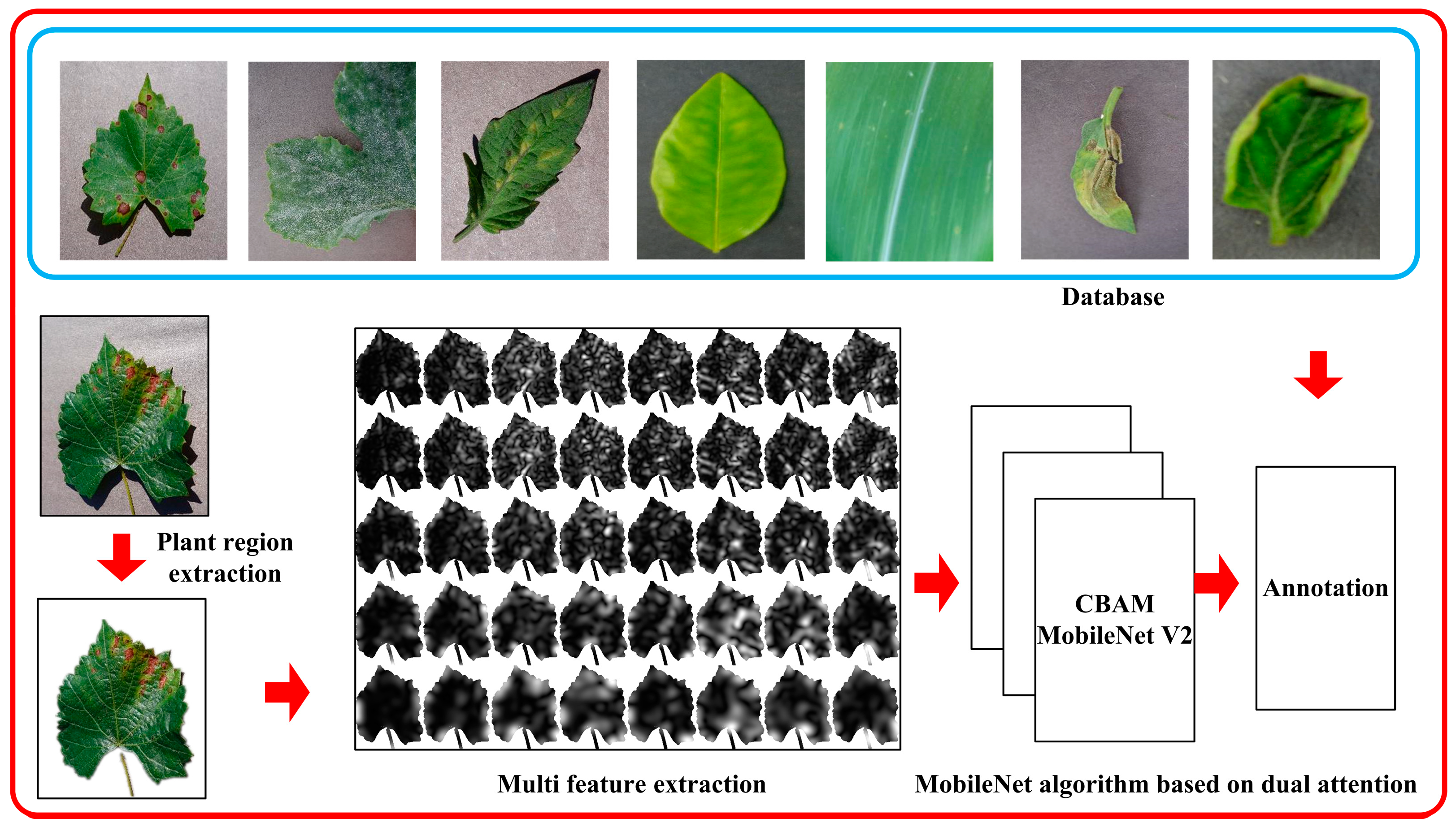
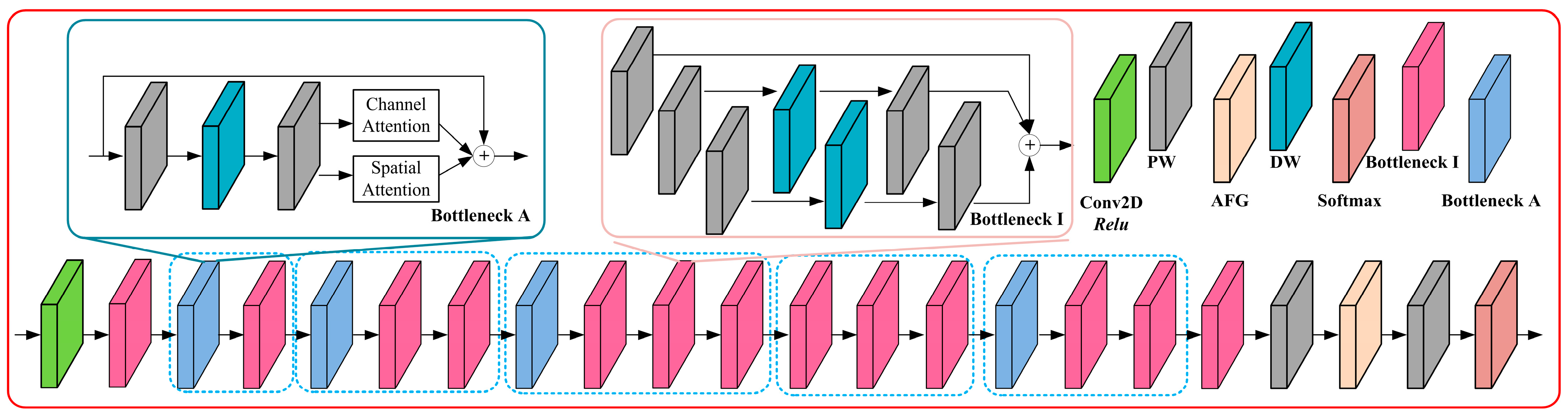
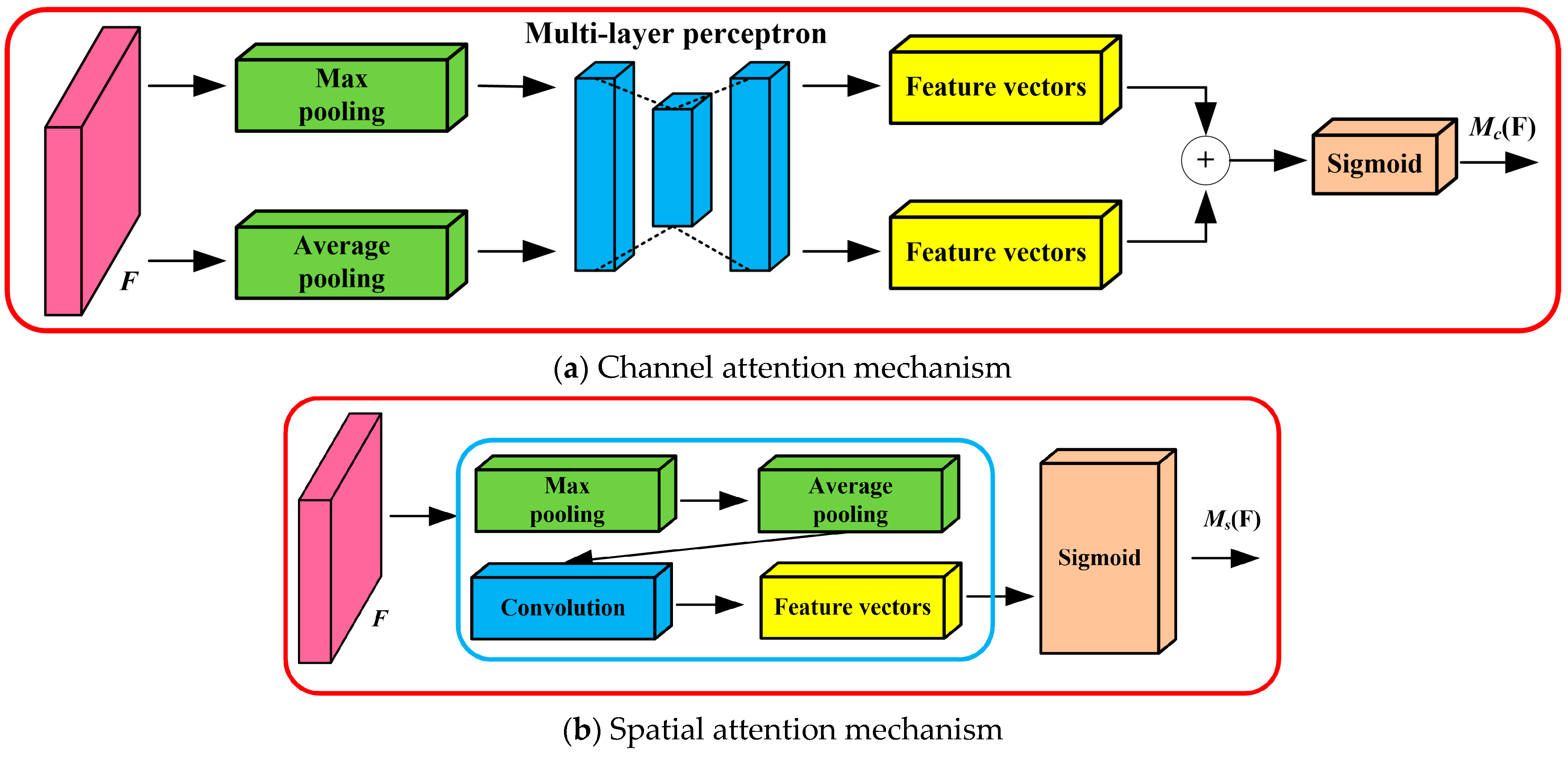
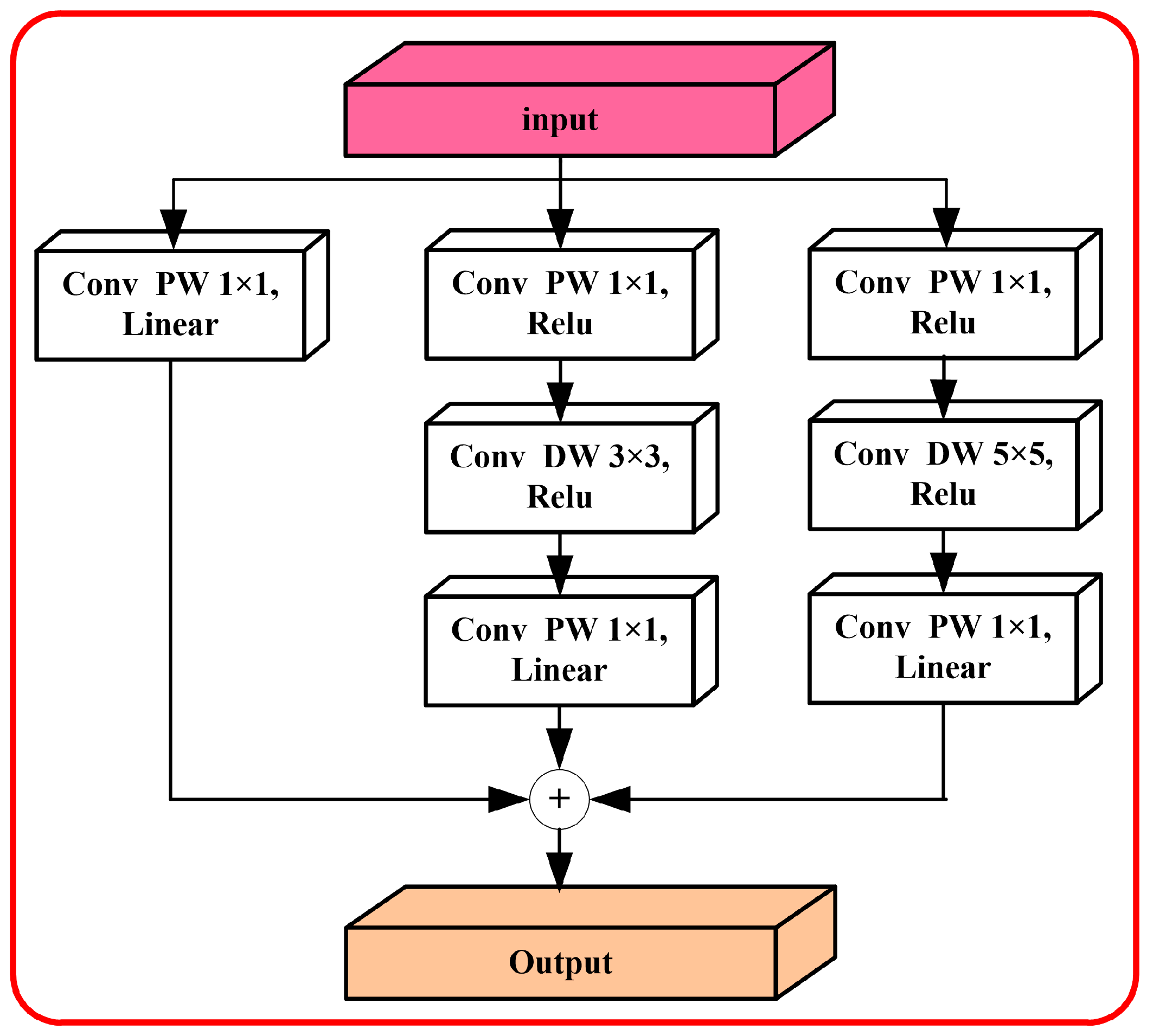
2.2. MobileNet Algorithm Based on Dual Attention

The main features of MobileNet V2 include: (1) the adoption of depth separable convolution in place of ordinary convolution to reduce model computation and parameter requirements; (2) the introduction of reverse residual structure to increase the number of network layers and enhance feature expressiveness; (3) replacement of nonlinear structures with linear Bottleneck structures to minimize the loss of low-dimensional feature information.
Based on the low power consumption characteristics of MobileNet V2 [37], MobileNet V2 has been selected as the main backbone network and improved through adjustments in width factor, attention module and multi-scale feature fusion. The network block diagram is shown in Figure 4.
The depth-separable convolution replaces the standard convolution with fewer parameters and computation [38]. The computation ratio of the depth-separable convolution with the standard convolution is given by:
H = D f 2 D k 2 M + D f 2 M N D f 2 D k 2 M N = 1 N + 1 D k 2
where Df represents the length of the input feature map and the number of channels, Dk is the length of depthwise convolution (DW) convolution kernel, and M is the number of pointwise convolution channels.
In feature extraction, the usual convolution kernel size is 3 × 3. The computation amount and parameter quantity of depth-separable convolution are approximately 1/9 of conventional convolution. MobileNet V2 incorporates the concept of ResNet and proposes the reverse residual structure. There are two typical methods: In the first method, PW convolution is used to increase the dimension, and DW convolution is used to extract the features from each channel, and PW convolution is then employed to reduce the feature dimensionality. When the step size is 1, a residual connection is established, while a series connection is established when the step size is 2; S The second method of the reverse residual structure first increases and then reduces dimensionality, which allows the network to accommodate smaller input and output dimensions, so as to reduce the computational load and parameters. At the same time, the residual connection can improve gradient propagation efficiency, with a deeper network layer.
An important parameter in the network is the width factor, which adjusts the number of convolution kernels in each module of the network to α times the original one, and the corresponding calculation load is:
T = α D f 2 D k 2 M + α 2 D f 2 M N
By adjusting α, the computational burden of the model is greatly reduced.
CBAM is an attention mechanism module that integrates channel and space [39]. It is embedded in a convolutional neural network for end-to-end training. The final channel attention is illustrated in Figure 5a.
M c F = σ W 1 W 0 F a v g + W 1 W 0 F m a x
where F is the input feature map, σ is the nonlinear activation function, Wi is the weight of layer i, and Favg and Fmax are the results of input F after the average pooling and kernel maximum pooling, respectively.
The spatial attention mechanism is shown in Figure 5b: the channel direction is averaged, and the kernel is maximally pooled to generate a feature description of size 2 × H × W, and the feature vector is obtained and activated by a convolution operation. The corresponding spatial attention mapping model is as follows:
M s F = σ ( f ( f c ( F a v g + F max ) ) )
where f is the convolution operation, and fc is the join operation. The complete calculation process of the CBAM module is
F A = M s F F F = M c F F
The CBAM module is integrated consecutively with the reverse residual block of MobileNet V2, which enables the module to focus on important features and suppress unnecessary ones in channel and spatial dimensions.
Inception uses multiple convolution checks of varying sizes to extract features from feature maps, which increases the adaptability of the network to different scales. The structure of Inception V1 is shown in Figure 6, which enriches features at spatial scales and proves beneficial for subsequent classification.
Given that the MobileNet V2 network uses depth-separable convolution, in order to give full play to the advantages of MobileNet and Inception, the Inception module step is set to 2 to remove the linear structure of residual short-form, as shown in Figure 7. Feature extraction is carried out through three parallel branches. Considering that stitching increases channel count in the output feature map, along with the total network parameters, an addition-based merging approach is chosen to reduce the overall model parameters.

3. Experimental Results and Analysis

3.1. Feature Extraction Algorithm

The result of leaf extraction is shown in Figure 8. To evaluate the algorithm performance, the following index [40] is introduced:
A O M = R s R g R s R g A V M = R s R g R s A U M = R g R s R g C M = 1 3 A O M + 1 A V M + 1 A U M
where the area overlap measure (AOM), the area over segmentation measure (AVM), the area under segmentation measure (AUM), and the combination measure (CM) are used to evaluate the algorithm’s performance. RS represents the result of manual leaf labeling and serves as the gold standard. Rg denotes the result of the algorithmic labeling. Values of AOM and CM are proportional to the segmentation results, while AVM and AUM values are inversely proportional to the segmentation results.
Typical tomato leaf diseases, as shown in Figure 9, were selected for the study. The results of the algorithm comparison are summarized in Table 2. The algorithm with a fixed threshold requires human-computer interaction for threshold selection, which exhibits low adaptability and presents different colors in the presence of the scab, resulting in the inability to accurately segment tomato leaves with a single threshold. On the other hand, OSTU [34] achieves threshold segmentation by calculating the gap between classes and setting the threshold, which is self-adaptive. However, due to the uniqueness of the threshold setting, the segmentation performance is somewhat limited. The GSO [41] algorithm searches for local optimal clustering, which realizes target recognition even under complex backgrounds, but it has some limitations in considering inter-class differences. The proposed algorithm fuses the OSTU algorithm with the attribute-weighted Bayes algorithm. This hybrid approach considers inter-class differences and intra-class similarities at a local level and exhibits a favorable effect on shadow suppression.
To show the effect of the algorithm, an analysis is conducted on the effect of Gabor filtering. As shown in Figure 10, a variety of conditions of leaves are observed: Figure 10a shows a smooth leaf surface; Figure 10b displays leaves damaged as a whole; Figure 10c illustrates leaves with a large number of spots on the surface; and Figure 10d exhibits leaves with yellowing surfaces. After Gabor filtering, Leaf 1 demonstrates rich texture features at low dimensions and angles, appearing relatively rich and smooth as dimensions and angles increase. Leaf 2 exhibits a robust response in high dimensions and angles, with high pixel values in the displayed image. Leaf 3 presents more textures after Gabor filtering. Overall, the response of Leaf 4 is not strong, but the lesion area exhibits a robust response in high dimensions and angles. Through the above analysis, the Gabor-filtered image is input into the depth learning module for disease classification.
To reflect the effect of feature extraction through Gabor filtering, the study takes the original image and Gabor-filtered image as input, uses a deep network for training, and compares their convergence performance, as shown in Figure 11. The results clearly demonstrate that the features extracted by Gabor are more representative, with the fast convergence speed of the algorithm, which brings it closer to the target function. This is because Gabor extracts multi-angle features, analyzes image characteristics, focuses on targets, and achieves efficient representation.

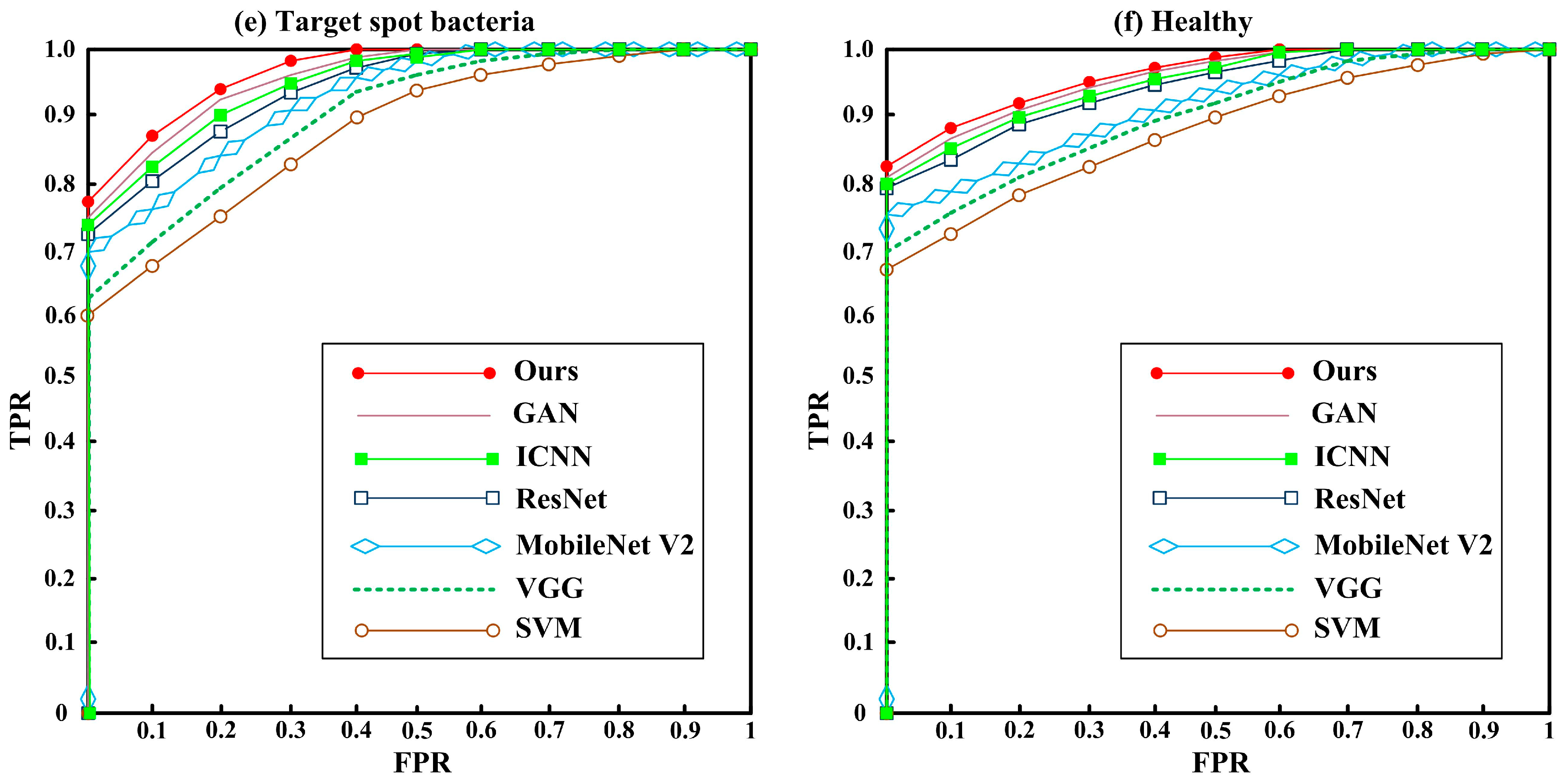
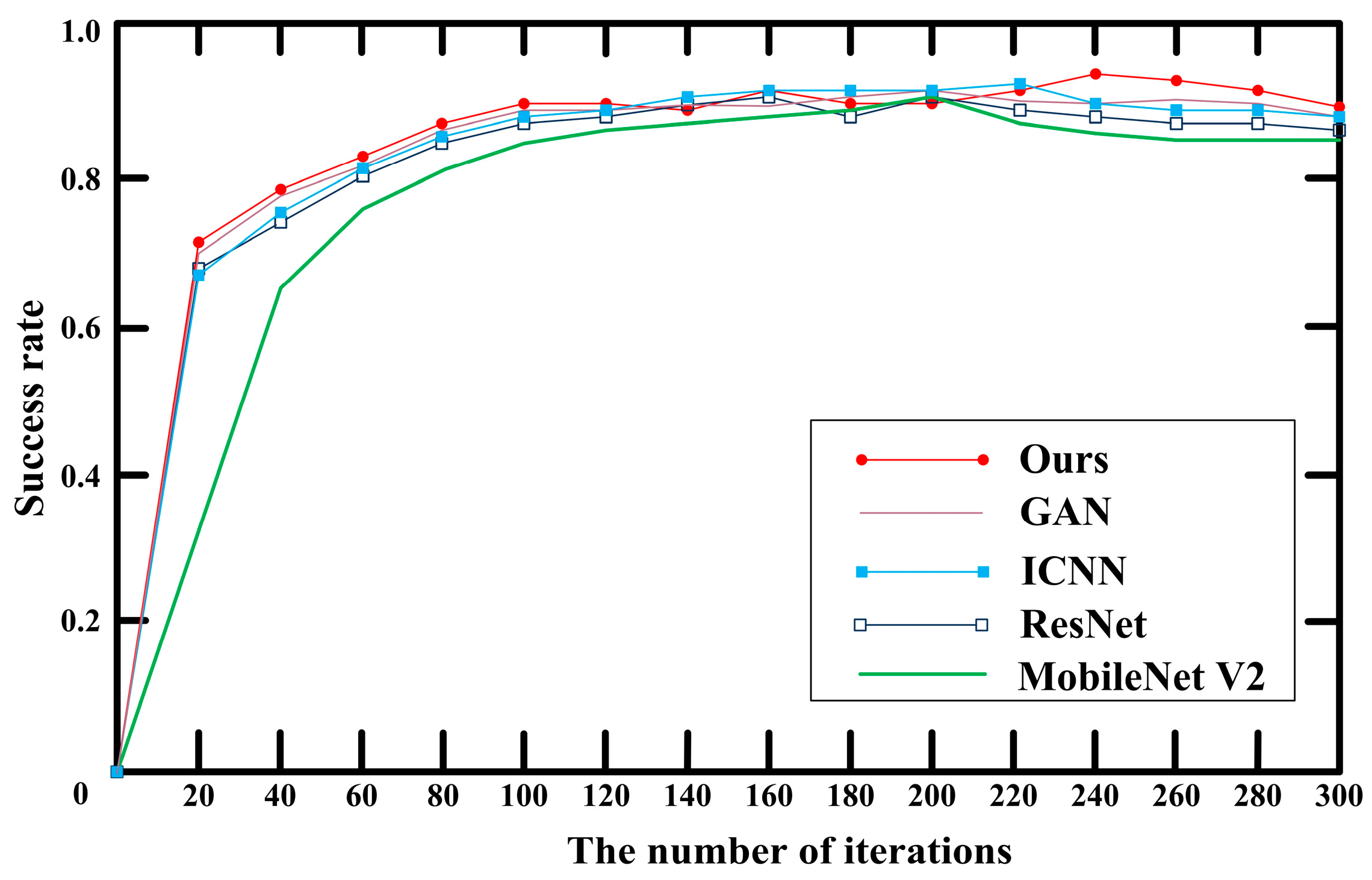
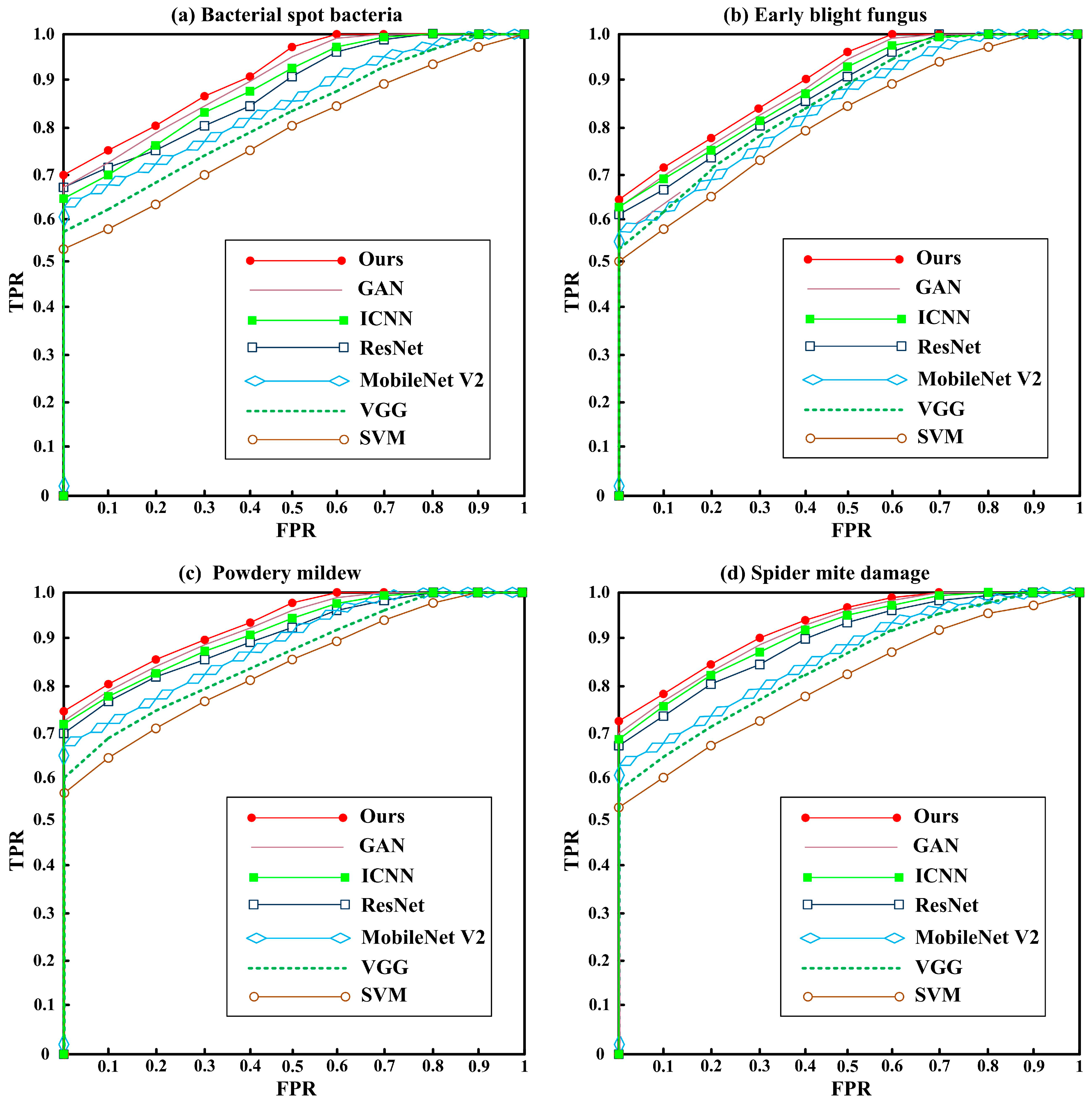
3.2. Comparison of Classification Algorithms

The following index are introduced for performance evaluation,
S E N = T P T P + F N S P E = T N T N + F P A C C = T P + T N T P + F P + T N + F N F P F = 1 A C C
where SEN reflects the detection performance for real objects. SPE reflects the detection performance for false objects. ACC reflects the ratio of correct test results to all samples in the test results, and FPF reflects the ratio of false test results diagnosed as true objects.
The comparison results of algorithms are shown in Table 3 and Table 4. It can be seen that the algorithm’s results without leaf area extraction are inferior to those with leaf area extraction, indicating that focusing on the area where leaves are located and reducing the influence of surrounding environments yields a positive effect. This verifies the good effect of the proposed leaf segmentation algorithm on subsequent disease clustering. The algorithm based on texture features proposed in Ref. [2] exhibits disease detection capabilities, albeit with slightly lower performance in terms of indicators. Ref. [23] conducts an in-depth analysis of the image characteristics and constructs a K-means model to improve the classification accuracy. Ref. [8] adds ANN based on an SVM classifier to introduce the classification task into multi-dimensional space, realize classification, and achieve certain results. Based on the current mainstream RESNET, Ref. [30] requires 50 iterations to achieve disease detection, but too many network parameters cause large consumption of computing resources. Ref. [37] constructs the traditional MobileNet V2 algorithm and refines the convolution calculation method to effectively boost the calculation speed and performance. Although SEN reaches an impressive 91%, this process is inconsistent with the human cognitive process. On the basis of MobileNet V2, the proposed algorithm adds an attention mechanism module in line with the process of human visual perception. The modification induces a further enhancement in algorithm performance, with superior results achieved.
Table 3 illustrates the limited effect of the traditional algorithm [2,8,23], but the algorithm based on depth network exhibits commendable performance. Therefore, deep learning algorithms [30,37,42,43] are compared, as shown in Figure 12. The ResNet algorithm [30] involves many parameters, resulting in slower convergence in the training process. In contrast, the MobileNet V2 algorithm [37] introduces a fast convolution change to reduce parameters, along with faster convergence. Improved CNN (ICNN) [42] based on color features focuses on the area where leaves are located and achieves satisfactory results. Generative adversarial networks (GAN) [43] further improve the effect by deeply mining intra-class and inter-class features in small sample situations.
On the basis of MobileNet V2, the proposed algorithm integrates the Inception module, which not only ensures swift convergence but also introduces visual attention, which is in line with the principle of human visual perception, alongside further improved performance.
Classified images of representative tomato diseases are selected: scab, early blight, powdery mildew, starred spider, spotted disease, and health to verify the performance of different algorithms, as shown in Figure 13. ResNet extracts local and global features for accurate image classification. MobileNet V2 demonstrates a certain classification performance in low-parametric network construction. VGG, through multi-layer filter convolution, can fully explore image features and realize classification. It can be seen from the figure that for single disease recognition, the accuracy of scab and early blight identification is low due to their striking similarity in spot shape, size and texture. As a result, misclassifications are more likely to occur in these cases. On the contrary, Health exhibits the highest accuracy. Based on MobileNet V2, the proposed algorithm adds the attention mechanism module to extract features across different scales, with superior results compared to other algorithms.

4. Conclusions

Plant diseases impose a serious impact on plant growth, making it of great significance to identify diseases through artificial intelligence. Since leaves are the direct manifestation of plant diseases, the research focuses on leaf features. To maximize the potential of traditional features and deep features, a comprehensive Plant Disease classification algorithm is proposed. (1) To solve the difficult classification of leaf diseases in complex backgrounds, the OSTU algorithm based on the Naive Bayes model is proposed to focus on the area where leaves are located and reduce background interference. (2) From the perspective of feature interpretability, a multi-dimensional feature model based on traditional features is constructed to fully explore leaf features. (3) From the perspective of deep learning, a MobileNet framework based on dual attention is established to achieve swift disease recognition. The algorithm underwent rigorous testing on the Plant Village open database, and the results showed that the algorithm could achieve plant disease classification.
Despite these achievements, there are also some problems in the research: The experimental dataset is limited and does not cover most diseases. Therefore, a larger dataset will be constructed to further integrate traditional features and deep features. Further studies will be conducted on interpretable fusion networks to promote research on plant disease prediction.

Author Contributions

Conceptualization, H.W. and S.Q.; methodology, H.Y. and X.L.; software, H.W. and S.Q.; validation, H.W.; formal analysis, All authors have read and agreed to the published version of the manuscript.

Funding

This work is supported by Light of West China (No. XAB2022YN10) and Shaanxi key research and development plan (No. 2018ZDXM-SF-093) and Shaanxi Province key industrial innovation chain (No. S2022-YF-ZDCXL-ZDLGY-0093 and 2023-ZDLGY-45).

Data Availability Statement

The data used to support the findings of this study are available from the corresponding author upon request.

Conflicts of Interest

The authors declare no conflict of interest.

References

  1. Al-Hiary, H.; Bani-Ahmad, S.; Reyalat, M.; Braik, M.; Alrahamneh, Z. Fast and accurate detection and classification of plant diseases. Int. J. Comput. Appl. 2011, 17, 31–38. [Google Scholar] [CrossRef]
  2. Kulkarni, A.H.; Patil, A. Applying image processing technique to detect plant diseases. Int. J. Mod. Eng. Res. 2012, 2, 3661–3664. [Google Scholar]
  3. Arivazhagan, S.; Shebiah, R.N.; Ananthi, S.; Varthini, S.V. Detection of unhealthy region of plant leaves and classification of plant leaf diseases using texture features. Agric. Eng. Int. CIGR J. 2013, 15, 211–217. [Google Scholar]
  4. Hossain, E.; Hossain, M.F.; Rahaman, M.A. A color and texture based approach for the detection and classification of plant leaf disease using KNN classifier. In Proceedings of the 2019 International Conference on Electrical, Computer and Communication Engineering (ECCE), Cox’s Bazar, Bangladesh, 7–9 February 2019; pp. 1–6. [Google Scholar]
  5. Singh, V.; Misra, A.K. Detection of plant leaf diseases using image segmentation and soft computing techniques. Inf. Process. Agric. 2017, 4, 41–49. [Google Scholar] [CrossRef]
  6. Kaur, R.; Singla, S. Classification of plant leaf diseases using gradient and texture feature. In Proceedings of the International Conference on Advances in Information Communication Technology & Computing, Thai Nguyen, Vietnam, 12–13 December 2016; pp. 1–7. [Google Scholar]
  7. Nanehkaran, Y.A.; Zhang, D.; Chen, J.; Tian, Y.; Al-Nabhan, N. Recognition of plant leaf diseases based on computer vision. J. Ambient. Intell. Humaniz. Comput. 2020, 11, 1–18. [Google Scholar] [CrossRef]
  8. Pujari, D.; Yakkundimath, R.; Byadgi, A.S. SVM and ANN based classification of plant diseases using feature reduction technique. IJIMAI 2016, 3, 6–14. [Google Scholar] [CrossRef]
  9. Brahimi, M.; Arsenovic, M.; Laraba, S.; Sladojevic, S.; Boukhalfa, K.; Moussaoui, A. Deep learning for plant diseases: Detection and saliency map visualization. In Human and Machine Learning; Springer: Cham, Switzerland, 2018; pp. 93–117. [Google Scholar]
  10. Mahmoud MA, B.; Guo, P.; Wang, K. Pseudoinverse learning autoencoder with DCGAN for plant diseases classification. Multimed. Tools Appl. 2020, 79, 26245–26263. [Google Scholar] [CrossRef]
  11. Sandesh Kumar, C.; Sharma, V.K.; Yadav, A.K.; Singh, A. Perception of plant diseases in color images through adaboost. In Innovations in Computational Intelligence and Computer Vision; Springer: Singapore, 2021; pp. 506–511. [Google Scholar]
  12. Hang, J.; Zhang, D.; Chen, P.; Zhang, J.; Wang, B. Classification of plant leaf diseases based on improved convolutional neural network. Sensors 2019, 19, 4161. [Google Scholar] [CrossRef]
  13. Atila, Ü.; Uçar, M.; Akyol, K.; Uçar, E. Plant leaf disease classification using EfficientNet deep learning model. Ecol. Inform. 2021, 61, 101182. [Google Scholar] [CrossRef]
  14. Sardogan, M.; Tuncer, A.; Ozen, Y. Plant leaf disease detection and classification based on CNN with LVQ algorithm. In Proceedings of the 2018 3rd International Conference on Computer Science and Engineering (UBMK), Sarajevo, Bosnia and Herzegovina, 20–23 September 2018; pp. 382–385. [Google Scholar]
  15. Deepa, N.R.; Nagarajan, N. Kuan noise filter with Hough transformation based reweighted linear program boost classification for plant leaf disease detection. J. Ambient. Intell. Humaniz. Comput. 2021, 12, 5979–5992. [Google Scholar] [CrossRef]
  16. Altan, G. Performance evaluation of capsule networks for classification of plant leaf diseases. Int. J. Appl. Math. Electron. Comput. 2020, 8, 57–63. [Google Scholar] [CrossRef]
  17. Pal, A.; Kumar, V. AgriDet: Plant leaf disease severity classification using agriculture detection framework. Eng. Appl. Artif. Intell. 2023, 119, 105754. [Google Scholar] [CrossRef]
  18. Liang, Q.; Xiang, S.; Hu, Y.; Coppola, G.; Zhang, D.; Sun, W. PD2SE-Net: Computer-assisted plant disease diagnosis and severity estimation network. Comput. Electron. Agric. 2019, 157, 518–529. [Google Scholar] [CrossRef]
  19. Yu, H.; Liu, J.; Chen, C.; Heidari, A.A.; Zhang, Q.; Chen, H.; Mafarja, M.; Turabieh, H. Corn leaf diseases diagnosis based on K-means clustering and deep learning. IEEE Access 2021, 9, 143824–143835. [Google Scholar] [CrossRef]
  20. Padol, P.B.; Yadav, A.A. SVM classifier based grape leaf disease detection. In Proceedings of the 2016 Conference on Advances in Signal Processing (CASP), Pune, India, 9–11 June 2016; pp. 175–179. [Google Scholar]
  21. Rani, F.P.; Kumar, S.N.; Fred, A.L.; Dyson, C.; Suresh, V.; Jeba, P.S. K-means clustering and SVM for plant leaf disease detection and classification. In Proceedings of the 2019 International Conference on Recent Advances in Energy-Efficient Computing and Communication (ICRAECC), Nagercoil, India, 7–20 March 2019; pp. 1–4. [Google Scholar]
  22. Trivedi, V.K.; Shukla, P.K.; Pandey, A. Automatic segmentation of plant leaves disease using min-max hue histogram and k-mean clustering. Multimed. Tools Appl. 2022, 81, 20201–20228. [Google Scholar] [CrossRef]
  23. Faithpraise, F.; Birch, P.; Young, R.; Obu, J.; Faithpraise, B.; Chatwin, C. Automatic plant pest detection and recognition using k-means clustering algorithm and correspondence filters. Int. J. Adv. Biotechnol. Res. 2013, 4, 189–199. [Google Scholar]
  24. Tamilselvi, P.; Kumar, K.A. Unsupervised machine learning for clustering the infected leaves based on the leaf-colours. In Proceedings of the 2017 Third International Conference on Science Technology Engineering & Management (ICONSTEM), Chennai, India, 23–24 March 2017; pp. 106–110. [Google Scholar]
  25. Hasan, R.I.; Yusuf, S.M.; Mohd Rahim, M.S.; Alzubaidi, L. Automatic clustering and classification of coffee leaf diseases based on an extended kernel density estimation approach. Plants 2023, 12, 1603. [Google Scholar] [CrossRef]
  26. Yadhav, S.Y.; Senthilkumar, T.; Jayanthy, S.; Kovilpillai, J.J.A. Plant disease detection and classification using cnn model with optimized activation function. In Proceedings of the 2020 International Conference on Electronics and Sustainable Communication Systems (ICESC), Coimbatore, India, 2–4 July 2020; pp. 564–569. [Google Scholar]
  27. Bhimavarapu, U. Prediction and classification of rice leaves using the improved PSO clustering and improved CNN. Multimed. Tools Appl. 2023, 82, 21701–21714. [Google Scholar] [CrossRef]
  28. Hatuwal, B.K.; Shakya, A.; Joshi, B. Plant leaf disease recognition using random Forest, KNN, SVM and CNN. Polibits 2020, 62, 13–19. [Google Scholar]
  29. Pareek, P.K.; Ramya, I.M.; Jagadeesh, B.N.; LeenaShruthi, H.M. Clustering based segmentation with 1D-CNN model for grape fruit disease detection. In Proceedings of the 2023 IEEE International Conference on Integrated Circuits and Communication Systems (ICICACS), Raichur, India, 24–25 February 2023; pp. 1–7. [Google Scholar]
  30. Mukti, I.Z.; Biswas, D. Transfer learning based plant diseases detection using ResNet50. In Proceedings of the 2019 4th International Conference on Electrical Information and Communication Technology (EICT), Khulna, Bangladesh, 20–22 December 2019; pp. 1–6. [Google Scholar]
  31. Li, M.; Cheng, S.; Cui, J.; Li, C.; Li, Z.; Zhou, C.; Lv, C. High-performance plant pest and disease detection based on model ensemble with inception module and cluster algorithm. Plants 2023, 12, 200. [Google Scholar] [CrossRef]
  32. Muammer, T.; Hanbay, D. Plant disease and pest detection using deep learning-based features. Turk. J. Electr. Eng. Comput. Sci. 2019, 27, 1636–1651. [Google Scholar]
  33. Ramesh, S.; Hebbar, R.; Niveditha, M.; Pooja, R.; Shashank, N.; Vinod, P.V. Plant disease detection using machine learning. In Proceedings of the 2018 International Conference on Design Innovations for 3Cs Compute Communicate Control (ICDI3C), Bangalore, India, 25–28 April 2018; pp. 41–45. [Google Scholar]
  34. Hoang, N.D. Detection of surface crack in building structures using image processing technique with an improved Otsu method for image thresholding. Adv. Civ. Eng. 2018, 2018, 3924120. [Google Scholar] [CrossRef]
  35. Vembandasamy, K.; Sasipriya, R.; Deepa, E. Heart diseases detection using Naive Bayes algorithm. Int. J. Innov. Sci. Eng. Technol. 2015, 2, 441–444. [Google Scholar]
  36. Yuan, Y.; Wang, L.N.; Zhong, G.; Gao, W.; Jiao, W.; Dong, J.; Shen, B.; Xia, D.; Xiang, W. Adaptive Gabor convolutional networks. Pattern Recognit. 2022, 124, 108495. [Google Scholar] [CrossRef]
  37. Srinivasu, P.N.; SivaSai, J.G.; Ijaz, M.F.; Bhoi, A.K.; Kim, W.; Kang, J.J. Classification of skin disease using deep learning neural networks with MobileNet V2 and LSTM. Sensors 2021, 21, 2852. [Google Scholar] [CrossRef]
  38. Dang, L.; Pang, P.; Lee, J. Depth-wise separable convolution neural network with residual connection for hyperspectral image classification. Remote Sens. 2020, 12, 3408. [Google Scholar] [CrossRef]
  39. Fu, H.; Song, G.; Wang, Y. Improved YOLOv4 marine target detection combined with CBAM. Symmetry 2021, 13, 623. [Google Scholar] [CrossRef]
  40. Qiu, S.; Jin, Y.; Feng, S.; Zhou, T.; Li, Y. Dwarfism computer-aided diagnosis algorithm based on multimodal pyradiomics. Inf. Fusion 2022, 80, 137–145. [Google Scholar] [CrossRef]
  41. Selvanambi, R.; Natarajan, J.; Karuppiah, M.; Islam, S.H.; Hassan, M.M.; Fortino, G. Lung cancer prediction using higher-order recurrent neural network based on glowworm swarm optimization. Neural Comput. Appl. 2020, 32, 4373–4386. [Google Scholar] [CrossRef]
  42. Kaya, Y.; Gürsoy, E. A novel multi-head CNN design to identify plant diseases using the fusion of RGB images. Ecol. Inform. 2023, 75, 101998. [Google Scholar] [CrossRef]
  43. Lamba, S.; Saini, P.; Kaur, J.; Kukreja, V. Optimized classification model for plant diseases using generative adversarial networks. Innov. Syst. Softw. Eng. 2023, 19, 103–115. [Google Scholar] [CrossRef]
Figure 1. Experiment database.
Algorithms 16 00442 g001
Figure 2. Algorithm flow chart.
Algorithms 16 00442 g002
Figure 3. OSTU algorithm based on naive Bayes model.
Algorithms 16 00442 g003
Figure 4. Attention-based MobileNet framework.
Algorithms 16 00442 g004
Figure 5. Attention mechanism module.
Algorithms 16 00442 g005
Figure 6. Inception V1 module.
Algorithms 16 00442 g006
Figure 7. Scale feature fusion module.
Algorithms 16 00442 g007
Figure 8. The effect of our object extraction.
Algorithms 16 00442 g008
Figure 9. Typical tomato diseases.
Algorithms 16 00442 g009
Figure 10. The effect of Gabor filtering.
Algorithms 16 00442 g010
Figure 11. Iteration curve.
Algorithms 16 00442 g011
Figure 12. Algorithm success rate curve.
Algorithms 16 00442 g012
Figure 13. ROC curve.
Algorithms 16 00442 g013aAlgorithms 16 00442 g013b
Table 1. Data classification.
AppleHealthySreawberryHealthy
ScabGeneralScorchGeneral
SeriousSerious
Cedar RustGeneralTomatoBacterial Spot BacteriaGeneral
SeriousSerious
CherryHealthyEarly Blight FungusGeneral
Powdery MildewGeneralSerious
SeriousLate Blight Water MoldGeneral
CornHealthySerious
Cercospora Zeaemaydis Techon and DanielsGeneralLeaf Mold FungusGeneral
SeriousSerious
Puccinia PolvsoraGeneralTarget Spot BacteriaGeneral
SeriousSerious
Corn Curvularia Leaf Spot FungusGeneralSeptoria Leaf Spot FungusGeneral
SeriousSerious
Maize dwarf mosaic virusSpider Mite DamageGeneral
GrapeHealthySerious
Black Rot FungusGeneralYLCV VirusGeneral
SeriousSerious
Black Measles FungusGeneralTomv
SeriousPepperHealthy
Leaf Blight FungusGeneralScabGeneral
SeriousSerious
CitrusHealthyPotatoHealthy
Greening JuneGeneralEarly Blight FungusGeneral
SeriousSerious
PeachHealthyLate Blight FungusGeneral
Bacterial SpotGeneralSerious
SeriousPepperScabGeneral
PepperHealthySerious
Table 2. (1) The algorithm extracts the performance of tomato leaves with bacterial spot bacteria. (2) The algorithm extracts the performance of tomato leaves with early blight fungus. (3) The algorithm extracts the performance of tomato leaves with powdery mildew. (4) The algorithm extracts the performance of tomato leaves with spider mite damage. (5) The algorithm extracts the performance of tomato leaves with target spot bacteria. (6) The algorithm extracts the performance of healthy tomato leaves.
(1)
AlgorithmAOMAVMAUMCM
T0.710.410.340.65
OSTU [34]0.760.350.330.70
GSO [41]0.820.340.310.72
Ours0.850.310.290.75
(2)
AlgorithmAOMAVMAUMCM
T0.740.330.350.69
OSTU [34]0.810.310.320.73
GSO [41]0.850.270.290.76
Ours0.870.260.270.78
(3)
AlgorithmAOMAVMAUMCM
T0.750.310.330.70
OSTU [34]0.780.270.310.73
GSO [41]0.840.240.280.77
Ours0.880.230.240.80
(4)
AlgorithmAOMAVMAUMCM
T0.740.340.270.71
OSTU [34]0.810.350.250.74
GSO [41]0.860.240.220.8
Ours0.910.210.190.84
(5)
AlgorithmAOMAVMAUMCM
T0.790.310.250.74
OSTU [34]0.870.280.230.79
GSO [41]0.910.230.190.83
Ours0.930.180.170.86
(6)
AlgorithmAOMAVMAUMCM
T0.860.260.230.79
OSTU [34]0.890.230.220.81
GSO [41]0.920.170.180.86
Ours0.950.150.160.88
Table 3. Algorithm results without leaf region extraction.
AlgorithmSENSPEACCFPF
Texture [2]0.650.310.720.28
K-means [32]0.720.290.760.24
SVM + ANN [8]0.750.250.800.20
ResNet [30]0.810.200.820.18
MobileNet V2 [37]0.840.180.840.16
ICNN [42]0.850.150.860.14
GAN [43]0.860.120.890.11
Ours0.860.100.910.09
Table 4. Algorithm results with leaf region extraction.
AlgorithmSENSPEACCFPF
Texture [2]0.710.260.790.21
K-means [32]0.790.240.850.15
SVM + ANN [8]0.810.210.870.13
ResNet [30]0.850.150.910.09
MobileNet V2 [37]0.910.130.960.04
ICNN [42]0.910.110.970.03
GAN [43]0.920.100.960.04
Ours0.940.080.980.02
Disclaimer/Publisher’s Note: The statements, opinions and data contained in all publications are solely those of the individual author(s) and contributor(s) and not of MDPI and/or the editor(s). MDPI and/or the editor(s) disclaim responsibility for any injury to people or property resulting from any ideas, methods, instructions or products referred to in the content.

