Learning from Imbalanced Datasets: The Bike-Sharing Inventory Problem Using Sparse Information ^†

Abstract

In bike-sharing systems, the inventory level is defined as the daily number of bicycles required to optimally meet the demand. Estimating these values is a major challenge for bike-sharing operators, as biased inventory levels lead to a reduced quality of service at best and a loss of customers and system failure at worst. This paper focuses on using machine learning (ML) classifiers, most notably random forest and gradient tree boosting, for estimating the inventory level from available features including historical data. However, while similar approaches adopted in the context of bike sharing assume the data to be well-balanced, this assumption is not met in the case of the inventory problem. Indeed, as the demand for bike sharing is sparse, datasets become biased toward low demand values, and systematic errors emerge. Thus, we propose to include a new iterative resampling procedure in the classification problem to deal with imbalanced datasets. The proposed model, tested on the real-world data of the Citi Bike operator in New York, allows to (i) provide upper-bound and lower-bound values for the bike-sharing inventory problem, accurately predicting both predominant and rare demand values; (ii) capture the main features that characterize the different demand classes; and (iii) work in a day-to-day framework. Finally, successful bike-sharing systems grow rapidly, opening new stations every year. In addition to changes in the mobility demand, an additional problem is that we cannot use historical information to predict inventory levels for new stations. Therefore, we test the capability of our model to predict inventory levels when historical data is not available, with a specific focus on stations that were not available for training.

1. Introduction

Bike-sharing systems are one of the most popular and environmentally friendly forms of shared mobility. Traditional sharing systems allow the pickup and drop-off of bikes at fixed stations (or throughout an operational area if the system is free-floating) and have proven to be an effective solution for first-/last-mile mobility [1].

To keep a high quality of service, bike-sharing operators face two major problems, namely, the optimal inventory problem and the rebalancing problem [2]. The fact that bike-sharing users can take a bicycle from and return it to any station in the system leads to an imbalanced state, in which some stations are full while others stay empty. This nonhomogeneous distribution of bicycles lowers the overall level of service of the system [3]. The rebalancing problem consists in reorganizing the fleet location in time and space to re-establish the optimal level of service [4], an operation that can be performed when the system is shut down or the demand is low (static rebalancing) or while it is running (dynamic rebalancing) [1,5]. To reduce operational costs generated by rebalancing operations, it is fundamental to know the correct number of bicycles (and available docks if the service is station-based) required to achieve the optimal level of service, i.e., the target inventory values for the rebalancing procedure. This problem is known as the optimal inventory problem [6], and since inventory levels depend on user behavior [7], it is extremely challenging. While many rebalancing studies assume that the target inventory level for each station is known, to the best of the authors’ knowledge, only a few studies have focused on combining rebalancing with target-level computation.

This paper tests specific machine learning (ML) techniques that estimate the inventory level required to address the station-based bike-sharing static rebalancing problem. Specifically, the use of decision tree classifiers—most notably a random forest classifier (RFC) and gradient tree-boosting classifier (GTBC)—is investigated. Due to the vast amount of data publicly available, decision trees have already been used to study bike-sharing systems [8,9]. However, the majority of machine learning models adopted in the literature (e.g., decision trees but also neural networks and support vector machines) assume the data to be well-balanced. This assumption is not met in the case of the inventory problem [10]. Therefore, in this paper, we propose an ad hoc iterative resampling procedure that allows to accurately predict inventory levels using several features, including historical data, in the case of imbalanced datasets. The main contributions of this paper are summarized below:

• The inventory problem is formulated as a classification problem that can be easily solved using decision trees (or any other state-of-the-art classifier);
• While traditional classifiers over-represent the majority class, this paper presents a novel resampling technique that better leverages data and provides better estimates for rare observations;
• The proposed algorithm can be used to compute both an upper-bound and a lower-bound value for the bike-sharing inventory problem, thus yielding to different possible configurations;
• Although mainly based on historical data, the proposed approach can also be used to solve the inventory problem for new stations, for which historical information is not available;
• The proposed model is easily implementable into an ITS-based decision support system for also supporting bike-sharing companies in a day-to-day framework, thus helping in improving operations.

Points 4 and 5, i.e., predictions for new stations and the proposal of a rolling horizon approach to make day-to-day forecasts, are completely new developments with respect to the previous presentation of this work [10].

The method has been applied and validated using the data of the New York City Bike service.

The remainder of the paper is organized as follows: Section 2 introduces the relevant literature, namely, the existing research on inventory and rebalancing problems, but also provides a short overview of the most popular solutions to deal with imbalanced datasets in ML. As a consequence, the main gaps of the literature are identified, and possible solutions are discussed. The methodology is reported in Section 3: specifically, (i) how the target values of the inventory problem used as the benchmark in the paper are computed; (ii) the inventory problem formulation using ML classifiers to make previsions (for both existing and new stations); and (iii) the proposed iterative resampling technique to deal with data imbalance. The application and related results are reported in Section 4, followed by the conclusion.

2. Related Research

2.1. The Inventory Problem and the Rebalancing Problem

Developing an inventory model for a traditional station-based bike-sharing service is particularly challenging as it needs to capture two features: (1) the demand for bicycles; (2) the demand for docks—i.e., finding an empty dock where the user can return the rental bicycle [11]. Therefore, to simply find the number of bicycles that serves the demand is not sufficient [7].

The uneven distribution of vehicles and docks in the system causes some stations to be empty (or entirely full), creating shortages of both bicycles and docks. To prevent this shortage, several studies introduced rebalancing techniques that aim at evenly redistribute bicycles and docks in the system [12]. Traditionally, the problem is solved using either optimization techniques [12] or ML models [8]. Optimization techniques translate the problem into a mathematical language and focus on tractability and convergence properties. The most common approach is to formulate the problem as a one-commodity pickup-and-delivery capacitated vehicle-routing problem, which is then solved using mixed-integer linear programming [12]. This approach has also been extended to other station-based shared mobility services, such as car sharing [13]. The complexity of the algorithm depends on whether the objective is to achieve a complete rebalancing (all stations are jointly optimized) or a partial one (only a subset of stations is optimized), with the former case being far more complex than the latter [14]. Traditional algorithms for solving the problem include tabu search [15] and branch-and-cut [16]. However, as exact formulations are not suited for real-life instances, heuristic models have been developed to solve the problem in practice [9,17].

In recent years, other authors have proposed using ML instead of optimization techniques to solve the rebalancing problem. The most popular models include decision trees [8,9], neural networks [18], deep neural networks [19,20], and clustering techniques [2]. The main convenience of these models is that they are suited for large-scale, real-life applications and require limited assumptions of user behavior.

The models discussed up to this point also present several differences in the operational approach. For instance, [15] provides a price mechanism to support rebalancing, while [9] assumes that rebalancing operations are performed by the sharing company; these approaches are translated into different parameters and objective functions. However, most repositioning studies, including those using ML, assume that the inventory level (i.e., the optimal number of docks/bicycles at any given time) is known from historical data or by using an existing demand model [7]. To date, only a few studies have focused on how to compute the optimal target levels while considering the rebalancing problem.

Among the studies that have focused on the inventory levels, [21] proposed a mixed-integer program formulation to find the inventory levels that minimize the cost of rebalancing. Alternatively, [22] formulated the inventory problem as a nonstationary Markov chain model that computes the most likely optimal inventory levels during the day. Ref. [23] identifies an upper bound and a lower bound for the inventory level using historical information. A similar approach is used in [24]. Ref. [7] also identifies an upper bound and a lower bound for the inventory level using mixed-integer optimization. One of the main limits of the previous approaches, however, is that the model explicitly minimizes the journey dissatisfaction levels with respect to the user and cannot be used if the operator has different goals (such as maximizing profit).

Another aspect to highlight is the role of IT technologies. While bike-sharing systems date back to 1960, this service was initially unsuccessful due to several issues, e.g., vandalism and theft [25] The IT revolution not only enabled operators to develop a better service but also to improve aspects related to strategic and operational planning [26]. Thanks to the large amount of historical data, often openly available, it is now possible to optimize not only the fleet size and location of docks but also the entire supply chain of the system, from ordering vehicles and spare parts to scheduling fleet maintenance [27]. This is expected to become a primary problem in the future. Systems where the demand exceeds the capacity may not require rebalancing. In addition, to investigate a potential unserved demand, operators will therefore focus on optimizing inventory levels while also considering the scheduled maintenance, hence reducing costs and increasing margins [28].

2.2. Learning from Imbalanced Datasets

Data Imbalance means that an uneven distribution of classes exists within the data, and it is a serious threat for classification problems, as standard classifiers assume the data to be well-balanced. In general, class imbalance is one of the greatest challenges in machine learning and data mining research [29] and can appear in two main forms: rare classes or rare cases [30]. The problem of rare classes refers to datasets that contain different proportions of observations (or instances) per class. The concept of rare cases refers instead to the sparse distribution of examples in the feature space [30]. The two problems are closely related, as they both result in an uneven distribution of observations. However, rare cases refer to data that is sparse by nature, while a rare class might simply depend on the sampling procedure.

Different approaches have been proposed in the literature to deal with imbalanced datasets, and they can be broadly divided into two: methods working at a learner level and methods working at a sampling level [31]. Methods working at a learner level modify an existing algorithm to increase the precision of the minority class. The most common approach is to use cost-sensitive approaches, in which the learner associates the rare class with some weights to compensate for data imbalance [32]. The main limitation of these methods is that they are designed for specific learners and are hard to generalize. Methods working at a sampling level are considered more general [33] as they use resampling to artificially rebalance the dataset. Over-sampling and under-sampling are the most common resampling techniques [34]; this approach consists in creating a balanced dataset by artificially generating new observations for the rare class. In the case of over-sampling, the algorithm creates new artificial data points for the minority class. The SMOTE (synthetic minority over-sampling technique) approach is one of the most common techniques [35]. The other main option is to use under-sampling procedures, which consists of using a subsample of the majority class [36]. One particularly advanced model is balance cascading [37]: in this algorithm, the model iteratively drops observations from the majority class that are correctly classified. The argument is that these observations are redundant and might negatively affect the quality of the classifier, making it biased toward the majority class.

2.3. Discussion

In this paper, we propose a novel model that uses ML—most notably decision trees—to address the inventory problem as a classification problem. The main argument for this decision is that inventory levels are usually estimated from historical data, and ML captures historical trends better than simple averages. Similar to other approaches presented in the literature, our model will compute upper bounds and lower bounds for the inventory level. Moreover, as it is based on data, it is not limited to one specific goal, as it usually happens when using optimization.

As previously reported, the main problem in using ML for solving the inventory problem is data imbalance. In the case of the inventory problem, we deal with both rare cases and rare classes. Though existing algorithms for data imbalance demonstrate promising advantages, they also have several disadvantages, most notably over-generalization [38]. Simply stated, dock stations characterized by a high demand strongly differ from those characterized by a low demand. No model will be able to properly predict both, which means that the model will either provide poor predictions or fit the dominant class. Case-specific algorithms, tailor-made to the problem, can address the over-generalization issue [39]. Decision trees are among the most interpretable ML classifiers as they allow to understand how each feature contributes to the classification effort. Differently from standard decision trees, random forest classifiers (RFCs) and gradient tree-boosting classifiers (GTBCs) combine multiple models to make predictions, which allow them to provide better output. Inspired by these models, we proposed an iterative resampling algorithm that leverages multiple learners. Similar to balance cascading, at each iteration the model drops those observations that belong to the majority class and are properly classified. However, instead of simply dropping some observations and repeating the training exercise on the new dataset, the proposed model drops the majority class entirely and defines a new classification problem. Therefore, the model outputs an ensemble of models, each of them having different classes, different features, and different prediction capabilities. The final prediction is a combination of all these classifiers and provides more reliable predictions compared to using a single learner.

3. Methodology

The system considered is station-based with rebalancing activity conducted during the night (i.e., low demand, static rebalancing).

The proposed method to approach the inventory problem as a ML classification problem is here described. It will be adopted for both defining the target demand levels for each station and estimating the demand for new stations. The results of our proposed method will be compared with the results of common approaches based on historical data (benchmark values, as described in the following section). Finally, the resampling technique used to avoid data imbalance is presented.

3.1. Benchmark Values from Historical Data

The benchmark values from historical data are computed in terms of a set of options, from a lower bound (LB) to an upper bound (UB), never producing a lake of bikes or docks [7,22,23,24]. To compute the LB and UB, once departures and arrivals in a bike-sharing station are collected (Figure 1), the cumulative curves for departures and arrivals can be derived, as well as the cumulative net curve, i.e., the difference between arrivals and departures (Figure 2).

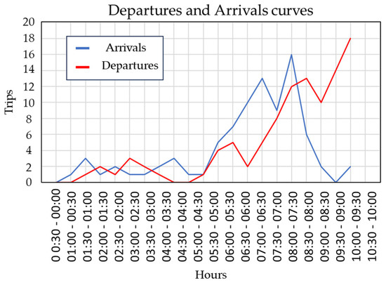
Figure 1. Hypothetical trend of bike departures and arrivals (Source: own elaboration).

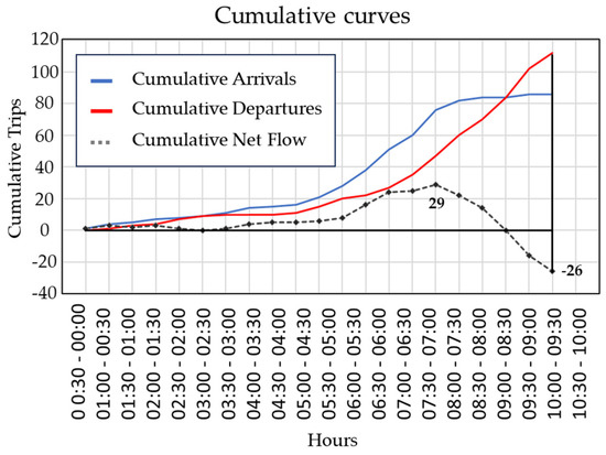
Figure 2. Hypothetical cumulative net flow (Source: own elaboration).

Considering the cumulative net curve, its highest value is the minimum number of docks required to respond to the arrival demand at the station (or the dock’s lower bound—LB). Instead, its lowest value is the minimum number of bikes required to respond to the demand (bikes’ LB). The upper bound (UB), for docks and bikes, can be computed as the difference between the capacity C of the station and, respectively, the LB for bikes and docks [10], as in the following equations:

$${LB}_{dock}=\mathrm{m}\mathrm{a}\mathrm{x}\left(Cumulativenetflow\right)$$

(1)

$${LB}_{bikes}\left\{\begin{array}{c}min\left|Cumulativenetflow\right| ifCumulativenetflow<0\\ {LB}_{bikes}=0ifCumulativenetflow\ge 0\end{array}\right.$$

(2)

$${UB}_{bike}=\mathrm{C}-{LB}_{dock}$$

(3)

$${UB}_{dock}=\mathrm{C}-{LB}_{bikes}$$

(4)

3.2. The Inventory Problem as a Classification Problem Using Machine Learning

An ML classifier is an algorithm that returns the probability $p(Y=k)$ that the dependent variable Y belongs to a certain class k. Without the loss of generality, in the case of a supervised classifier, we can write

$$p\left(Y=k\right)=\mathcal{H}(\mathit{X},\mathsf{\Theta })$$

(5)

where $\mathcal{H}$ is a general nonlinear-model, X is the set of features (or independent variables) used to predict the probability $p\left(Y=k\right)$, and $\mathsf{\Theta }$ is a set of hyperparameters. The form of the model $\mathcal{H}$ depends on the type of classifier used (neural networks, decision trees, etc.) and the hyperparameters $\mathsf{\Theta }$, which explain the relationship between dependent and independent variables. To obtain the correct value of $\mathsf{\Theta }$, supervised models use a training set (i.e., a dataset where both dependent and independent variables are known) and compute the set of parameters $\mathsf{\Theta }$ that, given the training set, is more likely to reproduce the data. In the case of decision trees, Equation (5) can be rewritten as follows:

$$p\left(Y=k\right)=DT(\mathit{X},\mathit{\theta },\mathsf{\Theta })$$

(6)

where $\mathit{\theta }$ is the set of hyperparameters/weights that is associated with the feature vectors X. Similar to linear regression or logistic regression, $\mathit{\theta }$ represents the impact that each feature has on the prediction. This aspect related to interpretability makes decision trees among the simplest and most interpretable classifiers.

In order to use Equations (5) and (6) in the context of the inventory problem, it is necessary to define the dependent and independent variables. In the case of the dependent variables, our objective is to estimate the UB and LB of the demand for bikes/docks; therefore, we might want to set $Y^{UB}=UB$ and $Y^{LB}=LB$ in Equations (5) and (6). The problem is that classification problems require discrete variables while the LB/UB for bikes/docks are continuous ones. Therefore, we need to define classes for the UB and LB and transform $Y^{UB}/Y^{LB}$ into categorical variables. To do so, we introduce the error term $\epsilon$, which represents the expected precision of the model. Given $\epsilon$, we can say that a certain value of the UB belongs to the class $k$ if, and only if,

$$\left\{\begin{array}{ll}UB\in k& if{UB}^k-\epsilon <UB\le {UB}^k+\epsilon \hspace{1em}with{UB}^k-\epsilon \ge 0\\ UB\notin k& otherwise\end{array}\right.$$

(7)

where ${UB}^k$ is the center of the class. To provide a numerical example, the first class will have a center equal to zero, therefore ${UB}^0=0$. Assuming an error term $\epsilon$ of 2 bikes, all target values $UB\le 2$ will belong to Class 0. The second class will assume ${UB}^1=4$, therefore all observations $2<UB\le 6$ will belong to this class, and so on. Note that for $\epsilon =0.5$, each integer represents a separate class. The same procedure applies for the LB.

Creating independent variables is straightforward, as any feature can potentially be used within the ML classifier. In general, we argue that three features should be used in the context of the inventory problem:

$$\mathbf{X}=\left\{{\mathbf{X}}_{behavioral},{\mathbf{X}}_{endogenous},{\mathbf{X}}_{exogenous}\right\}$$

(8)

The difference between endogenous and exogenous features is straightforward. Endogenous features are explained by other variables within the model (for instance, lagged variables such as the departures and arrivals collected in the station the day before), while exogenous variables are not explained by other variables within a model (e.g., location of the station).

The distinction between these two variables is not important when we want to predict the target values for an existing station, but it becomes relevant when the objective is to predict the demand for a new station, for which exogenous features might not be available. Finally, as the target levels depend on user behavior [7], some features that approximate user behavior will also help the model provide better estimates.

In this research, we have no access to behavioral features such as the value of time or individual preferences. Therefore, we use weather data to approximate ${\mathbf{X}}_{behavioral}$. The reason is that, in the case of bike sharing, it has been observed that user behavior is highly correlated to weather data, which allows to partially compensate for the lack of behavioral features [40].

To propose a formulation that can be deployed in practice, the classification problem proposed in Equation (6) can be rewritten as a time series and be used to make day-to-day predictions:

$$p\left(Y^d=k\right)=DT({\mathbf{X}}^{d-1},{\mathbf{X}}^{d-2},\dots ,{\mathbf{X}}^{d-T},\mathit{\beta },\mathsf{\Theta })$$

(9)

where ${\mathbf{X}}^d$ is the set of features for a given day, T represents the time lag, i.e., how many past days are used to predict the demand for the next day, and $Y^d$ is the prediction for day d. With respect to Equation (6), we have a new dataset every day, and the procedure must be repeated daily.

3.3. Iterative Resampling and Data Imbalance

Though traditional techniques for data imbalance provide many benefits, in the case of the inventory problem, off-the-shelf techniques might over-generalize the problem. Simply stated, they might identify a set of hyperparameters $\mathsf{\Theta }$ that is too general, as they assume that the same features that are important for the majority class are also important for the minority class. Therefore, this section introduces a resampling technique that generates and estimates, in an iterative manner, balanced data classes. The model focuses on a database-splitting function, and it is intuitively illustrated in Figure 3.

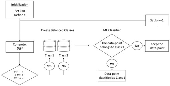
Figure 3. Illustrative example of the resampling technique (Source: own elaboration).

Starting from the entire dataset, the approach divides the data into 2 classes. Class 1 corresponds to $k=0$, therefore ${UB}^0=0$. All the other data points are inserted in Class 2. The objective is to create two balanced classes of data. In Figure 3, we assume that two classes are sufficient. In practice, additional classes are created until all classes are the same size. However, only Class 1 is computed using the system of Equation (6), therefore ${UB}^k$ and $\epsilon$, while all other classes are computed to ensure balance within the data, i.e., the only criterion to create all other classes is that they must have the same number of data points. At each iteration, a decision tree classifier is used to classify the data. All data points that are classified as Class 1 are considered properly classified. All remaining observations are included in a new dataset. At this point, we set $k=k+1$, and we repeat the operation on the new reduced dataset. The operation continues until all data points have been classified. As Figure 3 is a purposely trivial example, the procedure is depicted in Algorithms 1 and 2, where E is the tolerance error for the class imbalance, i.e., how much class imbalance is allowed in the system.

Algorithm 1: Iterative Resampling Technique

Procedure: resampling (X, Y, ε, k, E) ForUB in Y         ${UB}^k={UB}^{k-1}+2\epsilon$ if ${UB}^k-\epsilon <UB\le {UB}^k+\epsilon$        $UB\in {Class}^1$ Else $UB\in {Class}^2$ $\mathrm{Set}\mathrm{Len}=\mathrm{length}\left({Class}^2\right)$ If $\mathrm{length}\left({Class}^1\right)<\mathrm{Len}+E$  Set n = $\mathrm{Len}/\mathrm{length}\left({Class}^1\right)$ Split ${Class}^2$ in n classes If $\mathrm{length}\left({Class}^1\right)>\mathrm{Len}-E$ Set n = $\mathrm{length}({Class}^1$)/Len Split ${Class}^1$ in n classes Return (X, Class)

Algorithm 2: Iterative ML Classifier

$\mathbf{Procedure}:\hspace{1em}\mathcal{H}IT(\mathbf{X},\mathbf{Y},\mathsf{\Theta })$ Set $\epsilon$, k, E Set k = 0 While  $(\mathbf{X},\mathbf{Y})$ is not empty: $\mathbf{ClassLabel}=\mathrm{resampling}(\mathrm{X},\mathrm{Y},\epsilon$, k, E) $\mathrm{Train}\mathrm{ML}\mathrm{Classifier}\hspace{1em}DT\left(\mathit{X},\mathit{\beta },\mathsf{\Theta }\right)$ For $\mathrm{X},\mathrm{Y}\mathrm{i}\mathrm{n}{Class}^1$: $\mathrm{remove}\mathrm{X},\mathrm{Y}\mathrm{from}\mathbf{X},\mathbf{Y}$        Set k = k + 1

It should be noted that, as the lower and upper bounds are computed using the cumulative net flow and not the demand, stations with different demand levels (e.g., in the city center or in the suburbs) may still have similar inventory levels and therefore be grouped in the same class. This could create issues during the classification, as these stations may exhibit a different behavior. Therefore, the model should ideally incorporate endogenous features, as previously mentioned, to account for this phenomenon.

The resampling function needs to be used together with the learner in an iterative manner. This is illustrated in Algorithm 2. Specifically, the function determines a balanced group of classes to be forecasted at each iteration. Once a maximum number of classes is defined for each prediction group, the function generates the set of classes that have to be predicted (A) and the set to predict later (B). At each iteration, the machine learning classifier is adopted to forecast (A), and the process goes ahead on the group (B). The procedure is repeated until all points have been properly predicted. An illustrative example is presented in Figure 4.

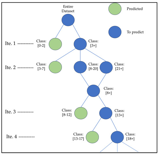
Figure 4. Example of the iterative procedure (Source: own elaboration).

The proposed resampling procedure can be considered as a hybrid model, as it works both at a learner level and at the sampling level. Specifically, at each iteration, a different model is trained. For instance, the models used in Figure 4 to predict Class (0–2) and Class (3–7) are different. At the same time, any classifier can be used, as the model leverages different training sets at each iteration and does not modify the learner. Similarly, it should be noted that the iterative resampling procedure is used on the training set, as it requires knowledge of both dependent and independent variables.

4. Numerical Results

4.1. Case Study

The methods discussed in the previous section are now tested adopting real data from the Citi Bike station-based service in New York City, US (about 900 stations and 14,500 shared bikes available). In particular, the database for the machine learning derives from over 17 million rides during 2018.

The trained models estimate the LB/UB of bikes adopting the available features reported in Table 1. Given the capacity at the station and the LB/UB of bikes, the number of docks is then calculated as in Equations (3) and (4). A correlation analysis of the features is performed to avoid redundant variables. All the ML algorithms, unless differently indicated, adopt 90% of the data as the training set and 10% for testing (randomly selected). Also, the benchmark values have been computed on the same 10% dataset, thus allowing for the comparison of the results.

Table 1. Available features aggregated as a function of the feature type (adapted from [10]).

Feature Type	Characterization	[Unit]
Exogenous	Month
	Weekday
	Season
	Capacity of the station	[number of bikes]
	Nearby stations	[number]
	Station location (inside/outside Manhattan)	[binary]
Endogenous	Average number of departures/arrivals observed in the previous two months, in the same referenced period	[number]
	Number of departures/arrivals at the station in the previous day	[number]
	Departure/arrival trip duration observed at the station the previous two months	[seconds]
	Average LB (or UB) observed in the previous two months, in the same referenced period and at the same station	[number of bikes]
Behavioral *	Average temperature (current day)	[Classes from 1(Low) to 10 (High)]
	Average temperature (day before)	[Classes from 1(Low) to 10 (High)]
	Variability of the temperature (current day), as the difference between the maximum and minimum registered	[Classes from 1(Low) to 5 (High)]
	Variability of the temperature (day before), as the difference between the maximum and minimum registered	[Classes from 1(Low) to 5 (High)]
	Precipitation (current day)	[Classes 0 (Null) and from 1(Low) to 5 (High)]
	Precipitation (day before)	[Classes 0 (Null) and from 1(Low) to 5 (High)]
	Snow depth (current day)	[Classes 0 (Null) and from 1(Low) to 5 (High)]
	Snow depth (day before)	[Classes 0 (Null) and from 1(Low) to 5 (High)]
Dependent variable	Bikes LB (or UB)	[number of bikes]

* Weather data are assumed to approximate behavior, e.g., more rides when the temperature is high, less rides when the temperature is low.

In the next subsections, we first analyze the data adopted in this research; the aim is twofold: (i) to underline if imbalance exists and (ii) if different features can impact the model explanation as a function of the considered class of the dependent variable. Then, the results are reported and, specifically, the following:

• The computation of the UB and LB of the inventory problem by using different decision trees, i.e., RFC and GTBC, with and without combining them with a standard resampling technique (BorderlineSMOTE [34]) or with the iterative resampling approach discussed in Section 2;
• The prediction for new stations by adopting the best classifier as a result of the first point, again combining it with a standard resampling technique (BorderlineSMOTE) or with the iterative resampling approach;
• The first results in terms of predictions in a day-to-day framework as a result of applying Equation (9).

The results are reported only in terms of bikes since docks can be calculated as the difference between the capacity at the station and the number of bikes.

4.2. Data Imbalance

Table 2 shows the percentage of observations as a function of the number of bikes for the UB and LB. Considering the LB, it appears evident that the dataset is highly imbalanced and that low values are dominant. Therefore, it is expected that traditional ML classifiers will prioritize the larger classes and that over-sampling techniques will be required. The observations for the UB computation are more balanced than for the LB, hence traditional ML should correctly classify the data.

Table 2. Distribution of the upper-bound and lower-bound observation in the dataset.

Number of Bikes	Upper-Bound Distribution [%]	Lower-Bound Distribution [%]
(0–10)	6.2	83.1
(11–20)	18.6	10.4
(21–30)	39.2	4.5
(31–40)	19.2	1.5
(41–50)	11.3	0.3
(>50)	5.5	0.2

4.3. Resampling and Feature Importance

This subsection demonstrates how different demand classes may depend on different features. We adopt a random forest classifier (RFC) which performs feature selection based on correlation analysis. Figure 5 shows the relative importance of some features along the iterations of the algorithm, with Iteration 0 being the model that predicts the majority class (low demand values), and Iteration 32 is the model that forecasts the rarest class (high demand values). Only three main features have been shown in order to point out how their importance changes along iterations.

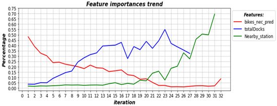
Figure 5. Relative feature importance with the number of iterations of the model.

The feature “Average LB (or UB) observed in the previous two months” (in the table—bikes_nec_pred) is the most important one in the first iterations (low demand), while it becomes irrelevant when the goal is to predict large volumes of bikes (Iteration 32). The opposite trend can be observed for other features, such as the Capacity of the station (in the table—totalDocks), which is not relevant for small demand values but becomes dominant when we deal with large volumes of bikes. Note also that the features Nearby_station and totalDocks became even more correlated, and therefore at Iteration 23, the latter becomes redundant, and it is removed, allowing for the increase in the relevance of the Nearby_station feature.

Thus, while different features can impact different demand levels, general purpose resampling methods would not perceive this difference and therefore would not be able to use the best features during the prediction phase. This is the reason for proposing the iterative resampling approach that provides more flexibility when it comes to feature importance, allowing to capture the difference between features that are good at explaining the majority class, the rare class, or both.

4.4. Prediction of the Upper Bound and Lower Bound for Existing Stations

In this section, the UB and LB are calculated using the methods discussed in Section 2. Specifically, decision trees such as GTBC and RFC are firstly implemented with the features of Table 1.

For clarity of analysis, the results (Figure 6 and Figure 7) are illustrated dividing the class with the low number of bikes from the class with the high number of bikes, where the division was performed according to half of the observed UB/LB. Hence, the MAE values can be compared (Figure 7), highlighting the accuracy for each class. Please note that these classes are not those used to solve the classification exercise. In that case, the classes are defined as discussed in Section 2, assuming $\epsilon =2.$

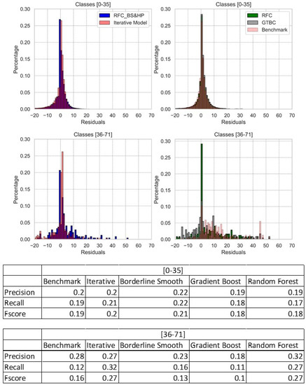
Figure 6. Distribution of the residuals for the LB, Classes (0–35) and (36–71), and related prediction metrics.

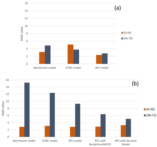
Figure 7. MAE values for the UB (a) and LB (b) with and without resampling for existing stations.

In the UB estimation case, no rebalancing technique was needed since the database was sufficiently balanced. All models, the benchmark included, returned good forecasts of bikes’ UB, nevertheless a slight underestimation is observed (Figure 7a).

With the benchmark model, good predictions are obtained; however, the RFC was the best performing algorithm. Specifically, it adjusted the benchmark estimation by deriving information thanks to the features additionally adopted in the calibration. On the other hand, the GTBC was quite poor, especially with respect to the class with the highest number of bikes; thus, the RFC should be used in this case.

The situation is different for the LB (Figure 6 and Figure 7b). In this case, the database was imbalanced (Table 2) toward the low values of bikes; thus, resampling techniques have been used. These techniques, specifically the BorderlineSMOTE and our proposed iterative model, have been combined with the RFC. The BorderlineSMOTE is the reference model for resampling, as it represents a common method for data imbalance.

As expected for the LB prediction, when looking at the benchmark, at the RFC and the GDBC, the MAE is fairly low for the classes with the highest number of bikes, while it is at least three times larger for the other ones. From the distribution of the residuals for each model (Figure 6), it emerges clearly.

Concerning data unbalancing, we can also observe that both the BorderlineSMOTE and the iterative model perform better than the other models. Nevertheless, the pro-posed iterative model clearly outperforms the BorderlineSMOTE. This is because the Borderline SMOTE shows a smaller error for the dominant class (MAE (0–35)) and a larger error for the minority one (MAE (36–71)), which is a clear indication of the BorderlineSMOTE model overfitting the dominant class.

4.5. Predicting New Stations Using Only Exogenous Variables

One of the main problems when using ML is the lack of endogenous variables. For instance, if a new station appears in the system, the endogenous features presented in Table 1 cannot be used to predict inventory levels. Therefore, in this section, we test the same model as discussed in the previous section but with only exogenous and behavioral features. This model can be used, for instance, to predict the inventory levels when historical data are not available, as in the case of a new station.

Table 3 shows the numerical results. As in the previous case, for the LB calculation, the RFC alone and in combination with the iterative resampling and BorderlineSMOTE has been used to make predictions. As expected, the results look worse than in the previous case, especially for the rare classes (36–71). When looking at the RFC, the MAE is fairly low for (0–35), while it is almost 10 times larger for (36–71), showing that data imbalance becomes more relevant when only exogenous variables are available. Concerning the other models, in this case, the BorderlineSMOTE performs better than the proposed iterative model for the dominant class, while it performs worse in terms of rare classes. This is related to the generalization problem and shows, as for the previous test, the tendency of the model to overfit the dominant class. With or without endogenous variables, the proposed iterative procedure achieves similar results for the minority and majority classes, showing that the model is less sensitive to overfitting. To remove possible collinearity issues and assess how the features affect the model, the approach was tested using different correlation cuts (see Table 4).

Table 3. Results for the LB (with and without resampling) for new stations.

Lower-Bound Models	MAE (0–35)	MAE (36–71)
RFC	4.85	37.83
RFC with BorderlineSMOTE	6.68	9.07
RFC with Iterative Model	8.41	8.36

Table 4. Results for the LB (with and without resampling) for new stations.

	RFC with BorderlineSMOTE		RFC with Iterative Model
Correlation Cut	MAE (0–35)	MAE (36–71)	MAE (0–35)	MAE (36–71)
0.1	6.66	10.67	8.18	8.19
0.3	6.68	9.07	8.41	8.36
0.5	6.73	8.94	8.31	8.43
0.7	6.66	9.40	8.16	8.51
1	6.66	8.81	8.19	8.44
1.2	10.45	21.39	11.43	8.17

Multicollinearity occurs when multiple features utilized by the ML classifier are strongly correlated. When features are correlated, they are unable to individually provide independent predictions for the dependent variable. Instead, they jointly explain a portion of the variance, thereby diminishing their individual statistical significance. In this section, multicollinearity is accounted for by performing hierarchical clustering on the Spearman’s rank-order correlations, picking a threshold, and keeping a single feature from each cluster. As hierarchical clustering computes the information loss associated with aggregating two features, high thresholds will translate into larger clusters and higher information loss. This threshold is called a ‘correlation cut’, and it is one of the parameters of the model that we used to avoid overfitting. As discussed at the beginning of this section, during each iteration, we use feature selection to select which features should be used and which features should be excluded to avoid overfitting. A high correlation cut translates into a model with less features. Intuitively, more features (i.e., a low correlation cut) implies more overfitting while less features (i.e., high correlation cut) lead to poor model performance. The results confirm that the BorderlineSMOTE tends to overfit the dominant class with respect to the minority class and, in general, model performance is heavily influenced by the adopted correlation cut. The proposed iterative model, which makes predictions on an ensemble of classifiers and weights, provides more balanced predictions and an error that is similar for the majority and minority classes. It can also be observed that, for all models, the error is maximum when the correlation cut = 1.2. This is reasonable, as when too many features are grouped together, the model is not able to sufficiently generalize from the data.

4.6. Prediction Based on a Day-to-Day Approach

Finally, we test the model using the day-to-day approach as described in Equation (8). The results are depicted in Table 5. Note that, in this case, the dominant class and the minority class of the lower bound have different values than in the previous experiment (MAE (0–39) and MAE (40–79) instead of MAE (0–35) and MAE (36–71) in Table 3 and Table 4). The reason is that, in this experiment, we use a different dataset. More specifically, this experiment uses data from 2019, while the previous one focused on the number of rides in 2018. The definition of the dominant class in the two experiments is the same. However, the interval is different, which also reflects an increase in the demand for bike-sharing services in 2019 with respect to 2018.

Table 5. Results for the LB (best classifier with iterative resampling model) previsions for new stations.

Lower-Bound Models	MAE (0–39)	MAE (40–79)
RFC with Iterative Model	3.27	4.79

It should be noted that the results are shown only for the iterative model; this is because firstly the comparison between resampling approaches was already presented in the previous subsections. Secondly, the BorderlineSMOTE was extremely time-consuming and not applicable in practice for a day-to-day framework. Therefore, Table 4 only validates what was described before, showing that the proposed formulation is a good method to compute inventory levels and that the iterative approach also performs well in the case of a day-to-day framework.

5. Conclusions

The inventory problem is a challenge for bike-sharing operators. The problem, which consists in estimating the total number of bikes necessary at each bike-sharing station, is complex for two reasons. First, for traditional station-based systems, it is necessary to estimate both the number of bikes as well as the number of bicycles, which makes the problem more complex. Second, the demand for bicycles is sparse, meaning that many stations are empty while a few have very high demand values. While researchers agree that the inventory problem is a key issue, this information is usually obtained from historical data. Therefore, in this paper, we proposed using machine learning (ML) as a more accurate way of extracting this information from historical data. Specifically, we formulate the inventory problem as a classification problem that can be solved using any state-of-the-art classifier ML model. We also developed an iterative resampling technique to deal with the problem of the sparsity of the demand, which is a main problem when using ML classifiers.

The model is tested using real-world data from Citi Bike, the bike-sharing system that is currently in service in New York, US. The model provides estimates for the inventory problem in terms of the upper bound and lower bound of bikes. The results suggest that the proposed approach is robust in terms of results and can be applied in several circumstances, including opening new bike-sharing stations and day-to-day operations. The current research has two main limitations. First, it has been tested on a station-based system. Second, it has been adopted for the solution of the static inventory problem, i.e., estimating during the nighttime the optimal inventory levels for the morning. Future research will therefore focus on testing with different data, different operational settings, and in the case of real-time problems. A relevant future research direction is also to use clustering to identify similar stations. While in this research we focused primarily on resampling, it appears obvious that it is irrelevant to compute the inventory levels for stations that tend to naturally rebalance themselves, therefore requiring no action from the operator. As multiple stations have a lower bound of zero, it would be relevant to use clustering to identify these stations. This would allow to remove these stations from the dataset and remove or at least substantially reduce data imbalance.

References

- Loaiza-Monsalve, D.; Riascos, A.P. Human Mobility in Bike-Sharing Systems: Structure of Local and Non-Local Dynamics. PLoS ONE 2019, 14, e0213106. [Google Scholar] [CrossRef]
- Lahoorpoor, B.; Faroqi, H.; Sadeghi-Niaraki, A.; Choi, S.-M. Spatial Cluster-Based Model for Static Rebalancing Bike Sharing Problem. Sustainability 2019, 11, 3205. [Google Scholar] [CrossRef]
- Fricker, C.; Gast, N.; Mohamed, H. Mean Field Analysis for Inhomogeneous Bike Sharing Systems. Discret. Math. Theor. Comput. Sci. 2012. Available online: https://dmtcs.episciences.org/3006/pdf (accessed on 23 June 2023). [CrossRef]
- Cruz, F.; Subramanian, A.; Bruck, B.P.; Iori, M. A Heuristic Algorithm for a Single Vehicle Static Bike Sharing Rebalancing Problem. Comput. Oper. Res. 2017, 79, 19–33. [Google Scholar] [CrossRef]
- Regue, R.; Recker, W. Proactive Vehicle Routing with Inferred Demand to Solve the Bikesharing Rebalancing Problem. Transp. Res. Part E Logist. Transp. Rev. 2014, 72, 192–209. [Google Scholar] [CrossRef]
- Legros, B. Dynamic Repositioning Strategy in a Bike-Sharing System; How to Prioritize and How to Rebalance a Bike Station. Eur. J. Oper. Res. 2019, 272, 740–753. [Google Scholar] [CrossRef]
- Datner, S.; Raviv, T.; Tzur, M.; Chemla, D. Setting Inventory Levels in a Bike Sharing Network. Transp. Sci. 2019, 53, 62–76. [Google Scholar] [CrossRef]
- Ashqar, H.I.; Elhenawy, M.; Almannaa, M.H.; Ghanem, A.; Rakha, H.A.; House, L. Modeling Bike Availability in a Bike-Sharing System Using Machine Learning. In Proceedings of the 2017 5th IEEE International Conference on Models and Technologies for Intelligent Transportation Systems (MT-ITS), Naples, Italy, 26–28 June 2017; pp. 374–378. [Google Scholar]
- Ruffieux, S.; Spycher, N.; Mugellini, E.; Khaled, O.A. Real-Time Usage Forecasting for Bike-Sharing Systems: A Study on Random Forest and Convolutional Neural Network Applicability. In Proceedings of the 2017 Intelligent Systems Conference (IntelliSys), London, UK, 7–8 September 2017; pp. 622–631. [Google Scholar]
- Ceccarelli, G.; Cantelmo, G.; Nigro, M.; Antoniou, C. Machine Learning from Imbalanced Data-Sets: An Application to the Bike-Sharing Inventory Problem. In Proceedings of the 2021 7th International Conference on Models and Technologies for Intelligent Transportation Systems (MT-ITS), Heraklion, Greece, 16–17 June 2021; pp. 1–6. [Google Scholar]
- Laporte, G.; Meunier, F.; Calvo, R.W. Shared Mobility Systems. 4OR 2015, 13, 341–360. [Google Scholar] [CrossRef]
- Dell’Amico, M.; Hadjicostantinou, E.; Iori, M.; Novellani, S. The Bike Sharing Rebalancing Problem: Mathematical Formulations and Benchmark Instances. Omega 2014, 45, 7–19. [Google Scholar] [CrossRef]
- Santos, G.G.D.; Correia, G.H.D.A. Finding the Relevance of Staff-Based Vehicle Relocations in One-Way Carsharing Systems through the Use of a Simulation-Based Optimization Tool. J. Intell. Transp. Syst. 2019, 23, 583–604. [Google Scholar] [CrossRef]
- Pal, A.; Zhang, Y. Free-Floating Bike Sharing: Solving Real-Life Large-Scale Static Rebalancing Problems. Transp. Res. Part C Emerg. Technol. 2017, 80, 92–116. [Google Scholar] [CrossRef]
- Chemla, D.; Meunier, F.; Calvo, R.W. Bike Sharing Systems: Solving the Static Rebalancing Problem. Discret. Optim. 2013, 10, 120–146. [Google Scholar] [CrossRef]
- Erdoğan, G.; Battarra, M.; Calvo, R.W. An Exact Algorithm for the Static Rebalancing Problem Arising in Bicycle Sharing Systems. Eur. J. Oper. Res. 2015, 245, 667–679. [Google Scholar] [CrossRef]
- Kloimüllner, C.; Papazek, P.; Hu, B.; Raidl, G.R. Balancing Bicycle Sharing Systems: An Approach for the Dynamic Case. In Evolutionary Computation in Combinatorial Optimisation; Lecture Notes in Computer, Science; Blum, C., Ochoa, G., Eds.; Springer: Berlin/Heidelberg, Germany, 2014; pp. 73–84. [Google Scholar]
- Chen, P.; Hsieh, H.; Su, K.; Sigalingging, X.K.; Chen, Y.; Leu, J. Predicting Station Level Demand in a Bike-Sharing System Using Recurrent Neural Networks. IET Intell. Transp. Syst. 2020, 14, 554–561. [Google Scholar] [CrossRef]
- Wang, B.; Vu, H.L.; Kim, I.; Cai, C. Short-Term Traffic Flow Prediction in Bike-Sharing Networks. J. Intell. Transp. Syst. 2022, 26, 461–475. [Google Scholar] [CrossRef]
- Xu, C.; Ji, J.; Liu, P. The Station-Free Sharing Bike Demand Forecasting with a Deep Learning Approach and Large-Scale Datasets. Transp. Res. Part C Emerg. Technol. 2018, 95, 47–60. [Google Scholar] [CrossRef]
- Nair, R.; Miller-Hooks, E. Fleet Management for Vehicle Sharing Operations. Transp. Sci. 2011, 45, 524–540. [Google Scholar] [CrossRef]
- Schuijbroek, J.; Hampshire, R.; van Hoeve, W.-J. Inventory Rebalancing and Vehicle Routing in Bike Sharing Systems. Eur. J. Oper. Res. 2017, 257, 992–1004. [Google Scholar] [CrossRef]
- O’Mahony, E.; Shmoys, D.B. Data Analysis and Optimization for (Citi) Bike Sharing. In Proceedings of the Twenty-Ninth AAAI Conference on Artificial Intelligence, AAAI’15, Austin, TX, USA, 25–30 January 2015; AAAI Press: Washington, DC, USA, 2015; pp. 687–694. [Google Scholar]
- Rudloff, C.; Lackner, B. Modeling Demand for Bikesharing Systems: Neighboring Stations as Source for Demand and Reason for Structural Breaks. Transp. Res. Rec. 2014, 2430, 1–11. [Google Scholar] [CrossRef]
- Ploeger, J.; Oldenziel, R. The sociotechnical roots of smart mobility: Bike sharing since 1965. J. Transp. Hist. 2020, 41, 134–159. [Google Scholar] [CrossRef]
- Moran, M.E.; Laa, B.; Emberger, G. Six scooter operators, six maps: Spatial coverage and regulation of micromobility in Vienna, Austria. Case Stud. Transp. Policy 2020, 8, 658–671. [Google Scholar] [CrossRef]
- Li, L.; Liu, Y.; Song, Y. Factors affecting bike-sharing behaviour in Beijing: Price, traffic congestion, and supply chain. Ann. Oper. Res. 2019, 1–16. [Google Scholar] [CrossRef]
- Jin, Y.; Ruiz, C.; Liao, H. A simulation framework for optimizing bike rebalancing and maintenance in large-scale bike-sharing systems. Simul. Model. Pract. Theory 2022, 115, 102422. [Google Scholar] [CrossRef]
- Jamali, I.; Bazmara, M.; Jafari, S. Feature Selection in Imbalance Data Sets. Int. J. Comput. Sci. Issues 2013, 9, 42. [Google Scholar]
- Orriols-Puig, A.; Bernadó-Mansilla, E. Evolutionary Rule-Based Systems for Imbalanced Data Sets. Soft Comput. 2009, 13, 213–225. [Google Scholar] [CrossRef]
- Krawczyk, B. Learning from Imbalanced Data: Open Challenges and Future Directions. Prog. Artif. Intell. 2016, 5, 221–232. [Google Scholar] [CrossRef]
- Zhou, Z.-H.; Liu, X.-Y. On Multi-Class Cost-Sensitive Learning. Comput. Intell. 2010, 26, 232–257. [Google Scholar] [CrossRef]
- Batista, G.E.A.P.A.; Prati, R.C.; Monard, M.C. A Study of the Behavior of Several Methods for Balancing Machine Learning Training Data. ACM SIGKDD Explor. Newsl. 2004, 6, 20–29. [Google Scholar] [CrossRef]
- Ganganwar, V. An Overview of Classification Algorithms for Imbalanced Datasets. Int. J. Emerg. Technol. Adv. Eng. 2012, 2, 42–47. [Google Scholar]
- Wang, J.; Xu, M.; Wang, H.; Zhang, J. Classification of Imbalanced Data by Using the SMOTE Algorithm and Locally Linear Embedding. In Proceedings of the 2006 8th international Conference on Signal Processing, Guilin, China, 16–20 November 2006; Volume 3. [Google Scholar]
- Dal Pozzolo, A.; Caelen, O.; Johnson, R.A.; Bontempi, G. Calibrating Probability with Undersampling for Unbalanced Classification. In Proceedings of the 2015 IEEE Symposium Series on Computational Intelligence, Cape Town, South Africa, 7–10 December 2015; pp. 159–166. [Google Scholar]
- Liu, X.-Y.; Wu, J.; Zhou, Z.-H. Exploratory Undersampling for Class-Imbalance Learning. IEEE Trans. Syst. Man Cybern. Part B (Cybernetics) 2009, 39, 539–550. [Google Scholar] [CrossRef]
- He, H.; Garcia, E.A. Learning from Imbalanced Data. IEEE Trans. Knowl. Data Eng. 2009, 21, 1263–1284. [Google Scholar] [CrossRef]
- Chen, H.; Li, C.; Yang, W.; Liu, J.; An, X.; Zhao, Y. Deep Balanced Cascade Forest: A Novel Fault Diagnosis Method for Data Imbalance. ISA Trans. 2021, 126, 428–439. [Google Scholar] [CrossRef] [PubMed]
- Cantelmo, G.; Kucharski, R.; Antoniou, C. Low-Dimensional Model for Bike-Sharing Demand Forecasting That Explicitly Accounts for Weather Data. Transp. Res. Rec. 2020, 2674, 132–144. [Google Scholar] [CrossRef]
Disclaimer/Publisher’s Note: The statements, opinions and data contained in all publications are solely those of the individual author(s) and contributor(s) and not of MDPI and/or the editor(s). MDPI and/or the editor(s) disclaim responsibility for any injury to people or property resulting from any ideas, methods, instructions or products referred to in the content. |
© 2023 by the authors. Licensee MDPI, Basel, Switzerland. This article is an open access article distributed under the terms and conditions of the Creative Commons Attribution (CC BY) license (https://creativecommons.org/licenses/by/4.0/).