Abstract
The paper outlines an algorithm for the rapid aerodynamic evaluation of winglet geometries using the TORNADO Vortex Lattice Method. It is a very useful tool to obtain a first approximation of the aerodynamic properties and for performing an optimization of the geometry design. The TORNADO tool is used to systematically calculate the aerodynamic characteristics of various wings with wingtip devices. The fast response of the aerodynamic models allows obtaining a set of results in a remarkably short time. Therefore, the development of an algorithm to generate wing geometries with great ease and complex shapes is of vital importance for the mentioned optimization process. The basic outline of the algorithm, the equations defining the wing geometries, and the results for unconventional wingtip devices, such as blended winglets and spiroid winglets, are presented. Finally, this algorithm allows designing a procedure to study the improvement of aerodynamic properties (lift, induced drag, and moment). Some examples are included to illustrate the capabilities of the algorithm.
1. Introduction
Understanding the aerodynamic properties of a flying vehicle is essential for determining its performance and flight dynamics. These aerodynamic characteristics can be obtained through experimental, computational, and also flight tests. Computational methods can solve the Navier–Stokes equations, including viscosity terms (with high computational cost), or solve the equations with potential models (simplified linearized models). The differential equations used for solving the most relevant problems in low-speed (incompressible) aerodynamics will be a simplified version of the equations governing fluid mechanics, that is, the conservation equations for mass, momentum, and energy (if necessary) [1].
The majority of fluid studies and their engineering applications require a solution within a fluid domain, usually containing a solid body, with a series of boundaries. Theoretical potential aerodynamics models are a reduction of the general equations, so it is important to understand these introduced simplifications. This allows us to appreciate the power and versatility of the models (both analytical and numerical), as well as the limitations imposed by the simplifications themselves.
It is known [1] that at high Reynolds numbers , the dimensions of the boundary layer (inversely proportional to or ) are small, and the effects of viscosity are confined to this thin region attached to the obstacle. Therefore, potential models will predict lift, induced drag, and aerodynamic moment with good approximation but not viscous drag.
Potential aerodynamics is valid outside the boundary layer [1,2], outside the shear layers and wakes, where the viscosity effects are negligible or non-existent; then, outside these regions, the vorticity is zero. The velocity field in potential aerodynamics derives from the potential of velocity , then . That is, the assumptions of the flow will be incompressible motion and zero viscosity. Thus, with these approximate models, it will suffice to solve the continuity equation for incompressible flow and the Euler equation (relationship between pressure p and velocity V, i.e., the Bernoulli equation) [3].
From the theorems of scientist Hermann Von Helmholtz [3] based on vortices for incompressible flow, we can establish that the intensity of a vortex filament is constant along its length, and it cannot start or end in the fluid. A moving fluid forms a vortex tube, and its intensity remains constant to the extent that the tube moves. The induced velocity by a vortex segment is defined by the Biot–Savart law [2,3].
From the aforementioned conditions, it is possible to establish a set of elementary solutions of the Laplace equation . These elementary solutions can be sources, doublets, and vortices [1,2,3]. Being elementary solutions of the Laplace equation, the principle of superposition can be applied, which forms the foundation for solving the fluid field around complex surfaces. The Rankine oval, flow around a cylinder, and flow over a sphere [1] are examples of flows around simple surfaces or bodies. With all of this, it is indicated that the solution of potential flow (incompressible, inviscid) around arbitrary bodies can be determined by distributing elementary solutions over the surfaces to be modeled. In other words, the distributions of sources, the distributions of doublets, and the distributions of vortices can be superposed.
The solution of potential flow could be solved using analytical methods, but obtaining the mentioned solutions is only possible in very specific and limited cases. If appropriate simplifications are made on geometric surfaces (curvature, thickness, etc.), it allows linearizing the problem and applying numerical techniques. There are different software that have been developed in the past years for different applications and that solve the aerodynamic problem using the Navier–Stokes equations for potential flow equations [4,5]. To simulate using the method of small perturbations on a three-dimensional wing, it could be achieved using distributions of singularities (elementary solutions); a horseshoe vortex distribution forms the basis of the VLM method. This way, problems can be solved on three-dimensional lifting surfaces with dihedral, sweep, and even sideslip. This is a generalized solution of Prandtl’s lifting-line theory.
TORNADO uses the vortex lattice method (VLM), which is an aerodynamic analysis at steady state. AVL [6], Surfaces [7], XFLR5 [4] and VSPAERO [8] are also vortex lattice-based and can give good results for preliminary studies. Some articles show the significant evolution and application capacity of these methods, for example, using non-linear VLM [9,10], unsteady VLM (UVLM) [5] or even adapting VLM to supersonic aircraft [11]. From this point on, the focus will be on TORNADO, which was the tool chosen to develop the code due to the simplicity of adapting the program. The wing is supposed to be divided into trapezoidal panels (see Figure 1), each of them with an associated horseshoe vortex. The turbillonary field generated by the vortices is divided in two regions: the free vortices, which cause the induced velocity, and the bound vortices, which are related to the airfoil lift effect. The panels have two important points, the control point in 3/4 of the wing chord (c) and the head of the vortex in 1/4c. Each vortex has a circulation distribution (associated with the induced velocity and the interaction between vortices), which allows to calculate the lift distribution. With that distribution and the angle of attack, the lift and induced drag coefficient can be obtained. The VLM method is one of the most extended methods to calculate aerodynamics properties based on potential features of the flow, that is, lift force, moment and induced drag. The computational effort is extraordinarily low due to the linearized nature of the equations, as well as the final result of solving linear systems of equations (even of large dimensions). According to this, the VLM method has limitations, as it can be applied when low angles of attack are considered (to avoid effects of stall conditions) to ignore the compressibility effects, and it is a method by which any type of drag dependent on viscosity cannot be calculated [12].
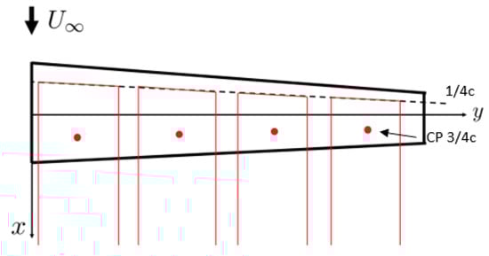
Figure 1.
VLM scheme. In the figure it can be seen the dotted black line 1/4c, and the control points and horseshoes in red. The horseshoes start in line 1/4c and continue downstream.
The wings to be studied in this article are those that introduce wingtip devices. Winglets are becoming increasingly important elements in aircraft design, as operating costs and environmental concerns are on the rise. Therefore, from an aerodynamic point of view, wingtip devices are able to reduce induced drag [13] and increase aerodynamic efficiency. Figure 2 presents different configurations that have been used or are in development.
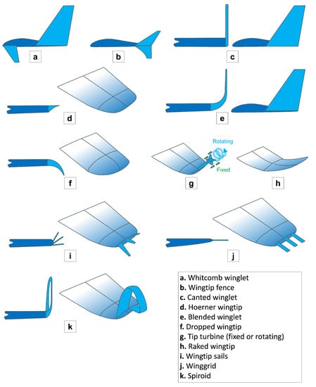
Figure 2.
Winglet configurations that have been used or are in development.
Fredick W. Lanchester was the first person to mention the possibility of creating a vertical surface (end-plate), in the belief that it would reduce drag by controlling wing tip vortices [14]. Later, it was Richard T. Whitcomb who developed the first winglet, with the inspiration of bird wings [15]. One of the conclusions was that the winglets’ presence helped at a Mach number of 0.78, and keeping the lift coefficient from the state without winglets decreased the induced drag about 20% and increased the aerodynamic efficiency about 9% [15]. Another important contribution was made by John M. Kuhlman, who realized a study about the effects that winglets have in low elongation configurations. He concluded that the reduction in the induced drag depends solely on the ratio of the winglet length to the wingspan [16].
Figure 3 shows some winglet examples that are designed with the developed algorithm, such as the blended winglet [17], the spiroid winglet [18,19,20,21,22,23] and a first approximation of the wing grid [24,25,26,27]. They were selected due to the previous investigations conducted in the past years. It is worth noting that companies have already implemented the blended winglet and the grid wing. The blended winglet is the main design adopted by the aeronautical industry for commercial airplanes. Top companies, such as Airbus and Boeing, have implemented those designs for new aircraft models, with satisfactory results in terms of efficiency and fuel consumption [28].
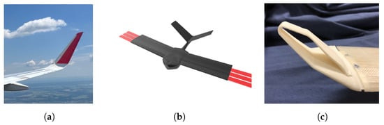
Figure 3.
Details of some of the types of winglets studied. (a) Blended wing. (b) Prototype of a small drone with wing grid (in red). (c) Spiroid.
This paper presents an algorithm that facilitates the wing geometry design to complement the use of TORNADO. The aim of this article is to realize a first iteration of the geometry design of a winglet for its implementation in TORNADO. This software is an extremely valuable tool that offers first-order approximations of performance and lower computational cost than CFD, expediting the optimization of geometry design.
2. Methods
The possibility of using an interface similar to TORNADO is a great help to optimize the design since in the case of CFD, there is a high computational cost, and in the experimental case, it is not feasible to perform all the considered tests but only those that have been previously optimized. TORNADO can give a first approximation to the problem using MATLAB, but it has some limitations, especially when defining the geometry. For that reason, MATLAB is used to provide an algorithm to solve the aerodynamic problem by using some TORNADO functions. In this article, we focus only on the first geometrical part with the calculation of more complex geometries by introducing the winglets mentioned above. This would be almost unthinkable with the TORNADO interface, as it does not allow easy editing of the geometry changes, and the way parameters are given is less intuitive.
The function named WingGeometry.m was developed in MATLAB including an algorithm that allows the user to define a complex wing geometry based on a main wing—taper wing—and the winglets.
2.1. Definition of the Main Wing
The first parameters required are the number of wings () and the number of parts () that each wing has. For simplifying the problem instead of using a x matrix, the numbers of parts are one in each wing, having only a vector x1:
2.1.1. Aircraft Reference Points
There are two points that need to be defined in the code: the aircraft reference point and the gravity center. The first is the point in which the momentums are calculated. As it can be observed in Figure 4 the reference point is placed in [0, 0, 0]m (body axis), and the gravity center at [0.05, 0, 0]m (the middle point of the root chord). The blue line is the mean aerodynamic chord.
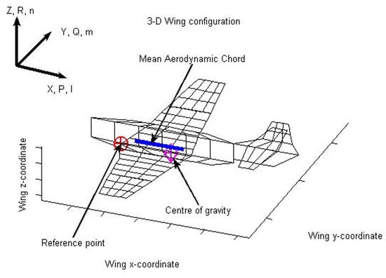
Figure 4.
Example of the reference parameters defined in TORNADO.
2.1.2. Vortex Lattice Method (VLM) Parameters
The wing must be meshed according to the needs for making VLM calculations after the geometry is defined. It has a lot of importance because of the interpolation that is made with the VLM; if the number of panels is not enough, the resulting coefficient solution may not be the correct one as it can be seen in [29]. The parameters for performing the mesh are the number of panels in chord () and in span (), and the mesh type. The main wing has lower complication than the winglets (depending on the winglet shape, it is divided into more components), so the selected values were and . The mesh can have different types in which to place the number of panels (see Figure 5): linear, spanwise half-cosine, spanwise half-cosine/chordwise cosine, and spanwise cosine/chordwise cosine. For the main wing, the linear distribution was considered (). The followed process can be seen in Algorithm 1.
| Algorithm 1 Mesh algorithm. |
|
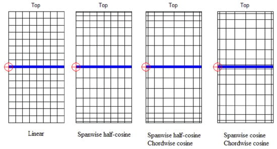
Figure 5.
Mesh types for and . The red dot represents the reference point. The blue line represents the mean aerodynamic chord (mac).
2.1.3. Wing Parameters
For the wing, it is necessary to know the following parameters: wingspan (b), root chord (), taper (), sweep in the point c/4 (), dihedral (), geometric twist and airfoil type (Eppler 186 is used in the main wing). Also, the point where the wing begins has to be defined. For the main wing it will be [0, 0, 0], but for the winglets, their beginning point changes depending on the previous geometry. Finally, it has to be determined whether the wing has symmetry about the XZ plane (see Figure 4).
The building of the geometry struct in TORNADO is made in Algorithm 2. It can be noticed that a vector with the number of wings is made. The vector is used with the winglets in Section 2.2 (e.g., in the blended wing, the winglet can be formed with two wings and a joint between them). The first value is always the value in the root.
| Algorithm 2 Wing parameters algorithm. |
|
2.2. Definition of the Wingtip Devices
For the winglets, it is interesting to notice that the same function WingGeometry.m can be used. In this case, the number of wings is increased depending on the type of winglet that is selected. The different types that can be chosen are (=): no winglet (no winglet), blended (blended), open spiroid (spiroid open) and closed spiroid winglet (spiroid closed).
2.2.1. Blended Winglet
This winglet type is used as the basis of all coding. Each winglet is composed by one or more elements connected to each other and the main wing through joints. The joints aim to provide the winglets with smooth coupling without generating pointed geometries. Each part of the joint is called a component. Due to the greater complexity in this case, the parameters are connected with each other in some cases and with the main wing.
Starting from the known data, the total taper () of the joint can be obtained using the main wing tip chord () and the winglet root chord (). See Equation (2):
With and the component number (in the algorithm, this is the number of wings), the taper (Equation (3)) and the chord of each component can be calculated (Equation (4)):
The dihedral () and the sweep () in the point c/4 have the same calculation by changing the parameter. The winglet dihedral () is known. The total dihedral of the joint (), the dihedral increase () and the dihedral in each component () are calculated with Equations (5)–(7), respectively.
The winglet semi-span is known, and the one in each component is calculated with the radius according to (), and the number of components with the following Equation (8):
The structure of the winglet can be seen in Figure 6.
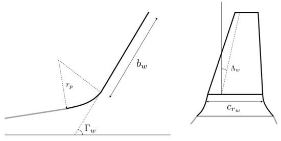
Figure 6.
Detail of the blended winglet structure.
The winglet is supposed to not have a twist. Finally, following the same steps as in the main wing, the type of airfoil can be selected. NACA0012 is used for the winglets.
The new setting that has to be made with the winglets is to define the start of the next component. Using Figure 7 and Figure 8, the component , , and coordinates can be calculated with Equations (9)–(11).
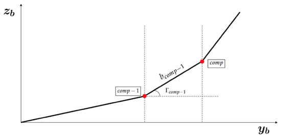
Figure 7.
Scheme used for obtaining and coordinates.
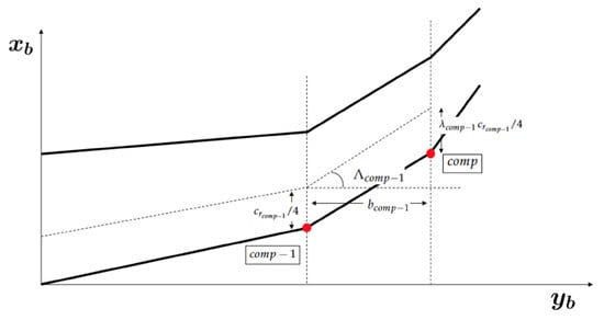
Figure 8.
Scheme used for obtaining coordinate.
The algorithm for the blended winglet can be seen in Algorithm 3.
2.2.2. Open and Closed Spiroid Winglet
Both winglets have the same configuration as the blended winglets but with more joints, which increases the complexity (see Figure 9).
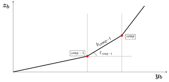
Figure 9.
Detail of the sequential joints. The black dotted points are refered to the different components and the red points to the joint between them.
The structure of the different winglets can be seen in Figure 10 and Figure 11. It is important to mention that the last joint with the closed spiroid has to be with the main winglet, and the process that is represented in Figure 9 is followed backwards.
| Algorithm 3 Blended winglet parameters algorithm. |
|
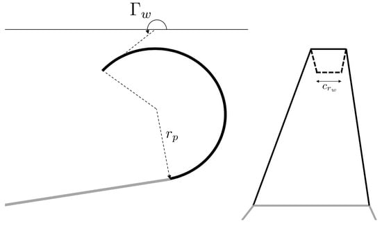
Figure 10.
Detail of the open spiroid winglet structure.
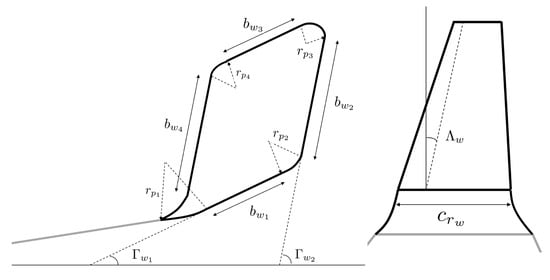
Figure 11.
Detail of the closed spiroid winglet structure.
The programming of the last joint can be seen in Algorithm 4.
| Algorithm 4 Blended winglet parameters algorithm. |
|
3. Results and Discussion
3.1. Algorithm Implemented in TORNADO
After describing the algorithms used for obtaining the complete wing geometry, this section includes the results of the defined geometries. Different types of representation for the geometry can be obtained. The TORNADO function that is used to obtain the representation of the geometry was implemented for the structures that were built with the algorithms. It includes views of the 3D model, the shape of the vortices and different points of view of the 2D model.
Figure 12 shows the different 2D views in addition to the 3D (ISO), side and top views that are obtained with the algorithm from the different type of winglet considered. From the front view, the difference can be seen between not having the winglet and the changing of the joints with the winglet type. The side and ISO views give the winglet details with the number of components. The parts that have an according radius have more components because the part of the wing–winglet joint that is more complicated needs to have more panels for its study. In the main wing and the winglets, the linear distribution can be seen more clearly and is spaced. About the computational cost of the developed algorithm, which was commented on before, the necessary time to compile the blended wing is 3.2 s, while the closed spiroid winglet is 22.1 s. It can be noticed that there is an increase in the time as the geometry gets more complex. With CFD (see Section 3.2), the time increases to 232 s, so for obtaining the optimal geometry, it is better to use the proposed algorithm.
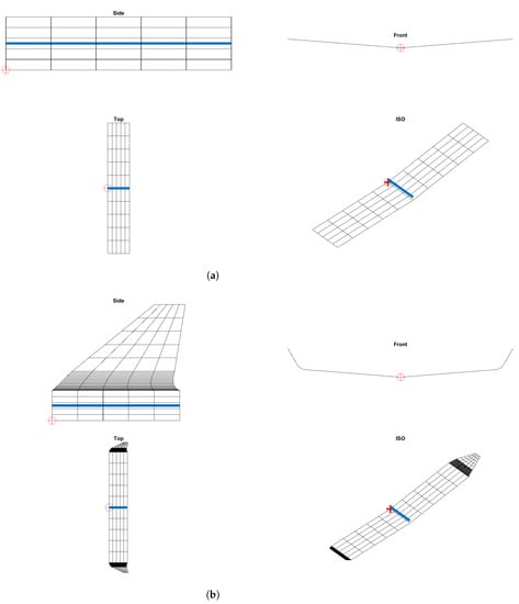
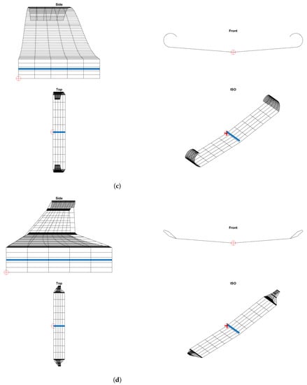
Figure 12.
Depictions of different types of views from the types of winglets used. (a) No winglet. (b) Blended winglet. (c) Open spiroid winglet. (d) Closed spiroid winglet.
In Figure 13, the different 3D views of the complete wing are presented. In this view, the components, wing and winglets are observed. Figure 13b–d are the configurations with winglets, so when the curve part starts, the components of the joints between the wing and winglet can be seen. It can be noticed that for the open spiroid, the components are distributed in a more progressive way since the turn is smoother. The blended and the closed spiroid winglets have closer joints when the winglet starts since the turn is more aggressive.
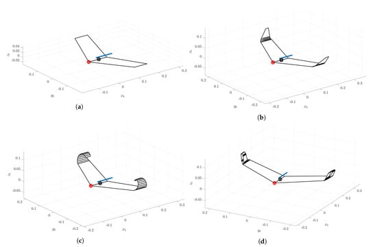
Figure 13.
Details of the 3D view for the types of winglets studied. (a) No winglet. (b) Blended winglet. (c) Open spiroid winglet. (d) Closed spiroid winglet.
Finally, TORNADO has also the option to represent an estimation of the vortex and the wake structure. Those results are collected in Figure 14, and they depend on the number of panels that are used for dividing the wing structure. The red lines show the structure that the wake will follow. The concentration of these red lines at the ends means the concentration of the vortex in those areas. A first early conclusion can be observed in Figure 14c,d; they both can change the vortex size, helping in reducing the induced drag.
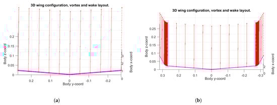
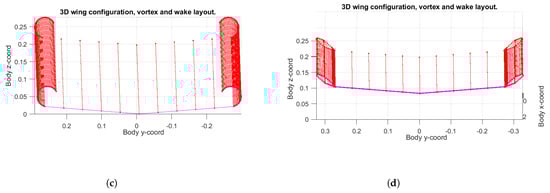
Figure 14.
Details of the vortex and wake structure for the types of winglets studied. (a) No winglet. (b) Blended winglet. (c) Open spiroid winglet. (d) Closed spiroid winglet.
3.2. CFD Comparisons
After the geometry was defined, Ansys-Fluent was used to perform a detailed study of the closed spiroid winglet. The results of the aerodynamic coefficients were calculated for the reference wing without winglets, the closed spiroid winglet for TORNADO and the closed spiroid winglet for Ansys-Fluent (see Table 1). Experimental study of the wing without the winglet and the closed spiroid winglet was also conducted because of the TORNADO limitations specified before; the coefficients for the first case are collected in the table.

Table 1.
Aerodynamic coefficients (lift coefficient, ; drag coeffient, ) and efficiency, E; calculated for the reference wing without winglets and the closed spiroid winglet for TORNADO, Ansys-Fluent and experimental.
It can be seen from the table that TORNADO has problems with the coefficients. For the drag coefficient, as it was explained before, only the induced drag is obtained. The lift coefficient for the reference wing has a good approximation but for the closed spiroid winglet, it differs more, which happens because of the complexity of the geometry in the winglet. The results that are interesting are the closed spiroid winglet with Ansys-Fluent and the experimental results using the reference wing because they are obtained with reliable methods (the purpose of using TORNADO was only to obtain the final geometry). It can be seen that the closed spiroid winglet reduces the drag coefficient and increases the efficiency as wanted.
4. Conclusions
Although TORNADO encounters challenges in two specific cases (the study of the separation point and the overall calculation of the drag coefficient), it is a very useful tool, as evidenced in this article, and the winglet primarily affects induced drag (the studied one). The algorithm implementation achieved the aim of the article: to make an algorithm that can create complex geometry in TORNADO using a basic data entry mechanism and to obtain the optimal geometry with very low computational cost before using CFD. Moreover, the algorithm allows the automation of the winglet generation process selecting basic wing characteristics, such as the root and tip chord, the airfoil, tape, dihedral, the winglet type, panel distribution, number of joints, and the according radius, among others.
In addition, in order to complete the drag reduction study, TORNADO has the capability to calculate the lift and induced drag coefficients. This may lead to the development of a new algorithm (e.g., genetic algorithm) to determine the optimal winglet during the initial design. The final winglet design could then be subject to CFD and experimental analysis for validation. Therefore, this article provides a solid basis for the subsequent phases of winglet development.
Author Contributions
Conceptualization, Á.A.R.-S., R.B.-M., A.L.-C.-A. and D.A.-M.; Methodology, Á.A.R.-S., A.L.-C.-A. and D.A.-M.; Software, A.L.-C.-A., D.A.-M., J.C.M.-G., E.B.-B. and J.F.-A.; Validation, Á.A.R.-S., R.B.-M., A.L.-C.-A., D.A.-M., J.C.M.-G., E.B.-B. and J.F.-A.; Formal Analysis, Á.A.R.-S. and R.B.-M.; Investigation, Á.A.R.-S., R.B.-M., A.L.-C.-A., D.A.-M., J.C.M.-G., E.B.-B. and J.F.-A.; Resources, R.B.-M. and D.A.-M.; Data Curation, R.B.-M.; Writing—Original Draft Preparation, Á.A.R.-S. and A.L.-C.-A.; Writing—Review and Editing, Á.A.R.-S., R.B.-M., A.L.-C.-A., D.A.-M., J.C.M.-G., E.B.-B. and J.F.-A.; Visualization, D.A.-M.; Supervision, Á.A.R.-S. and R.B.-M.; Project Administration, Á.A.R.-S. and R.B.-M. All authors have read and agreed to the published version of the manuscript.
Funding
This research received no external funding.
Institutional Review Board Statement
Not applicable.
Informed Consent Statement
Not applicable.
Data Availability Statement
Not applicable.
Acknowledgments
Not applicable.
Conflicts of Interest
The authors declare no conflict of interest.
Abbreviations
The following abbreviations are used in this manuscript:
| CFD | Computational fluid dynamics |
| Number of wings | |
| Number of parts | |
| VLM | Vortex Lattice Method |
| LD | Linear dichroism |
| Number of panels in chord | |
| Number of panels in semi-span | |
| b | Wingspan |
| Root chord | |
| Wing taper | |
| Wing sweep | |
| Wing dihedral | |
| Total | |
| w | Wing |
| Component | |
| Increment | |
| Radius according |
References
- White, F.M. Fluid Mechanics; McGraw Hill: New York, NY, USA, 1990. [Google Scholar]
- Bertin, J.J.; Cummings, R.M. Aerodynamics for Engineers; Cambridge University Press: Cambridge, UK, 2021. [Google Scholar]
- Katz, J.; Plotkin, A. Low-Speed Aerodynamics; Cambridge University Press: Cambridge, UK, 2001; Volume 13. [Google Scholar]
- Yu, F.; Bartasevicius, J.; Hornung, M. Comparing Potential Flow Solvers for Aerodynamic Characteristics Estimation of the T-FLEX UAV. In Proceedings of the 33rd Congress of the International Council of the Aeronautical Sciences, Stockholm, Sweden, 4–9 September 2022. [Google Scholar]
- Roccia, B.A.; Preidikman, S.; Massa, J.C. Modified Unsteady Vortex-Lattice Method to Study Flapping Wings in Hover Flight. AIAA J. 2013, 51, 2628–2642. [Google Scholar] [CrossRef]
- Official Website of the Product AVL. Available online: http://web.mit.edu/drela/Public/web/avl/ (accessed on 22 August 2023).
- Surfaces—Vortex-Lattice Module; Great OWL Publishing: Ephrata, PA, USA, 2009.
- Official Website of VSPAERO. Available online: https://openvsp.org/wiki/doku.php?id=vspaerotutorial (accessed on 22 August 2023).
- Gabor, O.S.; Koreanschi, A.; Botez, R.M. A new non-linear Vortex Lattice Method: Applications to wing aerodynamic optimizations. Chin. J. Aeronaut. 2016, 29, 1178–1195. [Google Scholar] [CrossRef]
- Rom, J.; Melamed, B.; Almosnino, D. Experimental and Nonlinear Vortex Lattice Method Results for Various Wing-Canard Configurations. J. Aircr. 1993, 30, 207–212. [Google Scholar] [CrossRef]
- Joshi, H.; Thomas, P. Review of vortex lattice method for supersonic aircraft design. Aeronaut. J. 2023, 1–35. [Google Scholar] [CrossRef]
- Melin, T. User’s Guide and Reference Manual for Tornado; Royal Institute of Technology (KTH): Stockholm, Sweden, 2000. [Google Scholar]
- Kroo, I. Drag due to lift: Concepts for prediction and reduction. Annu. Rev. Fluid Mech. 2001, 33, 587–617. [Google Scholar] [CrossRef]
- Jupp, J. Wing aerodynamics and the science of compromise. Aeronaut. J. 2001, 105, 633–641. [Google Scholar] [CrossRef]
- Whitcomb, R.T. Langley Research Center and United States. A Design Approach and Selected Wind Tunnel Results at High Subsonic Speeds for Wing-Tip Mounted Winglets; National Aeronautics and Space Administration: Washington, DC, USA, 1976. [Google Scholar]
- Kuhlman, J.M.; Liaw, P. Winglets on low-aspect-ratio wings. J. Aircr. 1988, 25, 932–941. [Google Scholar] [CrossRef]
- Gratzer, J.L.B. Blended Winglet. U.S. Patent 5,348,253, 20 September 1994. [Google Scholar]
- Gratzer, J.L.B. Spiroid-Tipped Wing. U.S. Patent 5,102,06, 7 April 1992. [Google Scholar]
- Nazarinia, M.; Soltani, M.R.; Ghorbanian, K. Experimental study of vortex shapes behind a wing equipped with different winglets. J. Aerosp. Sci. Technol. 2006, 3, 1–20. [Google Scholar]
- Wan, T.; Lien, K.W. Aerodynamic efficiency study of modern spiroid winglets. J. Aeronaut. Astronaut. Aviat. 2009, 41, 23–29. [Google Scholar]
- Gavrilović, N.N.; Rašuo, B.P.; Dulikravich, G.S.; Parezanović, V.B. Commercial aircraft performance improvement using winglets. FME Trans. 2015, 43, 1–8. [Google Scholar] [CrossRef]
- Mostafa, S.; Bose, S.; Nair, A.; Abdul Raheem, M.; Majeed, T.; Mohammed, A.; Kim, Y. A parametric investigation of non-circular spiroid winglets. EPJ Web Conf. 2014, 67, 02077. [Google Scholar] [CrossRef]
- Guerrero, J.E.; Dario Maestro, D.; Bottaro, A. Biomimetic spiroid winglets for lift and drag control. Comptes Rendus Mec. 2012, 340, 67–80. [Google Scholar] [CrossRef]
- La Roche, U. Wing with a Wing Grid as the End Section. U.S. Patent 5,823,480, 20 October 1998. [Google Scholar]
- La Roche, U.; La Roche, H.L. Induced drag reduction using multiple winglets, looking beyond the prandtl-munk linear model. In Proceedings of the 2nd AIAA Flow Control Conference, Portland, OR, USA, 28 June–1 July 2004; p. 2120. [Google Scholar]
- Shelton, A.; Tomar, A.; Prasad, J.V.R.; Smith, M.; Komerath, N. Active multiple winglets for improved unmanned-aerial-vehicle performance. J. Aircr. 2006, 43, 110–116. [Google Scholar]
- Bennett, D.; Covert, E.; Oliver, T. The Wing Grid: A New Approach to Reducing Induced Drag; Massachusetts Institute of Technology: Cambridge, MA, USA, 2001. [Google Scholar]
- Faye, R.; Laprete, R.; Winter, M. Blended Winglets; Aero, Boeing: Arlington, VR, USA, 2002. [Google Scholar]
- Liu, H. Linear Strength Vortex Panel Method for NACA 4412 Airfoil. IOP Conf. Ser. Mater. Sci. Eng. 2018, 326, 012016. [Google Scholar] [CrossRef]
Disclaimer/Publisher’s Note: The statements, opinions and data contained in all publications are solely those of the individual author(s) and contributor(s) and not of MDPI and/or the editor(s). MDPI and/or the editor(s) disclaim responsibility for any injury to people or property resulting from any ideas, methods, instructions or products referred to in the content. |
© 2023 by the authors. Licensee MDPI, Basel, Switzerland. This article is an open access article distributed under the terms and conditions of the Creative Commons Attribution (CC BY) license (https://creativecommons.org/licenses/by/4.0/).