Abstract
Heart rate variability (HRV) has emerged as an essential non-invasive tool for understanding cardiac autonomic function over the last few decades. This can be attributed to the direct connection between the heart’s rhythm and the activity of the sympathetic and parasympathetic nervous systems. The cost-effectiveness and ease with which one may obtain HRV data also make it an exciting and potential clinical tool for evaluating and identifying various health impairments. This article comprehensively describes a range of signal decomposition techniques and time-series modeling methods recently used in HRV analyses apart from the conventional HRV generation and feature extraction methods. Various weight-based feature selection approaches and dimensionality reduction techniques are summarized to assess the relevance of each HRV feature vector. The popular machine learning-based HRV feature classification techniques are also described. Some notable clinical applications of HRV analyses, like the detection of diabetes, sleep apnea, myocardial infarction, cardiac arrhythmia, hypertension, renal failure, psychiatric disorders, ANS Activity of Patients Undergoing Weaning from Mechanical Ventilation, and monitoring of fetal distress and neonatal critical care, are discussed. The latest research on the effect of external stimuli (like consuming alcohol) on autonomic nervous system (ANS) activity using HRV analyses is also summarized. The HRV analysis approaches summarized in our article can help future researchers to dive deep into their potential diagnostic applications.
1. Introduction
Heart rate variability, often known as HRV, measures time fluctuation corresponding to two consecutive heartbeats [1]. This fluctuation is estimated by measuring the distance between succeeding R-peaks (RR interval) of the electrocardiogram signals, resulting in the generation of the RR interval or HRV features [2]. HRV is denoted to reflect the heart’s ability to adapt to changing circumstances by recognizing and responding quickly to different stimuli. HRV features can be used as a valuable marker of cardiac autonomic function. It provides information on the autonomic nervous system (ANS) state, which helps to tune the circulatory system and heart, thereby inducing a natural fluctuation in the heart rate (HR) [3]. The ANS encompasses the parasympathetic nervous system (PNS) and the sympathetic nervous system (SNS). Together, these branches are responsible for controlling the heart rate. Increased activity of SNS or decreased activity of PNS causes cardio-acceleration. Contrastingly, cardio-deceleration can be caused by two different reasons: increased PNS activity and decreased SNS activity.
In the last few decades, there has been a growing consciousness in the scientific community to understand the connection between the ANS and cardiovascular pathophysiology that may lead to cardiac morbidity and mortality due to cardiac failure [4,5,6]. In many recent published studies, HRV has been highlighted as a marker of overall cardiac well-being, which may be explored as a diagnostic tool. The measurements of HRV are easy to perform [1]. It does not require any invasive procedure. HRV analysis reliability is dependent on the consistency in ECG recording conditions, electrode placement, and ECG signal quality [7]. An HRV analysis is usually performed using the time and frequency domain linear approaches. Nevertheless, various researchers have considerably explored the application of some non-linear methods like recurrence and Poincare plots for HRV analyses. In recent years, new dynamic procedures of HRV measurement (e.g., Lyapunov exponents [8], approximation entropy (ApEn) [9], and a detrended fluctuation analysis (DFA) [10]) have been proposed to detect the complex variations in HRV features, providing deeper comprehension of an HRV analysis.
An analysis of HRV features has allowed clinicians to identify a diverse range of abnormalities, illnesses, and possible indications of impending death. For example, Kim et al. (2018) described that an HRV analysis can function as a label for psychological stress when necessary [2]. HRV has been explored for monitoring car drivers’ drowsiness, exhaustion, and anxiety levels [11]. Similarly, an HRV analysis has also found applications in detecting athletic performance and fatigue and assessing depression, anxiety, and other chronic conditions [12]. It has also been reported that HRV can correlate between a sedentary life and a person’s mental/physical well-being. The current study reviews various signal processing strategies used for processing and analyzing HRV features, popular ML models employed in association with HRV features for classifying pathologies, and the different applications of HRV research.
2. Generation of RR Interval Time Series
HRV denotes the RR interval time sequence resulting from an ECG signal. The process requires the recognition of the QRS complex from the ECG signal. Various techniques have been developed for detecting the QRS waves, like Pan-Tompkin’s algorithm [13,14] and wavelet transform-based algorithms [15]. Pan-Tompkin’s algorithm analyzes the angle, amplitude, and QRS width using a sequence of filters and mathematical operators. The process includes band-pass filtering, derivative, squaring, integration, and adaptive thresholding. The block diagram representation of QRS complex recognition using Pan-Tompkin’s system is shown in Figure 1. On the other hand, the wavelet transform-based approach involves the disintegration of the ECG signals using a suitable mother wavelet followed by reconstruction using the required sub-bands [15]. Then, the envelope is computed, smoothing is performed, and peak detection takes place to extract the QRS complexes.
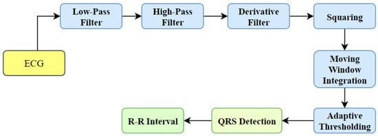
Figure 1.
QRS complex detection using Pan-Tompkin’s algorithm.
Historically, the examination of HRV has been conducted using conventional ECG recordings, which typically have a duration of several minutes or longer. Nevertheless, technological progress has facilitated the acquisition of ultra-short ECG recordings, characterized by significantly shorter durations ranging from 10 s to 150 s [16]. The appeal of ultra-short recordings lies in their convenience and efficiency, rendering them more viable in specific contexts, including ambulatory monitoring, remote patient monitoring, and wearable devices.
A predicament arises when attempting to compare the outcomes derived from ultra-short ECG recordings with those acquired from normal ECG recordings. There exist multiple aspects that contribute to the issue of comparability.
- Signal quality can be compromised in ultra-short ECG recordings as a result of a shorter length, leading to the presence of noise, artifacts, and a reduction in signal quality [17,18]. The potential consequences of this phenomenon include potential inconsistencies in an HRV analysis when compared to standard recordings, which may compromise the accuracy of the results.
- An HRV analysis can be conducted through two distinct approaches, namely a time-domain analysis and frequency-domain analysis [19]. The selection of the analytical approach can have an impact on the outcomes and the capacity to compare ultra-short recordings with regular recordings.
- The examination of HRV in research often operates under the assumption that the fundamental physiological mechanisms remain constant during the duration of the recording [2]. The validity of this premise may be compromised when dealing with long-term recordings, as the longer duration could potentially impact the outcomes due to motion artifacts, electrode movements, signal drift, and patient movements, etc. [2].
- The statistical power of ultra-short recordings may be diminished due to a restricted number of data points, resulting in a decrease in comparison to lengthier conventional recordings. The data points are representative of the voltage measurements acquired from the electrodes positioned on the body. The frequency spectrum of the ECG data depicts the allocation of various frequencies that are present within the signal [20]. Increased recording duration leads to enhanced frequency resolution, enabling the detection and capture of lower-frequency elements of the cardiac signal, including the T-wave and QRS complex.
- The identification and rectification of artifacts in recordings can vary depending on whether the recordings are ultra-short or standard in duration, resulting in discrepancies in the resulting heart rate variability (HRV) measures [16].
In order to effectively tackle these concerns and enhance the level of comparison, scholars have the option of employing diverse methodologies, such as the following:
- Standardization refers to the establishment of rules and protocols that dictate the proper procedures for conducting a heart rate variability (HRV) analysis on ultra-short recordings [21]. The purpose of standardization is to ensure uniformity in the methods employed across different studies and platforms.
- Validation Studies: This research aims to compare the measures of heart rate variability (HRV) derived from ultra-short recordings with standard recordings in the same individuals. The purpose is to assess the level of agreement and identify any potential inconsistencies between the two methods [22].
- The application of data augmentation techniques enables the generation of lengthier recordings from ultra-short segments, hence expanding the available dataset for analysis purposes [23].
The resolution of the comparability issue is crucial in order to maintain the use and dependability of an HRV analysis using ultra-short ECG records for clinical and research purposes. It is imperative for researchers and practitioners to possess a comprehensive understanding of the constraints and difficulties linked to ultra-short recordings, while simultaneously persisting in their exploration of the potential advantages they offer.
3. Pressure Support Ventilation (PSV)
The procedure of adapting raw information into numerical attributes that can be employed in place of the original data is referred to as feature extraction. It helps to reduce the computational burden during a signal analysis while maintaining the integrity of the data confined to the original statistics. The feature extraction from HRV data is commonly accomplished using various methods, including but not limited to (i) time-domain methods, (ii) frequency-domain methods, and (iii) non-linear methods. The HRV features extracted from both time and frequency domain approaches are considered linear HRV features [24].
The linear HRV characteristics are studied following the international guidelines made available by the North American Society of Pacing and Electrophysiology task force and the European Society of Cardiology [6]. On the other hand, the non-linear HRV features are calculated per the recommendations presented in the most recent research literature [25,26,27]. Apart from the methods mentioned above, researchers have also attempted to extract proper HRV parameters using signal decomposition techniques and time-series modelling techniques [28]. The following subsections describe the popular HRV feature extraction methods.
3.1. Time-Domain Methods
The time-domain HRV parameter extraction methods comprise the geometrical and statistical methods [6]. The statistical methods provide the parameters derived either explicitly from the RR intervals or indirectly after the alteration in the length of the RR intervals [29]. Parameters like standard deviation (SD) of the heart rate (HR SD), average heart rate, mean of the NN intervals (or RR intervals), and standard deviation of the NN intervals (SD NN) can be attained straight from the RR intervals. In this instance, the constraints HR SD and SD NN reveal details related to the dispersion of the HR and NN intermission values from their respective mean values. Conversely, the statistical constraints RMSSD, NN50, and pNN50 offer additional material about the high-frequency aberration in the HR. These parameters are based on the variances amid the RR intervals. The root-mean-square standard deviation, or RMSSD, is the average variation in the intermission between beats and is represented by the square root of the consecutive variance involving the RR intervals. The value of NN50 reveals data regarding the number of successive NN interval differences with more than 50 milliseconds. The value of the parameter pNN50 can be calculated by dividing NN50 by the overall number of NN intervals that are longer than 50 milliseconds. TINN, which stands for “triangular interpolation of NN interval histogram,” and the HRV triangular index, are examples of time-domain geometrical parameters. TINN denotes the reference size of the RRI (or NN intermission) histogram when it is calculated using triangular interpolation [30]. The HRV triangular index is obtained from the RRI histogram (Figure 2) by computing the proportion of the entire amount of RRIs to the stature of the RRI histogram [6].
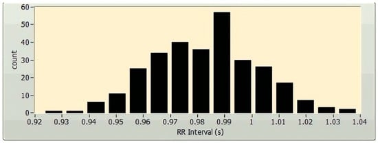
Figure 2.
A sample histogram of a 5 min HRV, plotted using LabVIEW (National Instruments Corporation, Austin, TX, USA).
3.2. Frequency-Domain Methods
The frequency-domain technique uses the estimation of power spectral density (PSD) of the HRVs as the basis for the parameter’s extraction. The parameters of the frequency domain are determined through the application of the Fast Fourier transform (FFT) (Figure 3) and autoregressive modelling (AR) (Figure 4). The PSDs of the very low frequency (VLF; 0.003–0.04 Hz), the low frequency (LF; 0.04–0.15 Hz), and the high frequency (HF; 0.15–0.4 Hz) are considered as the frequency domain HRV features. Absolute power components, like ms2, and relative power components, such as percent, are typically used to measure the VLF, LF, and HF power components, respectively. However, one may also use the normalized units to measure the LF and HF components (n.u.). The power dispersal over numerous constituents of the PSD is unfixed and changes with the autonomic variation of the heart [6]. This is because the PSD is not a fixed function. It has not been determined what precise functional procedure is accountable for producing the VLF power constituent [6], but research is continuing in this direction. Atropine has been reported to eliminate the VLF component. As a result, the VLF power constituent is regarded as a pointer of parasympathetic commotion [29]. Nevertheless, the nature of the LF power constituent is complicated. Both sympathetic and parasympathetic nerve innervations influence the LF power [29]. This makes the LF power component a problematic variable to analyze. Accordingly, the LF/HF proportion is generally utilized to describe the sympathetic activity [29] or the sympathovagal balance [31] rather than the LF power component.

Figure 3.
A typical FFT spectrum of a 5 min HRV, plotted using LabVIEW.

Figure 4.
A typical AR spectrum of a 5 min HRV, plotted using LabVIEW.
3.3. Non-Linear Methods
The heart has been represented as an intricate control system [32]. Hence, the HRV description, which relies solely on linear methods, is insufficient to analyze the signals in many cases. Hence, non-linear approaches are also suggested to represent the HRVs’ properties [32]. Popular non-linear methods include the Poincare plot, detrended fluctuation analysis (DFA), and recurrence plot. The Poincare plot visually represents the correlation between the consecutive RRIs (Figure 5). In the Poincare plot, an ellipse is drawn along the line of identity, and then it is tailored to the statistics points. The width (SD1) and the length (SD2) of the ellipse are used to calculate two non-linear HRV features. Such values are used as indicators of both short- and long-term variance [33].
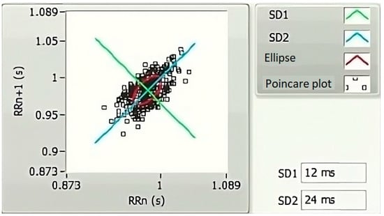
Figure 5.
A representative Poincare graph of a 5 min HRV, plotted using LabVIEW.
Various non-linear techniques exist for quantifying the correlations in nonstationary physiological time series data [34]. The DFA method, developed in the 1970s, is a technique divulging correlation information. In the context of the HRV study, associations are split up into short-term and long-term variations, depending on the time frame under consideration. These variations are measured and quantified with the DFA method using parameters like alpha1 (α1) and alpha2 (α2), respectively [30]. The slope of the log–log graph is utilized to determine the parameters α1 and α2. These values offer a measurement of association (in terms of fluctuation, Fn) that is dependent on the amount of collected data (n) (Figure 6).
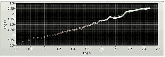
Figure 6.
A representative DFA plot of a 5 min HRV, plotted using LabVIEW. The x-axis of a DFA plot indicates the logarithmically scaled window widths, also known as time scales. Meanwhile, the y-axis represents the logarithmically scaled root-mean-square variation of the detrended data. The analysis of the slope of the plot offers valuable insights into the existence and characteristics of correlations within the examined HRV time series data.
Poincare introduced the concept of recurrence at the end of the 19th century. Recurrence is a fundamental characteristic of every deterministic dynamic scheme [35]. It refers to the phenomenon in which the stages of a dynamic scheme repeatedly appear in phase space [36]. A phase space plot is an imaginary multi-dimensional region where in every point indicates a state of the system. Taken’s theorem [37] has served as the foundation for reconstructing the phase region graphs of the dynamical systems. The theorem proposes that if a variety of parameters governs the dynamics of a system, but a solitary parameter is recognized, at that point, the solitary parameter can still represent the entire dynamics of the system. However, the prediction of the entire system dynamics requires drawing a graph using the quantities of the recognized parameter compared to themselves for a definite amount of times at a predetermined time delay. The selection of appropriate quantities for the embedding dimension and the time delay plays a significant role during the rebuilding of the phase space graph of a dynamic arrangement. The visualization of the vital recurrence property of a phase space plot in two dimensions (2D) has been reported by Eckmann et al. (1987), from whom the idea of recurrence plots was proposed [38]. A recurrence graph is typically described as a symmetrical square matrix in two dimensions. This matrix illustrates the time at which two states of the arrangement become state–space neighbors depending on a cut-off threshold space. However, the information that can be gleaned from this graph is quality-based [39,40]. A recurrence quantification study (abbreviated as RQA) is developed to extract quantity-based variables out of the recurrence plot. The concentration of the reappearance loci and the diagonal, vertical, and horizontal lines present in the recurrence plot are employed for the extraction of quantitative parameters using the RQA method. The popular signal parameters extracted using the RQA method include the recurrence rate (RR), the average number of neighbors (AN), determinism (DET), the length of the longest diagonal line (Lmax), entropy (ENT), laminarity (LAM), trapping time (TT), the maximum length of vertical lines (Vmax), the average length of diagonal lines (AD), the ratio of determinism to the recurrence rate (RATIO), and so on [41].
Chaos theory, a mathematical discipline concerned with the study of intricate and unpredictable systems, has also been used for HRV feature extraction. The utilization of chaos theory principles, including fractals and non-linear dynamics, has been employed in the examination of the intricacy and fluctuation of patterns in HRV [42]. Lyapunov exponents are a sophisticated mathematical construct that originate from the field of chaos theory. These notions find utility in the realm of HRV feature extraction, enabling a deeper understanding of the intricate dynamics inherent in the cardiovascular system. The metric quantifies the speed at which neighboring trajectories in a dynamical system either move apart or come together. A Lyapunov exponent with a larger positive value signifies the presence of chaotic dynamics, whereas a Lyapunov exponent with a negative value shows convergence towards a stable attractor. Through the utilization of Lyapunov exponents derived from time series data of HRV, scholars are able to evaluate the presence of chaotic patterns or ascertain the degree of determinism and stability within the dynamics of heart rate. The provided information can be utilized to gain insights into the regulatory mechanisms of the autonomic nervous system on the heart rate and to detect possible anomalies in cardiovascular well-being [43].
3.4. Signal Decomposition Methods
3.4.1. Empirical Mode Decomposition (EMD)
EMD is a comparatively recent signal processing method utilized to decay the signals into their parts. The processing of non-linear and nonstationary signals is one of its many applications [44]. In this method, the principal (basis) functions are deduced out of the signal, contrasting the Fourier transform or the wavelet transform, which has a fixed basis function. A process known as sifting is implemented in the EMD method to break down a signal into many intrinsic mode functions (IMFs) and a residue (Equation (1)) [45].
The IMFs are a collection of AM-FM (amplitude-modulated–frequency-modulated) signal constituents. They fulfil two criteria: (i) the count of maximum and minimum points has to be similar or slightly differ by one to the count of zero crossings, and (ii) the mean of the covers designed by linking local maxima and minima of the signal is null [46]. Many researchers have reported using the EMD method to decompose the HRVs to extract useful parameters [47]. This may be attributed to the non-linear and nonstationary nature of the HRV features [42].
where M signifies the amount of IMFs, fk(t) shows the kth IMF, and rM links to the residual value.
3.4.2. Discrete Wavelet Transform (DWT)
Discrete wavelet transform (DWT) is a popular combined time–frequency analysis technique [42]. In this context, the “wavelet” denotes a non-symmetric, irregular, and small-duration waveform that possesses a zero mean, finite energy, and a real value of the Fourier transform [43]. Wavelets can be utilized to inspect the occurrences of typically hidden events within a signal. In the last few decades, the DWT method has emerged as an effective tool for analyzing nonstationary signals. In this method, the signals are subjected to a sequence of high- and low-pass filtering at every stage of disintegration to extract the detail and approximation coefficients, respectively. The detail coefficient does not participate in the following levels of decomposition. However, the estimation coefficient is involved in the subsequent disintegration level, leading to generating a fresh pair of detail and approximation coefficients. This procedure is sustained until the essential stage of signal breakdown is achieved. Therefore, the signal can be mathematically expressed, as revealed in Equation (2) [44]. The disintegration of HRVs utilizing the DWT method has been employed by researchers for various diagnostic applications like an automated diagnosis of diabetes [48] and sleep staging classification [49] in the last few decades.
where xm0(t) represents the signal, xm0(t) represents the estimation coefficient at measurer m0, and dm(t) corresponds to the feature coefficient at scale m.
3.4.3. Wavelet Packet Decomposition (WPD)
WPD corresponds to a generalization of the DWT technique that offers a more efficient breakdown of the high-frequency constituents of the input signal [50]. It contrasts with the DWT technique in that both the approximation and the detail constants participate in disintegration at each WPD decomposition level. This is in contrast to DWT decomposition, where just the approximation coefficient takes part in decomposition. WPD causes the segregation of the time–frequency space into boxes with a fixed characteristic proportion as the decomposition process continues [51]. To put it another way, as the level of disintegration increases, the side of the box that represents the time axis expands, while the side that represents the frequency axis contracts along with it. The WPD method has been gaining more popularity for HRV analyses in recent years than other decomposition methods mentioned above [52]. Notable applications of a WPD-based HRV analysis include automatic sleep apnea detection [53], depression [54], etc.
3.5. Parametric Modeling Techniques
The parametric models refer to the techniques that need some parameters to be specified before becoming eligible for making predictions [55]. A number of parametric modelling approaches, including autoregressive (AR), moving average (MA), autoregressive moving average (ARMA), and autoregressive integrated moving average (ARIMA), have been proposed for the analysis of RR intervals [56]. AR, MA, and ARMA models have been used to analyze RR intervals of a small duration (e.g., 5 s) [57]. This may be attributed to the stationary nature of the small-duration RR intervals. The stationarity of the RR intervals is usually verified using techniques like Augmented Dickey–Fuller (ADF). On the other hand, models like ARIMA have been suggested for the relatively longer RR intervals, which are nonstationary [56].
4. Weight-Based Feature Selection Methods
The feature assortment on the basis of weight refers to a set of approaches used to evaluate each input feature’s contribution to the output variable. These algorithms use the weight matrix to determine the relative significance of every input feature in relation to the outcome. They rank the features in order of their importance. This section describes several weight-based feature selection methods that can be performed in Rapidminer software (Rapidminer Inc., Boston, MA, USA).
4.1. Information Gain (IG)
IG is a weighted attribute-selecting approach that uses continuous progress related to the entropy diminution to define the relationship among a parameter X and a category indicator Y. In other words, it is the mutual information of X and Y, where mutual information is the total entropy for classifying attributes [58]. IG is also known as the Kullback–Leibler divergence, a probability distribution proposed by Solomon Kullback and Richard Leibler. It is an entropy-based feature selection model for selecting the exact number of data values to be processed to reduce redundancy and improve memory space [59]. IG can be calculated using Equation (3):
where H(Y) is the entropy of Y, and H(X) is the entropy of X. H (Y|X) represents the conditional entropy of Y given X.
IG provides the importance of an attribute to be noted in the case of feature vectors. It is used to measure the amount of information in bits while class prediction is carried out. The properties of IG include (i) inequality, (ii) symmetry, and (iii) distance function, which are briefly discussed below.
4.1.1. Inequality
The IG is always greater than or equal to zero according to Jensen’s inequality, and it is represented as Equation (4) [60]:
4.1.2. Symmetry
IG follows the symmetrical property, and it can be evaluated from either of the variables regardless of its class variable (Equation (5)).
4.1.3. Distance Function
The metric or distance function measures the distance between two random variables from a set of points. This is mainly used in finding the Euclidean distance in various algorithms used in ML. The distance function for IG can be computed using Equation (6).
4.2. Information Gain Ratio (IGR)
Inverse gradient descent (IGR) is a technique for selecting attributes developed by reducing IG using the attribute entropy. The bias inherent in the IG approach is mitigated with the use of IGR [61]. It maintains accuracy in the IG by considering the intrinsic information (i.e., the instant entropy distribution) from the split data. The intrinsic information reduces the value of IGR, as they are inversely proportional. The intrinsic information of the split data from entropy is given in Equation (7) [61]. This method is widely used during the implementation of a decision tree algorithm.
where S is the split data, and A is the attribute in S.
4.3. Uncertainty
Uncertainty is a feature-selecting technique that emphasizes removing the intrinsic predisposition presented with the IG technique. It is calculated as the proportion of twice of IG to the entirety of the entropies of the feature (X) and the category parameter (Y) (Equation (8)) [58]:
where U is the uncertainty of Y, and H(X) and H(Y) are the entropies of X and Y.
The uncertainty sources are found in the test and training data. It is predominant when the classes tend to overlap or there is a mismatch in the data. The predictions made without the uncertainty quantification may not be considered reliable and may lead to lower accuracy outputs. Uncertainty is widely used in traditional ML applications and deep learning [62].
4.4. Gini Index (GI)
GI is a feature collection technique based on contamination. It designates the possibility of incorrectly classifying a randomly selected variable [58]. It is also referred to as the Gini Impurity or coefficient, which is an alternative to the information gain (IG). Italian statistician Corrado Gini proposed GI. GI is based on the Lorenz curve, which depicts a graphical representation of inequality between two attributes. At times, the Lorenz curve does not provide a complete analysis. So, GI can be improved by interpolating the missing data in the analysis to function properly. It works on the frequency distribution among the values to be computed. GI values range from 0 to 1, with 0 as the complete equality and 1 as the absolute inequality [63]. For assumed information S (i.e., s1, s2, s3, …, sn) and a category parameter Ci (1 ≤ i ≤ k), GI is computed using Equation (9). When the samples are uniformly distributed, GI attains a maximum value [64].
where Pi is the likelihood of any instance in Ci and m is termed to be different classes.
4.5. Chi-Squared Statistics (CSS)
CSS is a widespread non-parametric process of feature choice used in ML algorithms. This works out the significance of a feature by means of the chi-squared statistics (χ2) [58]. CSS is used to calculate the similarity between two probability distributions. If two distributions are similar, then the resultant value is 0. Otherwise, it obtains a larger value compared to 0. It compares and contrasts the independence of two events using the expected and the observed values [65]. The formula for chi-squared statistics is given in Equation (10):
where Oij is the forecasted frequency, and Eij is the anticipated value of the same.
4.6. Correlation
We may think of correlation as a technique for selecting characteristics by how similar they are. Correlation coefficients can take on values between −1 and 1, with the sign indicating the nature of the relationship (negative or positive) [58]. As soon as there is no correlation between the attributes, its quantity reaches 0. The r-value of a pair of variables (X, Y) indicates their level of resemblance. It is characterized by Equation (11):
where i designates the augmentation parameter and n denotes the amount of examples of the features X and Y.
The correlation coefficient is an efficient method in feature selection processes [66]. If the correlation feature is extended in a graphical format, and the points at each instant tend to form a straight line, it is termed linear correlation. If they cluster around a curve other than a straight line, then the correlation is non-linear.
4.7. Deviation
The deviation is the standard deviation (SD) of the characteristics after normalization. Formula (12) is used to obtain SD for variable X, and then the variable is normalized by taking either the highest or lowest result [58]. Standard deviation is an analysis method to measure variability [67]. When the value of SD is small, the feature is mapped to its mean. On the other hand, when the SD returns a higher value, it is spread over a broad range from its mean value.
where i designates the augmentation parameter and n denotes the amount of instances of the attribute X.
4.8. Relief
Kira and Rendall introduced “relief” as a supervised attribute-selecting technique [68]. This technique chooses the examples randomly out of the provided database. Once this is carried out, we can locate the closest instances that fall into both the identical category (near-Hit) and the opposite category (near-Miss) as the original one. Applying formula 13, we may give the attribute in evaluation a rating (St). After comparing their S ratings, all of the attributes are narrowed down to the highest K. The disadvantage of the relief-based algorithm is that its susceptibility to noise is higher. It is generally used in classification problems.
where xt designates the indiscriminately selected instance from the provided input information at repetition figure t, n signifies the entire figure of examples, and d (.) parallels Euclidean detachment.
4.9. Rule
The “rule” signifies a feature-choosing technique that creates a rule for each feature and calculates the fault for them. Every feature is allotted an error-based weight related to it. The significance of the attributes is marked using the score of the weights allocated to them. The other names for “rule” are “OneR” or “One Rule” [58]. Practically, a rule-set is designed to identify the relevance of the features. Each rule is represented as a single region named Ri. Unlike trees, rules can have non-disjoint regions. Some applications require ordered rule-sets, and such rule-sets are termed “decision lists.” Rule induction is processed by adding a single component at a time. The component must be the best minimizer of the distance.
4.10. Support Vector Machine (SVM)
SVM is a popular technique of ML that utilizes hyperplanes (also known as normal vectors) to classify the sample data of a signal into numerous categories. The coefficients linked with the hyperplanes are utilized to rank the features and assign weights [58]. On the other hand, for SVM to function as a method for feature selection, the features themselves must have numeric values. In two-dimensional representations, the linearly and non-linearly separable components are categorized using the SVM. When viewed from a linear perspective, the discriminate function of SVM is given with Equation (14) [69]. For constructing the hyperplane, Equation (14) can be re-written as Equation (15).
where w corresponds to the slope of the hyperplane and b refers to the margin.
The value of g(x) determines the further process in classification or regression problems. If the value of g(x) = 1, then the distance between the two separate classes or class intervals would be calculated as .
5. Dimensionality Reduction Techniques
Different researchers have employed various dimensionality reduction methods to decrease the feature dimension of the HRV features. The following section describes the dimensionality reduction methods that can be performed in Rapidminer software (Rapidminer Inc., USA).
5.1. Principal Component Analysis (PCA)
PCA is a renowned unsupervised ML technique that employs an orthogonal conversion algorithm to alter many associated features to a set of unrelated features identified as principal components [58]. The orthogonal alteration is performed utilizing the eigenvalue breakdown of the covariance matrix, which is produced using the features of the specified signal. PCA selects the dimensions containing the most significant information while discarding the dimensions containing the least important information. This, sequentially, assists to lessen the dimensionality of the data [70]. The samples in the PCA-based approach are placed in a lower-dimensional space, such as 2D or 3D. Because it makes use of the signal’s variation and changes it to alternate dimensions with lesser characteristics, it is a useful tool for attribute choosing. However, the transformation preserves the variance of the signal components.
The PCA technique is generally executed via either the matrix or data methods. The matrix method uses all the data contained in the signal to compute the variance–covariance structure and represents it in the matrix form. Here, the raw data are transformed using matrix operations through linear algebra and statistical methodologies. And yet, the data process works directly on the information and matrix-based operations are not required [70]. Various features like the mean, deviation, and covariance are involved in implementing a PCA-based algorithm. The mean or average (µ) value of the data samples (xi) calculated during the implementation of PCA is given in Equation (16) [70].
where xi represents the data samples.
The deviation () for the dataset can be mathematically expressed using Equation (17) [70].
where xi represents the data samples, and µ represents the deviation.
Covariance (C) determines the variable value that has changed randomly and how much it has deviated from the original data [71]. This value may be either positive or negative and is based on the deviation it has gone through in the previous steps. The covariance matrix is calculated using the deviation formula and then transposing it [70].
where A= [Φ1, Φ2... Φn] is the set of deviations observed from the original data.
In order to apply PCA for dimensionality reduction purposes, the eigenvalues and the respective eigenvectors of the covariance matrix C need to be computed [70]. Among all the eigenvectors (say m), the first k number of eigenvectors with the highest eigenvalues are selected. This corresponds to the inherent dimensionality of the subspace regulating the signal. The rest of the dimensions (m-k) contain noise. For the representation of the signal using principal components, the signal is projected into the k-dimensional subspace using the rule given in Equation (19) [70].
where U represents an m × k matrix whose columns comprise the k eigenvectors.
PCA helps to obtain a set of uncorrelated linear combinations as given in the matrix form below (Equation (20)) [71].
where Y = (Y1, Y2, …, Yp)T, Y1 represents the first principal component, Y2 represents the second principal component, and so on. A is an orthogonal matrix having ATA = I.
5.2. Kernel PCA (K-PCA)
K-PCA is an extension of the principal component analysis (PCA) approach that may be used with non-linear information by employing several filters, including linear, polynomial, and Gaussian [58]. This method transforms the input signal into a novel feature space employing a non-linear transformation. A kernel matrix K is formed through the dot product of the newly generated features in the transformed space, which act as the covariance matrix [72]. For the construction of the kernel matrix, a non-linear transformation (say φ(x)) from the original D-dimensional feature space to an M-dimensional feature space (where M >> D) is performed. It is then assumed that the new features detected in the transformed domain have a zero mean (Equation (21)) [73]. The covariance matrix (C) of the newly projected features has an M × M dimension and is calculated using Equation (22) [73]. The eigenvectors and eigenvalues of the covariance matrix represented in Equation (23) are calculated using Equation (24) [73]. The eigenvector term vk in Equation (23) is expanded using Equation (24) [73]. By replacing the term vk in Equation (23) with Equation (24), we obtain the expression in Equation (25) [73]. By defining a kernel function, , and multiplying both sides of Equation (25), we obtain Equation (26) [73]. Using matrix notation for the terms mentioned in Equation (26) and solving the equation, we obtain the principal components of the kernel (Equation (27)) [73]. If the projected dataset does not have a zero mean feature, the kernel matrix is replaced using a Gram matrix represented in Equation (28) [73].
where k = 1, 2, …, M, vk = kth eigenvector, and λk corresponds to its eigenvalue.
where aki represents the coefficient of the kth eigenvector and k(xl, xi) represents the kernel function.
where 1N represents the matrix with N × N elements that equals 1/N.
Lastly, PCA is executed on the kernel matrix (K). In the K-PCA technique, the principal components are correlated, meaning the eigenvector is projected in an orthogonal direction with more variance than any other vectors in the sample data. The mean-square approximation error and the entropy representation are minimal in the principal components. Identifying new directions using the kernel matrix enhances accuracy compared to the traditional PCA algorithm.
5.3. Independent Component Analysis (ICA)
An Independent Component Analysis (ICA) is an analysis system used in ML to separate independent sources from the input mixed signal, which is also known as blind source separation (BSS) or the blind signal parting problem [74,75]. The test signal is transformed linearly into components that are independent of each other. In ICA, the hidden factors are analyzed, viz., sets of random variables. ICA is more similar to PCA. ICA is proficient in discovering the causal influences or foundations. Before the implementation of the ICA technique on the data, a few preprocessing steps, like whitening, centering, and filtering, are usually performed on the data to improve the value of the signal and eliminate the noise.
5.3.1. Centering
Centering is regarded as the most basic and essential preprocessing step for implementing ICA [74]. In this step, the mean value is subtracted from each data point to transform the data into a zero-mean variable and simplify the implementation of the ICA algorithm. Later, the mean can be estimated and added to the independent components.
5.3.2. Whitening
A data value is referred to as white when its constituents become uncorrelated, and their alterations are equal to one. The purpose of whitening or sphering is to transform the data so that their covariance matrix becomes an identity matrix [74]. The eigenvalue decomposition (EVD) of the covariance matrix is a popular method for the implementation of whitening. Whitening eliminates redundancy, and the features to be estimated are also reduced. Therefore, the memory space requirement is reduced accordingly.
5.3.3. Filtering
The filtering-based preprocessing step is generally used depending on the application. For example, if the input is time-series data, then some band-pass filtering may be used. Even if we linearly filter the input signal xi(t) and obtain a modified signal xi*(t), the ICA model remains the same [74].
5.3.4. Fast ICA Algorithm
Fast ICA is an algorithm designed by AapoHyvärinen at the Helsinki University of Technology to implement ICA effectively [62]. The Fast ICA algorithm is simple and requires minimal memory space. This algorithm assumes that the data (say x) are already subjected to preprocessing like centering and whitening. The algorithm aims to find a direction (in terms of a unit vector w) so that the non-Gaussianity of the projection wTx is maximized, where wTx represents an independent component. The non-Gaussianity is computed in negentropy, as discussed in [74]. A fixed-point repetition system is used to discover the highest non-Gaussianity of the wTx projection. Since several independent components (like w1Tx, …, wnTx) need to be calculated for the input data, the decorrelation between them is crucial. The decorrelation is generally achieved using a deflation scheme developed using Gram–Schmidt decorrelation [74]. The estimation of independent components is performed one after another. This is similar to a statistical technique called a projection pursuit, which involves finding the possible number of projections in multi-dimensional data. The Fast ICA algorithm possesses the advantage of being parallel and distributed, and possesses computational ease and less of a memory requirement.
5.4. Singular Value Decomposition (SVD)
Another approach that builds on PCA is singular value decomposition (SVD), which uses attribute elimination to cut down on overlap [58]. Its consequence is a smaller number of components than PCA but it retains the maximum variance of the signal features. The process is based on the factorization principle of real or complex matrices of linear algebra. This method performs the algebraic transformation of data and is regarded as a reliable method of orthogonal matrix decomposition. The SVD method can be employed to any matrix, making it more stable and robust. This method can be used for a dimension reduction in big data, thereby reducing the time for computing [76]. SVD is used for a dataset having linear relationships between the transformed vectors.
The SVD algorithm is a powerful method for splitting a system into a set of linearly independent components where each component has its energy contribution. To understand the principle of SVD, let us consider a matrix A of dimensions M × N and another matrix U of M × M dimensions. The vectors of A and U are assumed to be orthogonal. Further, let us assume another matrix S, which has a dimension of M × N. Another orthogonal matrix, VT, having a dimension of N × N is also assumed. Then, matrix A is represented by Equation (29) using the SVD method [77].
where the columns of U are called left singular vectors, and those of V are called right singular vectors.
5.5. Self-Organizing Map (SOM)
The self-organizing map (SOM) or the Kohonen map corresponds to a neural network that helps in dimensionality-reduction-based feature selection. The map here signifies the low-dimensional depiction of the features of the specified signal. SOM is based on unsupervised ML with node arrangement as a two-dimensional grid. Each node in the SOM is connected with a weighted vector to make computing easier [78]. SOM implements the notion of a race network, which aims to determine the utmost alike detachment between the input vector and the neuron with weight vector wi. The architecture of SOM comprising both the input vector ‘x’ and output vector ‘y’ is shown in Figure 7.
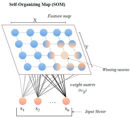
Figure 7.
The architecture of SOM.
The size of the weight vector ‘wi’ in SOM is controlled using the learning rate functions like the linear, the inverse of time, and the power series as given in Equations (30)–(32) [79].
where T represents the number of iterations and t is the order number of a certain it.
It is distinct from the other ANNs in the case of implementing the neighborhood function. A neighborhood function is a function that computes the rate of neighborhood change around the winner neuron in a neural network. Usually, the bubble and Gaussian functions (Equations (33) and (34)) are used as neighborhood functions in SOM.
where Nc = the index set of neighbor nodes close to the node with indices c, Rc, and Rij = indices of wc and wij, respectively, and ηcij = the neighborhood rank between nodes wc and wij.
6. Classification Techniques
The classification techniques are used to determine the category of new observations based on the training data. In the classification process, an algorithm first learns from the dataset or observations provided and then sorts each new observation into one of the classes. It enables us to divide enormous amounts of data into distinct classes. Various classification techniques that can be used for HRV features and can be executed in RapidMiner software are described below.
6.1. Generalized Linear Model
A generalized linear model is based on the global generalization of simple linear regression (GLM). Nelder and Wedderburn created it to consolidate a wide variety of statistical methods [80]. GLM consists of three elements, i.e., an error dispersal function, a linear forecaster, and an algorithm [81]. The probability distribution functions like Gaussian, binomial, and Poisson are used as the error distribution function. The linear predictor reveals the consistent impact sequence, and the technique delivers the best estimate of the design variables possible.
6.2. Naive Bayes
An example of a likelihood classifier, Naive Bayes (NB), is one that makes strong (naive) independent assertions across attributes and relies on Bayes’ theorem. With the class variable in place, it presumes that each attribute may be considered separately. If the fruit is red, round, and around 10 cm in diameter, we call it an apple. An NB technique would attribute equal weight to every parameter when calculating the chance that this item is an apple, irrespective of any correlations among color and sphericity or length. In numerous practical applications, the maximum likelihood method estimates parameters for the NB model (Figure 8). Despite its naïve design and simplistic assumptions, NB classifiers have performed well in various challenging real-world scenarios. Mathematically, the NB model can be expressed with the help of the discriminant function, as shown in Equation (35) [82].
where X = (x1, x2, …, xN) corresponds to the feature vector, ci indicates the class levels, P(ci) represents the prior likelihood, and P(xj|ci) denotes the restrictive likelihood.
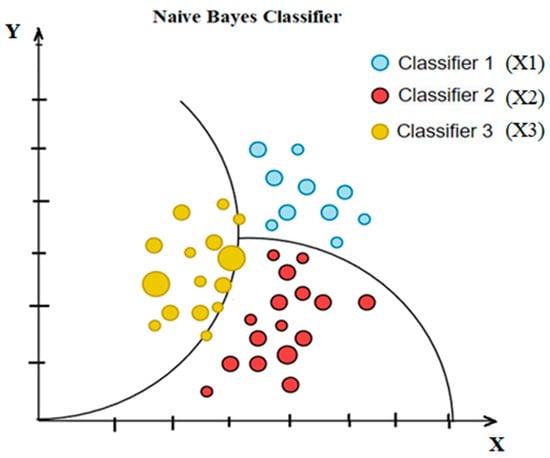
Figure 8.
Simple diagram of Naïve Bayes classifier.
6.3. Support Vector Machine
One standard supervised learning method, a support vector machine (SVM), may be used to address categorization and regression issues simultaneously. Its purpose is to find the ideal contour (called the hyperplane) for categorizing n-dimensional space into categories. The features in the dataset determine the dimension of the hyperplane. The SVM can be linear or non-linear based on the nature of the dataset. Data that can be split into two groups in a linear fashion are said to be differentiable, and the SVM classifier used in such cases is known as a linear SVM. A non-linear support vector machine can be employed if a linear classification scheme fails to work on a given dataset. A simple graphical representation of both the linear and non-linear SVM is presented in Figure 9 below.
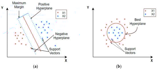
Figure 9.
Graphical representation of (a) linear and (b) non-linear support vector machines.
6.4. Logistic Regression
Logistic regression (LR) corresponds to a probabilistic statistical model widely used in classification problems. It aims at defining the connotation among a dichotomous dependent attribute and numerous independent attributes of the dataset [83]. The use of the logistic function f(z) (given with Equation (36)) mainly contributes to the wide acceptance of the LR classifier as its values always lie in the range of 0 to 1 [84]. In addition, the logistic function gives an attractive S-shaped representation of the cumulative outcome (z) of the independent attributes on the dependent attribute f(z) (Figure 10) [85]. It is clear from Figure 10 that the logistic regression is different from the linear regression in the case of its ability to limit the output in the range of 0 to 1.
where z is the cumulative effect of the independent variables, and f(z) is the dependent variable.
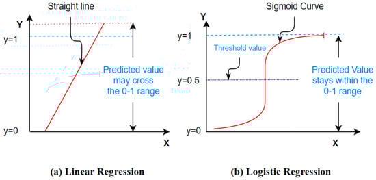
Figure 10.
A standard S–shaped illustration of the logistic function.
Equation (36) can be written as
Let us take .
where [p/(1 − p)] indicates the odds of the event occurring.
6.5. Deep Learning
Deep learning (DL) is a progressive unsupervised strategy for knowledge features or representations. It has created a novel tendency in ML and pattern identification [86,87]. The hypothetical foundation for DL is the notion of neural nets. DL models employ several hidden neurons and layers (often more than two) associated with conventional neural networks. In addition, the DL models incorporate advanced learning techniques, such as the autoencoder technique and restricted Boltzmann machine (RBM), which are not used in conventional neural networks [87]. A DL network enables automated attribute choosing by abstracting raw data at a high level. These networks can reveal hidden input attributes, enhancing classification performance [88]. Figure 11 displays the overall DL framework [73].
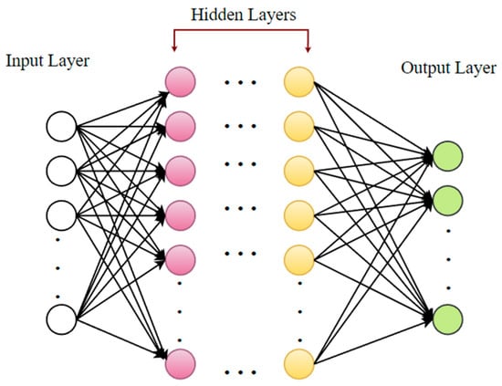
Figure 11.
A standard illustration of a deep neural network.
6.6. Decision Tree
The decision tree (DT) procedures are widespread categorization techniques in ML [89]. They separate the data recursively into two categories to construct a tree on the basis of its input attributes [82]. Various established mathematical procedures, such as an information gain, chi-square test, Ginni index, etc., are used to partition the data [89]. These methods provide the variables and threshold for subdividing the dataset input into distinct subgroups. The process of splitting is continued until a mature tree is created. A DT categorizer typically consists of internal nodes, divisions, and leaf nodes (Figure 12) [90]. The internal node represents a test on a feature, while the branches represent the test’s outcome and the leaf nodes denote class levels.
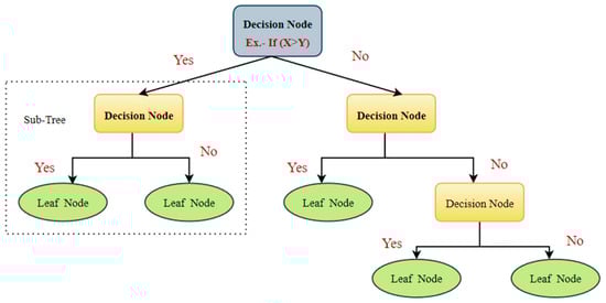
Figure 12.
A standard illustration of the DT classifier.
6.7. Random Forest (RF)
The RF model belongs to the composite classifications’ group of algorithms. It is useful for making predictions on the basis of the combination of a number of different decision trees [89]. All decision trees are produced using the portrayal of a subsection of the drilling subsets via replacing values or bagging. The concluding estimate is founded upon the most gained of the votes these decision trees give (Figure 13). The choice of two variables, specifically, the number of decision trees to be produced and the number of attributes to be nominated for budding the trees, shows a critical part in determining the efficiency of the RF architecture [91].
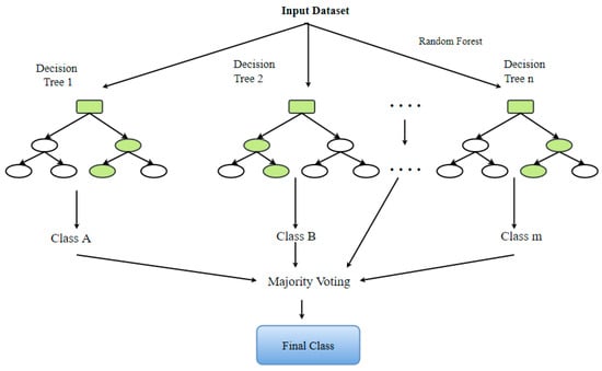
Figure 13.
The graphic illustration of a standard RF classifier.
6.8. Gradient Boosted Tree (GBT)
A gradient boosted tree (GBT) is an advanced decision tree approach that divides the dataset into subgroups using an optimization model like XGBoost. It is one of the popular models due to its capacity to deal with absent data and reduce the loss function [92]. It can determine the higher-order relationships between the input attributes [93] too. In each time step, the gradient-boosted tree builds a new tree to minimalize the residual of the existing system (Figure 14).
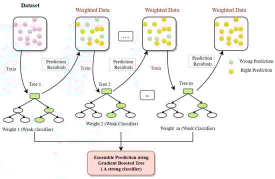
Figure 14.
The graphic depiction of an archetypal GBT classifier.
6.9. Fast Large Margin (FLM)
The FLM algorithm is a form of linear SVM. It originated from the fast-margin learner developed by Fan et al. (2008) [94]. This classifier yields similar results to traditional SVM and LR approaches. Nevertheless, the FLM classifier can deal with datasets, including millions of samples and attributes.
7. Applications of HRV Analysis
There are various applications of an HRV analysis. It has emerged as an important diagnostic tool in fields as diverse as cardiology, endocrinology, psychiatry, fetal monitoring, neonatal care, and many others. An HRV analysis can also help in understanding the effects of various external consumption factors, like alcohol, drugs, smoking, etc., on the pursuit of the autonomic nervous system. Some of the prominent applications are described in this section.
7.1. Diabetes Detection
Diabetes has emerged as one of the most common diseases worldwide. When blood sugar levels are not under control, the extra blood sugar builds up in the blood vessels and impacts how blood flows to different organs in the body. An inappropriate amount of secretion of insulin causes diabetes [94]. Primarily, two forms of diabetes exist.
Type 1 diabetes: If a person has type 1 diabetes, they need insulin injections or other treatments to receive enough insulin into the body. This is because the body loses the ability to make the right amount of insulin, which can cause high blood sugar levels and other health issues.
Type 2 diabetes: An individual with this form of diabetes does not need insulin and is not resistant to it. In this case, the body makes enough insulin, but it does not use that insulin for energy conversion. Since there is not enough energy, the body makes even more insulin, which causes the blood sugar to rise to abnormal levels [95].
Diabetes has been proven to be the leading cause of heart disease, renal malfunction, strokes, limb paralysis, and vision loss in individuals all over the globe. The majority of diabetes patients have other co-morbidities, such as obesity or hypertension. Diabetes has been linked to cholesterol, blocked arteries, myocardial infarction, and other serious consequences [96].
Recent studies reveal a strong link between HRV and glucose levels, indicating that diabetes causes gradual autonomic dysfunction and reduced heart rate variability [97]. A reduction in HRV features can indicate the potential of a volunteer being diabetic. Several studies attempt to develop viable solutions to the problem of diabetes detection based on an HRV analysis. Yildirim et al. (2019) proposed the automatic identification of diabetic patients by employing deep learning models on spectrogram images of RR intervals. The deep learning (DL) approach included pre-trained CNN models like DenseNet, AlexNet, ResNet, and VGGNet [98]. The spectrogram images were constructed utilizing the short-time Fourier transform (STFT) on the RR intervals. Among all the DL models, the DenseNet model presented an accuracy of 97.62% and a sensitivity of 100% for diagnosing diabetic patients. In another study, Rathod et al. (2021) analyzed the effect of type 2 diabetes mellitus (T2DM) on HRV features to determine the resultant autonomic dysfunction in diabetic patients [99]. The time-domain attributes (mean RRI and SDNN), frequency-domain features (total power, LF, and HF), and non-linear features (SD1 and SD2) were lower in diabetic patients than those of the control group in the resting state. When an orthostatic challenge was conducted as a stimulus to study the ANS reactivity, a blunted response of the ANS reactivity was exhibited by the T2DM patients. The authors then implemented the ML algorithms to detect autonomic dysfunction in T2DM patients. The Classification and Regression Tree (CART) model was able to identify the extent of autonomic dysfunction in individuals with TD2M with the highest accuracy of 84.04%. Thus, the authors recommended the use of HRV features in amalgamation with the CART model for the detection of autonomic dysfunction in TD2M patients. Table 1 lists some other papers issued in the last 5 years discussing the application of an HRV analysis in diabetes detection.

Table 1.
List of published papers in the last 5 years with novel approaches for diabetes detection based on HRV analysis.
7.2. Sleep Apnea Detection
Sleep is important for the proper functioning of the human body [109]. The brain passes through various stages of sleep as a person sleeps. They are mainly classified as rapid eye movement (REM) and non-rapid eye movement (NREM) [110]. Both of these phases are continually repeated during sleep [109]. When a person does not have typical cycles of REM and non-REM sleep, the body may face a variety of negative impacts, including weariness, a decrease in capacity to focus, disruptions in body metabolism, and other similar symptoms, even stroke [111]. Sleep apnea is one of the many diseases that disrupt these healthy sleeping cycles. It is a sleeping ailment categorized by recurrent starting and stopping of breathing while sleeping. Sleep apnea patients experience muscles at the back of their throats getting stretched and becoming more constricted, thus disrupting the normal breathing process [112]. This is a highly prevalent condition often observed more frequently in males than in women. Patients of any age can be affected by this ailment. However, middle-aged individuals are more likely to have it [113]. Sleep apnea can be treated if the patient is aware of the symptoms of sleep apnea, which reduces risk factors, and discusses future treatment options with their doctor [114]. Snoring and occasional breathing disruptions during sleep are the common symptoms of this disorder. Other indications include an abrupt awakening accompanied by shortness of breath, a headache upon waking, insomnia, focus issues, irritability, and hypersomnia. Sleep apnea has been related to various significant health problems such as diabetes, stroke, hypertension, obesity [115], and high blood pressure. Although this cannot be cured, it can be treated with various methods such as behavioral therapy, positive pressure therapy, oral breathing equipment, and even surgery [116,117]. Several pieces of research have been executed in the arena of sleep apnea diagnoses since an early diagnosis of the disease can reduce patient mortality. An HRV analysis has found several applications in the field of sleep, including assessing the severity of sleep apnea, categorizing sleep stages, and detecting sleep apnea events [118,119]. The consequence of disruptive sleep apnea (OSA) severity on HRV features was examined by Qin et al. (2021) [120]. The research was conducted on 1247 persons, among which 426 were healthy and 821 had OSA. The time-domain and non-linear HRV features exhibited less complexity and increased sympathetic dominance in OSA patients. Thus, the authors proposed an HRV analysis as a potential marker of cardiovascular activity in such patients. Recently, Nam et al. (2022) studied the relationship between the apnea–hypopnea index (AHI) and HRV in OSA patients. The authors analyzed the 24 h Holter monitoring-based HRV data and polysomnography data of 62 OSA patients. The results suggested that day/night VLF and LF ratios decreased with the increased severity of OSA. These features were also observed to associate independently with the AHI. Table 2 shows some HRV analysis research conducted for sleep apnea detection.
Table 2.
Studies conducted for sleep apnea diagnoses utilizing HRV analysis in the last 5 years.
7.3. Myocardial Infarction Detection
Myocardial infarction (MI) is a widespread illness known as a heart attack. The prevalence of heart attacks in India is 64.37 cases per 1000 individuals. According to a recent assessment, around 1.5 million myocardial infarctions occur annually in the United States (US) [1]. Myocardial infarction takes place when a segment or segments of the heart muscle are deprived of oxygen. This happens when there is a restriction in the blood supply to the heart’s muscles. The leading cause of MI is complete or partial artery blockage. Plaque deposits in coronary arteries can rupture and cause a blood clot. If the clot stops the arterial blood flow, the cardiac muscle will not receive enough blood, causing a heart attack. The risk factors for this cardiac issue have two aspects, i.e., genetic and acquired (from lifestyle, diseases, age, trauma, etc.) (Figure 15).
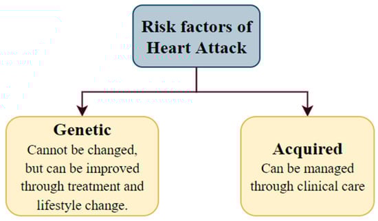
Figure 15.
The risk factors for heart attack.
The HRV features of patients who suffered from an acute myocardial infarction (AMI) are being analyzed extensively. According to most studies, patients with a decreased or abnormal HRV risk are dying within a few years of having an AMI. Many measures of HRV, including time-domain, spectral, and non-linear, have been employed in the risk stratification of post-AMI patients [126]. Sharma et al. (2019) proposed a model for accurately detecting heart failure utilizing decomposition-based attributes mined via HRV features. Three healthy volunteer datasets and two CHF datasets were used in the study. The Eigen Value Decomposition of the Hankel Matrix (EVDHM) technique was applied in this case for feature extraction. It employed least-square SVM with a radial basis function kernel as the classifier. The suggested approach produced an accuracy of 93.33%, a sensitivity of 91.41%, and a specificity of 94.90% utilizing 500 HRV samples [127]. Further, Shahnawaz et al. (2021) presented an ML model for automated uncovering of myocardial infarction founded on ultra-short-term HRV [128]. They used artificial neural networks (ANN), random forest, KNN, and SVM for categorization purposes and the Relu Activation Function to select and reduce features for the model. This model yielded an accuracy of 99.01% and a sensitivity of 100%.
7.4. Cardiac Arrhythmia Detection
A cardiac arrhythmia is when the heart beats erratically [129]. The primary reason for an arrhythmia can be a heart rate that is abnormally high, abnormally low, or irregular [130]. This happens due to abnormal signals from the heart. Mainly two kinds of heart arrhythmias exist. They are usually categorized using the heart rate, namely tachycardia and bradycardia (Figure 16) [131]. Tachycardia is a medical term used to describe an elevated heart rate that exceeds the normal range, often above 100 beats per minute in adult individuals. In contrast, bradycardia is characterized by a diminished heart rate, typically falling below 60 beats per minute among adult individuals. Both tachycardia and bradycardia can manifest within the context of sinus rhythm, wherein the heart’s electrical impulses originate from the sinus node, which serves as the heart’s intrinsic pacemaker. Various approaches to analyzing HRV signals may exhibit distinct behaviors when employed on individuals experiencing tachycardia or bradycardia as discussed below.
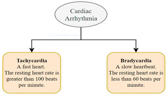
Figure 16.
Types of cardiac arrhythmias.
- Time-Domain Analysis:
In subjects with tachycardia, shorter RR intervals can result in reduced variability between consecutive intervals, potentially affecting time-domain measures such as the standard deviation of NN intervals (SDNN) and the root mean square of successive NN interval differences (RMSSD) [29].
In subjects with bradycardia, longer RR intervals might lead to increased variability, potentially influencing the same time-domain measures [132].
- Frequency-Domain Analysis:
In subjects with tachycardia, the faster heart rate can lead to higher-frequency power dominating the spectrum [133], potentially obscuring the interpretation of low-frequency (LF) and high-frequency (HF) components.
In subjects with bradycardia, the opposite might occur, making frequency-domain interpretation more straightforward [134].
- Non-linear Analysis:
Non-linear HRV analysis methods, such as Poincaré plots and fractal analyses, might be affected by the irregularity of the heart rate in tachycardia and the extended RR intervals in bradycardia [135]. These methods might need adjustments or specific considerations for accurate interpretation.
- Geometric Analysis:
Geometric methods, like the triangular index and Lorenz plot, might be sensitive to the distribution of RR intervals [136], which can differ in tachycardia and bradycardia. These methods might need normalization or transformation to account for such differences.
In general, the issues that might arise from arrhythmias include the risk of having a stroke and heart failure [137]. Arrhythmias have also been linked to a higher risk of blood clots. A blood clot can move from the heart to the brain and cause a stroke if it breaks away [138]. Many researchers have suggested different detection methods for cardiac arrhythmias. Atrial fibrillation (AF) is an arrhythmia that may modify heart rhythm dynamics and ECG morphology. It is distinguished by the presence of irregular and rapid electrical impulses inside the atria, resulting in an irregular and frequently elevated heart rate. The measurement of HRV in individuals diagnosed with AF might offer valuable insights into the impact of the autonomic nervous system on the development and progression of this condition. Furthermore, such an analysis may have significant consequences for the process of assessing an individual’s risk level and managing their treatment plan. Nevertheless, it is crucial to acknowledge that the study of HRV in patients with AF can present challenges owing to the irregularity of the cardiac rhythm. Conventional approaches for measuring HRV may not be well-suited for examining datasets characterized by irregular intervals between successive heartbeats. Various algorithms and methodologies have been specifically designed to tackle these challenges and derive significant metrics related to HRV from the data of individuals with AF.
The examination of HRV in patients with AF has the potential to provide significant insights into the role of the autonomic nervous system in the development of the arrhythmia, as well as its potential for predicting unfavorable outcomes or informing treatment strategies. However, it is imperative to use caution when interpreting the findings and to consider them in connection with other clinical and diagnostic factors. Relying just on an HRV analysis may not yield a thorough understanding of a patient’s cardiac well-being. A study by Christov et al. (2018) ranked HRV features for atrial fibrillation detection [139]. They found that the PNN50, SD1/SD2, and RR mean are the three top ranked HRV features, as well as the full set of HRV features achieving a 13%-point higher arrhythmia detection performance compared to the set of beat morphology features. Other recent studies for arrhythmia detection with an HRV analysis can be found in [140,141,142,143]. The experimental results revealed that the HRV descriptors are effective measures for AF identification. In another study, Singh et al. (2019) proposed an arrhythmia detection technique using a time–frequency (T-F) analysis of HRV features [144]. The back-propagation neural networks, in combination with three different types of decision rules, were employed to achieve the classification accuracy of 95.98% for the low-frequency (LF) band and 97.13% for the high-frequency (HF) band [144]. A study by Ahmed et al. (2022) highlighted the development of a client–server paradigm for analyzing HRV features to detect arrhythmias [145]. The proposed platform performed all the real-time steps, from feature extraction to classification. Smoothed Pseudo Wigner–Ville Distribution (SPWVD) was used for the HRV analysis, and SVM was used as the classifier to achieve a classification accuracy up to 97.82%. The classification result can be further sent to clinicians for an interpretation and diagnosis.
7.5. Blood Pressure/Hypertension Detection
Blood pressure (BP) refers to the force of pumping blood against the walls of the arteries. The condition is called hypertension when this pressure is too high [146]. Two numbers are used to express someone’s blood pressure. The first number, the systolic pressure, indicates the pressure in the blood arteries whenever the heart beats or contracts. The second number, the diastolic pressure, indicates the pressure in the blood vessels while the heart rests between the beats [147]. If the systolic BP and the diastolic BP are ≥140 mmHg and ≥90 mmHg, respectively, on two separate days, the patient is said to be suffering from hypertension [148]. Numerous structural and functional alterations of the cardiac muscles are induced in individuals with hypertension due to more workload on the heart. These alterations might increase the cardiovascular risk of hypertensive persons over and above the danger caused by an increase in blood pressure on its own. In recent years, many researchers have studied the feasibility of an HRV analysis as a marker for hypertension detection [149]. In a study by Lan et al. (2018), it was shown that an HRV analysis can predict hypertension at an early stage [150]. The study used 3 months of PPG-based HRV statistics from hypertensive and non-hypertensive participants to calculate HRV features. Six HRV features were utilized in data mining to predict hypertension. It was found that the SDNN feature had the best predictive potential with an accuracy of 85.47%. In light of the findings, the researchers recommended that the PPG-based HRV statistics composed via the wearable devices can be a potential candidate for hypertension prediction with acceptable accuracy. An HRV analysis was tested as a prognostic tool for identifying high-risk patients suffering from hypertension by Deka et al. (2021) [151]. Their study used a hybrid method founded on the dual-tree complex wavelet packet transform (DTCWPT) and other time-domain and non-linear HRV analysis methods to extract features. These features were then fed to the cost-sensitive RUSBoost algorithm, which produced a G-mean and F1 score of 0.9352 and 0.9347, respectively. Table 3 shows selected recent articles on an HRV analysis for hypertension detection.
Table 3.
List of published papers in recent years that have used HRV analysis methods for the detection of hypertension.
7.6. Detection of Renal Failure
An HRV analysis is a valuable tool for assessing autonomic dysfunction, which is vital in predicting the cardiovascular morbidity and mortality associated with kidney failure patients [156]. HRV indices have been analyzed [157] by researchers on individuals diagnosed with renal failure. The association between HRV features and the concentrations of electrolyte ions before and after dialysis was presented in a paper by Tsai et al. (2002) [158]. The HRV features from 5 min ECG signals of twenty patients with chronic kidney failure (CRF) were evaluated. After hemodialysis, the study showed calcium negatively correlated with the average RR intervals and the normalized HF power. Chou et al. (2019) investigated the diagnostic importance of HRV on renal function in kidney failure patients [156]. The authors involved 326 non-dialysis chronic kidney disease (CKD) patients in experimental research of 2.02 years, and their HRV features were analyzed regularly. It was found that the values of HRV features became reduced with the increased severity of CKD. The computation of LF/HF divulged useful information on the progress of CKD apart from the other risk factors. Some more recent articles on the application of HRV features in renal failure are summarized in Table 4.
Table 4.
List of published papers in recent years that have used novel HRV analysis methods for the detection of renal failure.
7.7. Psychiatric Disorder Detection
The dynamic regulation of the heart can be significantly affected by psychological emotions and activities [162,163]. Hence, people with psychiatric problems are at risk of developing cardiovascular diseases [164]. Multiple symptoms of mental disorders are also associated with the disruption of ANS. For instance, depressed people frequently have dry mouth, constipation/diarrhea, and sleeplessness. In the last few decades, many researchers have examined the feasibility of an HRV analysis to elucidate the physiology of psychiatric diseases and their relation to the cardiovascular system [165].
A study by Carney et al. (2001) found that patients with depression and cardiovascular conditions have lower short- and long-term HRV feature values [166]. Other usual mental ailments, such as anxiety disorders, frequently coexist with ANS disorders because of their close relationship. An analysis of HRV data was used in a work by Miu et al. (2009) to understand the relationship between anxiety and malfunction in the ANS [167]. It has been shown that several antipsychotic medications can harm the functioning of the ANS. In particular, ANS dysfunction and abnormal cardiac repolarizations are detected in people medicated with the antipsychotic drug clozapine [168]. These findings point to the possibility that both the schizophrenia disease and the medication prescribed for its therapy could add to the increased likelihood of coronary sickness. Patients who are untreated for their schizophrenia exhibit a reduction in HRV feature values like RMSSD, pNN50, and high-frequency spectral power compared to healthy controls, suggesting a decreased vagal modulation [168]. Some more papers on the application of an HRV analysis in psychiatric disorders are discussed in Table 5.
Table 5.
Recent published papers on the application of HRV analysis in psychiatric disorders.
7.8. Monitoring of Fetal Distress and Neonatal Critical Care
Fetal inspection is vital and must precisely mirror embryonic well-being, identify the most plausible development process, and correctly envisage critical perinatal consequences. Thus, the primary goal of fetal monitoring is to offer precise and efficient care units for an early diagnosis of the onset of potentially life-threatening diseases. The fetus’s ability to survive, thrive, and progress into the neonatal stage depends on proper blood pressure, volume, and fluid dynamics. Prenatal cardiovascular control disturbances can increase fetal and neonatal mortality and morbidity.
Neonatal care is equally important to avoid unintentional complications. Patients in a Neonatal Intensive Treatment Unit (NICU) require specialized assistance, the efficiency of which is heavily reliant on the functioning of the medical equipment. The development of surveillance and imaging techniques improves predictive tactics and aids in preventing some complications. An HRV analysis has considerably aided neonatal care in neonatal sepsis detection, neonatal necrotizing enterocolitis monitoring, predicting preterm birth, avoiding possible complications, etc. For example, Kasai et al. (2019) examined the changes in HRV as a potential marker of the time and severity of acute hypoxia–ischemia (HI) [176]. The authors created umbilical cord occlusion of chronically instrumented fetal sheep to simulate HI and monitored the HR and HRV features for 72 h. It was found that the HI groups exhibited lower VLF power and increased sample entropy in the initial 3 h. Also, the spectral power change towards a higher frequency band was observed, suggesting autonomic dysfunction after HI. According to the findings, the authors of the study proposed that the changes in HR patterns can have predictive usage in the initial hours of HI onset. In a study by Joshi et al. (2020), the prognostic capability of HRV features, respiratory factors, and ECG-derived estimates of infant motion to predict neonatal sepsis were examined [177]. A total of 22 features were extracted, and an NB classifier was employed to differentiate between the control and septic states. The efficiency of the proposed system was analyzed utilizing the region underneath the receiver functioning feature (AUROC) curve and the true positive rate (TPR). When the time of sepsis came closer, HRV demonstrated massive decelerations. Moreover, it was observed that the HR could not be increased in response to pathological HR slowing down. On the basis of the outcomes, the writers recommended that the projected technique can be utilized as an early indicator of sepsis.
7.9. Grasping the Idea of the Impact of Alcohol on ANS Activity
Consuming excessive alcohol is related to an augmented hazard of sickness and death [178]. It is a global health problem, which is required to be dealt with as soon as possible. A rise in blood pressure, arrhythmias (most notably atrial fibrillation), liver cirrhosis, a hemorrhagic blow, wounds, and malignancies of the liver, colorectum, breast, and upper digestive tract have been linked to alcohol consumption [179,180]. Alcohol use over a prolonged period has been shown to have adverse effects on numerous body parts and structures, most notably the neurological system. The strong connection that exists between the ANS and the cardiovascular system (CV) is one of the primary issues that donate to the elevated risk of a cardiovascular ailment (CVD) in alcoholics [181]. The study of an HRV analysis can provide a non-invasive estimate of the imbalance in ANS physiology and determine the level of cardiovascular danger posed with various clinical conditions. Hence, many HRV analysis experiments have been executed to understand the consequence of alcohol consumption on the ANS. In a study by Pop et al. (2021), the authors examined the 5 min HRV features of volunteers in the supine position, and the time and frequency domain HRV attributes were extracted [182]. According to their findings, binge drinkers and casual drinkers exhibited a minor alteration in the frequency domain HRV features. On the other hand, heavy drinkers had considerably lower values of time-domain HRV features (SDNN and RMSSD) and HF components. Further, the heavy drinkers had a higher LF/HF value, suggesting parasympathetic inhibition [182]. The GBT regression model revealed that age and alcohol intake had the highest impact on the HRV features. In the same year, Brunner et al. (2021) also analyzed the effect of alcohol intake on cardiac autonomic regulation [183]. Fifteen volunteers participated in the study, where an HRV signal analysis was executed before, during, and after alcohol consumption. It was found that the values of HRV features were decreased, and mean HR was increased upon alcohol consumption. On the basis of the outcomes, the authors suggested that alcohol consumption induced sympathetic dominance and a decrease in parasympathetic activity, causing autonomic imbalance.
7.10. ANS Activity of Patients Undergoing Weaning from Mechanical Ventilation
The analysis of HRV can be conducted using two separate domains: time and frequency. Each domain offers distinct insights into the cardiac function, including the potential of certain HRV features in the time and frequency domains to predict the readiness of mechanically ventilated patients for extubation. The determination of extubation readiness pertains to a patient’s capacity to respire autonomously without reliance on mechanical support, and it represents a pivotal judgment within the context of the intensive care setting. Various HRV properties can be derived from ECG signals obtained from individuals who have had a spontaneous breathing trial (SBT), which is a test conducted to evaluate their preparedness for extubation. The utilization of HRV properties can assist in the classification of patients into distinct groups, namely successful or failed extubation groups.
A significant observation was made regarding a reduction in HRV features during the transition from PSV to the spontaneous breathing trial (SBT). This decrease was shown to be significant in the unsuccessful category but not in the winning category [184]. The utilization of mechanical ventilator assistance and the process of transitioning to spontaneous breathing, also known as weaning, results in notable changes in alveolar and intrathoracic pressure. These variations have a direct impact on thoracic blood volume and flow. Compensatory adjustments in the autonomic tone take place in order to maintain a sufficient delivery of oxygen to tissues. However, these autonomic reactions might lead to cardiovascular dysfunction, ultimately resulting in the failure of weaning. Approximately 66% of the patients in a study of Frazier et al. (2008) exhibited a typical autonomic function, with greater severity of dysfunction observed in individuals who were not able to maintain breathing on their own [185]. In their study, Krasteva et al. (2018) explored three fundamental strategies to ensure an appropriate autonomic cardiac control reaction during the weaning phase of cardio-respiratory stress in patients. The group model that achieved effectiveness had a decrease in overall activity accompanied by a rise in sympathetic tone and a decrease in vagal tone. The latter correlated with both the respiration rate and tidal volume. Deviations from the established HRV model serve as indicators for the occurrence of weaning failure, with a precision of 92.6% for pressure support ventilation, 81.5% for spontaneous breathing trials (SBT), and 96.3% for the combination of SBT and PSV [186]. Patients who experienced failure in the process of weaning revealed a notable drop in the RR sample entropy, LF, HF, and α1 exponent in comparison to participants who successfully underwent weaning. The alterations seen in the two phases exhibited contrasting trends, with the exception of the Mean Squared Error (MSE), which showed an upsurge within as well as between the groups. Hence, Vassilios E. et al. (2011) proposed that the application of a non-linear analysis to cardio-respiratory dynamics has the potential to enhance the predictive value of weaning efficacy in patients undergoing surgery [187].
8. Conclusions
An HRV analysis has emerged as a valuable diagnostic tool in the last few decades, having a wide variety of applications [188]. In this study, various methods of HRV feature generation were discussed. The extraction of relevant features performs a significant part in deciding the prediction capability of the HRV signal-based diagnostic approach. Hence, a description of popular HRV feature extraction methods was provided. The performance of ML-based classifiers strongly depends on selecting relevant features with distinguishing capabilities. Therefore, several feature ranking methods on the basis of weights and feature dimensionality reduction approaches were discussed. The important classifiers utilized by scholars in the case of the categorization of HRV features were described. Finally, various clinical applications of an HRV analysis were summarized. The information gathered in this article will help future researchers to obtain comprehensive knowledge about the recent trends in HRV analyses and their prospective applications.
Author Contributions
Conceptualization, S.K.N. and K.P.; methodology, S.K.N., B.P. and B.M.; software, S.K.N., J.S. and S.S.R.; validation, S.K.N., B.P. and K.P.; formal analysis, M.J.; investigation, S.K.N.; resources, K.P., S.S.R. and J.S.; data curation, S.K.N.; writing—original draft preparation, S.K.N., K.P., M.J. and J.W.; writing—review and editing, M.J. and J.W.; visualization, S.K.N.; supervision, K.P. All authors have read and agreed to the published version of the manuscript.
Funding
This research received no external funding.
Data Availability Statement
Not applicable.
Conflicts of Interest
The authors declare no conflict of interest.
Sample Availability
Not applicable.
References
- Rajendra Acharya, U.; Paul Joseph, K.; Kannathal, N.; Lim, C.M.; Suri, J.S. Heart Rate Variability: A review. Med. Biol. Eng. Comput. 2006, 44, 1031–1051. [Google Scholar] [CrossRef]
- Kim, H.G.; Cheon, E.J.; Bai, D.S.; Lee, Y.H.; Koo, B.H. Stress and heart rate variability: A meta-analysis and review of the literature. Psychiatry Investig. 2018, 15, 235. [Google Scholar] [CrossRef] [PubMed]
- Saul, J.P. Beat-to-beat variations of heart rate reflect modulation of cardiac autonomic outflow. Physiology 1990, 5, 32–37. [Google Scholar] [CrossRef]
- Levy, M.N.; Schwartz, P.J. Vagal Control of the Heart: Experimental Basis and Clinical Implications; Futura Pub. Co.: Austin, TX, USA, 1994. [Google Scholar]
- Schwartz, P.J. Sympathetic nervous system and cardiac arrhythmias. Card. Electrophysiol. 1990, 330–343. [Google Scholar]
- Camm, A.J.; Malik, M.; Bigger, J.T.; Breithardt, G.; Cerutti, S.; Cohen, R.J.; Coumel, P.; Fallen, E.L.; Kennedy, H.L.; Kleiger, R.E. Heart rate variability: Standards of measurement, physiological interpretation and clinical use. Task Force of the European Society of Cardiology and the North American Society of Pacing and Electrophysiology. Circulation 1996, 93, 1043–1065. [Google Scholar]
- Ge, D.; Srinivasan, N.; Krishnan, S.M. Cardiac arrhythmia classification using autoregressive modeling. Biomed. Eng. Online 2002, 1, 5. [Google Scholar] [CrossRef]
- Rosenstein, M.T.; Collins, J.J.; De Luca, C.J. A practical method for calculating largest Lyapunov exponents from small data sets. Phys. D Nonlinear Phenom. 1993, 65, 117–134. [Google Scholar] [CrossRef]
- Pincus, S.M. Approximate entropy as a measure of system complexity. Proc. Nat. Acad. Sci. USA 1991, 88, 2297–2301. [Google Scholar] [CrossRef] [PubMed]
- Peng, C.-K.; Havlin, S.; Hausdorff, J.; Mietus, J.; Stanley, H.; Goldberger, A. Fractal mechanisms and heart rate dynamics: Long-range correlations and their breakdown with disease. J. Electrocardiol. 1995, 28, 59–65. [Google Scholar] [CrossRef]
- Burlacu, A.; Brinza, C.; Brezulianu, A.; Covic, A. Accurate and early detection of sleepiness, fatigue and stress levels in drivers through Heart Rate Variability parameters: A systematic review. Rev. Cardiovasc. Med. 2021, 22, 845–852. [Google Scholar] [CrossRef] [PubMed]
- Ishaque, S.; Khan, N.; Krishnan, S. Trends in heart-rate variability signal analysis. Front. Digit. Health 2021, 3, 639444. [Google Scholar] [CrossRef] [PubMed]
- Jaderberg, M.; Vedaldi, A.; Zisserman, A. Deep features for text spotting. In Proceedings of the Computer Vision–ECCV 2014: 13th European Conference, Zurich, Switzerland, 6–12 September 2014; Proceedings, Part IV 13. Springer International Publishing: Berlin/Heidelberg, Germany, 2014; pp. 512–528. [Google Scholar]
- Lascu, M.; Lascu, D. LabVIEW event detection using Pan-Tompkins algorithm. In Proceedings of the 7th WSEAS International Conference on Signal, Speech and Image Processing, Beijing, China, 15–17 September 2007. [Google Scholar]
- Sharma, A.; Patidar, S.; Upadhyay, A.; Acharya, U.R. Accurate tunable-Q wavelet transform based method for QRS complex detection. Comput. Electr. Eng. 2019, 75, 101–111. [Google Scholar] [CrossRef]
- Wehler, D.; Jelinek, H.F.; Gronau, A.; Wessel, N.; Kraemer, J.F.; Krones, R.; Penzel, T. Reliability of heart-rate-variability features derived from ultra-short ECG recordings and their validity in the assessment of cardiac autonomic neuropathy. Biomed. Signal Process. Control 2021, 68, 102651. [Google Scholar] [CrossRef]
- Liu, F.; Wei, S.; Lin, F.; Jiang, X.; Liu, C. An overview of signal quality indices on dynamic ECG signal quality assessment. In Feature Engineering and Computational Intelligence in ECG Monitoring; Liu, C., Li, J., Eds.; Springer: Singapore, 2020; pp. 33–54. [Google Scholar]
- Clifford, G.D.; Moody, G.B. Signal quality in cardiorespiratory monitoring. Physiol. Meas. 2012, 33, E01. [Google Scholar] [CrossRef]
- Swai, J.; Hu, Z.; Zhao, X.; Rugambwa, T.; Ming, G. Heart rate and heart rate variability comparison between postural orthostatic tachycardia syndrome versus healthy participants; a systematic review and meta-analysis. BMC Cardiovasc. Disord. 2019, 19, 320. [Google Scholar] [CrossRef] [PubMed]
- Chou, E.-F.; Khine, M.; Lockhart, T.; Soangra, R. Effects of ecg data length on heart rate variability among young healthy adults. Sensors 2021, 21, 6286. [Google Scholar] [CrossRef]
- Chen, Y.-S.; Lu, W.-A.; Pagaduan, J.C.; Kuo, C.-D. A novel smartphone app for the measurement of ultra–short-term and short-term heart rate variability: Validity and reliability study. JMIR Mhealth Uhealth 2020, 8, e18761. [Google Scholar] [CrossRef]
- Taoum, A.; Bisiaux, A.; Tilquin, F.; Le Guillou, Y.; Carrault, G. Validity of Ultra-Short-Term HRV Analysis Using PPG—A Preliminary Study. Sensors 2022, 22, 7995. [Google Scholar] [CrossRef] [PubMed]
- Burma, J.S.; Graver, S.; Miutz, L.N.; Macaulay, A.; Copeland, P.V.; Smirl, J.D. The validity and reliability of ultra-short-term heart rate variability parameters and the influence of physiological covariates. J. Appl. Physiol. 2021, 130, 1848–1867. [Google Scholar] [CrossRef]
- Shaffer, F.; Ginsberg, J. An overview of heart rate variability metrics and norms. Front. Public Health 2017, 5, 258. [Google Scholar] [CrossRef]
- Nardelli, M.; Greco, A.; Bianchi, M.; Scilingo, E.P.; Valenza, G. Classifying affective haptic stimuli through gender-specific heart rate variability nonlinear analysis. IEEE Trans. Affect. Comput. 2018, 11, 459–469. [Google Scholar] [CrossRef]
- Cepeda, F.X.; Lapointe, M.; Tan, C.O.; Taylor, J.A. Inconsistent relation of nonlinear heart rate variability indices to increasing vagal tone in healthy humans. Auton. Neurosci. 2018, 213, 1–7. [Google Scholar] [CrossRef] [PubMed]
- Hoshi, R.A.; Andreão, R.V.; Santos, I.S.; Dantas, E.M.; Mill, J.G.; Lotufo, P.A.; Bensenor, I.M. Linear and nonlinear analyses of heart rate variability following sorthostatism in subclinical hypothyroidism. Medicine 2019, 98, e14140. [Google Scholar] [CrossRef]
- Cartas-Rosado, R.; Becerra-Luna, B.; Martinez-Memije, R.; Infante-Vazquez, O.; Lerma, C.; Perez-Grovas, H.; Rodríguez-Chagolla, J.M. Continuous wavelet transform based processing for estimating the power spectrum content of heart rate variability during hemodiafiltration. Biomed. Signal Process. Control 2020, 62, 102031. [Google Scholar] [CrossRef]
- Kleiger, R.E.; Stein, P.K.; Bigger, J.T., Jr. Heart rate variability: Measurement and clinical utility. Ann. Noninvasive Electrocardiol. 2005, 10, 88–101. [Google Scholar] [CrossRef]
- Tarvainen, M.P.; Lipponen, J.A.; Kuoppa, P. Analysis and Preprocessing of HRV—Kubios HRV Software. In ECG Time Series Variability Analysis: Engineering and Medicine; CRC Press: Boca Raton, FL, USA, 2017; pp. 159–186. [Google Scholar]
- Nagendra, H.; Kumar, V.; Mukherjee, S. Cognitive Behavior Evaluation Based on Physiological Parameters among Young Healthy Subjects with Yoga as Intervention. Comput. Math. Methods Med. 2015, 2015, 821061. [Google Scholar] [CrossRef]
- Marina Medina, C.; Blanca de la Cruz, T.; Alberto Garrido, E.; Marco Antonio Garrido, S.; José, N.O. Normal values of heart rate variability at rest in a young, healthy and active Mexican population. Health 2012, 4, 720–726. [Google Scholar]
- Tarvainen, M.P.; Niskanen, J.P.; Lipponen, J.A.; Ranta-Aho, P.O.; Karjalainen, P.A. Kubios HRV–heart rate variability analysis software. Comput. Methods Programs Biomed. 2014, 113, 210–220. [Google Scholar] [CrossRef]
- Peng, C.K.; Havlin, S.; Stanley, H.E.; Goldberger, A.L. Quantification of scaling exponents and crossover phenomena in nonstationary heartbeat time series. Chaos Interdiscip. J. Nonlinear Sci. 1995, 5, 82–87. [Google Scholar] [CrossRef]
- Wessel, N.; Marwan, N.; Meyerfeldt, U.; Schirdewan, A.; Kurths, J. Recurrence quantification analysis to characterise the heart rate variability before the onset of ventricular tachycardia. In Medical Data Analysis, Proceedings of the Second International Symposium, ISMDA 2001 Madrid, Spain, 8–9 October 2001; Proceedings 2; Springer: Berlin/Heidelberg, Germany, 2001; pp. 295–301. [Google Scholar]
- Marwan, N.; Romano, M.C.; Thiel, M.; Kurths, J. Recurrence plots for the analysis of complex systems. Phys. Rep. 2007, 438, 237–329. [Google Scholar] [CrossRef]
- Nayak, S.K.; Bit, A.; Dey, A.; Mohapatra, B.; Pal, K. A review on the nonlinear dynamical system analysis of electrocardiogram signal. J. Healthc. Eng. 2018, 2018, 6920420. [Google Scholar] [CrossRef]
- Eckmann, J.-P.; Kamphorst, S.O.; Ruelle, D. Recurrence plots of dynamical systems. World Sci. Ser. Nonlinear Sci. Ser. A 1995, 16, 441–446. [Google Scholar]
- Martín-González, S.; Navarro-Mesa, J.L.; Juliá-Serdá, G.; Ramírez-Ávila, G.M.; Ravelo-García, A.G. Improving the understanding of sleep apnea characterization using Recurrence Quantification Analysis by defining overall acceptable values for the dimensionality of the system, the delay, and the distance threshold. PLoS ONE 2018, 13, e0194462. [Google Scholar] [CrossRef]
- Webber, C.L., Jr.; Marwan, N. Recurrence quantification analysis. In Theory and Best Practices; Springer: Berlin/Heidelberg, Germany, 2015; p. 426. [Google Scholar]
- Yang, H. Multiscale Recurrence Quantification Analysis of Spatial Cardiac Vectorcardiogram Signals. IEEE Trans. Biomed. Eng. 2010, 58, 339–347. [Google Scholar] [CrossRef] [PubMed]
- Sharma, V. Deterministic Chaos and Fractal Complexity in the Dynamics of Cardiovascular Behavior: Perspectives on a New Frontier. Open Cardiovasc. Med. J. 2009, 3, 110–123. [Google Scholar] [CrossRef] [PubMed]
- Karavaev, A.S.; Ishbulatov, Y.M.; Ponomarenko, V.I.; Bezruchko, B.P.; Kiselev, A.R.; Prokhorov, M.D. Autonomic control is a source of dynamical chaos in the cardiovascular system. Chaos Interdiscip. J. Nonlinear Sci. 2019, 29, 121101. [Google Scholar] [CrossRef] [PubMed]
- Huang, N.E.; Shen, Z.; Long, S.R.; Wu, M.C.; Shih, H.H.; Zheng, Q.; Yen, N.-C.; Tung, C.C.; Liu, H.H. The empirical mode decomposition and the Hilbert spectrum for nonlinear and non-stationary time series analysis. Proc. R. Soc. London. Ser. A Math. Phys. Eng. Sci. 1998, 454, 903–995. [Google Scholar] [CrossRef]
- Bajaj, V.; Pachori, R.B. Classification of Seizure and Nonseizure EEG Signals Using Empirical Mode Decomposition. IEEE Trans. Inf. Technol. Biomed. 2011, 16, 1135–1142. [Google Scholar] [CrossRef]
- Acharya, U.R.; Fujita, H.; Sudarshan, V.K.; Oh, S.L.; Muhammad, A.; Koh, J.E.; Tan, J.H.; Chua, C.K.; Chua, K.P.; San Tan, R. Application of empirical mode decomposition (EMD) for automated identification of congestive heart failure using heart rate signals. Neural Comput. Appl. 2017, 28, 3073–3094. [Google Scholar] [CrossRef]
- Chen, M.; He, A.; Feng, K.; Liu, G.; Wang, Q.J.E. Empirical mode decomposition as a novel approach to study heart rate variability in congestive heart failure assessment. Entropy 2019, 21, 1169. [Google Scholar] [CrossRef]
- Acharya, U.R.; Vidya, K.S.; Ghista, D.N.; Lim WJ, E.; Molinari, F.; Sankaranarayanan, M. Computer-aided diagnosis of diabetic subjects by heart rate variability signals using discrete wavelet transform method. Knowl.-Based Syst. 2015, 81, 56–64. [Google Scholar] [CrossRef]
- Hei, Y.; Yuan, T.; Fan, Z.; Yang, B.; Hu, J. Sleep staging classification based on a new parallel fusion method of multiple sources signals. Physiol. Meas. 2022, 43, 045003. [Google Scholar] [CrossRef]
- Hu, Q.; Qin, A.; Zhang, Q.; He, J.; Sun, G. Fault diagnosis based on weighted extreme learning machine with wavelet packet decomposition and KPCA. IEEE Sens. J. 2018, 18, 8472–8483. [Google Scholar] [CrossRef]
- Addison, P.S. The Illustrated Wavelet Transform Handbook: Introductory Theory and Applications in Science, Engineering, Medicine and Finance; CRC Press: Boca Raton, FL, USA, 2002. [Google Scholar]
- Geng, D.Y.; Zhao, J.; Wang, C.X.; Ning, Q. A decision support system for automatic sleep staging from HRV using wavelet packet decomposition and energy features. Biomed. Signal Process. Control 2020, 56, 101722. [Google Scholar] [CrossRef]
- Hossen, A.; Qasim, S. Identification of obstructive sleep apnea using artificial neural networks and wavelet packet decomposition of the HRV signal. J. Eng. Res. 2020, 17, 24–33. [Google Scholar] [CrossRef]
- Akar, S.A.; Kara, S.; Bilgic, V. Investigation of heart rate variability in major depression patients using wavelet packet transform. Psychiatry Res. 2016, 238, 326–332. [Google Scholar] [CrossRef] [PubMed]
- Wang, F.; Wang, P.; Zhang, X.; Li, H.; Himed, B. An overview of parametric modeling and methods for radar target detection with limited data. IEEE Access 2021, 9, 60459–60469. [Google Scholar] [CrossRef]
- Faal, M.; Almasganj, F. ECG Signal Modeling Using Volatility Properties: Its Application in Sleep Apnea Syndrome. J. Healthc. Eng. 2021, 2021, 4894501. [Google Scholar] [CrossRef]
- Pande, K.; Subhadarshini, S.; Gaur, D.; Nayak, S.K.; Pal, K. Analysis of ECG Signals to Investigate the Effect of a Humorous Audio-Visual Stimulus on Autonomic Nervous System and Heart of Females. In Design and Development of Affordable Healthcare Technologies; IGI Global: Hershey, PA, USA, 2018; pp. 239–256. [Google Scholar]
- Nayak, S.K.; Pradhan, B.K.; Banerjee, I.; Pal, K. Analysis of heart rate variability to understand the effect of cannabis consumption on Indian male paddy-field workers. Biomed. Signal Process. Control 2020, 62, 102072. [Google Scholar] [CrossRef]
- Lei, S. A feature selection method based on information gain and genetic algorithm. In Proceedings of the 2012 International Conference on Computer Science and Electronics Engineering, Hangzhou, China, 23–25 March 2012; IEEE: New York, NY, USA, 2012; Volume 2, pp. 355–358. [Google Scholar]
- Dragomir, S.S.; Goh, C.J. A counterpart of Jensen’s discrete inequality for differentiable convex mappings and applications in information theory. Math. Comput. Model. 1996, 24, 1–11. [Google Scholar] [CrossRef]
- Priyadarsini, R.P.; Valarmathi, M.L.; Sivakumari, S. Gain ratio based feature selection method for privacy preservation. ICTACT J. Soft Comput. 2011, 1, 201–205. [Google Scholar]
- Kendall, A.; Gal, Y. What uncertainties do we need in bayesian deep learning for computer vision? Adv. Neural Inf. Process. Syst. 2017, 30. [Google Scholar]
- Wu, L.; Wang, Y.; Zhang, S.; Zhang, Y. Fusing gini index and term frequency for text feature selection. In Proceedings of the 2017 IEEE Third International Conference on Multimedia Big Data (BigMM), Laguna Hills, CA, USA, 19–21 April 2017; IEEE: New York, NY, USA, 2017; pp. 280–283. [Google Scholar]
- Perveen, N.; Gupta, S.; Verma, K. Facial expression recognition using facial characteristic points and Gini index. In Proceedings of the 2012 Students Conference on Engineering and Systems, Allahabad, India, 16–18 March 2012; IEEE: New York, NY, USA, 2012; pp. 1–6. [Google Scholar]
- Wu, R. Improved K-Modes Clustering Method Based on Chi-square Statistics. In Proceedings of the 2010 IEEE International Conference on Granular Computing, San Jose, CA, USA, 14–16 August 2010; IEEE: New York, NY, USA, 2010; pp. 808–811. [Google Scholar]
- Wang, S.E.N.; Zhang, L.I. A supervised correlation coefficient method: Detection of different correlation. In Proceedings of the 2020 12th International Conference on Advanced Computational Intelligence (ICACI), Dali, China, 14–16 March 2020; IEEE: New York, NY, USA, 2020; pp. 408–411. [Google Scholar]
- Altman, D.G.; Bland, J.M. Standard deviations and standard errors. BMJ 2005, 331, 903. [Google Scholar] [CrossRef] [PubMed]
- Urbanowicz, R.J.; Meeker, M.; La Cava, W.; Olson, R.S.; Moore, J.H. Relief-based feature selection: Introduction and review. J. Biomed. Inform. 2018, 85, 189–203. [Google Scholar] [CrossRef]
- Zhang, Y. Support vector machine classification algorithm and its application. In Information Computing and Applications, Proceedings of the Third International Conference, ICICA 2012, Chengde, China, 14–16 September 2012; Proceedings, Part II 3; Springer Berlin Heidelberg: Berlin/Heidelberg, Germany, 2012; pp. 179–186. [Google Scholar]
- Mohammed, S.B.; Khalid, A.; Osman, S.E.F.; Helali, R.G.M. Usage of principal component analysis (PCA) in AI applications. Int. J. Eng. Res. Technol. 2016, 5, 372–375. [Google Scholar]
- Shlens, J. A tutorial on principal component analysis. arXiv 2014, arXiv:1404.1100. [Google Scholar]
- Thomas, M.; De Brabanter, K.; De Moor, B. New bandwidth selection criterion for Kernel PCA: Approach to dimensionality reduction and classification problems. BMC Bioinform. 2014, 15, 137. [Google Scholar] [CrossRef]
- Wang, Q. Kernel principal component analysis and its applications in face recognition and active shape models. arXiv 2012, arXiv:1207.3538. [Google Scholar]
- Hyvärinen, A.; Oja, E. Independent component analysis: Algorithms and applications. Neural Netw. 2000, 13, 411–430. [Google Scholar] [CrossRef]
- Tharwat, A. Independent component analysis: An introduction. Appl. Comput. Inform. 2020, 17, 222–249. [Google Scholar] [CrossRef]
- Sadek, R.A. SVD based image processing applications: State of the art, contributions and research challenges. arXiv 2012, arXiv:1211.7102. [Google Scholar]
- Wang, Y.; Zhu, L. Research and implementation of SVD in machine learning. In Proceedings of the 2017 IEEE/ACIS 16th International Conference on Computer and Information Science (ICIS), Wuhan, China, 24–26 May 2017; IEEE: New York, NY, USA, 2017; pp. 471–475. [Google Scholar]
- Qian, J.; Nguyen, N.P.; Oya, Y.; Kikugawa, G.; Okabe, T.; Huang, Y.; Ohuchi, F.S. Introducing self-organized maps (SOM) as a visualization tool for materials research and education. Results Mater. 2019, 4, 100020. [Google Scholar] [CrossRef]
- Natita, W.; Wiboonsak, W.; Dusadee, S. Appropriate learning rate and neighborhood function of self-organizing map (SOM) for specific humidity pattern classification over Southern Thailand. Int. J. Model. Optim. 2016, 6, 61. [Google Scholar] [CrossRef]
- Javeri, I.Y.; Toutiaee, M.; Arpinar, I.B.; Miller, J.A.; Miller, T.W. Improving Neural Networks for Time-Series Forecasting using Data Augmentation and AutoML. In Proceedings of the 2021 IEEE Seventh International Conference on Big Data Computing Service and Applications (BigDataService), Online, 23–26 August 2021; IEEE: New York, NY, USA, 2021; pp. 1–8. [Google Scholar]
- Blough, D.K.; Madden, C.W.; Hornbrook, M.C. Modeling risk using generalized linear models. J. Health Econ. 1999, 18, 153–171. [Google Scholar] [CrossRef]
- Novaković, J. Toward optimal feature selection using ranking methods and classification algorithms. Yugosl. J. Oper. Res. 2016, 21, 119–135. [Google Scholar] [CrossRef]
- Wooff, D. Logistic regression: A self-learning text. J. R. Stat. Society. Ser. A 2004, 167, 192–194. [Google Scholar] [CrossRef]
- Nick, T.G.; Campbell, K.M. Logistic regression. In Topics in Biostatistics; Springer: Berlin/Heidelberg, Germany, 2007; pp. 273–301. [Google Scholar]
- Kleinbaum, D.G. Logistic Regression; Springer: Berlin/Heidelberg, Germany, 2002. [Google Scholar]
- Mathews, S.M.; Kambhamettu, C.; Barner, K.E. A novel application of deep learning for single-lead ECG classification. Comput. Biol. Med. 2018, 99, 53–62. [Google Scholar] [CrossRef]
- Ravì, D.; Wong, C.; Deligianni, F.; Berthelot, M.; Andreu-Perez, J.; Lo, B.; Yang, G.-Z. Deep learning for health informatics. IEEE J. Biomed. Health Inform. 2016, 21, 4–21. [Google Scholar] [CrossRef]
- Yang, T.; Yu, L.; Jin, Q.; Wu, L.; He, B. Localization of origins of premature ventricular contraction by means of convolutional neural network from 12-lead ECG. IEEE Trans. Biomed. Eng. 2017, 65, 1662–1671. [Google Scholar] [CrossRef]
- Kamkar, I.; Gupta, S.K.; Phung, D.; Venkatesh, S. Stable feature selection for clinical prediction: Exploiting ICD tree structure using Tree-Lasso. J. Biomed. Inform. 2015, 53, 277–290. [Google Scholar] [CrossRef]
- Zhou, Q.; Zhang, H.; Lari, Z.; Liu, Z.; El-Sheimy, N. Design and implementation of foot-mounted inertial sensor based wearable electronic device for game play application. Sensors 2016, 16, 1752. [Google Scholar] [CrossRef]
- Belgiu, M.; Drăguţ, L. Random forest in remote sensing: A review of applications and future directions. ISPRS J. Photogramm. Remote Sens. 2016, 114, 24–31. [Google Scholar] [CrossRef]
- Luo, Y.; Ye, W.; Zhao, X.; Pan, X.; Cao, Y. Classification of data from electronic nose using gradient tree boosting algorithm. Sensors 2017, 17, 2376. [Google Scholar] [CrossRef]
- Liu, Y.; Gu, Y.; Nguyen, J.C.; Li, H.; Zhang, J.; Gao, Y.; Huang, Y. Symptom severity classification with gradient tree boosting. J. Biomed. Inform. 2017, 75, S105–S111. [Google Scholar] [CrossRef]
- Fan, R.-E.; Chang, K.-W.; Hsieh, C.-J.; Wang, X.-R.; Lin, C.-J. LIBLINEAR: A library for large linear classification. J. Mach. Learn. Res. 2008, 9, 1871–1874. [Google Scholar]
- Gadekallu, T.R.; Khare, N.; Bhattacharya, S.; Singh, S.; Maddikunta PK, R.; Srivastava, G. Deep neural networks to predict diabetic retinopathy. J. Ambient. Intell. Humaniz. Comput. 2020, 14, 5407–5420. [Google Scholar] [CrossRef]
- Alkhodari, M.; Rashid, M.; Mukit, M.A.; Ahmed, K.I.; Mostafa, R.; Parveen, S.; Khandoker, A.H.J.I.A. Screening cardiovascular autonomic neuropathy in diabetic patients with microvascular complications using machine learning: A 24-hour heart rate variability study. IEEE Access 2021, 9, 119171–119187. [Google Scholar] [CrossRef]
- Aggarwal, Y.; Das, J.; Mazumder, P.M.; Kumar, R.; Sinha, R.K.J.B.; Engineering, B. Heart rate variability features from nonlinear cardiac dynamics in identification of diabetes using artificial neural network and support vector machine. Biocybern. Biomed. Eng. 2020, 40, 1002–1009. [Google Scholar] [CrossRef]
- Yildirim, O.; Talo, M.; Ay, B.; Baloglu, U.B.; Aydin, G.; Acharya, U.R. Automated detection of diabetic subject using pre-trained 2D-CNN models with frequency spectrum images extracted from heart rate signals. Comput. Biol. Med. 2019, 113, 103387. [Google Scholar] [CrossRef]
- Rathod, S.; Phadke, L.; Chaskar, U.; Patil, C. Heart Rate Variability measured during rest and after orthostatic challenge to detect autonomic dysfunction in Type 2 Diabetes Mellitus using the Classification and Regression Tree model. Technol. Health Care 2022, 30, 361–378. [Google Scholar] [CrossRef]
- Swapna, G.; Kp, S.; Vinayakumar, R. Automated detection of diabetes using CNN and CNN-LSTM network and heart rate signals. Procedia Comput. Sci. 2018, 132, 1253–1262. [Google Scholar]
- Materko, W.; Fernandes, D.F.; da Pureza, D.Y.; Alberto, A.A.D.; Pena, F.P.S. Deceleration capacity index for type 2 diabetes mellitus classification using support vector machines in elderly women. Int. J. Dev. Res. 2021, 11, 45963–45966. [Google Scholar]
- Novikov, R.; Zhukova, L.; Novopashin, M. Possibility to detect glycemia with heart rate variability in patients with type 2 diabetes mellitus in a non-invasive glycemic monitoring system. In Proceedings of the 2019 Actual Problems of Systems and Software Engineering (APSSE), Moscow, Russian, 12–14 November 2019; IEEE: New York, NY, USA, 2019; pp. 177–181. [Google Scholar]
- Venkataramanaiah, B.; Kamala, J. ECG signal processing and KNN classifier-based abnormality detection by VH-doctor for remote cardiac healthcare monitoring. Soft Comput. 2020, 24, 17457–17466. [Google Scholar] [CrossRef]
- Shaqiri, E.; Gusev, M. Deep learning method to estimate glucose level from heart rate variability. In Proceedings of the 2020 28th Telecommunications Forum (TELFOR), Belgrade, Serbia, 24–25 November 2020; IEEE: New York, NY, USA, 2020; pp. 1–4. [Google Scholar]
- Olde Bekkink, M.; Koeneman, M.; de Galan, B.E.; Bredie, S.J. Early detection of hypoglycemia in type 1 diabetes using heart rate variability measured by a wearable device. Diabetes Care 2019, 42, 689–692. [Google Scholar] [CrossRef]
- Maritsch, M.; Föll, S.; Lehmann, V.; Bérubé, C.; Kraus, M.; Feuerriegel, S.; Kowatsch, T.; Züger, T.; Stettler, C.; Fleisch, E.; et al. Towards wearable-based hypoglycemia detection and warning in diabetes. In Proceedings of the Extended Abstracts of the 2020 CHI Conference on Human Factors in Computing Systems, Honolulu, HI, USA, 25–30 April 2020; pp. 1–8. [Google Scholar]
- Tuttolomondo, A.; Del Cuore, A.; La Malfa, A.; Casuccio, A.; Daidone, M.; Maida, C.D.; Di Raimondo, D.; Di Chiara, T.; Puleo, M.G.; Norrito, R.J.C.D.; et al. Assessment of heart rate variability (HRV) in subjects with type 2 diabetes mellitus with and without diabetic foot: Correlations with endothelial dysfunction indices and markers of adipo-inflammatory dysfunction. Cardiovasc. Diabetol. 2021, 20, 142. [Google Scholar] [CrossRef]
- Cha, S.A.; Park, Y.M.; Yun, J.S.; Lee, S.H.; Ahn, Y.B.; Kim, S.R.; Ko, S.H. Time-and frequency-domain measures of heart rate variability predict cardiovascular outcome in patients with type 2 diabetes. Diabetes Res. Clin. Pract. 2018, 143, 159–169. [Google Scholar] [CrossRef]
- Sulistyo, B.; Surantha, N.; Isa, S.M. Sleep apnea identification using HRV features of ECG signals. Int. J. Electr. Comput. Eng. 2018, 8, 3940–3948. [Google Scholar] [CrossRef]
- Le Bon, O. Relationships between REM and NREM in the NREM-REM sleep cycle: A review on competing concepts. Sleep Med. 2020, 70, 6–16. [Google Scholar] [CrossRef]
- Koo, D.L.; Nam, H.; Thomas, R.J.; Yun, C.H. Sleep disturbances as a risk factor for stroke. J. Stroke 2018, 20, 12. [Google Scholar] [CrossRef]
- Kondo, J.; Morelhão, P.K.; Tufik, S.; Andersen, M.L. The importance of assessing sleep disorders in multiple sclerosis. Sleep Breath. 2023, 27, 691–692. [Google Scholar] [CrossRef]
- Iannella, G.; Vicini, C.; Colizza, A.; Meccariello, G.; Polimeni, A.; Greco, A.; de Vincentiis, M.; de Vito, A.; Cammaroto, G.; Gobbi, R.; et al. Aging effect on sleepiness and apneas severity in patients with obstructive sleep apnea syndrome: A meta-analysis study. Eur. Arch. Oto-Rhino-Laryngol. 2019, 276, 3549–3556. [Google Scholar] [CrossRef]
- Xia, F.; Sawan, M.J.S. Clinical and research solutions to manage obstructive sleep apnea: A review. Sensors 2021, 21, 1784. [Google Scholar] [CrossRef] [PubMed]
- Jehan, S.; Myers, A.K.; Zizi, F.; Pandi-Perumal, S.R.; Jean-Louis, G.; McFarlane, S.I. Obesity, obstructive sleep apnea and type 2 diabetes mellitus: Epidemiology and pathophysiologic insights. Sleep Med. Disord. Int. J. 2018, 2, 52. [Google Scholar]
- Tveit, R.L.; Lehmann, S.; Bjorvatn, B. Prevalence of several somatic diseases depends on the presence and severity of obstructive sleep apnea. PLoS ONE 2018, 13, e0192671. [Google Scholar] [CrossRef] [PubMed]
- Weaver, T.E. Novel aspects of CPAP treatment and interventions to improve CPAP adherence. J. Clin. Med. 2019, 8, 2220. [Google Scholar] [CrossRef]
- Qin, H.; Steenbergen, N.; Glos, M.; Wessel, N.; Kraemer, J.F.; Vaquerizo-Villar, F.; Penzel, T. The different facets of heart rate variability in obstructive sleep apnea. Front. Psychiatry 2021, 12, 642333. [Google Scholar] [CrossRef]
- Ucak, S.; Dissanayake, H.U.; Sutherland, K.; de Chazal, P.; Cistulli, P.A. Heart rate variability and obstructive sleep apnea: Current perspectives and novel technologies. J. Sleep Res. 2021, 30, e13274. [Google Scholar] [CrossRef]
- Qin, H.; Keenan, B.T.; Mazzotti, D.R.; Vaquerizo-Villar, F.; Kraemer, J.F.; Wessel, N.; Tufik, S.; Bittencourt, L.; Cistulli, P.A.; de Chazal, P.; et al. Heart rate variability during wakefulness as a marker of obstructive sleep apnea severity. Sleep 2021, 44, zsab018. [Google Scholar] [CrossRef]
- Bozkurt, M.R.; Uçar, M.K.; Bozkurt, F.; Bilgin, C. In obstructive sleep apnea patients, automatic determination of respiratory arrests by photoplethysmography signal and heart rate variability. Australas. Phys. Eng. Sci. Med. 2019, 42, 959–979. [Google Scholar] [CrossRef]
- Fedorin, I.; Slyusarenko, K.; Lee, W.; Sakhnenko, N. Sleep stages classification in a healthy people based on optical plethysmography and accelerometer signals via wearable devices. In 2019 IEEE 2nd Ukraine Conference on Electrical and Computer Engineering (UKRCON), Lviv, Ukraine, 2–6 July 2019; IEEE: New York, NY, USA, 2019; pp. 1201–1204. [Google Scholar]
- Nakayama, C.; Fujiwara, K.; Sumi, Y.; Matsuo, M.; Kano, M.; Kadotani, H. Obstructive sleep apnea screening by heart rate variability-based apnea/normal respiration discriminant model. Physiol. Meas. 2019, 40, 125001. [Google Scholar] [CrossRef]
- Bozkurt, M.R.; Uçar, M.K.; Bozkurt, F.; Bilgin, C. Development of hybrid artificial intelligence based automatic sleep/awake detection. IET Sci. Meas. Technol. 2020, 14, 353–366. [Google Scholar] [CrossRef]
- Hayano, J.; Yamamoto, H.; Nonaka, I.; Komazawa, M.; Itao, K.; Ueda, N.; Tanaka, H.; Yuda, E. Quantitative detection of sleep apnea with wearable watch device. PLoS ONE 2020, 15, e0237279. [Google Scholar] [CrossRef] [PubMed]
- Huikuri, H.V.; Stein, P.K. Clinical application of heart rate variability after acute myocardial infarction. Front. Physiol. 2012, 3, 41. [Google Scholar] [CrossRef] [PubMed]
- Sharma, R.R.; Kumar, A.; Pachori, R.B.; Acharya, U.R. Accurate automated detection of congestive heart failure using eigenvalue decomposition based features extracted from HRV signals. Biocybern. Biomed. Eng. 2019, 39, 312–327. [Google Scholar] [CrossRef]
- Shahnawaz, M.B.; Dawood, H. An effective deep learning model for automated detection of myocardial infarction based on ultrashort-term heart rate variability analysis. Math. Probl. Eng. 2021, 2021, 6455053. [Google Scholar] [CrossRef]
- Rege, S.; Barkey, T.; Lowenstern, M. Heart arrhythmia detection. In Proceedings of the 2015 IEEE Virtual Conference on Applications of Commercial Sensors (VCACS), Raleigh, NC, USA, 5 March–15 October 2015; IEEE: New York, NY, USA, 2015; pp. 1–7. [Google Scholar]
- Mahgoub, A.; Tanveer, A.; Qidwai, U. Arrhythmia classification using DWT-coefficient energy ratios. In Proceedings of the 2018 IEEE-EMBS Conference on Biomedical Engineering and Sciences (IECBES), Sarawak, Malaysia, 3–6 December 2018; IEEE: New York, NY, USA, 2018; pp. 259–264. [Google Scholar]
- Serdyuk, S.; Davtyan, K.; Burd, S.; Drapkina, O.; Boytsov, S.; Gusev, E.; Topchyan, A. Cardiac arrhythmias and sudden unexpected death in epilepsy: Results of long-term monitoring. Heart Rhythm. 2021, 18, 221–228. [Google Scholar] [CrossRef]
- Sakamoto, J.T.; Liu, N.; Koh, Z.X.; Guo, D.; Heldeweg, M.L.A.; Ng, J.C.J.; Ong, M.E.H. Heart rate variability analysis in patients who have bradycardia presenting to the emergency department with chest pain. J. Emerg. Med. 2018, 54, 273–280. [Google Scholar] [CrossRef]
- Yoshida, K.; Chugh, A.; Ulfarsson, M.; Good, E.; Kuhne, M.; Crawford, T.; Sarrazin, J.F.; Chalfoun, N.; Wells, D.; Boonyapisit, W.; et al. Relationship between the spectral characteristics of atrial fibrillation and atrial tachycardias that occur after catheter ablation of atrial fibrillation. Heart Rhythm 2009, 6, 11–17. [Google Scholar] [CrossRef]
- Billman, G.E. The LF/HF ratio does not accurately measure cardiac sympatho-vagal balance. Front. Physiol. 2013, 4, 26. [Google Scholar] [CrossRef]
- Chua, K.C.; Chandran, V.; Acharya, U.R.; Lim, C.M. Computer-based analysis of cardiac state using entropies, recurrence plots and Poincare geometry. J. Med. Eng. Technol. 2008, 32, 263–272. [Google Scholar] [CrossRef]
- Sosnowski, M.; Clark, E.; Latif, S.; Macfarlane, P.W.; Tendera, M. Heart Rate Variability Fraction-A New Reportable Measure of 24-Hour R-R Interval Variation. Ann. Noninvasive Electrocardiol. 2005, 10, 7–15. [Google Scholar] [CrossRef] [PubMed]
- Louch, W.E. A TRP to the emergency room: Understanding arrhythmia in the ageing heart. Cardiovasc. Res. 2022, 118, 932–933. [Google Scholar] [CrossRef]
- Lieve, K.V.; Verhagen, J.M.; Wei, J.; Bos, J.M.; van Der Werf, C.; i Noguer, F.R.; Mancini, G.M.; Guo, W.; Wang, R.; van den Heuvel, F.; et al. Linking the heart and the brain: Neurodevelopmental disorders in patients with catecholaminergic polymorphic ventricular tachycardia. Heart Rhythm. 2019, 16, 220–228. [Google Scholar] [CrossRef]
- Christov, I.; Krasteva, V.; Simova, I.; Neycheva, T.; Schmid, R. Ranking of the most reliable beat morphology and heart rate variability features for the detection of atrial fibrillation in short single-lead ECG. Physiol. Meas. 2018, 39, 094005. [Google Scholar] [CrossRef] [PubMed]
- Udawat, A.S.; Singh, P. An automated detection of atrial fibrillation from single-lead ECG using HRV features and machine learning. J. Electrocardiol. 2022, 75, 70–81. [Google Scholar] [CrossRef] [PubMed]
- Mandal, S.; Sinha, N. Prediction of atrial fibrillation based on nonlinear modeling of heart rate variability signal and SVM classifier. Res. Biomed. Eng. 2021, 37, 725–736. [Google Scholar] [CrossRef]
- Itzhak, S.B.; Ricon, S.S.; Biton, S.; Behar, J.A.; Sobel, J.A. Effect of temporal resolution on the detection of cardiac arrhythmias using HRV features and machine learning. Physiol. Meas. 2022, 43, 045002. [Google Scholar] [CrossRef]
- Vani, R.K.; Sowmya, B.; Kumar, S.R.; Babu GN, K.; Reena, R. An adaptive fuzzy neuro inference system for classification of ECG CardiacArrthymias. In Proceedings of the AIP Conference Proceedings, Krishnagiri, India, 27–28 February 2021; AIP Publishing: Melville, NY, USA, 2022; Volume 2393. [Google Scholar]
- Singh, R.S.; Saini, B.S.; Sunkaria, R.K. Arrhythmia detection based on time–frequency features of heart rate variability and back-propagation neural network. Iran J. Comput. Sci. 2019, 2, 245–257. [Google Scholar] [CrossRef]
- Hadj Ahmed, I.; Djebbari, A.; Kachenoura, A.; Senhadji, L. Telemedical transport layer security based platform for cardiac arrhythmia classification using quadratic time–frequency analysis of HRV signal. J. Supercomput. 2022, 78, 13680–13709. [Google Scholar] [CrossRef]
- Khan, S.A.; Khan, S.A.; Hafeez, A.; Zaka, A. Randomized Controlled Trial Study on Hypertension Reduction Based on Disease Control Priorities to Manage High Blood Pressure. Res. Sq. 2021. preprint. [Google Scholar] [CrossRef]
- Messerli, F.H.; Williams, B.; Ritz, E. Essential hypertension. Lancet 2007, 370, 591–603. [Google Scholar] [CrossRef]
- Kaplan, N.M. Kaplan’s Clinical Hypertension; Lippincott Williams & Wilkins: Philadelphia, PA, USA, 2010. [Google Scholar]
- Schroeder, E.B.; Liao, D.; Chambless, L.E.; Prineas, R.J.; Evans, G.W.; Heiss, G. Hypertension, blood pressure, and heart rate variability: The Atherosclerosis Risk in Communities (ARIC) study. Hypertension 2003, 42, 1106–1111. [Google Scholar] [CrossRef]
- Lan, K.C.; Raknim, P.; Kao, W.F.; Huang, J.H. Toward hypertension prediction based on PPG-derived HRV signals: A feasibility study. J. Med. Syst. 2018, 42, 103. [Google Scholar] [CrossRef]
- Deka, D.; Deka, B. Stratification of high-risk hypertensive patients using hybrid heart rate variability features and boosting algorithms. IEEE Access 2021, 9, 62665–62675. [Google Scholar] [CrossRef]
- Khan, A.A.; Junejo, R.T.; Thomas, G.N.; Fisher, J.P.; Lip, G.Y. Heart rate variability in patients with atrial fibrillation and hypertension. Eur. J. Clin. Investig. 2021, 51, e13361. [Google Scholar] [CrossRef] [PubMed]
- Ni, H.; Cho, S.; Mankoff, J.; Yang, J.; Dey, A.K. Automated recognition of hypertension through overnight continuous HRV monitoring. J. Ambient. Intell. Humaniz. Comput. 2018, 9, 2011–2023. [Google Scholar] [CrossRef]
- Martinez, P.F.; Okoshi, M.P. Heart rate variability in coexisting diabetes and hypertension. Arq. Bras. Cardiol. 2018, 111, 73–74. [Google Scholar] [CrossRef] [PubMed]
- Poddar, M.; Birajdar, A.C.; Virmani, J. Automated classification of hypertension and coronary artery disease patients by PNN, KNN, and SVM classifiers using HRV analysis. In Machine Learning in Bio-Signal Analysis and Diagnostic Imaging; Academic Press: Cambridge, MA, USA, 2019; pp. 99–125. [Google Scholar]
- Chou, Y.H.; Huang, W.L.; Chang, C.H.; Yang, C.C.; Kuo, T.B.; Lin, S.L.; Chiang, W.C.; Chu, T.S. Heart rate variability as a predictor of rapid renal function deterioration in chronic kidney disease patients. Nephrology 2019, 24, 806–813. [Google Scholar] [CrossRef]
- Forsström, J.; Forsström, J.; Heinonen, E.; Välimäki, I.; Antila, K. Effects of haemodialysis on heart rate variability in chronic renal failure. Scand. J. Clin. Lab. Investig. 1986, 46, 665–670. [Google Scholar] [CrossRef]
- Tsai, A.C.; Chiu, H.W. Relationship between heart rate variability and electrolyte concentration in chronic renal failure patients under hemodialysis. Int. J. Bioelectromagn. 2002, 4, 307–308. [Google Scholar]
- Chen, H.; Ren, W.; Gao, Z.; Zeng, M.; Tang, S.; Xu, F.; Huang, Y.; Zhang, L.; Cui, Y.; Yang, G.; et al. Effects of parathyroidectomy on plasma PTH fragments and heart rate variability in stage 5 chronic kidney disease patients. Ren. Fail. 2021, 43, 890–899. [Google Scholar] [CrossRef]
- Min, J.W.; Chang, J.-Y.; Lee, H.; Park, Y.; Ko, E.J.; Cho, J.H.; Yang, C.W.; Chung, B.H. Clinical significance of heart rate variability for the monitoring of cardiac autonomic neuropathy in end-stage renal disease patients. Nutr. Metab. Cardiovasc. Dis. 2021, 31, 2089–2098. [Google Scholar] [CrossRef] [PubMed]
- Wang, L.; Luo, J.; Liu, W.; Huang, X.; Xu, J.; Zhou, Y.; Jiang, L.; Yang, J. Elevated circulating growth differentiation factor 15 is related to decreased heart rate variability in chronic kidney disease patients. Ren. Fail. 2021, 43, 340–346. [Google Scholar] [CrossRef]
- Berntson, G.G.; Cacioppo, J.T. Heart rate variability: Stress and psychiatric conditions. Dyn. Electrocardiogr. 2004, 41, 57–64. [Google Scholar]
- Ottaviani, C.; Shahabi, L.; Tarvainen, M.; Cook, I.; Abrams, M.; Shapiro, D. Cognitive, behavioral, and autonomic correlates of mind wandering and perseverative cognition in major depression. Front. Neurosci. 2015, 8, 433. [Google Scholar] [CrossRef]
- Alvares, G.A.; Quintana, D.S.; Hickie, I.B.; Guastella, A.J. Autonomic nervous system dysfunction in psychiatric disorders and the impact of psychotropic medications: A systematic review and meta-analysis. J. Psychiatry Neurosci. 2016, 41, 89–104. [Google Scholar] [CrossRef] [PubMed]
- Yang, A.C.; Hong, C.J.; Tsai, S.J. Heart rate variability in psychiatric disorders. Taiwan. J. Psychiatry 2010, 24, 99–109. [Google Scholar]
- Carney, R.M.; Blumenthal, J.A.; Stein, P.K.; Watkins, L.; Catellier, D.; Berkman, L.F.; Czajkowski, S.M.; O’Connor, C.; Stone, P.H.; Freedland, K.E. Depression, heart rate variability, and acute myocardial infarction. Circulation 2001, 104, 2024–2028. [Google Scholar] [CrossRef]
- Miu, A.C.; Heilman, R.M.; Miclea, M. Reduced heart rate variability and vagal tone in anxiety: Trait versus state, and the effects of autogenic training. Auton. Neurosci. 2009, 145, 99–103. [Google Scholar] [CrossRef]
- Cohen, H.; Loewenthal, U.; Matar, M.; Kotler, M. Association of autonomic dysfunction and clozapine: Heart rate variability and risk for sudden death in patients with schizophrenia on long-term psychotropic medication. Br. J. Psychiatry 2001, 179, 167–171. [Google Scholar] [CrossRef]
- Kobayashi, M.; Sun, G.; Shinba, T.; Matsui, T.; Kirimoto, T. Development of a mental disorder screening system using support vector machine for classification of heart rate variability measured from single-lead electrocardiography. In Proceedings of the 2019 IEEE Sensors Applications Symposium (SAS), Sophia Antipolis, France, 11–13 March 2019; IEEE: New York, NY, USA, 2019; pp. 1–6. [Google Scholar]
- Na, K.S.; Cho, S.E.; Cho, S.J. Machine learning-based discrimination of panic disorder from other anxiety disorders. J. Affect. Disord. 2021, 278, 1–4. [Google Scholar] [CrossRef]
- Schneider, M.; Schwerdtfeger, A. Autonomic dysfunction in posttraumatic stress disorder indexed by heart rate variability: A meta-analysis. Psychol. Med. 2020, 50, 1937–1948. [Google Scholar] [CrossRef]
- Kontaxis, S.; Orini, M.; Gil, E.; Posadas-de Miguel, M.; Bernal, M.L.; Aguiló, J.; De La Camara, C.; Laguna, P.; Bailón, R. Heart rate variability analysis guided by respiration in major depressive disorder. In Proceedings of the 2018 Computing in Cardiology Conference (CinC), Maastricht, Netherlands, 23–26 September 2018; IEEE: New York, NY, USA, 2018; Volume 45, pp. 1–4. [Google Scholar]
- Byun, S.; Kim, A.Y.; Jang, E.H.; Kim, S.; Choi, K.W.; Yu, H.Y.; Jeon, H.J. Entropy analysis of heart rate variability and its application to recognize major depressive disorder: A pilot study. Technol. Health Care 2019, 27, 407–424. [Google Scholar] [CrossRef] [PubMed]
- Hao, T.; Zheng, X.; Wang, H.; Xu, K.; Chen, S. Linear and nonlinear analyses of heart rate variability signals under mental load. Biomed. Signal Process. Control 2022, 77, 103758. [Google Scholar] [CrossRef]
- Giannakakis, G.; Marias, K.; Tsiknakis, M. A stress recognition system using HRV parameters and machine learning techniques. In Proceedings of the 2019 8th International Conference on Affective Computing and Intelligent Interaction Workshops and Demos (ACIIW), Cambridge, UK, 3–6 September 2019; IEEE: New York, NY, USA, 2019; pp. 269–272. [Google Scholar]
- Kasai, M.; Lear, C.A.; Davidson, J.O.; Beacom, M.J.; Drury, P.P.; Maeda, Y.; Miyagi, E.; Ikeda, T.; Bennet, L.; Gunn, A.J. Early sinusoidal heart rate patterns and heart rate variability to assess hypoxia–ischaemia in near-term fetal sheep. J. Physiol. 2019, 597, 5535–5548. [Google Scholar] [CrossRef] [PubMed]
- Joshi, R.; Kommers, D.; Oosterwijk, L.; Feijs, L.; Van Pul, C.; Andriessen, P. Predicting neonatal sepsis using features of heart rate variability, respiratory characteristics, and ECG-derived estimates of infant motion. IEEE J. Biomed. Health Inform. 2019, 24, 681–692. [Google Scholar] [CrossRef] [PubMed]
- Kranzler, H.R. Is it time to rethink low-risk drinking guidelines? Alcohol. Clin. Exp. Res. 2022. [Google Scholar] [CrossRef]
- Shin, J.; Paik, H.Y.; Joung, H.; Shin, S. Smoking and alcohol consumption influence the risk of cardiovascular diseases in Korean adults with elevated blood pressure. Nutr. Metab. Cardiovasc. Dis. 2022, 32, 2187–2194. [Google Scholar] [CrossRef]
- Kwapong, F.L.; Eghan, C.; Norman, B.; Enimil, A. Determinants of alcohol use among the youth in the Bosomtwe District, Ashanti Region-Ghana. World J. Adv. Res. Rev. 2022, 14, 243–257. [Google Scholar] [CrossRef]
- Tran DM, T.; Silvestri-Elmore, A.; Sojobi, A. Lifestyle choices and risk of developing cardiovascular disease in College students. Int. J. Exerc. Sci. 2022, 15, 808. [Google Scholar]
- Pop, G.N.; Christodorescu, R.; Velimirovici, D.E.; Sosdean, R.; Corbu, M.; Bodea, O.; Valcovici, M.; Dragan, S. Assessment of the impact of alcohol consumption patterns on heart rate variability by machine learning in healthy young adults. Medicina 2021, 57, 956. [Google Scholar] [CrossRef]
- Brunner, S.; Winter, R.; Werzer, C.; von Stülpnagel, L.; Clasen, I.; Hameder, A.; Stöver, A.; Graw, M.; Bauer, A.; Sinner, M.F. Impact of acute ethanol intake on cardiac autonomic regulation. Sci. Rep. 2021, 11, 13255. [Google Scholar] [CrossRef]
- Shen, H.N.; Lin, L.Y.; Chen, K.Y.; Kuo, P.H.; Yu, C.J.; Wu, H.D.; Yang, P.C. Changes of heart rate variability during ventilator weaning. Chest 2003, 123, 1222–1228. [Google Scholar] [CrossRef]
- Frazier, S.K.; Moser, D.K.; Schlanger, R.; Widener, J.; Pender, L.; Stone, K.S. Autonomic tone in medical intensive care patients receiving mechanical ventilation and during a CPAP weaning trial. Biol. Res. Nurs. 2008, 9, 301–310. [Google Scholar] [CrossRef] [PubMed]
- Krasteva, V.; Matveev, M.; Jekova, I.; Georgiev, G. Heart rate variability analysis during weaning from mechanical ventilation: Models for prediction of the weaning trial outcome. In Proceedings of the 2018 Computing in Cardiology Conference (CinC), Maastricht, The Netherlands, 23–26 September 2018; IEEE: New York, NY, USA, 2018; Volume 45, pp. 1–4. [Google Scholar]
- Papaioannou, V.E.; Pneumatikos, I.; Chouvarda, I.; Dragoumanis, C.; Magklaveras, N. Changes of Heart and Respiratory Rate Dynamics during Weaning from Mechanical Ventilation; No. RefW-23-26172; Aristotle University of Thessaloniki: Thessaloniki, Greece, 2011. [Google Scholar]
- Pham, T.; Lau, Z.J.; Chen, S.A.; Makowski, D. Heart rate variability in psychology: A review of HRV indices and an analysis tutorial. Sensors 2021, 21, 3998. [Google Scholar] [CrossRef] [PubMed]
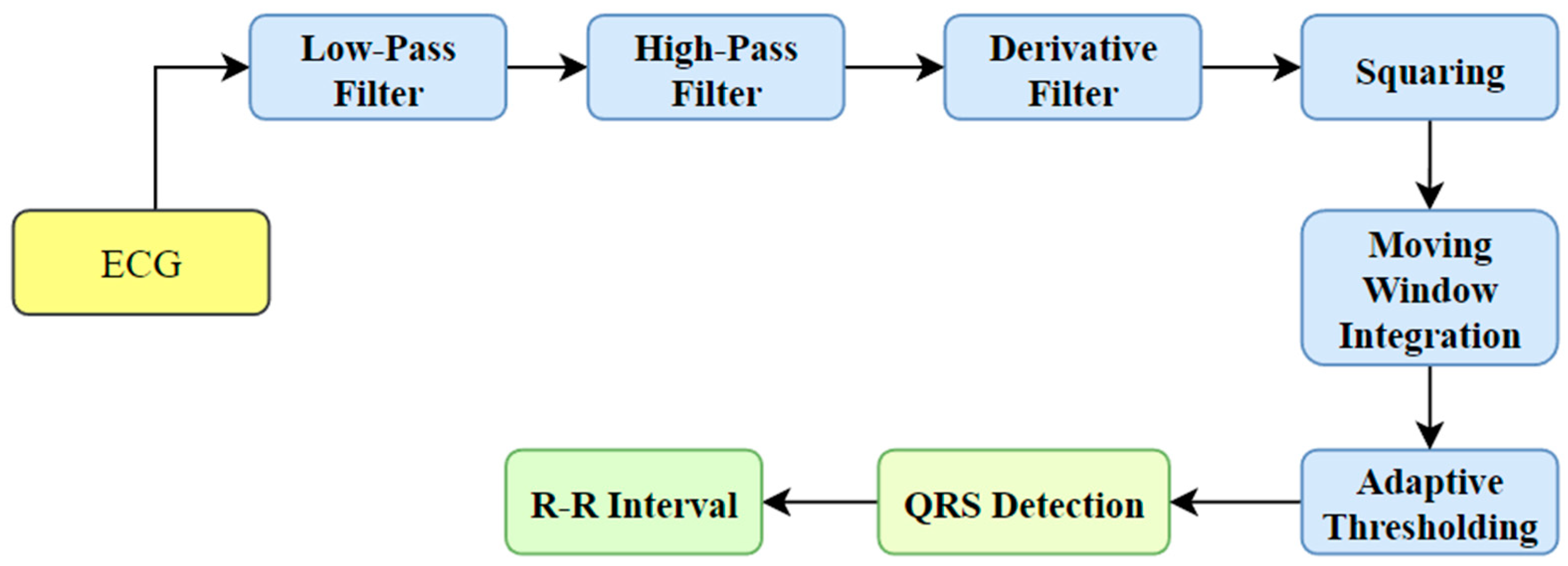
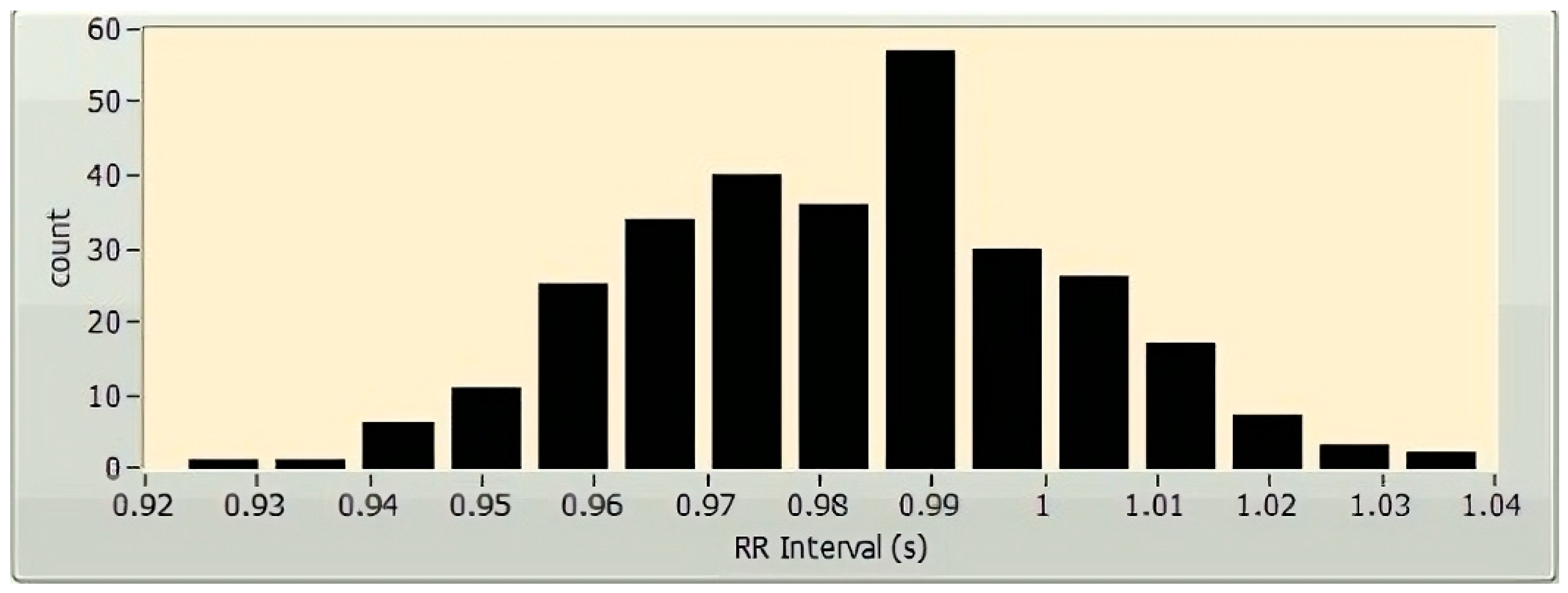
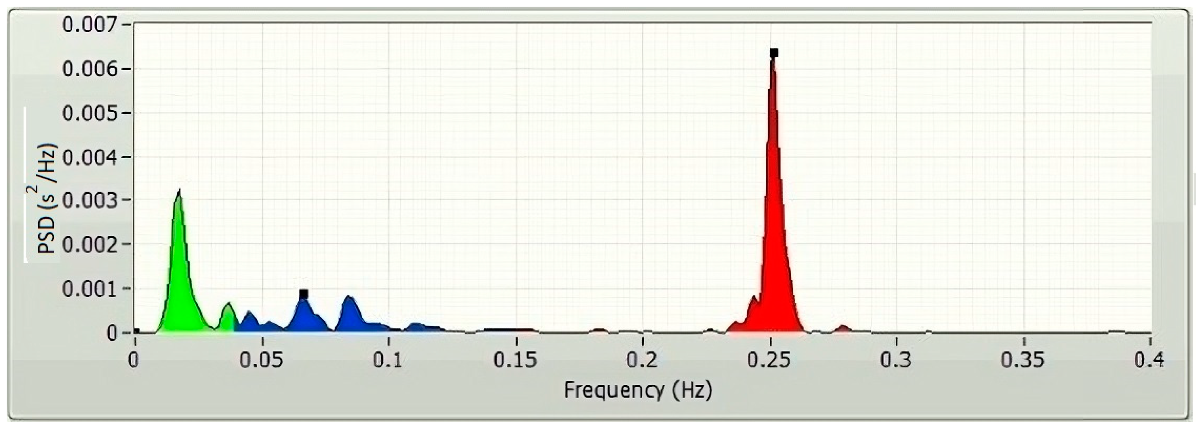
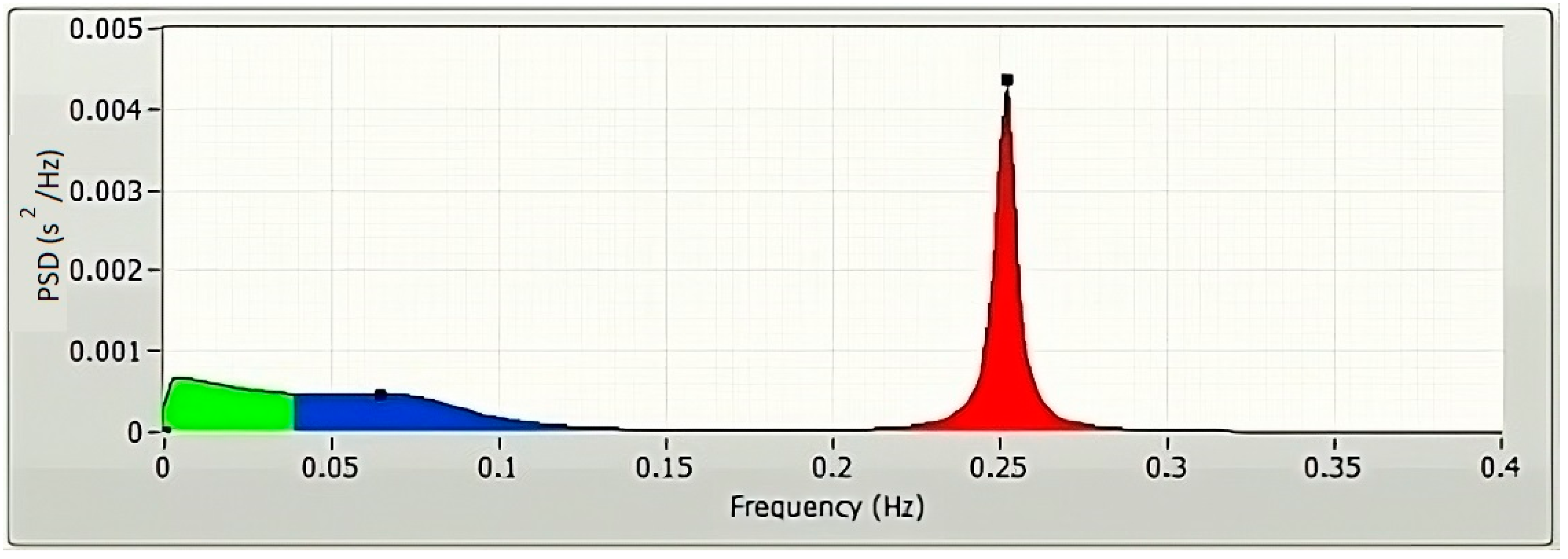
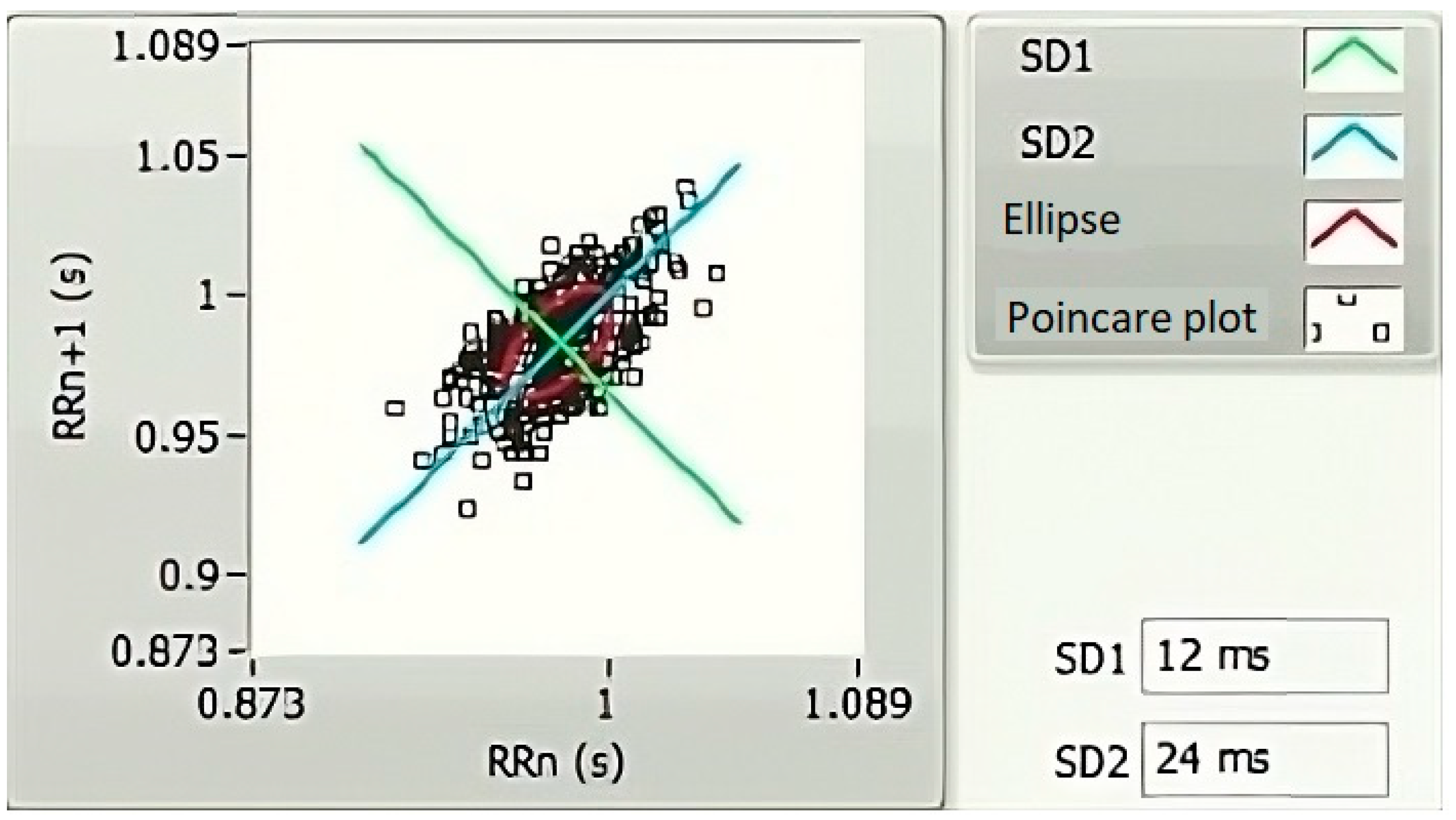
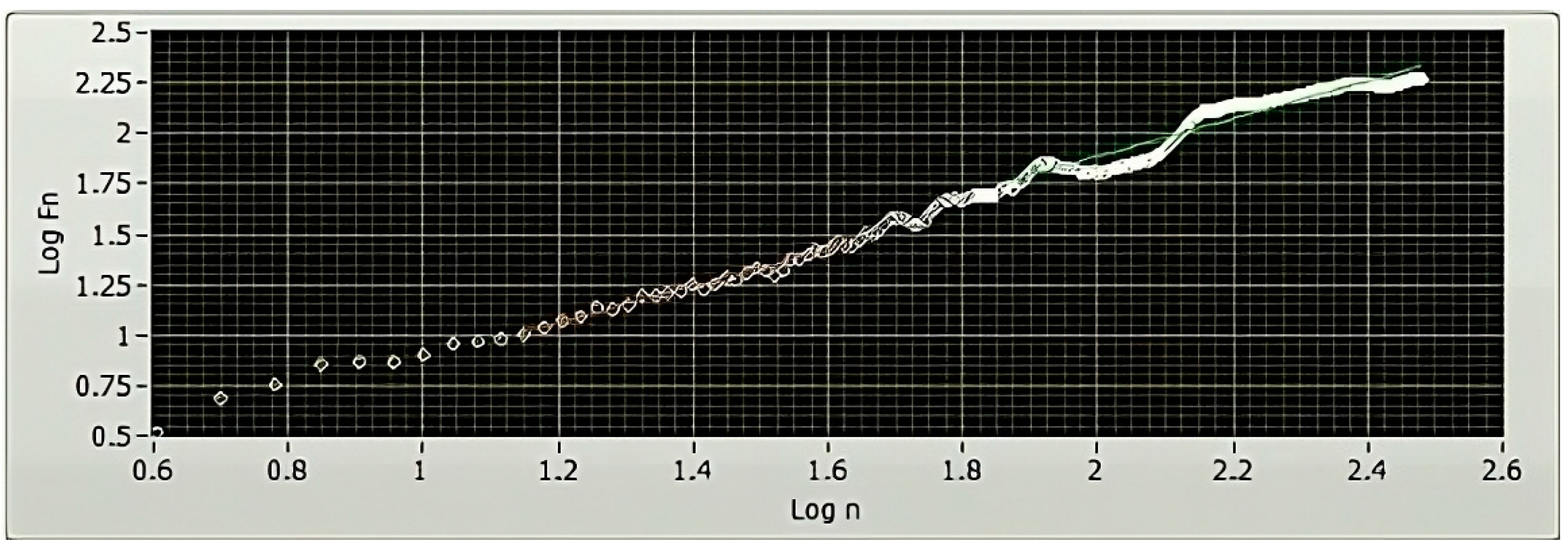
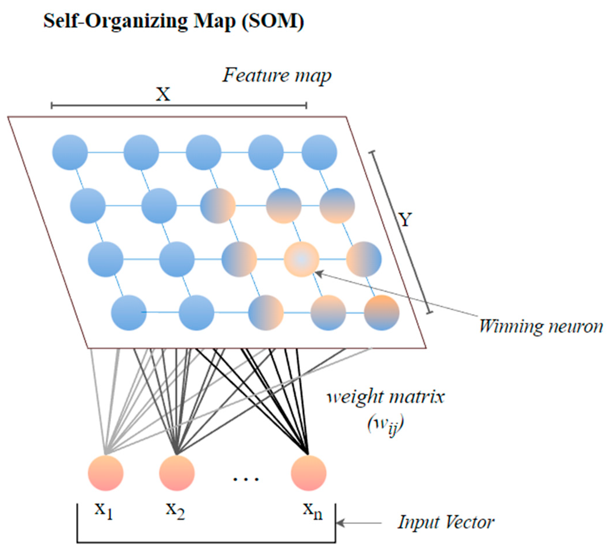
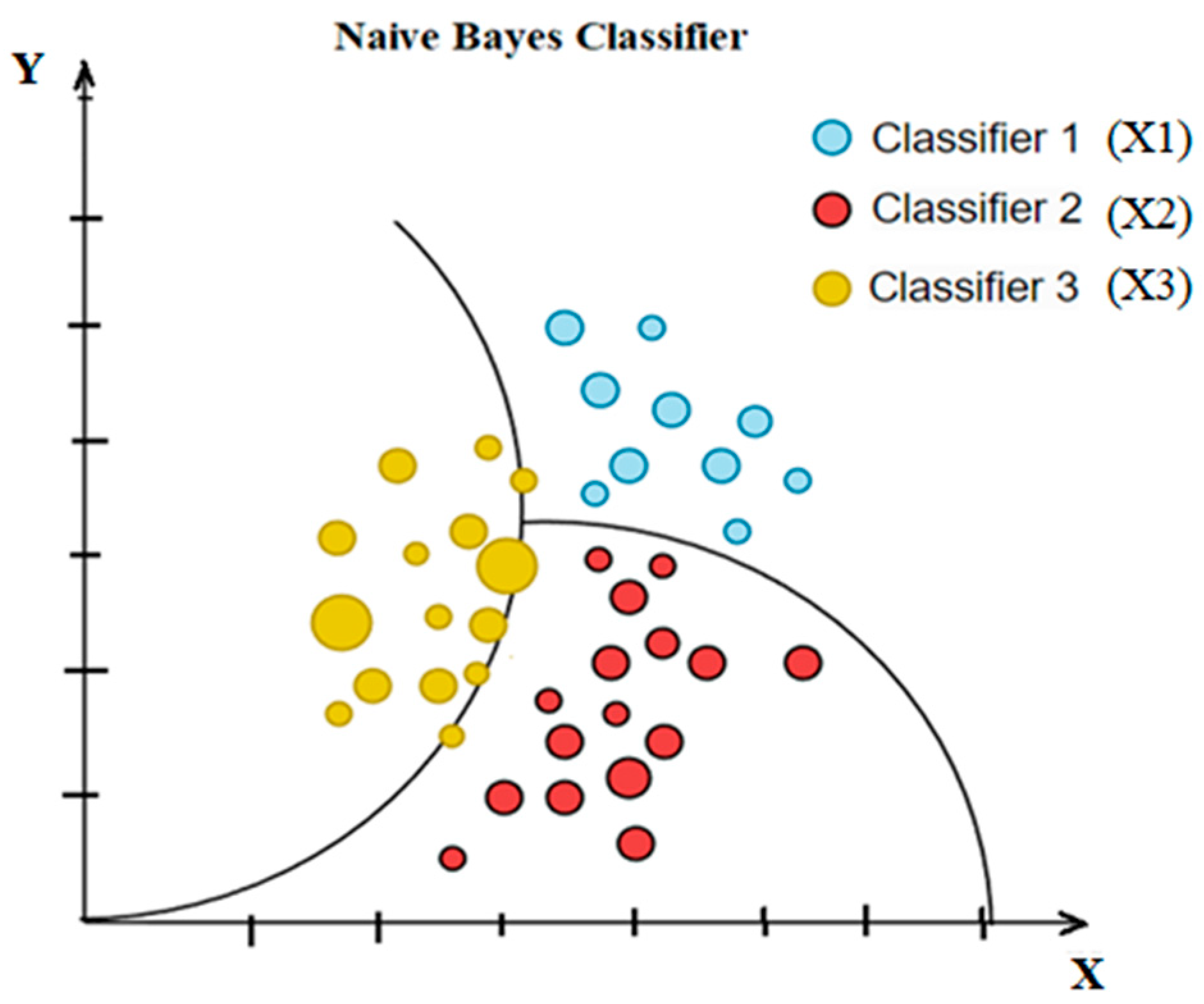
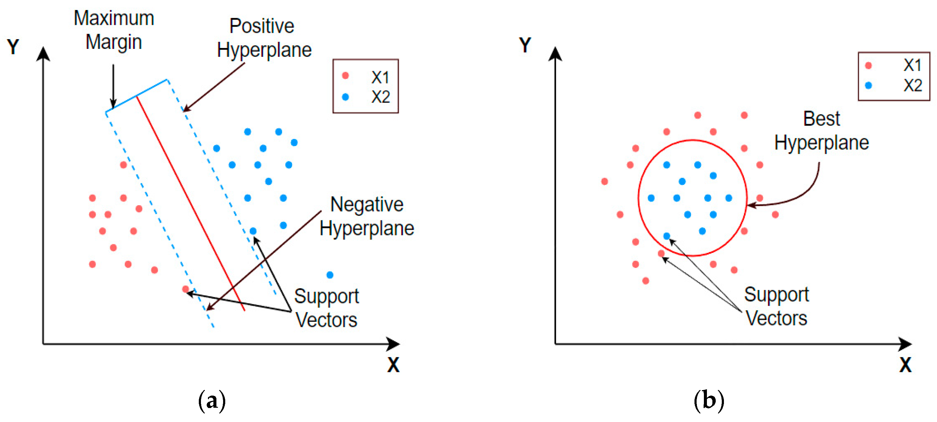
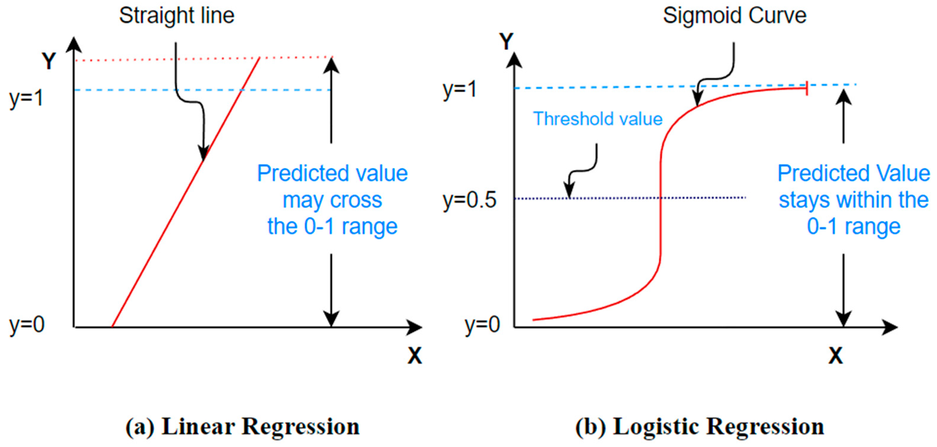

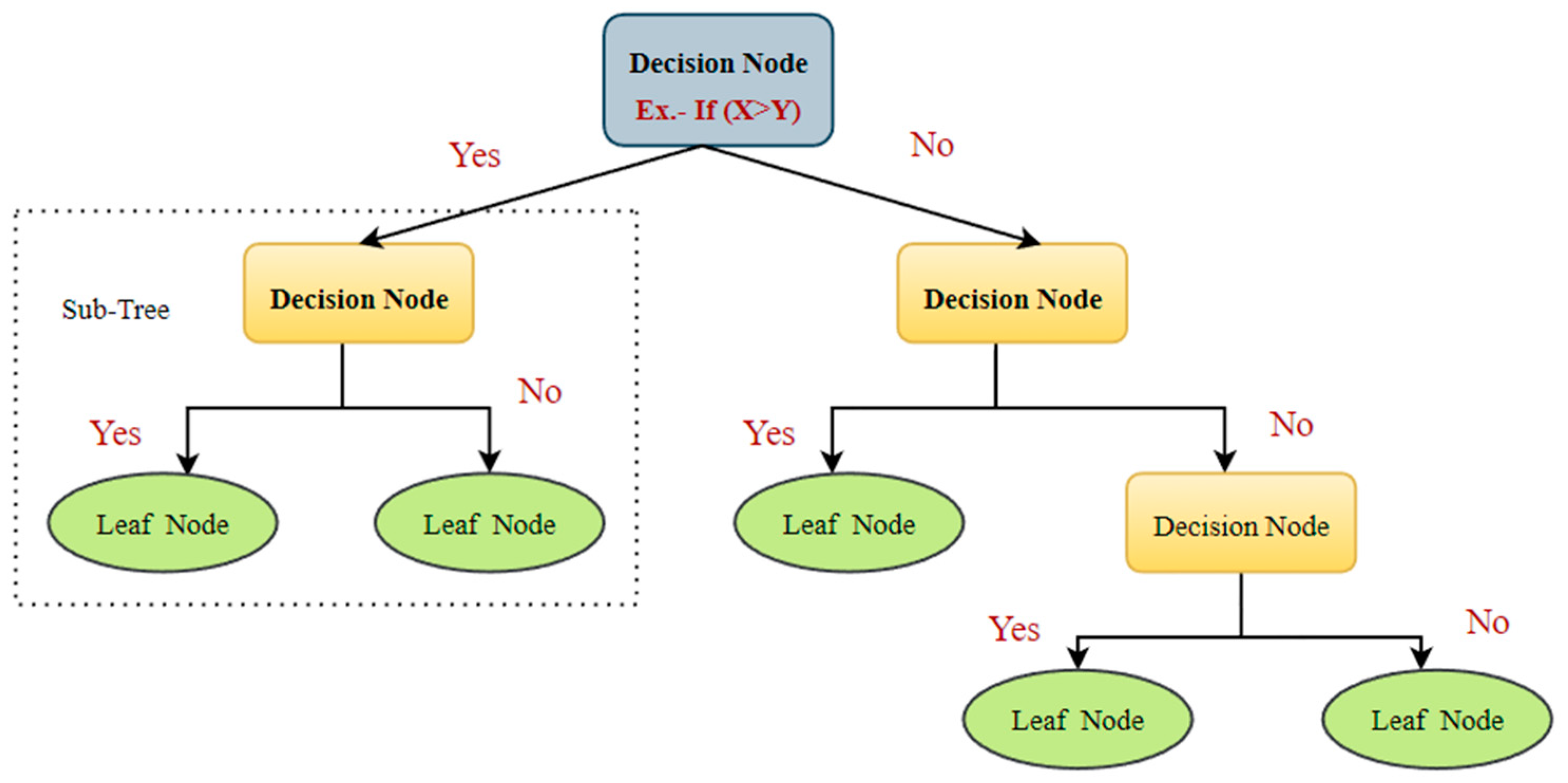
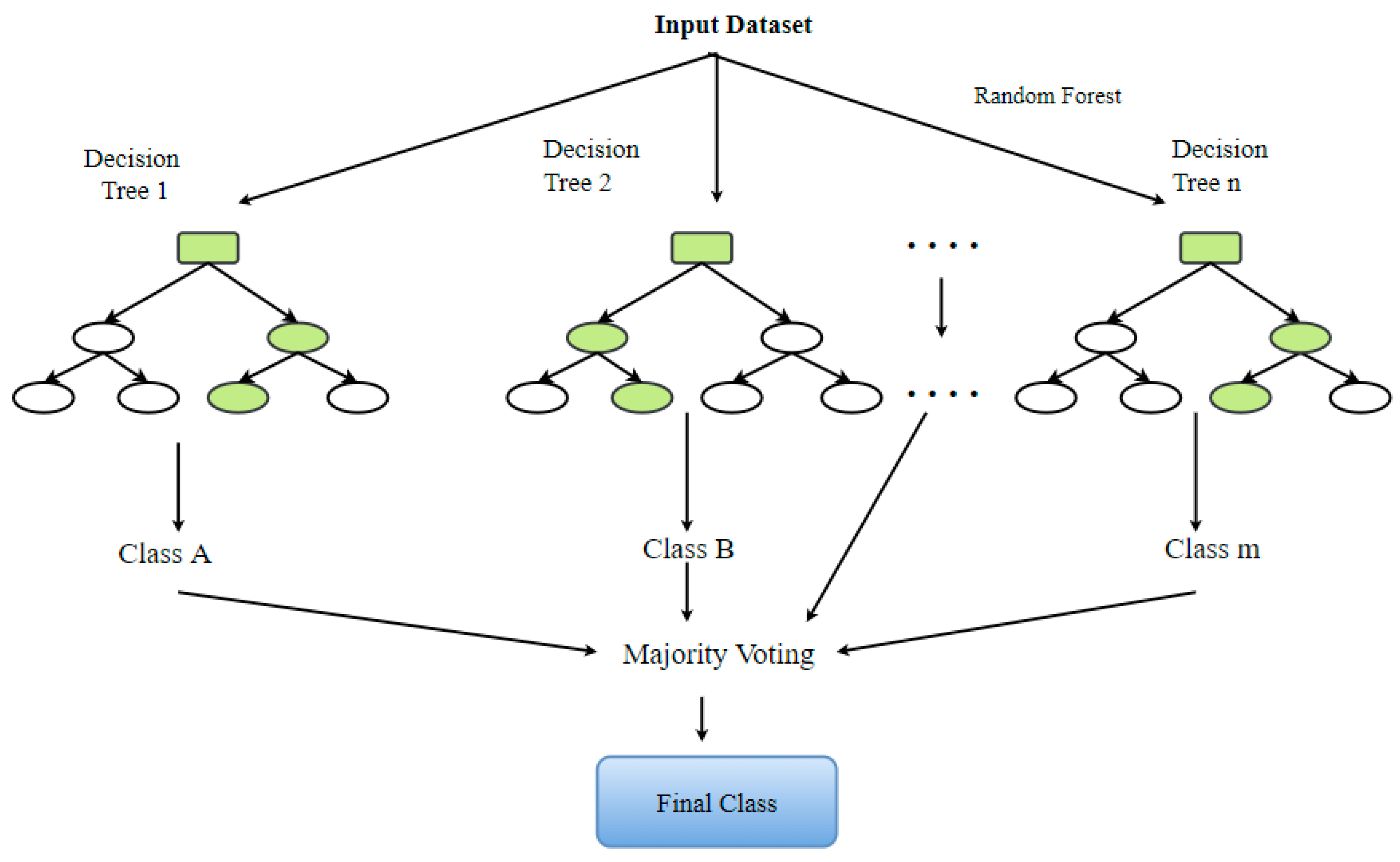
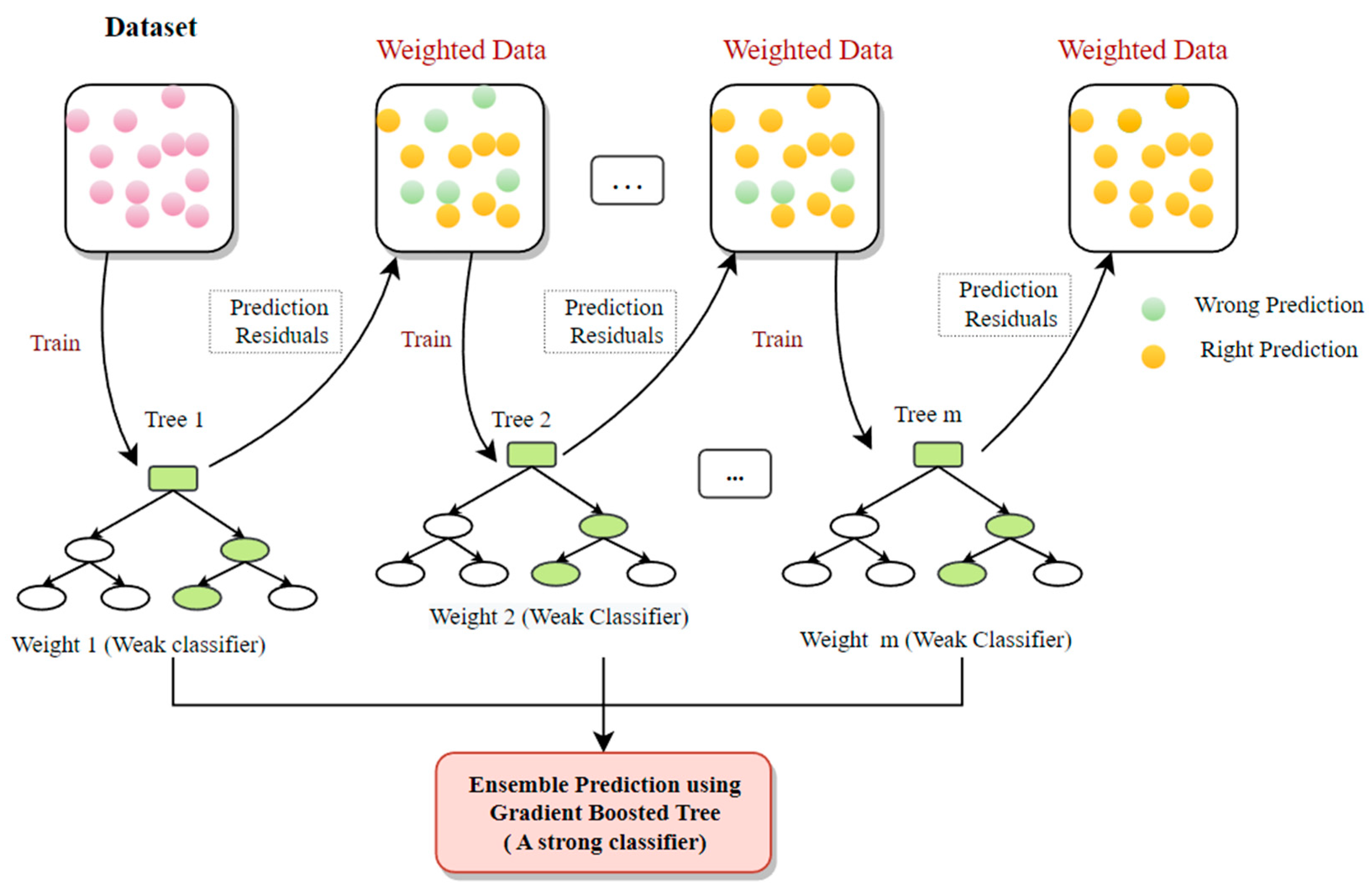
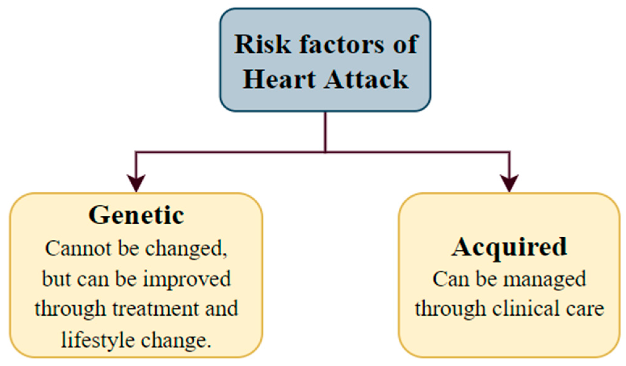
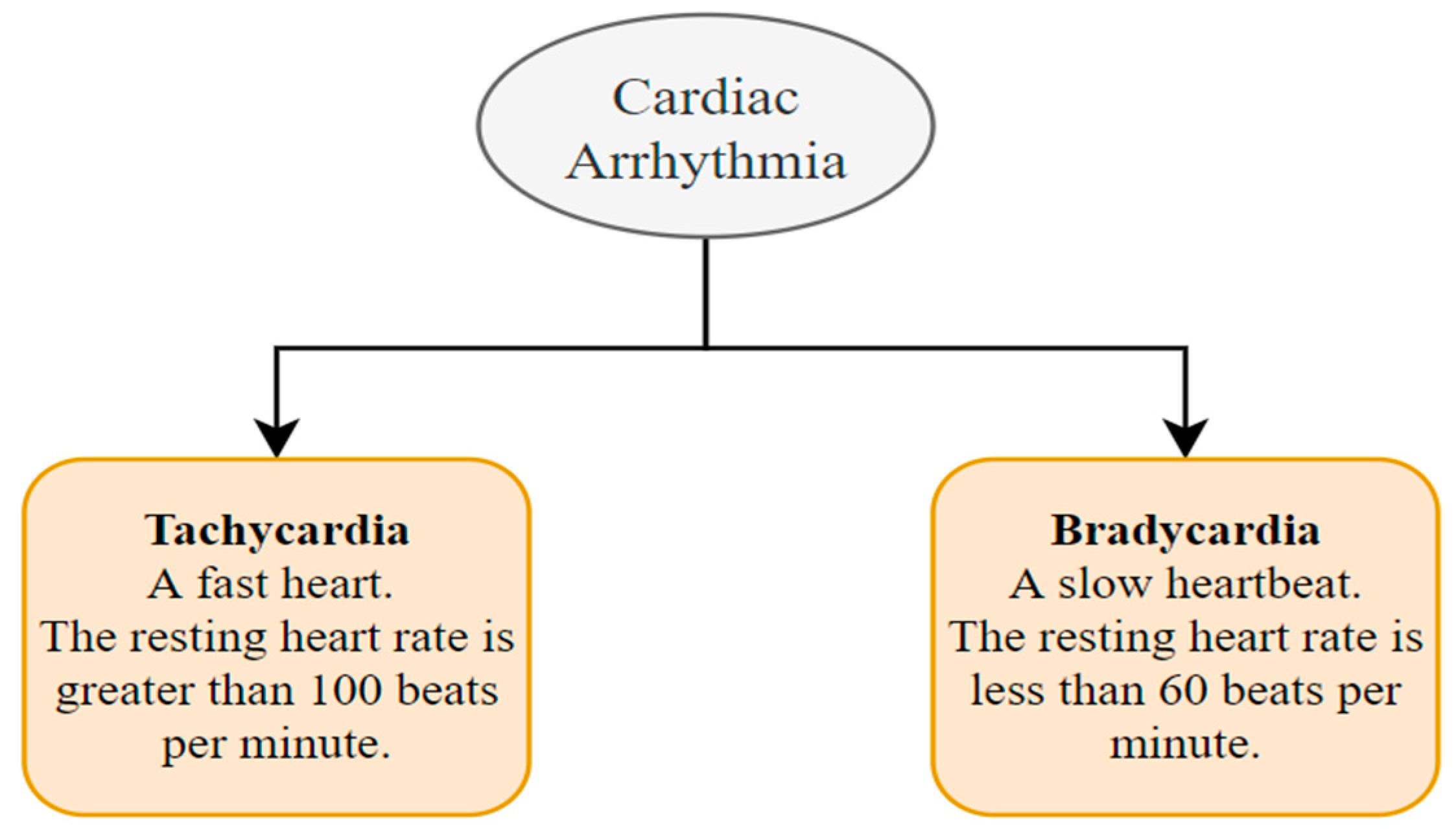
Disclaimer/Publisher’s Note: The statements, opinions and data contained in all publications are solely those of the individual author(s) and contributor(s) and not of MDPI and/or the editor(s). MDPI and/or the editor(s) disclaim responsibility for any injury to people or property resulting from any ideas, methods, instructions or products referred to in the content. |
© 2023 by the authors. Licensee MDPI, Basel, Switzerland. This article is an open access article distributed under the terms and conditions of the Creative Commons Attribution (CC BY) license (https://creativecommons.org/licenses/by/4.0/).