Time-Dependent Unavailability Exploration of Interconnected Urban Power Grid and Communication Network

Abstract

This paper presents a time-dependent reliability analysis created for a critical energy infrastructure use case, which consists of an interconnected urban power grid and a communication network. By utilizing expert knowledge from the energy and communication sectors and integrating the renewal theory of multi-component systems, a representative reliability model of this interconnected energy infrastructure, based on real network located in the Czech Republic, is established. This model assumes reparable and non-reparable components and captures the topology of the interconnected infrastructure and reliability characteristics of both the power grid and the communication network. Moreover, a time-dependent reliability assessment of the interconnected system is provided. One of the significant outputs of this research is the identification of the critical components of the interconnected network and their interdependencies by the directed acyclic graph. Numerical results indicate that the original design has an unacceptable large unavailability. Thus, to improve the reliability of the interconnected system, a slightly modified design, in which only a limited number of components in the system are modified to keep the additional costs of the improved design limited, is proposed. Consequently, numerical results indicate reducing the unavailability of the improved interconnected system in comparison with the initial reliability design. The proposed unavailability exploration strategy is general and can bring a valuable reliability improvement in the power and communication sectors.

1. Introduction

In the ongoing transformation of the energy and communication infrastructure, a marked transition from centralized to decentralized systems can be observed. Concurrently, there is a substantial deployment of smart devices designed for network management, control, and monitoring, further enhancing the interconnection between the energy and communication networks. This enhanced integration is crucial, especially in the context of distribution networks. These networks are essential in ensuring a steady supply of electricity to households, businesses, and industries. It is essential to mention that any disruption in this supply can result in significant financial implications. Not only do Distribution System Operators (DSO) lose profits from such interruptions, but they also face potential penalties imposed by regulators. The efficiency and reliability of distribution networks is therefore of great importance to both consumers and DSOs.

The reliability and consistency of electricity distribution are key characteristics, and their effectiveness is measured using specific metrics, namely the System Average Interruption Frequency Index (SAIFI) and System Average Interruption Duration Index (SAIDI). These indices provide a quantifiable measure of the electricity’s delivery quality to the end users. As the energy sector transitions to decentralized systems and incorporates intelligent network management devices, it is evident that communication devices play a substantial role in influencing these metrics. Specifically, devices such as Remote Terminal Unit (RTU) and Advanced Metering Monitor (AMM) are introduced. These components not only serve as essential interfaces between the distribution network and the control center, but also ensure real-time monitoring and control over the entire grid, encompassing power elements like transformers, lines, and circuit breakers.

To enhance the reliability of the distribution system, one effective strategy is optimizing its maintenance with regard to repair costs, revisions, and the frequency of these tasks. This optimization task, however, becomes considerably more intricate when two interconnected infrastructures, namely the power and communication networks, are taken into account. This paper introduces a novel methodology to calculate the unavailability of the entire system which is crucial for computing SAIFI and SAIDI parameters. Furthermore, we delve into the possibilities of optimizing maintenance on a test network of these interconnected infrastructures, laying emphasis on potential dependencies and interactions during their operation. On the basis of prior research, a mathematical model employing the Weibull distribution is adopted to evaluate system contingencies within this combined infrastructure.

In this research, a key objective is to standardize the terminology associated with reliability parameters relevant to both power grid and communication network systems. It has been observed in various publications that these terms are often misunderstood or inaccurately labeled. When multiple interconnected systems are taken into account instead of a singular system, understanding their interrelationships and dependencies becomes essential. To address this, the paper aims to clarify these relationships using Acyclic Graph (AG), a graphical representation method that has been successfully utilized by the authors in past research, as evidenced by [1].

The rest of the paper is organized as follows. It begins with a discussion of the state of the art in Section 2, where an overview of relevant literature and the results in the field are presented. In Section 3.1, the intricacies of the interconnected infrastructures’ test network are explained. This section provides a detailed description of the devices in these infrastructures and painstakingly delineates their mutual dependencies. As it progresses to Section 3.2, the article is focused on the definition of the system’s optimal function. Here, the maintenance optimization challenges for such interconnected infrastructures take the limelight, and discussion with an interpretation through AG is supplemented. In Section 3.3, the methodology and theory behind the analysis of incident-related Key Performance Indicators (KPI) are summarized. This is performed with the aim to achieve a unified understanding of parameters in congruence with this paper overarching research goals. Section 3.4 focuses on the methods used to ascertain the unavailability of the interconnected infrastructure. Pivotal results are presented in Section 4. Section 5 concludes the paper with a discussion of the model’s limitations and maps the future research, which includes maintenance optimization.

2. State of the Art

The extensive body of literature on the topic underscores the key role of reliability and risk modeling in interconnected infrastructures. This review commences with a thorough assessment of both foundational texts and the most relevant recent studies on the subject.

In [2], the authors undertake an exhaustive survey of more than 150 papers pertaining to Fault Tree Analysis (FTA), thereby rendering an in-depth insight into the state-of-the-art methodologies of FTA. This exploration not only covers the traditional aspects of the Fault Tree (FT), but also discusses its several extensions, including Dynamic Fault Tree (DFT), Repairable Fault Tree (RFT), and Extended Fault Tree (EFT). Reference [3] discusses the mathematical framework behind the optimal allocation and planning of maintenance personnel, casting maintenance optimization as a multi-faceted optimization problem. In another significant contribution [4], a broad spectrum of reliability and risk modeling techniques is introduced. These range from the Conventional Fault Tree (CFT), Event Tree (ET), and Binary Decision Diagram (BDD) to more nuanced methods like Petri Nets (PN), Markov Modeling (MM), and Attack Tree (AT), designed to identify and mitigate the latent risks which are characteristic for Cyber-Physical Systems (CPS).

In line with DFT, a chapter in [5] analyzes the methodology, reviewing popular techniques including Markov chains and Bayesian networks. Systematic review [6] covers Reliability, Availability, Maintainability, and Safety/Security (RAMS) analysis of Critical Infrastructure (CI) papers. Altogether, 1500 papers which cover the RAMS topic published between 2011 and 2020 are analyzed. The target applications include grid stations, cyber-physical systems, cloud computing, software-defined networks, industrial control systems, and Supervisory Control And Data Acquisition (SCADA) systems.

In [7], AT are categorized into two distinct dimensions: (i) proper trees versus directed AG, and (ii) static gates versus dynamic gates. On another front, in [8], a comprehensive overview of reliability modeling in CPS is delivered. This includes highlighting the intricacies associated with reliability and fault modeling across the three core components of CPS: hardware, software, and humans. Furthermore, the authors analyze challenges arising from the integration of these components to offer a holistic approach to CPS reliability modeling. Innovative paper [9] presents a methodology that focuses on deriving repairable multi-state FT from time series fault data. This method is adept at analyzing non-exponential distributions of both reliability and maintainability, and it proves instrumental in predicting the system’s future reliability along with detailing the FT structure. Lastly, in [10], attention is centered on the generation of DFT for systems that incorporate redundancies. These redundancies, commonplace in safety-critical systems, serve the primary purpose of enhancing system reliability. The authors’ objective in this paper is twofold: first, to introduce a redundancy profile, and second, to pave the way for the automatic generation of DFT based on system models.

In recent years, a focus has been placed on software tools tailored for the reliability analysis of systems. The 2017 report on open-source FTA tools, as mentioned in [11], highlighted several tools. Their findings, updated to reflect the current status, list the following tools:

• OpenFTA (Open-source): OpenFTA, an FTA tool, aids in comprehending and applying FTA, a method in safety engineering for qualitative and quantitative evaluation of CI system reliability and safety. However, having not been updated for over a decade, its relevance in contemporary applications might be questionable.
• OpenAltaRica (Restricted free access): OpenAltaRica focuses on risk analysis of intricate systems using the AltaRica language, a high-tier language crafted for the RAMS analysis of systems. Catering to vast models, it encompasses both qualitative and quantitative examination instruments.
• Fault Tree Analyser (Demo version available): A segment of ALD’s suite tailored for reliability engineering and risk evaluation, this tool offers a visual interface for constructing and scrutinizing FT. It is engineered to deduce the likelihood of a principal event from the probabilities of foundational events.
• Isograph FaultTree+ (7-day trial): Crafted by Isograph, FaultTree+ is a leading application for creating FT and executing qualitative and quantitative FTA. Its user-friendly interface is equipped to manage a range of logic gates and incidents. Industries such as defense, aerospace, nuclear, and rail have integrated Isograph’s software suite into their operations.
• Item Toolkit (30-day trial): This suite offers tools essential for reliability predictions—Failure Modes and Effects Analysis (FMEA), FTA, and other reliability engineering undertakings. Designed for analyzing both rudimentary and advanced systems, it aids engineers across domains, from electronics to mechanics, to gauge their designs’ reliability.
• DFTCalc (Open-source): Essentially a “DFT Calculator”, DFTCalc specializes in DFT analysis. Differing from conventional FT that employs just AND and OR gates, DFT encapsulates event sequences and intricate interdependencies. Scripted in C++, DFTCalc yields metrics for reliability and availability for such trees.

Despite a wealth of research, significant discrepancies in the interpretation of KPI persist across several publications [12,13,14,15,16,17,18,19,20,21,22,23,24,25]. With an intent to address and rectify these inconsistencies, in paper [26], the authors propose a time-dependent reliability analysis tailored for a real critical energy infrastructure use case, which consists of interconnected urban electrical and communication network reliability assessment of highly reliable elements, which leverages exact reliability quantification of highly reliable systems. The software presented in this paper can quantify the reliability of very reliable systems up to ${10}^{-45}$, which was demonstrated on a Highly Reliable Markovian System (HRMS) benchmark and also successfully compared with MOCA-RP software [26]. Differentiating from earlier studies, the current investigation of this paper’s authors emphasizes a robust reliability quantification, which is applied to the real interconnected energy infrastructure. The interconnected infrastructure is based on the real system located in the Czech Republic and covers two distinct infrastructures: the power grid and the communication network. For illustrative purposes, the paper introduces a novel version of an interconnected infrastructure test network proposed in [27]. Further, in the realm of time-dependent reliability analysis using AG, pertinent algorithms for discrete maintenance optimization of intricate multi-component systems have been presented in [26]. Given the current discourse in the state of the art, there is an unequivocal demand for specialized software tools that can handle the time-dependent reliability of highly reliable interconnected systems. Pursuing this need, the main aim of this paper is to incorporate the computations related to unavailability into a pre-existing simulator, which has been elaborately discussed in [28].

3. Methodology

This section is devoted to the introduction of the model of interconnected infrastructures, the methodology and theory used in determining KPIs, and the issue of AGs.

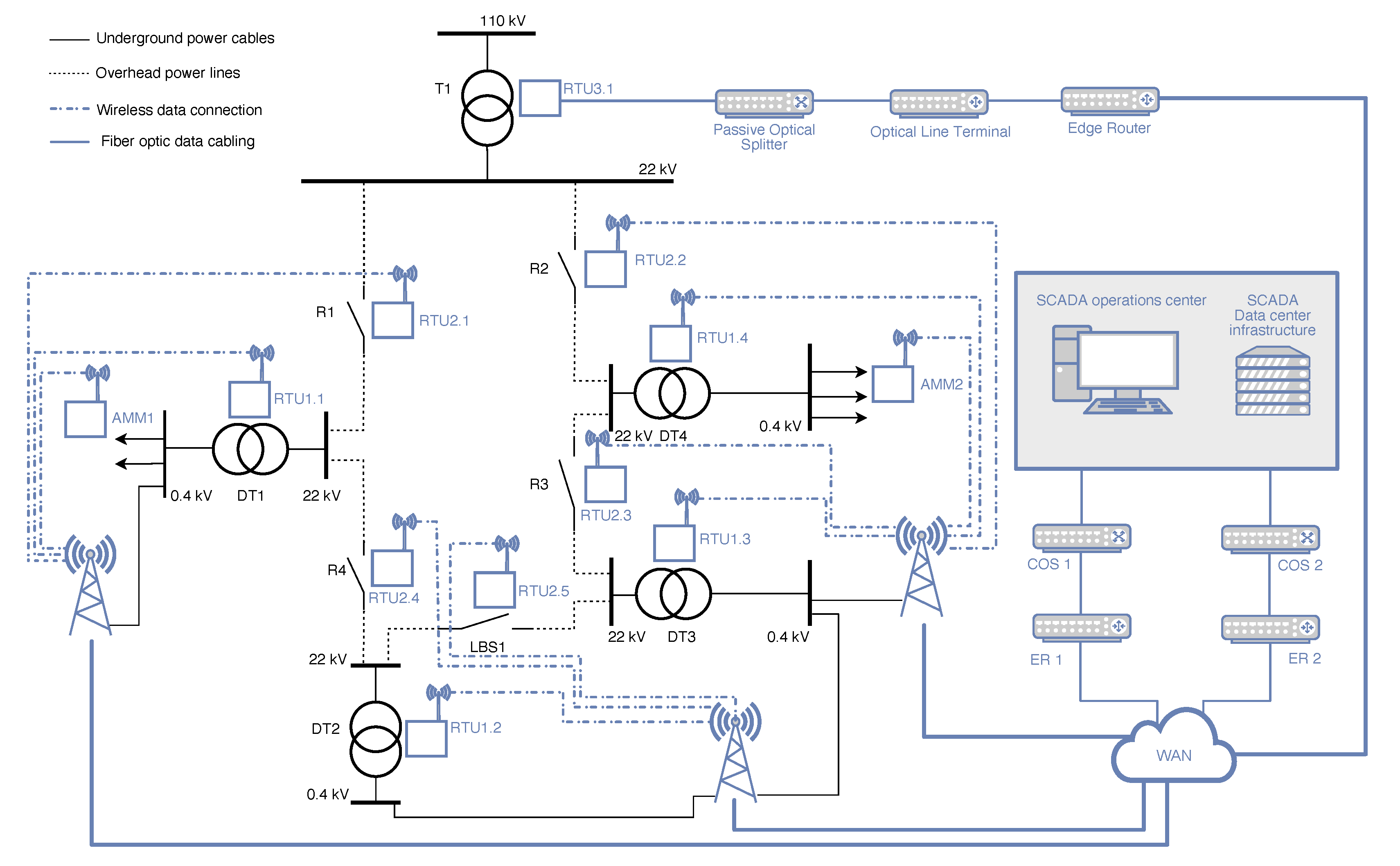
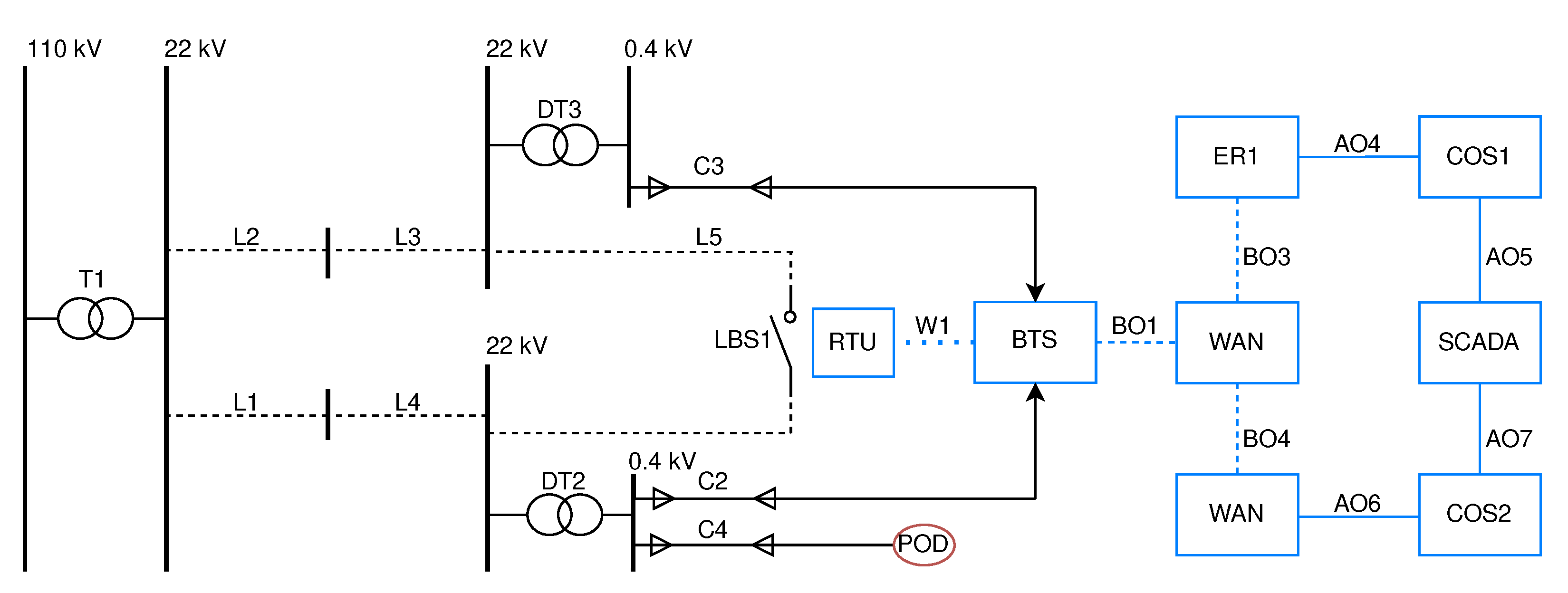
3.1. Description of Representative Infrastructure

The topology of the chosen test network, which encompasses interconnected infrastructures, is illustrated in Figure 1. The network is made up of two autonomously functioning infrastructures: the power distribution network and the communication network. Comprehensive details of each network are elaborated upon in the following subsections. It is imperative to note that there are two unique dependencies between these two infrastructures.

• The reliance of the communication infrastructure on the consistent performance of the distribution network. This is due to the wireless transmitters that source their power from the Low Voltage (LV) level of the distribution system. Specifically, they derive power from LV busbars of the Distribution Transformer (DT) labeled DT1, DT2, and DT3.
• The second dependency emerges from the integration of specific RTU and AMM devices within the distribution network. When these devices malfunction, they can disrupt the distribution system’s operations in two potential ways: (i) directly (by hindering the ability to control switching devices), and (ii) indirectly (through failures of metering devices). It is crucial to note that the influence of AMM devices on the distribution network’s operation is not taken into account for the purposes of this paper because they are exclusively utilized for metering objectives (non-direct impact).

An RTU is a device within industrial control systems that facilitates the remote monitoring and control of various processes and equipment. Its architecture typically encompasses Input/Output (I/O) modules, a central processor, onboard memory, and communication interfaces tailored for seamless connectivity to an array of devices, including but not limited to sensors, reclosers, and load break switches (LBS). To enhance their resilience, RTU often incorporates features such as backup power supplies and redundant communication channels. Nevertheless, they are not immune to faults, and have thus been neglected for the purposes of this paper. These faults, which can significantly disturb the operation of the distribution system, may be based on diverse sources including adverse environmental conditions, inherent hardware and software defects, or lapses in communication. A comprehensive understanding of these factors, coupled with insights into their potential impact on the probability of RTU failures, is imperative. Such knowledge not only bolsters system reliability, but also aids in minimizing the risk of power disruptions and streamlining maintenance strategies. In the context of the aforementioned dependency, the test network accounts for the following four distinct RTU types:

• RTU installed in Medium Voltage (MV) switchboards at Distribution Transformer Stations (DTS), referenced as RTU1.1–4 in Figure 1.
• RTU serving as the control mechanism for reclosers on MV lines, denoted as RTU2.1–4.
• RTU positioned within the High Voltage (HV)/MV substations, labeled as RTU3.1.
• RTU functioning as the monitoring and command unit for section load break switches, identified as RTU2.5.

In DTS, the RTU is responsible for monitoring digital states such as switch positions and door contacts. It enables remote control of feeder switches, offers direct measurement of feeders, and can detect faults within the distribution network. Moreover, the RTU assesses power quality and accumulates data from other electronic instruments present in the installation. In the context of reclosers, the RTU showcases status indicators like recloser status and door contact. It allows for both remote and local control, furnishes 3-phase voltage and current measurements, and is equipped with the capability to detect faults on power lines. Beyond these functionalities, the RTU can handle automatic operations inclusive of protective relays, reclosers, and the management of blocking conditions. For HV/MV substations, RTU plays a crucial role in bridging communication with the SCADA system. This communication is typically facilitated via Ethernet LAN or optical links, but there is an option for a cellular modem backup when needed. The RTU is adept at retrieving data from various substation devices, notably protective relays and power quality meters. When it comes to LBS, the RTU ensures remote and local control of the switch, provides 3-phase voltage and current readings, and detects faults on power lines. An advanced feature includes initiating automatic functions, notably disconnecting after identifying a short circuit during a voltage-free pause, as well as the regulation of blocking conditions.

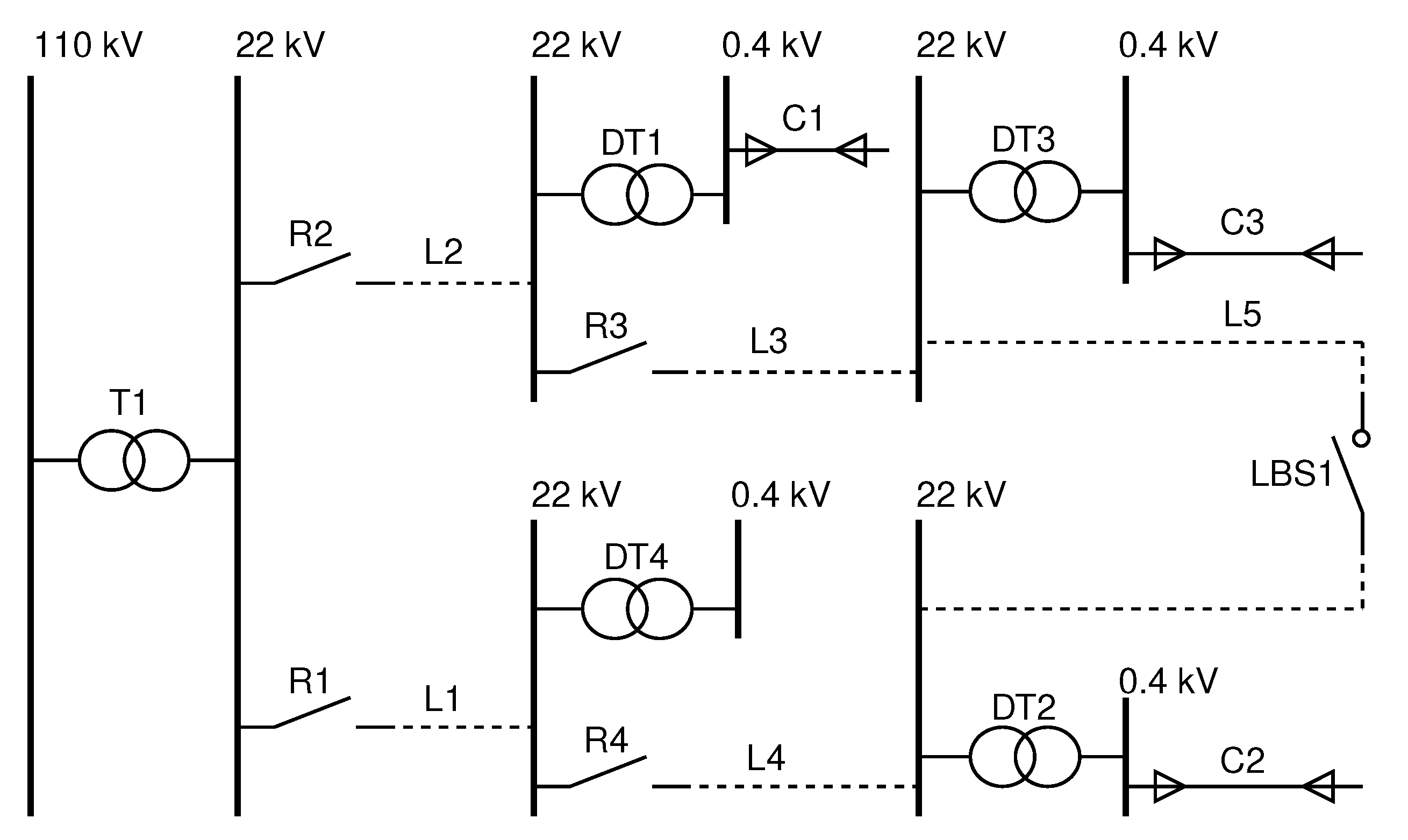
3.1.1. Power Grid Topology

The test network’s power grid part is a representation of a section of the actual distribution network in the Czech Republic, structured with a ring topology, which can be viewed in Figure 2.

Within this grid, there are three distinct voltage levels: the HV segment (110 kV), the MV segment (22 kV), and the LV segment (0.4 kV). Power is supplied to this network from a substation that is equipped with a 110/22 kV transformer. Furthermore, the network consists of five individual sections of overhead lines (L1–L5). Each of these sections is outfitted with a recloser (R1–R4) to interrupt fault currents. The overhead line (L5) is partitioned by a section switch named LBS1. Under normal (fault-free) conditions, this LBS1 is typically in an open state. Hence, the network runs in a radial manner to reduce short-circuit currents. However, if a fault occurs (for instance, in Section L1), section LBS facilitates the DSO to initiate feeding from the other direction. This LBS is operated remotely, and its communication is orchestrated by an RTU, specifically labeled as RTU2.5 in Figure 1. This positions RTU2.5 as a pivotal component for the operation of LBS1. In the event of communication or if RTU2.5 malfunctions, immediate restoration of the supply is impossible due to a fault in the distribution network. Such a scenario results in an extension of the fault duration, subsequently impacting the SAIDI and SAIFI metrics. Moreover, the network houses four DTs (22/0.4 kV) that transform MV to LV, ensuring the demands of the end consumers are met via subterranean LV cables (C1–3). These cables diverge at the LV level busbar and are intended for different consumer groups. This node highlights the dependency of the power network on the communication network, as previously discussed.

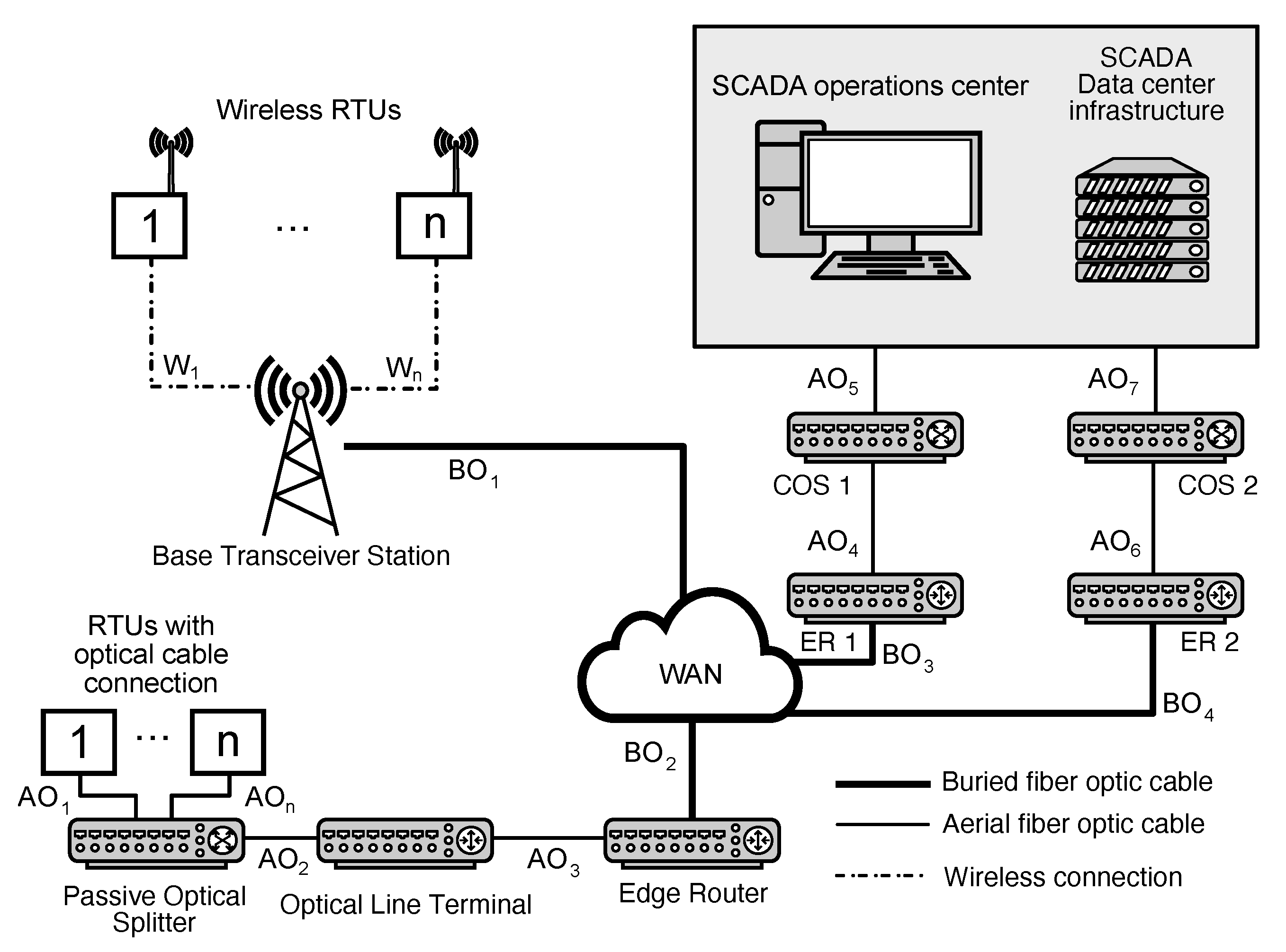
3.1.2. Communication Network Topology

The communication network model, as shown in Figure 3, integrates RTU client devices, segmented into two categories based on their connection techniques. The inaugural category utilizes fiber optics. Devices in this group are interlinked via a Passive Optical Splitter (POS), an Optical Line Terminal (OLT), and ultimately an Edge Router (ER). These routers interface with the Wide Area Network (WAN), which can either be proprietary to the company or a public Internet network. In the case of the latter, communication between the RTU and the server is encrypted and safeguarded by a private Virtual Private Network (VPN) tunnel.

Conversely, the secondary connection method taps into wireless cellular modalities such as Global System for Mobile Communications (GSM), Long-Term Evolution (LTE), or the Fifth-generation broadband cellular network (5G) broadband cellular standard. RTU configured with a mobile network interface is dependent on a modem. All transmissions are encrypted, leveraging VPN tunnels for fortified security, predominantly when transiting public mobile networks. Occasionally, the choice might lean towards a private mobile network. This WAN is directly linked to both a SCADA operational hub and a data repository hosting the requisite server infrastructure for dialogues with the client RTU. While VPN tunnels have the potential to culminate at an ER, high-demand hardware scenarios might necessitate a server exclusively dedicated to VPN liaisons. The role of the SCADA system extends to supervising and orchestrating operations for client networks as well as RTU. Figure 3 represents the diverse connectivity modalities present in the system. The wireless linkages are represented by W ($W_1$ through $W_n$). In contrast, optical conduits are categorized based on their spatial alignment, either above-ground or subterranean. The aerial optical pathways are annotated as AO ($A{O}_1$–$A{O}_n$), and the subterranean optical counterparts bear the BO ($B{O}_1$–$B{O}_n$) notation.

3.2. Description of Network Functionality and Network Contingency Quantification

Unintended power outages are invariably unwelcome due to the associated costs arising from the duration of the disruption. Components of CI are significantly dependent on electrical power. In the event of power disruptions to these CI components, the consequent financial consequences can be significant. Moreover, extended or large-scale outages can bring in not just financial detriments but also social, cyber, and other multifaceted issues. The optimization effort of this paper primarily aims to minimize these associated losses and curtail the threat risk associated with the malfunction of CI’s crucial components, as detailed in [28]. To delve deeper into the risk concerning the power failure of such pivotal components and consequently enhance the overall system’s reliability, the paper clarifies these issues using the test network spotlighted in Section 3.1. To commence, it is imperative to define the precise operational dynamics of the entire system. In this regard, this paper defines a Point of Delivery (POD) that is supplied from the LV bus via the C4 cable, which in turn caters to the CI (this could include key data centers or analogous entities). The overarching correct operation of the system is characterized by the seamless electricity transition from the HV stratum right down to the CI’s load junction at the LV echelon. Under this operational definition, specific components such as DT1, DT4, POS, OLT, and relevant conduits, which do not play a decisive role in the outlined function, can be avoided in the holistic test network representation. The topology of this distributed network is visually represented in Figure 4. Given the premise that reclosers (denoted as R1–R4) do not spontaneously interrupt the power supply during malfunctions, they are omitted from the scheme. Nonetheless, the LBS, pivotal for swift backup power provisioning, remains integral and is thus incorporated within the schematic.

For accurate comprehension of dependencies, it is essential to correctly interpret both individual systems and their interconnections. The comprehensive diagram that illustrates these systems, referenced in Figure 4, can be complex and potentially confusing for some. Consequently, this study uses the oriented AG modelling, as it brings clear and unambiguous representation of these interconnected systems.

AGs are graph structures prevalent in both computer science and mathematics. They consist of nodes and directed edges, ensuring there are no directed cycles. Such a design makes them highly versatile and invaluable for a multitude of applications. Not only can they illustrate complex relationships between elements, but they are also instrumental in scheduling tasks based on dependencies. In the specialized domain of power electrical engineering, AGs play a crucial role in various functions:

• Power Flow Analysis: Here, AGs act as a representation of the power flow in a grid. The nodes within these graphs stand for substations, while the edges denote power transmission lines. By using AGs, engineers and researchers can determine the most efficient power flow routes and detect potential bottlenecks within the grid. For a deeper dive into this application, readers can refer to [29,30].
• Maintenance Optimization: Maintenance within the power grid often requires intricate scheduling to account for dependencies and constraints. AGs assist in this endeavor by helping to prioritize tasks. With the help of these graphs, it becomes easier to determine which tasks need immediate attention and ensure a systematic and efficient completion sequence. More on this can be explored in [26,31,32].
• Power and Data Outage Modeling: AGs also find their application in modeling power and data outages. In such models, nodes signify the various components of the grid, and edges represent the inter-relationships between them. Through these AG-based models, it is possible to swiftly identify the primary causes of an outage. Furthermore, they provide a roadmap for an effective response strategy to restore either power grids, as discussed in [33], or data networks, as highlighted in [34].

AG showcases the dependencies present within the system, allowing for the identification of pivotal elements integral to the full functionality of the system. In principle, an oriented AG, as the represented system, is structured through nodes and edges, but the implications of nodes and edges in the context of a graph significantly differ from general interpretations.

In this case, there is a comprehensive breakdown of the interpretation of these nodes and edges in accordance with [26]:

• First, the graph is inherently acyclic, ensuring that two directly connected nodes share a singular edge.
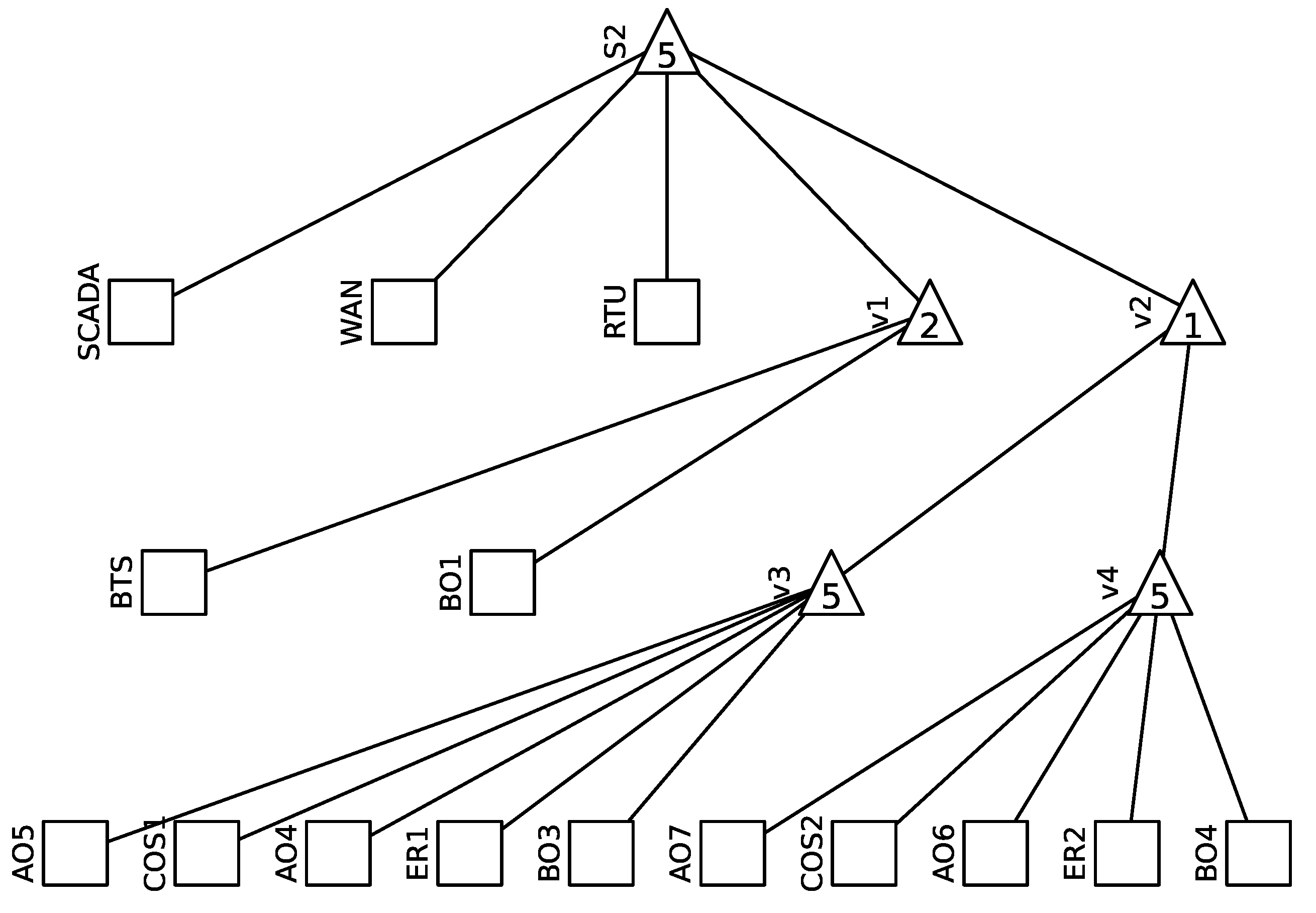
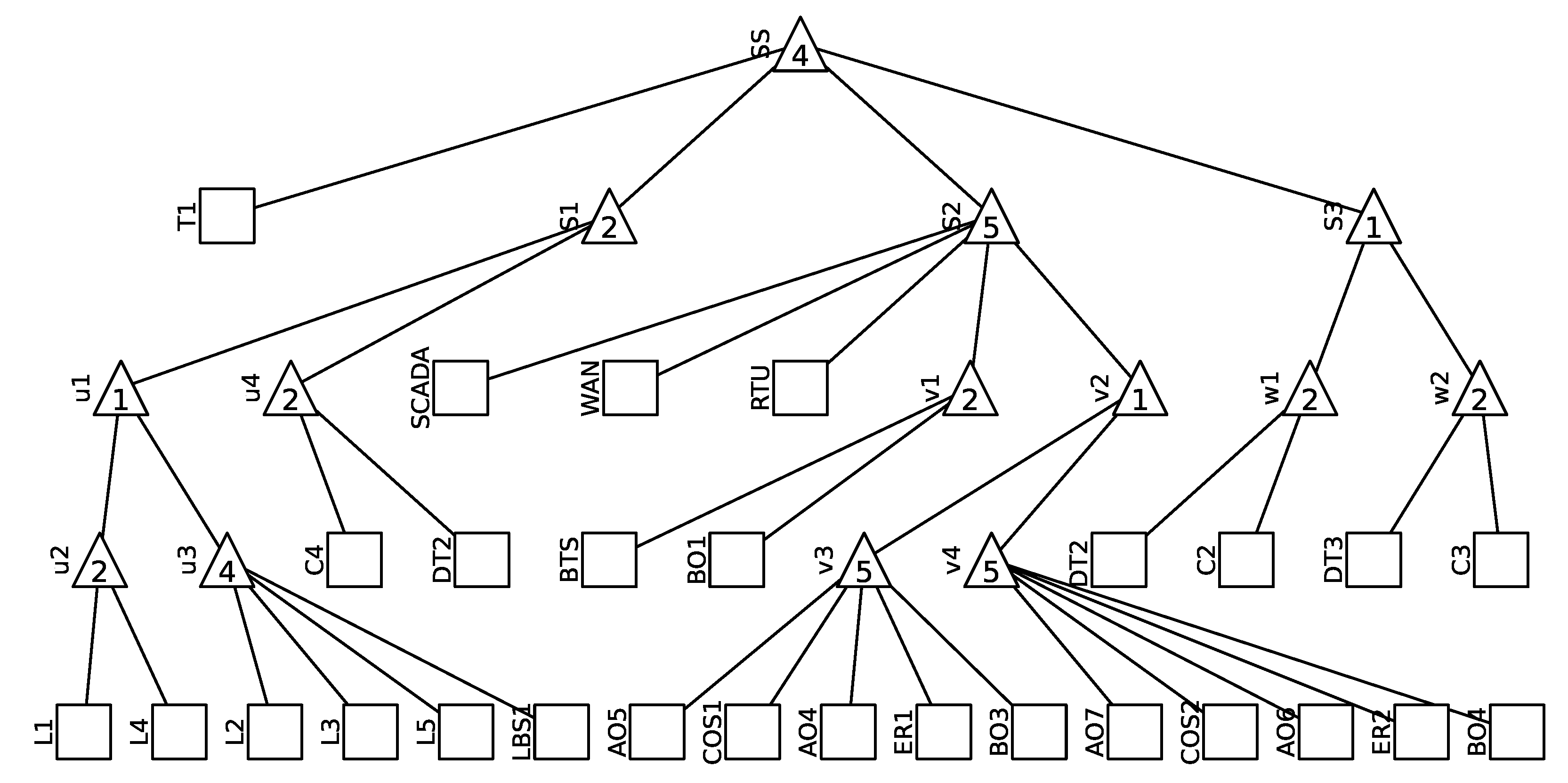
• At the top of the AG is a solitary SS node. This unique node symbolizes the overall system’s functionality, illustrating correct operation against system failure.
• An inherent directionality exists between the nodes of the AG, establishing the relationship of subordination between them, delineated as a slave node in relation to a master node.
• An internal node, also referred to as a non-terminal node, typifies the stochastic behavior inherent within a subsystem. This subsystem is perceived to be in a state of correct functionality only when a minimum of m subordinate nodes (which can either be terminal or non-terminal) concurrently display correct functionality. This stipulation requires the integer m to reside within a specific interval. Specifically:

  −

  The total number of input edges is marked n.

  −

  For a situation where m equals 1, the internal node effectively emulates a logical OR function.

  −

  Conversely, when m matches n, the internal node resonates with a logical AND function.

• The role of terminal nodes is pivotal as they symbolize the operational status of the diverse components integrated within the system. To be precise, these components are subject to events which can either be stochastic in nature or deterministic. For those events characterized by stochasticity, they need to be articulated via distinct probability distributions, specifically catering to the occurrence of faults. Additionally, events tethered to maintenance, either preventive or corrective, necessitate clear and unambiguous specifications.

In the presented case, Node S1 therefore indicates the state where this POD in Figure 4 is supplied. Components that are essential to this state of operation include the C4 cable, the T1 power transformer, and the DT2 distribution transformer. Furthermore, ensuring consistent functionality is a supply pathway, including both lines and LBS. An illustrative representation of the power grid’s structure is shown in Figure 5.

In the test network, as depicted in Figure 4, a similar procedure is administered to the communication segment, which is highlighted in blue. Taking into account the interdependencies between the two infrastructures in the comprehensive test network, the system’s functional correctness is delineated as facilitating LBS operability via the Control Center from the power component of the network. As such, in Figure 4, the pertinent segment of the communication network is emphasized in blue, playing an indispensable role in powering the aforementioned LBS component. Other elements are deemed non-essential for the AG design. The AG tailored for the communication segment of the network, developed in line with the outlined procedure, is illustrated in Figure 6. In this context, solely the interdependencies amidst the constituents of the communication segment are represented within this AG. For the sake of simplicity, both Base Transceiver Station (BTS) and wireless linkage W1 are not accounted for in this depiction, premised on the assumption of their backed-up status, implying they are devoid of failure.

For this demonstration, LV power supply and Distributed Energy Resources (DER) are excluded. Unlike the studies in references [26] that address dependencies within a singular system, this paper faces a challenge when applying the same methodology of constructing an AG to a connected test network treated as two individual systems. Directly combining two AGs is not feasible in this context. Each system has an element from the other, creating a dependency that results in a feedback loop within the graph. By definition, AG cannot have such loops, making the optimization problem unmanageable. To address this, the entire graph is segmented into four subgraphs, each symbolizing a critical subfunction of the complete system.

The system’s reliable operation is fundamentally determined by the consistent and accurate functioning of its four subfunctions. To illuminate the interdependencies in the comprehensive test network, it is discerned that the system achieves its intended performance when each of the following subfunctions is effectively met:

• Function (i): Ensuring that the HV level supplies the MV level, as signified by transformer T1 in the system.
• Function (ii): Guaranteeing a consistent voltage to the MV busbar prior to the Distribution Transformers, as well as ensuring the supply to the critical POD, denoted as u1 in the network.
• Function (iii): Establishing and safeguarding the data communication link between the SCADA operation center and the RTU which oversees the LBS operations in the distribution network. This is represented by subsystem S2 in the system’s configuration.
• Function (iv): Ensuring a stable power supply to the BTS from the MV level. This is facilitated by subsystem S3 through transformers DT2 or DT3 and via cables C2 or C3 in the system architecture.

Taking into account these outlined functionalities, an AG for the comprehensive test network can be conceptualized. It is worth noting that specific elements within this graph might be replicated, such as element DT2. The resultant AG is graphically presented in Figure 7 and forms the foundational basis for the maintenance optimization techniques which is elaborated upon in Section 3.4.

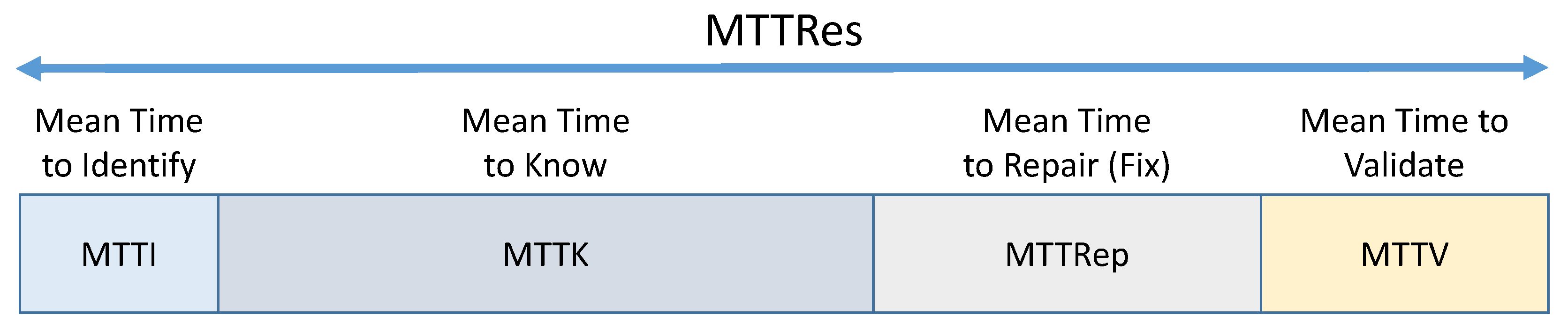
3.3. Theory for Analyzing Incident Key Performance Indicators

In the field of incident management, KPI is instrumental in assessing component performance. As detailed in [12], a large number of KPIs exist. For the scope of the presented analysis, the following indicators are of primary significance:

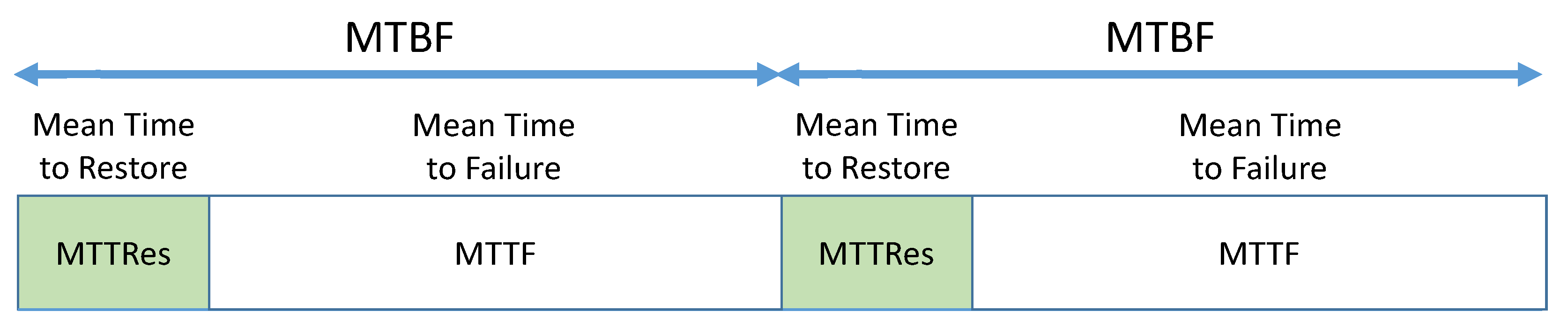
• Mean Time To Failure (MTTF),
• Mean Time Between Failures (MTBF),
• Mean Time To Repair (MTTRep),
• Mean Time To Restore service (MTTRes).

It is imperative to recognize that KPI terminologies and definitions can diverge notably among different suppliers and sectors. The association between these parameters, as detailed across multiple sources, is depicted in Figure 8 and Figure 9. In the first figure is the connection between MTTRes, Mean Time To Identify (MTTI), Mean Time To Known issue (MTTK), MTTRep, and Mean Time To Validate (MTTV), while the subsequent figure emphasizes the relationship between MTBF, MTTRes, and MTTF. In the domain of incident management, MTBF and MTTF stand as paramount reliability metrics. These metrics offer insights into two distinct aspects: the expected time interval between two successive failures (MTBF) and the anticipated duration until a component’s initial failure (MTTF). A salient distinction exists between them.

MTTF is predominantly applied to components that necessitate immediate replacement subsequent to a failure, and it is mathematically represented as

$$\mathrm{MTTF}=\frac{\Sigma T}{\Sigma n_f},$$

(1)

where $\Sigma T$ signifies the total operating time and $\Sigma n_f$ signifies the number of failures.

Shifting the focus to the assessment of system availability, incident management teams generally concentrate on two primary KPIs: MTTRep and MTTRes. The former, MTTRep, elucidates the mean duration required to mend a system following the detection of a failure. It is defined as

$$\mathrm{MTTRep}=\frac{T_{rep}}{\Sigma n_r},$$

(2)

where $T_{rep}$ signifies the cumulative time allocated for repairs and $\Sigma n_r$ signifies the number of repairs. Contrastingly, MTTRes is indicative of the average time consumed to restore a system to its full operational capacity post incident. It is articulated as

$$\mathrm{MTTRes}=\frac{\Sigma T_{res}}{\Sigma n_r},$$

(3)

where $T_{res}$ signifies the cumulative time allocated for restoring system operation. Lastly, MTBF finds its application with components that can be refurbished following a failure. Its definition is

$$\mathrm{MTBF}=\mathrm{MTTF}+\mathrm{MTTRes}.$$

(4)

To accurately evaluate the availability and reliability of interconnected infrastructure, it is essential to concentrate on the most relevant parameters. In this regard, three pivotal parameters are identified for the analysis: MTTF, MTBF, and MTTRes. These metrics offer invaluable insights and present the most lucid information.

Employing this consolidated methodology facilitates a better usage of KPI parameters. These parameters are related to events that impact the interrelated components of the infrastructure, encompassing power, communication, and control systems. This strategy not only deepens the comprehension of the foundational issues and their mutual interplay, but also amplifies the efficacy in troubleshooting and resolving events.

The examined representative interconnected infrastructure is divided into three primary sections: (i) the power grid, (ii) the communication segment, and (iii) the control segment. For the context of this paper, Segments (ii) and (iii) are assessed collectively. The elements of Segment (i) are specified as follows:

• HV/MV transformer (110/22 kV) labeled T1 is determined according to [26] as MTBF 26,310.709 h and MTTRes 4.403 h. The numbers are derived from study [17]. In the paper, “MTBF” corresponds to MTTF, and “MTTR” corresponds to MTTRes.
• MV/LV transformer (22/0.4 kV) labeled as DT2–DT3 is determined by study [17], where the study introduces MTBF 43,800.361 h and MTTRes 0.361 h for MV/LV transformers.
• Load break switch (LBS1) on 22 kV overhead line is determined from study [17], where all power switches are generalized under one category. The study introduces MTBF 224,621.087 h and MTTRes 5.702 h for 22 kV switches.
• Overhead MV line (22 kV) labeled L1–L4 is determined as a MTBF per km and MTTRes. The numbers are collected from various studies in [18,35,36,37,38,39,40] that introduce MTBF between 41,714.286 and 62,571.429 h and MTTRes 11.417 h (as “$\tau$”) for 22 kV overhead lines.
• Underground LV cable (0.4 kV) labeled C2–C4 is determined by MTBF per km and MTTRes from [18,35,36,37,38,39,40], which generalized LV under 11 kV power line cables from various sources in the literature.

Equations (1) and (4) are then utilized to calculate the MTTF and MTBF parameters for cables and overhead lines, with adjustments made for the lengths of the individual sections. The summary table for these components is presented in

Table 1. Characteristic values of power grid components.

Component	MTBF (h)	MTTRes (h)	$\mathit{\beta }$ (-)
Transformer T1 (110/22 kV)	26,310.709	4.403	2
Distribution transformer DT2 (22/0.4 kV)	43,800.361	0.361	2
Distribution transformer DT3 (22/0.4 kV)	43,800.361	0.361	2
Load break switch LBS1 (22 kV)	224,621.087	5.702	2
Overhead line L1 (22 kV)	54,750.000	11.417	2
Overhead line L2 (22 kV)	41,714.286	11.417	2
Overhead line L3 (22 kV)	62,571.429	11.417	2
Overhead line L4 (22 kV)	48,666.666	11.417	2
Overhead line L5 (22 kV)	43,800.000	11.417	2
Underground cable C2 (0.4 kV)	57,737.828	85.000	2
Underground cable C3 (0.4 kV)	38,491.886	85.000	2
Underground cable C4 (0.4 kV)	153,967.543	85.000	2

, which also includes the $\beta$ parameter required for unavailability calculations. The $\beta$ values are adopted from [26] for all devices in the power grid.

This study also follows with the summary of the components of (ii)–(iii) which is shown in

Table 2. Characteristic values of the communication and control components.

Component	MTBF (h)	MTTRes (h)	$\mathit{\beta }$(-)
Edge Router ER1	16,246.780	0.780	2
Edge Router ER2	16,246.780	0.780	2
Core Optical Switch COS1	5,000,014.000	14.000	2
Core Optical Switch COS2	5,000,014.000	14.000	2
Aerial Optic fiber AO4	500,000.000	6.000	2
Aerial Optic fiber AO5	1,093,750.000	6.000	2
Aerial Optic fiber AO6	500,000.000	6.000	2
Aerial Optic fiber AO7	1,093,750.000	6.000	2
Buried Optic fiber BO1	821,875.000	12.000	2
Buried Optic fiber BO3	1,753,333.333	12.000	2
Buried Optic fiber BO4	1,753,333.333	12.000	2
Remote Terminal Unit RTU	100,048.000	48.000	2
SCADA operation and data center	175,200.000	184.600	2
Base Transceiver Station BTS	100,000.000	4.000	2
Wide Area Network WAN	100,000.000	4.000	2

. These components are obtained and defined as follows:

• ER is determined from study [19], which introduces the values MTTF and MTTR for the edge and core router. However, the representative architecture introduced in this paper’s case brings together the ER and the Core Router (CR), so it is more accurate to obtain the numbers for the “core” router. The authors use the same methodology and provide clear values for MTTF and MTTRes (as “MTTR”). Therefore, Equation 4 is used to determine the MTBF.
• Indicators for Optical Line Terminal, Passive Optical Splitter, and Core Optical Switch are all determined from study survey [20]. The study introduces the Failure In Time (FIT) values and MTTRes (as “MTTR”) and the relationship between FIT and “MTBF” (or as defined in the proposed methodology, MTTF in hours):

  $$\mathrm{MTTF}=\frac{{10}^9}{\mathrm{FIT}}.$$

  (5)
  Equations (4) and (5) are used to obtain the required values. The study uses four sources, but only one source contains all necessary information for all three components. Therefore, values marked as “b-Chen1” from [21] are used for the purposes of this paper.
• The optic fiber communication link is divided into a buried link labeled BO1-BO3 and an aerial link labeled AO1-AOn. The indicators are obtained from [22], where the authors published three values for various scenarios: optimistic, nominal, and conservative. Nominal values are used, considered per km for their study.
• Remote terminal units labeled RTU1-RTUn (as well as advanced metering meter, AMM1-2) are determined from studies [23,24], where MTTF (as “MTBF”) and MTTRes (as “MTTR”) are given. Therefore, Equation (4) is used to determine the missing parameter MTBF.
• In this study, SCADA operations and data centers are put together to represent one central system. Parameters are obtained from [25] (defined as “control system”), where the author provides values MTTF and MTTR with the same methodology. Then, Equation (4) is used for MTBF.

For this part of the network, parameter $\beta$ is determined based on the authors’ previous experience with modeling the lifetime of communication elements.

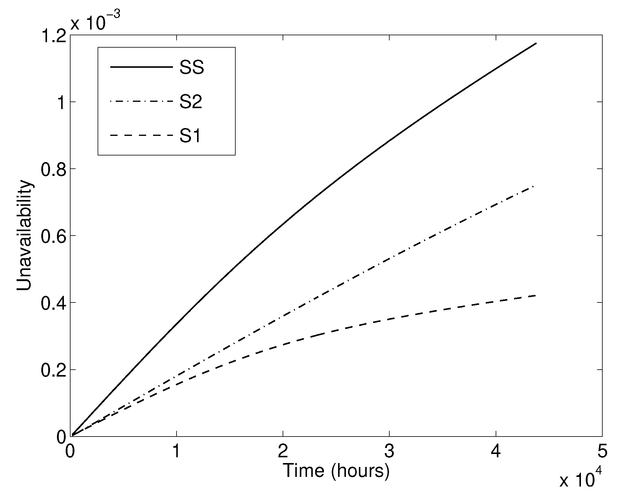
3.4. Theory for Computing Unavailability of the Investigated Infrastructure

This section clarifies the method for calculating the unavailability of the interconnected infrastructure system detailed in previous sections. In Section 3.2, the system was depicted using AGs. Here, internal nodes, represented as triangles in Figure 7 (e.g., u1 or u2), symbolize sub-systems within the network. At any given moment, subsystems and components (which are the internal and terminal nodes, respectively) can either be operational or in a failed state, which may be under restoration. A node is deemed operational if the number of its child nodes matches or surpasses the count encapsulated within the triangle; if not, it is categorized as non-functional. For illustration, Node u1 in Figure 7 is operational if either one or two of its directly subordinate nodes are functional. Understanding the unavailability functions of terminal nodes facilitates the calculation of the unavailability functions for internal nodes. Both of these functions are crucial inputs when determining the unavailability function of the entire network, denoted by the SS node U(t). This function, U(t), offers insight into the time-dependent likelihood that the network might experience failure at time t due to a malfunction or an ongoing repair process.

Model for Unavailability Exploration of a Terminal Node with Corrective Maintenance (CM)

To ascertain the unavailability function of the SS node, U(t), a model and algorithm for quantifying the unavailability of terminal nodes undergoing CM is essential.

In the context of CM, it is crucial to acknowledge two complementary random variables: the lifetime X, characterized by either distribution function F(t) or Probability Density Function (PDF) f(t), and the time needed for repair or recovery Y, described by either distribution function G(t) or PDF g(t). Based on renewal theory and alternating renewal processes, unavailability function U(t) can be expressed as follows [1]:

$$U\left(t\right)=1-A\left(t\right)=F\left(t\right)-{\int }_0^{t}h\left(x\right)[1-F(t-x)]dx,$$

(6)

where U(t) denotes the instantaneous time-dependent unavailability function, A(t) denotes instantaneous availability function, while h(x) represents the renewal density of the pertinent alternating renewal process.

Calculating unavailability using Equation (6) demands familiarity with h(x). This can be intricate since it is numerically represented as an infinite sum of probability densities, each calculated as a convolution.

Nonetheless, this equation can be substituted with its counterpart, termed the recurrent linear integral equation, as elucidated in [1]:

$$U\left(t\right)={\int }_0^{t}f\left(x\right)[1-G(t-x)]dx+{\int }_0^t(f\ast g)\left(x\right)(t-x)dx.$$

(7)

In this context, * signifies convolution. The efficacy of this methodology for determining unavailability in multifaceted and highly reliable systems is validated in [1]. Once all imperative parameters are ascertained, this culminating model can be harnessed to analyze the reliability of distinct components within the network. The Weibull distribution, prominently utilized in reliability engineering, is chosen to model lifetime X. This distribution is discerned by two specific parameters [26]:

• Scale parameter $\theta$, which delineates the typical lifespan of a system or component.
• Shape parameter $\beta$, dictating the distribution’s profile.

When $\beta$ is less than one, the distribution indicates a diminishing failure rate. A $\beta$ of one signifies a consistent failure rate, typically illustrating random failures. Conversely, a $\beta$ value greater than one connotes a surging failure rate, often corresponding to wear-out failures. Specifically, for $\beta$ equal to two, there is a linear rise in failure rates as systems age, commonly seen in electrical components influenced by factors like intensive load or the surrounding environment. The Weibull distribution’s PDF is defined as follows [26]:

$$f(x;\theta ,\beta )=\left\{\begin{array}{cc}\frac{\beta }{\theta }{\left(\frac{x}{\theta }\right)}^{\beta -1}{e}^{-{(x/\theta )}^{\beta }}\hfill & x\ge 0,\hfill \\ 0\hfill & x<0.\hfill \end{array}\right.$$

(8)

Its Cumulative Distribution Function (CDF) is expressed as

$$F(x;\theta ,\beta )=1-e^{-{(x/\theta )}^{\beta }}.$$

(9)

Within electrical engineering, recovery time Y is predominantly characterized by either a rectangular or exponential distribution. Notably, the exponential distribution, predicated upon MTTR specifications derived from authentic data, is favored for network components [26].

4. Results

Using the knowledge summarized in the previous chapters, calculations of the evolution of system unavailability were performed for several scenarios described in this chapter. First, calculation was performed for a separate part of each infrastructure, i.e., the power grid and the communication network separately.

Figure 10 shows the unavailability progression of the power grid (a) and the communication network (b) over a 5-year duration. It can be seen from this figure that the communication network unavailability over a 5-year horizon is almost twice as high as that of the power grid.

Figure 11 shows graphically the aforementioned evolution of the unavailability comparison for systems S1 and S2. Furthermore, the unavailability calculated for the complete interconnected infrastructures represented by the SS system is plotted in this figure. The input for this calculation was the AG shown in Figure 7 in the previous section. From this comparison, it can be seen that in a holistic view of interconnected infrastructures, the impact of both infrastructures on the contingency of the overall system, which increases significantly with interconnection, must be considered.

It has already been mentioned in this paper that the unavailability calculation can also be used for optimization tasks. This fact was demonstrated in another calculation where the S1 system was improved by placing a new transformer, T2 (connected in parallel to transformer T1 in Figure 4).

The calculation of the evolution of the unavailability of such an improved system (S1 improved) is shown in Figure 12, where comparison with the original S1 and S2 systems can be seen (a).

Subsequently, the unavailability calculation of the whole system (denoted as SS improved) is also updated, and comparison with the original SS system is made (b). This comparison shows an improvement in the unavailability of the S1 improved system as the overall unavailability dropped to $2.48·{10}^{-4}$ (originally $4.2·{10}^{-4}$).

All computations were numerically computed using the high-performance programming language MATLAB on computing equipment with the following parameters: Intel (R) Core™ i7-3770 CPU @ 3.4 GHz 3.9 GHz, 8.00 GB RAM.

5. Conclusions

In this paper, a time-dependent reliability assessment of the interconnected system by the renewal theory was provided. Calculations of the 5-year time evolution of unavailability were performed successively, first for the separate systems of the power grid and the communication network and then for the overall interconnected infrastructure.

The presented numerical results show an unfavourably high impact of the power network unavailability (S1) on the overall interconnected infrastructure unavailability, despite the fact that S1 unavailability is lower than the S2 communication network unavailability (see Figure 12).

Numerical results of the time-dependent reliability analysis indicate reduction in the unavailability of the improved interconnected system in comparison with the initial reliability design. It is evident that unavailability reduction is particularly caused by design changes (parallel duplication of Transformer T1).

Figure 12 shows that the unavailability curve of the improved Power grid S1 is significantly lower than those of both S1 original and S2. As a result of this, a significant unavailability reduction in the Interconnected network SS can be observed. Thus, the proposed design brings a valuable reliability improvement, especially to the power grid network of the analyzed interconnected energy infrastructure.

The innovative character of the proposed solution can be briefly described in the following paragraphs.

• Description of the novel real critical energy infrastructure use case, which consists of interconnected urban power grid and communication network, was presented. Parameters of reliability and maintenance models of components were estimated from the literature review and expert knowledge.
• The developed computational model assumes the ageing of components, which is simulated by the Weibull distribution. The use of the Weibull distribution is consistent with real failure datasets of power distribution components. Moreover, the interconnected model also exploits the observation that the time to repair of these components can be modeled by an exponential distribution.
• Time-dependent reliability assessment of the interconnected use case was performed. The identification of the critical components of the interconnected network and their interdependencies was provided by the general directed AG. Highly reliable components and interconnected networks were properly modeled. The software tool leveraged exact reliability quantification of highly reliable events.
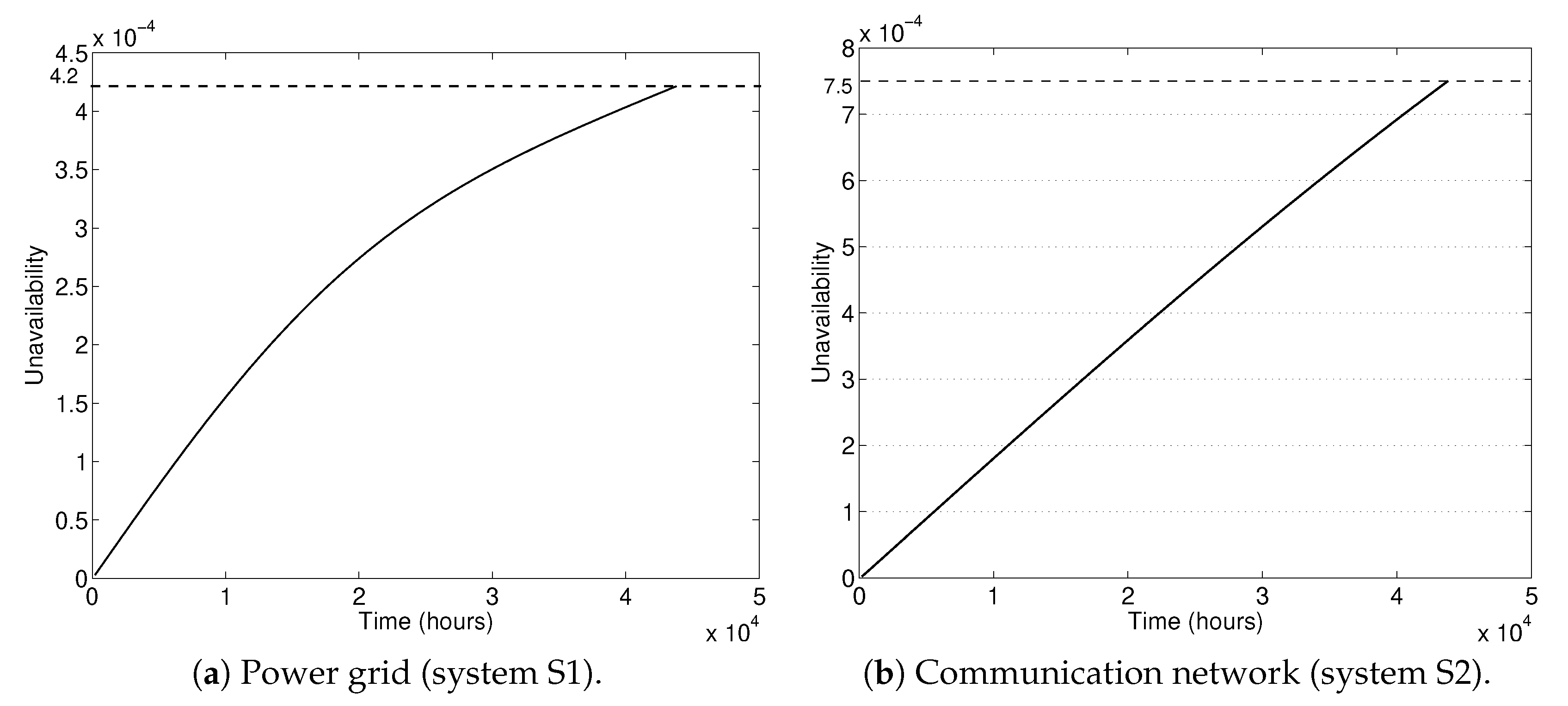
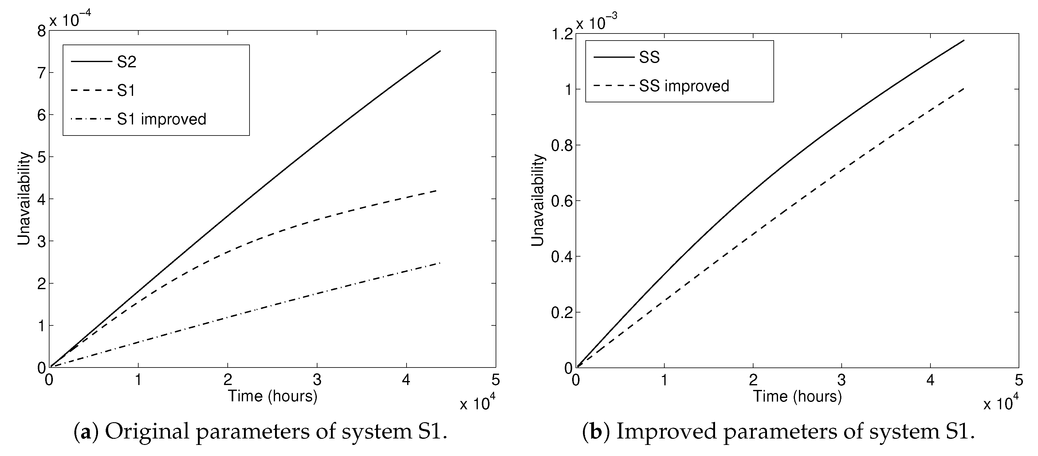
• Results indicated that the original design has an unacceptable large unavailability S1.
• Slightly modified design to improve the reliability of the interconnected system was proposed, in which only a limited number of components in the system were modified to keep the additional costs of the improved design limited.
• Numerical results indicated reduction in the unavailability of the improved interconnected system in comparison with the initial reliability design.
• The proposed unavailability exploration strategy is general and can bring a valuable reliability improvement in interconnected systems including the energy and communication sectors.

The aim of further research is to investigate the factors that contribute to communication equipment failures in electricity distribution systems and to quantify their relative importance. Specifically, the influence of environmental conditions, hardware and software failures, and communication disruptions that affect the reliability of the RTU will be investigated. A mathematical model will be developed to estimate the probability of failure of the RTU and assess the importance of each factor. The results of this study will provide valuable insights into the design and maintenance of distribution systems, which will contribute to increased reliability and reduced downtime.

References

1. Briš, R.; Byczanski, P. On innovative stochastic renewal process models for exact unavailability quantification of highly reliable systems. Proc. Inst. Mech. Eng. Part J. Risk Reliab. 2017, 231, 617–627. [Google Scholar] [CrossRef]
2. Ruijters, E.; Stoelinga, M. Fault tree analysis: A survey of the state-of-the-art in modeling, analysis and tools. Comput. Sci. Rev. 2015, 15, 29–62. [Google Scholar] [CrossRef]
3. Chen, Y.; Zhang, N.; Yan, J.; Zhu, G.; Min, G. Optimization of maintenance personnel dispatching strategy in smart grid. World Wide Web 2023, 26, 139–162. [Google Scholar] [CrossRef]
4. Nagaraju, V.; Fiondella, L.; Wandji, T. A survey of fault and attack tree modeling and analysis for cyber risk management. In Proceedings of the 2017 IEEE International Symposium on Technologies for Homeland Security (HST), Boston, MA, USA, 25–26 April 2017; pp. 1–6. [Google Scholar]
5. Garg, H.; Ram, M. Reliability Management and Engineering: Challenges and Future Trends; CRC Press: Boca Raton, FL, USA, 2020. [Google Scholar]
6. Pirbhulal, S.; Gkioulos, V.; Katsikas, S. A Systematic Literature Review on RAMS analysis for critical infrastructures protection. Int. J. Crit. Infrastruct. Prot. 2021, 33, 100427. [Google Scholar] [CrossRef]
7. Budde, C.E.; Stoelinga, M. Efficient algorithms for quantitative attack tree analysis. In Proceedings of the 2021 IEEE 34th Computer Security Foundations Symposium (CSF), Dubrovnik, Croatia, 21–24 June 2021; pp. 1–15. [Google Scholar]
8. Lazarova-Molnar, S.; Mohamed, N.; Shaker, H.R. Reliability modeling of cyber-physical systems: A holistic overview and challenges. In Proceedings of the 2017 Workshop on Modeling and Simulation of Cyber-Physical Energy Systems (MSCPES), Pittsburgh, PA, USA, 18–21 April 2017; pp. 1–6. [Google Scholar]
9. Niloofar, P.; Lazarova-Molnar, S. Data-driven extraction and analysis of repairable fault trees from time series data. Expert Syst. Appl. 2023, 215, 119345. [Google Scholar] [CrossRef]
10. Rehioui, H.; Idrissi, A. New clustering algorithms for twitter sentiment analysis. IEEE Syst. J. 2019, 14, 530–537. [Google Scholar] [CrossRef]
11. Baklouti, A.; Nguyen, N.; Choley, J.Y.; Mhenni, F.; Mlika, A. Free and open source fault tree analysis tools survey. In Proceedings of the 2017 Annual IEEE International Systems Conference (SysCon), Montreal, QU, Canada, 24–27 April 2017; pp. 1–8. [Google Scholar]
12. Rodrigues, M. Network Availability: How Much Do You Need? How Do You Get It? (Logic Monitor). 2023. Available online: https://www.cisco.com/site/au/en/solutions/full-stack-observability/index.html?team=digital_marketing&medium=paid_search&campaign=reimagine_applications&ccid=cc002659&dtid=psexsp001647&gad_source=1&gclid=EAIaIQobChMIlMTEjuyDgwMVmKpmAh0GNwabEAAYASAAEgLwn_D_BwE&gclsrc=aw.ds (accessed on 14 June 2023).
13. Zhang, R.; Zhao, Z.; Chen, X. An overall reliability and security assessment architecture for electric power communication network in smart grid. In Proceedings of the 2010 International Conference on Power System Technology, Hangzhou, China, 24–28 October 2010; pp. 1–6. [Google Scholar]
14. Cisco. Cisco Crosswork Cloud Trust Insights Data Sheet. 2021. (Data-Sheet). Available online: https://www.cisco.com/c/en/us/products/collateral/cloud-systems-management/crosswork-network-automation/datasheet-c78-741972.html (accessed on 6 July 2023).
15. Cisco. Network Availability: How Much Do You Need? How Do You Get It? (White Paper). 2004. Available online: https://www.cisco.com/web/IT/unified_channels/area_partner/cisco_powered_network/net_availability.pdf (accessed on 23 June 2023).
16. Xu, S.; Qian, Y.; Hu, R.Q. On reliability of smart grid neighborhood area networks. IEEE Access 2015, 3, 2352–2365. [Google Scholar] [CrossRef]
17. Drholec, J.; Gono, R. Reliability database of industrial local distribution system. In Proceedings of the First International Scientific Conference “Intelligent Information Technologies for Industry” (IITI’16); Springer: Berlin/Heidelberg, Germany, 2016; Volume 2, pp. 481–489. [Google Scholar]
18. Muhammad Ridzuan, M.I.; Djokic, S.Z. Energy regulator supply restoration time. Energies 2019, 12, 1051. [Google Scholar] [CrossRef]
19. Santos, G.L.; Endo, P.T.; Gonçalves, G.; Rosendo, D.; Gomes, D.; Kelner, J.; Sadok, D.; Mahloo, M. Analyzing the it subsystem failure impact on availability of cloud services. In Proceedings of the 2017 IEEE Symposium on Computers and Communications (ISCC), Heraklion, Greece, 3–6 July 2017; pp. 717–723. [Google Scholar]
20. Union, I.T. Series G: Transmission Systems and Media, Digital Systems and Networks. Passive Optical Network Protection Considerations (ITU-T, Series G—Supplement 51, 02/2016). 2016. Available online: https://www.itu.int/rec/dologin_pub.asp?lang=f&id=T-REC-G.Sup51-201602-S!!PDF-E&type=items (accessed on 16 July 2023).
21. Prat, J. Next-Generation FTTH Passive Optical Networks: Research towards Unlimited Bandwidth Access; Springer: Berlin/Heidelberg, Germany, 2008. [Google Scholar]
22. Verbrugge, S.; Colle, D.; Demeester, P.; Huelsermann, R.; Jaeger, M. General availability model for multilayer transport networks. In Proceedings of the 5th International Workshop on Design of Reliable Communication Networks, Ischia, Italy, 16–19 October 2005; p. 8. [Google Scholar]
23. Scheer, G.W. Answering substation automation questions through fault tree analysis. In Proceedings of the Fourth Annual Texas A&M Substation Automation Conference, College Station, TX, USA, 8–9 April 1998. [Google Scholar]
24. Dolezilek, D.J. Choosing between Communications Processors, RTUS, and PLCS as Substation Automation Controllers; White Paper; Schweitzer Engineering Laboratories, Inc.: Pullman, WD, USA, 2000. [Google Scholar]
25. Scholl, M.; Jain, R. Availability and Sensitivity Analysis of Smart Grid Components. 2011. Available online: https://www.cse.wustl.edu/~jain/cse567-11/ftp/grid/index.html (accessed on 26 June 2023).
26. Briš, R.; Byczanski, P.; Goňo, R.; Rusek, S. Discrete maintenance optimization of complex multi-component systems. Reliab. Eng. Syst. Saf. 2017, 168, 80–89. [Google Scholar] [CrossRef]
27. Vrtal, M.; Fujdiak, R.; Benedikt, J.; Topolanek, D.; Ptacek, M.; Toman, P.; Misurec, J.; Beloch, M.; Praks, P. Determination of Critical Parameters and Interdependencies of Infrastructure Elements in Smart Grids. In Proceedings of the 2023 23rd International Scientific Conference on Electric Power Engineering (EPE), Aalborg, Denmark, 4–8 September 2023; pp. 1–6. [Google Scholar]
28. Vrtal, M.; Benedikt, J.; Fujdiak, R.; Topolanek, D.; Toman, P.; Misurec, J. Investigating the Possibilities for Simulation of the Interconnected Electric Power and Communication Infrastructures. Processes 2022, 10, 2504. [Google Scholar] [CrossRef]
29. Bose, S.; Gayme, D.F.; Chandy, K.M.; Low, S.H. Quadratically constrained quadratic programs on acyclic graphs with application to power flow. IEEE Trans. Control Netw. Syst. 2015, 2, 278–287. [Google Scholar] [CrossRef]
30. Wang, D.; Zhou, F.; Li, J. Cloud-based parallel power flow calculation using resilient distributed datasets and directed acyclic graph. J. Mod. Power Syst. Clean Energy 2019, 7, 65–77. [Google Scholar] [CrossRef]
31. Jha, N.K. Low power system scheduling and synthesis. In Proceedings of the IEEE/ACM International Conference on Computer Aided Design (ICCAD 2001), IEEE/ACM Digest of Technical Papers (Cat. No. 01CH37281), San Jose, CA, USA, 4–8 November 2001; IEEE: Piscataway, NJ, USA, 2001; pp. 259–263. [Google Scholar]
32. Ding, S.; Cao, Y.; Vosoogh, M.; Sheikh, M.; Almagrabi, A. A directed acyclic graph based architecture for optimal operation and management of reconfigurable distribution systems with PEVs. IEEE Trans. Ind. Appl. 2020. [Google Scholar] [CrossRef]
33. Maharana, M.K.; Swarup, K.S. Particle swarm optimization based corrective strategy to alleviate overloads in power system. In Proceedings of the 2009 World Congress on Nature & Biologically Inspired Computing (NaBIC), Coimbatore, India, 9–11 December 2009; pp. 37–42. [Google Scholar]
34. Lohith, Y.; Narasimman, T.S.; Anand, S.; Hedge, M. Link peek: A link outage resilient ip packet forwarding mechanism for 6lowpan/rpl based low-power and lossy networks (llns). In Proceedings of the 2015 IEEE International Conference on Mobile Services, New York, NY, USA, 27 June–2 July 2015; pp. 65–72. [Google Scholar]
35. Allan, R.; De Oliveira, M.; Kozlowski, A.; Williams, G. Evaluating the reliability of electrical auxiliary systems in multi-unit generating stations. IEE Proc. (Gener. Transm. Distrib.) 1980, 127, 65–71. [Google Scholar] [CrossRef]
36. Stanek, E.K.; Venkata, S. Mine power system reliability. IEEE Trans. Ind. Appl. 1988, 24, 827–838. [Google Scholar] [CrossRef]
37. Farag, A.; Wang, C.; Cheng, T.; Zheng, G.; Du, Y.; Hu, L.; Palk, B.; Moon, M. Failure analysis of composite dielectric of power capacitors in distribution systems. IEEE Trans. Dielectr. Electr. Insul. 1998, 5, 583–588. [Google Scholar] [CrossRef]
38. Roos, F.; Lindah, S. Distribution system component failure rates and repair times—An overview. In Proceedings of the Nordic Distribution and Asset Management Conference, Espoo, Finland, 23 August–24 August 2004; pp. 23–24. [Google Scholar]
39. Anders, G.J.; Maciejewski, H.; Jesus, B.; Remtulla, F. A comprehensive study of outage rates of air blast breakers. IEEE Trans. Power Syst. 2006, 21, 202–210. [Google Scholar] [CrossRef]
40. He, Y. Study and Analysis of Distribution Equipment Reliability Data (Datastudier och Analys av Tillförlitlighetsdata på Komponentnivå för Eldistributionsnät). Elforsk Rapport 10:3, ELFORSK. 2010. Available online: https://docplayer.net/39290413-Study-and-analysis-of-distribution-equipment-reliability-data.html (accessed on 15 July 2023).
Figure 1. Considered representative interconnected infrastructures of power and communication networks in a Smart Grid domain.
Algorithms 16 00561 g001
Figure 2. Considered representative topology of the power distribution network.
Algorithms 16 00561 g002
Figure 3. Considered representative topology of the control and communication network part including the most common components.
Algorithms 16 00561 g003
Figure 4. Diagram of interconnected infrastructures simplified by omitting the elements without direct influence on the defined system function.
Algorithms 16 00561 g004
Figure 5. AG of the power grid part of the simplified test network.
Algorithms 16 00561 g005
Figure 6. AG of the communication network part of the simplified test network.
Algorithms 16 00561 g006
Figure 7. AG of the simplified interconnected test network.
Algorithms 16 00561 g007
Figure 8. Graphic display of the relationship between parameters MTBF, MTTRes, and MTTF.
Algorithms 16 00561 g008
Figure 9. Graphic display of the relationship between parameters MTTRes, MTTI, MTTK, MTTRep, and MTTV.
Algorithms 16 00561 g009
Figure 10. Unavailability evolution of the power grid (a) and the communication network (b) within the mission time of 5 years.
Algorithms 16 00561 g010
Figure 11. Comparison of unavailability evolution of systems SS, S1 and S2 for the case with original parameters.
Algorithms 16 00561 g011
Figure 12. Comparison of the unavailability evolution within the mission time of 5 years with original and improved parameters for Systems S1 and S2 (a) andSystem SS (b).
Algorithms 16 00561 g012