Abstract
Timely information about the need to thin forests is vital in forest management to maintain a healthy forest while maximizing income. Currently, very-high-spatial-resolution remote sensing data can provide crucial assistance to experts when evaluating the maturity of thinnings. Nevertheless, this task is still predominantly carried out in the field and demands extensive resources. This paper presents a deep convolutional neural network (DCNN) to detect the necessity and urgency of carrying out thinnings using only remote sensing data. The approach uses very-high-spatial-resolution RGB and near-infrared orthophotos; a canopy height model (CHM); a digital terrain model (DTM); the slope; and reference data, which, in this case, originate from spruce-dominated forests in the Austrian Alps. After tuning, the model achieves an F1 score of 82.23% on our test data, which indicates that the model is usable in a practical setting. We conclude that DCNNs are capable of detecting the need to carry out thinnings in forests. In contrast, attempts to assess the urgency of the need for thinnings with DCNNs proved to be unsuccessful. However, additional data, such as age or yield class, have the potential to improve the results. Our investigation into the influence of each individual input feature shows that orthophotos appear to contain the most relevant information for detecting the need for thinning. Moreover, we observe a gain in performance when adding the CHM and slope, whereas adding the DTM harms the model’s performance.
1. Introduction
Maintaining a healthy, stable forest to produce valuable wood requires fostering the forest. An essential technique to accomplish this is a silvicultural operation called thinning [1]. The main objective of thinning is to regulate the vertical space of trees, thus steering the allocation of the available resources (e.g., sunlight, water, and nutrients) into the stems of remaining higher-quality trees [2]. Although the primary objective of thinning is to prepare the forest stand for a final harvest, it also provides forest owners with the opportunity to obtain additional income by selling the removed trees [3,4,5,6].
Determining if a forest stand needs thinning is a complex task since it depends on many factors, such as soil quality and the composition of trees regarding age and species [7]. This makes assessing a forest stand for the necessity of thinning a non-trivial task, and this is why the job is still mainly conducted by specialized forest personnel. Sending personnel into the field is often very expensive. Hence, thinning assessments are either not performed at all, as in the case of small forest owners, or carried out at long time intervals. Long time intervals might be sufficient for slowly growing sites; however, vital areas with high mean annual increments are often overlooked, which results in the sub-optimal timing of thinning in these stands.
Recently, the proliferation of the amount of and improvement in the quality of remote sensing data have made it possible to acquire uniform and detailed aerial information over large areas [8]. Furthermore, with recent advances in sensor technology as well as computing power, there has been increased interest in applying algorithms for the automated extraction of forest parameters from remotely sensed spectral information [9]. Aerial forestry data coupled with recent increases in computing power allow machine learning (ML) algorithms to be deployed for applications such as detecting changes in forests [10,11], classifying tree species [12,13,14,15], and estimating stand volume [16,17,18].
Despite the high level of importance of the timely planning of forest operations, few studies have been conducted to predict the necessity of thinning from remote sensing data. There are only two known studies that addressed this challenge. First, ref. [19] tried to predict forest operations at the stand level using Landsat satellite imagery with moderate success. Then, ref. [20] employed ALS data-derived features to predict thinning maturity at the stand level. This study showed much better results, with classification accuracy ranging from 79% to 83% when predicting the timing of the subsequent thinning. Another approach to predicting the need for thinning is to utilize key forest parameters acquired through remote sensing, together with additional inventory data, to create statistical models [21]. Nevertheless, ALS data are still expensive to obtain, and only a few countries acquire it systematically.
We used semantic segmentation to extract information about the need for thinning from widespread areal images as this method was successfully used for many remote sensing tasks [22]. Semantic segmentation is a computer vision task where the algorithm labels each pixel or patch of an image according to a predefined range of classes. The utilization of end-to-end DCNNs for the task of semantic segmentation has increased greatly and was accelerated via the first end-to-end fully convolutional network (FCN) [23]. Since the invention of this network type, many different architectures have been proposed and adapted to remote sensing applications [24,25,26]. The main advantage of using DCNNs for semantic segmentation is their effectiveness in extracting complex features from wide receptive fields. Nonetheless, this capability comes with the price of not being able to maintain a high spatial resolution and results in inaccurate and blurred boundaries between the classes. To counteract this, newer DCNNs use more pronounced or distinct encoder–decoder architectures with skip connections. For example, UNet applies such skip connections in its symmetrical encoder–decoder architecture [27], where the features extracted in the encoder are directly coupled to the corresponding decoder layers. The outstanding performance of this architecture, together with its simplicity, has ensured its widespread adoption in the remote sensing research community for a variety of applications, such as ship detection [28], road extraction [29], and land cover classification [30].
Deeper DCNNs with more stacked layers were created to obtain models that can learn more complex input representations. However, these deeper DCNNs often resulted in worse-performing models than their more shallow predecessors due to the degradation problem [31]. This issue was resolved using deep residual networks (e.g., ResNet) that employed residual blocks, which added an identity shortcut connection and overcame the degradation problem [32]. The further development of DCNNs resulted in the creation of a network architecture called DenseNet, which utilizes dense blocks that introduce direct connections from any layer to all subsequent layers to further improve the flow of information between layers [33]. Jegou et al. [34] adopted the DenseNet connection structure for semantic segmentation by applying dense blocks to a UNet-like symmetric encoder–decoder structure. This merge resulted in a DCNN called FC-DenseNet, which required fewer input parameters while performing better on various semantic segmentation challenges.
Another compelling approach to resolving the trade-off between high-context extraction with heavy downsampling and accurate boundary prediction is the use of dilated or atrous convolutions. Atrous convolutions utilize a convolution filter that is spaced apart, thus allowing them to attain a wider field of view while retaining their spatial dimensions. Ref. [35] proposed a DCNN architecture called DeepLabv1 that incorporates atrous convolutions into a VGG-16 architecture to address the trade-off between high-context extraction and heavy downsampling. Several revisions to this architecture occurred, including, among other things, the incorporation of the spatial pyramidal pooling method that was introduced in SPPNet [36] and adopted by [37] to create the atrous spatial pyramid pooling (ASPP) method used in DeepLabv2. The current network architecture, DeepLabv3+ [38], provides some of the best results for semantic segmentation challenges. Furthermore, its use in remote sensing applications is auspicious. For example, ref. [39] showed the DeepLabv3+ network’s excellent performance in classifying marsh vegetation in China. Accordingly, DeepLabv3+ is the network used in Section 3.2 to classify regions in need of tree thinning.
Nevertheless, little research has been performed to detect the necessity of thinning solely with remote sensing data. This paper presents a model capable of achieving this task.
In this study, we tested a deep learning approach to determine if remote sensing data alone could be used to detect the need for thinning. The two factors investigated were whether the approach could
- Detect if thinning is needed, based on deep convolutional neural networks (DCNNs) trained on very high spatial resolution imagery;
- Differentiate between thinnings with different urgencies (i.e., timescales).
An accurate prediction of thinnings from remote sensing data has the potential to deliver information for vast or remote forest areas promptly, thus improving the stability and wood quality of forests.
2. Previous Research and Background
This section provides background information related to detecting the necessity of thinnings with the help of remote sensing. First, we introduce thinning, its effect on the forest stand, and its impact on the timber quality. After that, we show the current state of remote sensing in forestry on its most important research questions. Finally, we review the current state of the art on image change analysis techniques and their application in remote sensing.
2.1. Thinning
Thinning can be seen as the primary steering technique in preparation for the final harvest. Although many types of thinning have emerged throughout the history of forestry, the main objective of all of them is to remove some trees to accelerate growth in the remaining future crop trees. Notably, this enables the remaining trees to allocate the newly available resources mainly into their basal stem [2,40], which is economically the most valuable part of the tree.
Furthermore, by applying selective thinning, hence selecting the most promising future crop trees, the log quality can be significantly enhanced [41,42]. Thus, thinning provides an opportunity to increase the amount of good-quality timber in the final harvest while producing additional income from sales of the removed trees. Since the main objective of many forest owners is to maximize the net present value of their forest area, thinned stands outperform unmanaged stands [4,5,6].
One of the main concerns of performing thinning is the enhanced risk of damage to the forest due to high wind or snow. Various studies have shown that right after thinning, a forest stand’s stability is lower due to the higher roughness of the tree crowns [43]. Although this is true for the time right after thinning, the risk of injuries decreases with time until no additional risk is present anymore [43,44]. Nonetheless, thinning in Norway spruce stands has been recorded to reduce the h/d ratio of trees (height-to-diameter ratio) [45]. The h/d ratio is an indicator for the individual stability of a tree, where low h/d values are equivalent to high tree stability [46,47,48]. Thus, newer research suggests that early heavy thinning might even increase the stability of a stand [49]. Therefore, timeliness is crucial, as delaying thinnings results in an increased risk of damage to the stands [46,50].
Optimal thinning schemes differ by the tree species, any previously applied measures, and the density of the standing trees. Due to these variations, it is essential to define the type of thinning that is being used throughout this study. The study area is predominantly stocked with Norway spruce-dominated coniferous forest. The researchers in [51] and, then later, those in [6] found that the highest economic return on investment is produced via selective crown thinning with a selection of target trees for this typical forest type. The Austrian Federal Forest adopted this thinning type as the standard thinning scheme, and thus, nearly all thinnings are planned as such. Therefore, when we refer to thinning in this study, it is equivalent to this specific thinning type.
Thinnings of Norway Spruce stands of the Austrian Federal Forest are executed 2–3 times during the lifetime of a stand, where 1/4 to 1/3 of the actual stocking volume is harvested each time. The first thinning is carried out typically at around 13–19 m top height, followed by a second thinning at approximately 20–30 m top height, with a third thinning at good-growing sites. The exact timing of the procedure depends on the density of the standing trees, which is related to conditions such as the timing of the previous thinning and the growth performance at the site.
2.2. Remote Sensing in Forestry
Utilizing remote sensing imagery for extracting information about the forest structure and its employment in forest planning has been practiced since the 1960s [52]. Remote sensing provides the opportunity to gather uniform information about larger areas otherwise impossible to collect from field measurements. The automated derivation of crucial information from the forest, such as tree species classification and wood volume estimation, has long been a goal of researchers in forestry [53]. Traditionally, collecting information about the forest structure was based on sending experts into the field for conventional forest inventories. This process is costly and often not affordable for small forest owners. With the advances in sensor technology as well as computing power, the interest in applying algorithms for the automated extraction of forest parameters from remotely sensed spectral information has increased [9].
At present, the leading sensing instrument technologies applied for retrieving forestry-relevant metrics are multi-spectral or hyperspectral cameras; light detection and ranging (lidar); and to a certain extent, synthetic-aperture radars (SAR) [54]. These instruments can be mounted on three different platforms—satellites, aircrafts, and unmanned aerial vehicles (UAVs)—each giving the sensing instrument different ranges of spatial resolution. Moreover, sensors mounted on a plane can support conventional forest inventories and provide helpful information for operational forest management [53,55].
Despite the importance of forest operations such as thinning, few studies have tried to create models that can predict the necessity of thinning directly from remote sensing data [20]. Most research has focused on change detection, tree species classification, as well as wood volume estimation. Although substantial progress has been made in all the introduced research questions, they are far from being solved and are still active research subjects.
2.3. Change Analysis in Forest Management
A forest changes continuously, whether as a result of forest operations such as thinning or clear-cutting or due to forest damage caused by heavy winds, fire, and other natural disasters. The human-made changes can be reported and easily updated. However, changes induced by nature must be spotted differently. The automatic detection of changes in the forest using aerial imagery shows promising results in areas where severe changes have happened, such as clear-cutting and intense storm damage. However, moderate changes such as thinning are much harder to discover [10]. When using airborne laser scanning (ALS) as the data source to detect changes, Yu et al. [11] were able to identify the removal of individual trees. Nonetheless, acquiring aerial images or even more expensive ALS data is often performed at considerable intervals. Hence, a more interesting remote sensing platform for this problem is satellites. Due to their higher temporal resolution, satellites can provide much more timely data, as is often required in disaster response. In particular, SAR data can provide data even on overcast days. Although weather conditions influence the signal, this noise can be filtered, as [56] demonstrated, and therefore were able to detect changes in forest areas greater than 1 ha with Sentinel-1 data.
3. Materials and Methods
3.1. Materials
For training the machine learning model, we used data collected for the Lungau region through aerial imagery, airborne laser scanning (ALS), as well as data from forest management plans. These data were first cleaned and preprocessed before being used as input data for the machine learning algorithms, resulting in 5 distinct input types, as summarized in Table 1. This section defines what kind of thinning is used in this study and describes the data and its acquisition, and the data preprocessing.

Table 1.
Data sources. NIR: near-infrared, CHM: canopy height model, DTM: digital train model, AI: aerial imagery, ALS: airborne laser scanning, RD: actual thinning reference data, Res.: spatial resolution, S.E.: standard error, and Year: acquisition year. Slope data computed from the DTM.
3.1.1. Study Area
Located in the Lungau region (Tamsweg district), Austria (47°00′–47°13′ N, 13°23′–14°00′ E, UTM/WGS84 projection), the study area is managed by the Austrian Federal Forests (ÖBF AG). Part of the Central Eastern Alps, the area is mountainous with an altitude range of 993–1906 m and has a distinct alpine climate with an average annual temperature of 5.2 C, mean annual precipitation ranging between 770 and 840 mm, and a snow cover minimum of 1 cm for 105 days per year. The study area, illustrated in Figure 1, has an area of 21,826.55 ha and is predominantly covered with forests (63.9% of the area). The forest area is further divided into commercial forests and protective forests. The commercial forest is managed to maximize the income from timber production while minimizing the risk of forest damage. In contrast, a protective forest’s objective is to protect against avalanches, rockfall, erosion, and floods. Although thinnings are planned in both forest types, thinnings in the protective forest aim to ensure its protective function, whereas thinnings, as specified in Section 2.1, are just planned in a commercial forest. In this paper, we are interested in the forests where commercial thinnings are feasible. Hence, we restrict the study area to the commercial forest. The commercial forest has an extent of 9353.54 ha and is stocked with mainly coniferous forests. The most frequent tree species are 81.0% Norway spruce (Picea abies, 81.0%) and European larch (Larix decidua, 17.6%). The remaining 1.4% of the area is stocked with deciduous forests.
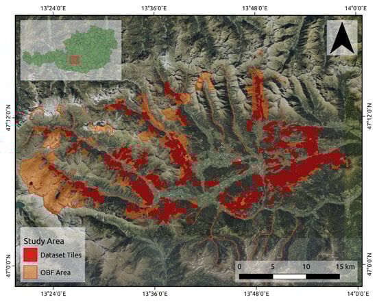
Figure 1.
Study area of Lungau, Austria. The Austrian Federal Forest area is colored in orange and includes commercial and protective forest as well as non-forest areas. Shown in red are the tiles that are used to create the dataset that is used in this paper. The background image is a true-color orthophoto from airborne photography [57] of the region in Austria that was used. The region in the main image is the same as the red square shown in the full map of Austria shown in the upper left.
3.1.2. Remote Sensing and Ground Truth Data Acquisition
As shown in Table 1, all data came from three sources and were acquired at three disparate points in time. Ideally, all data should be acquired simultaneously, but we were limited in this study.
The aerial imagery was acquired by the States of Austria, where one-third of Austria was updated every year. All aerial imagery for the study site was recorded on 11 September 2018 and 12 September 2018 with an UltraCam Eagle Mark 3 431S61680X916102-f100 mounted on a Beechcraft Super King Air B200 D-IWAW. Four bands were acquired with a spatial resolution of 20 cm: three bands for RGB and one band in the near-infrared (NIR) spectrum (Table 1). After acquisition, the raw data were geometrically and radiometrically corrected with the corresponding calibration data of the camera, and the four channels were stitched together using the monolithic stitching method [58]. The second product that was derived from the aerial photos is the canopy height model (CHM). To obtain the CHM, first, the digital surface model (DSM) was calculated using photogrammetry from overlapping air images. Then, the CHM was calculated by subtracting the DSM from the DTM. For this study, the Federal Forest Office (BFW) calculated the CHM.
Acquisition of the utilized digital terrain model (DTM) was performed via airborne laser scanning (ALS) in 2013 as part of the EU project INTERREG. The slope was calculated from the DTM using the Horn algorithm [59]. The Austrian Federal Forests provided all data.
Reference data collection was performed by forest engineers from May 2017 until November 2017 and subsequently digitalized by April 2018. This data acquisition was carried out as part of the forest management plan update by the Austrian Federal Forests. Forest engineers assessed every forest stand by measuring the basal area and tree heights to derive the most important key figures such as tree species composition, yield class, and stocking volume. Another part of the assessment was the planning of thinnings that need to be executed to ensure optimal growth of the trees and to maintain healthy forest stands with high-quality wood. At the Austrian Federal Forests, thinnings are planned in three urgency levels, i.e., the forest stand:
- Urgency 1—needs thinning during the next 0 to 3 years;
- Urgency 2—needs thinning during the next 3 to 10 years;
- Urgency 3—can be thinned after 10 years or can be postponed until the next management plan.
The terminology ’urgency level’ is an internal annotation used by the Austrian Federal Forests as a practical approach to recording the urgency of use by a forest manager. However, just the first two (urgency 1 and urgency 2) are relevant, since by the time urgency 3 would be executed, a new management plan will have been made. Therefore, it is used very rarely and will not be considered in this study. The acquired data were populated into a database (See Table 2), and the spatial information about the forest stands was drawn in a GIS. Subsequently, both data sources were spatially registered.
Table 2.
Reference data classes, their definitions, and occupied area.
3.2. Methods
The goal is to predict where and when thinnings are necessary. Deep convolutional neural networks (DCNNs) are used for classification based on pixels, i.e., semantic segmentation. This section describes the data preprocessing, outlines the experimental design, describes the training procedure, and presents the applied evaluation criteria.
3.2.1. Data Preprocessing
Due to different spatial and temporal resolutions (Table 1), the described data needed preprocessing before input into the DCNN. The workflow is shown in Figure 2 and described in this section in more detail.
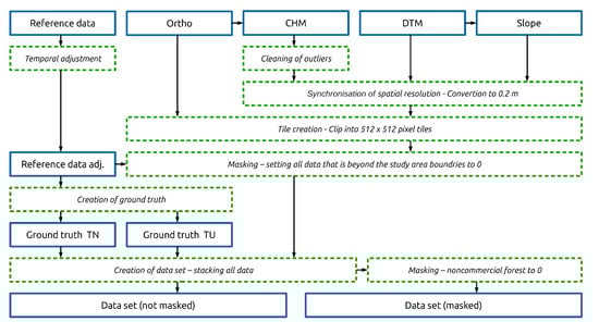
Figure 2.
Data preprocessing workflow with all data manipulation steps (see text).
The provided canopy height model (CHM) contained values ranging from −73.9 to 138. Since values below 0 are physically impossible and tree heights above 45 m are improbable in Austria, these values need adjustment. Therefore, values below 0 and over 40 m were highlighted, visually inspected, and classified in GIS. The analysis showed that highlighted pixels higher than 47 m and negative values were predominantly rocky steep slopes. Consequently, all pixels with a value below 0 and above 47 m were set to 0.
3.2.2. Synchronization of Spatial Resolution
Next, the spatial resolution of all input data was synchronized. As shown in Table 1, the orthophotos have a spatial resolution of 0.2 m as opposed to all other raster data having a spatial resolution of 1 m. There are benefits and drawbacks to using either as the standard spatial resolution. Using 0.2 m as the standard results in more detail in the four orthophoto layers. Greater detail can be beneficial for the deep learning algorithm to recognize individual tree crowns and thus helps it determine the density of the forest. In contrast, the resolution of 1 m would provide a broader field of view when maintaining the same input image size as that in the DCNN. The resolution of 0.2 m was chosen as the standard for all input data as, otherwise, the anticipated information loss would be too high. This assumption is based on the fact that the average tree crown diameter for a first thinning is approximately 2.5 m. Consequently, a pixel size of 1 m would imply that one tree crown is represented by about 3 pixels in contrast to the 13 pixels with a pixel size of 0.2 m. The determination of an individual tree crown using a 3-pixel resolution is much harder compared with a tree crown represented by 13 pixels. Consequently, all data with a spatial resolution of 1 m were converted using the GDAL library [60].
3.2.3. Tile Size
The data needed to be clipped into square tiles as it is the input type of the neural networks used in this study. Accordingly, an image size of 512 × 512 pixels was a favorable choice due to the possibility of processing this image size with modern GPUs with a decent batch size while maintaining a large field of view. Ultimately, the image size could be easily reduced by quartering the dataset without considerable effort, thereby increasing the batch size while processing accordingly. The image size of 512 × 512 pixels corresponds to 102.5 m × 102.5 m. Since one adult tree crown (Norway spruce) has a diameter of 5–6 m, 300–400 adult tree crowns can be represented on one tile.
3.2.4. Tile Creation
Only commercial forests are relevant for this study, since thinnings are only regularly planned and executed with commercial forests, as described in Section 2.1. Thus, a regular grid of 102.5 m × 102.5 m polygons was laid over the entire study area to create polygons that were then intersected with the reference data. Only polygons that contained over 25% commercial forest area were selected, while the remaining polygons were removed. Finally, the remaining polygons were used to clip all input raster data into 512 × 512 pixels tiles.
3.2.5. Reference Data Adjustment
Considering that the aerial imagery acquisition was recorded in September 2018 and the reference data were recorded from May to November 2017, the provided reference data needed to be adjusted. In the year between the two acquisitions, the study area was modified via planned and salvage logging [61]. This inconsistency was resolved using data from the Austrian Federal Forests database, where all cuttings are registered, to identify already carried out thinnings and salvage logging. Additionally, all commercial forest stands were visually inspected in GIS, and any noticeable errors were corrected.
3.2.6. Masking
Since the reference data are restricted to the study area and square tiles were used, part of the tile frequently contains no reference data (ground truth). Having parts of the tile with no ground truth information while orthophoto and DTM data are available would be misleading for the machine learning algorithm. Hence, all data outside the study area’s boundaries were removed. A binary mask from the reference data for every tile was created. In the resulting tiles, all information beyond the boundaries of the study area was set to 0.
3.2.7. Design of Ground Truth Label Models
The ground truth was created from the reference data with its six unique classes, as shown in Table 3. ’Void’ represents the absence of information, as described in Section 3.2.6. The other five classes are defined in Section 3.1.2, with three related to thinning. The first claim is that detecting forests that need thinning from remote sensing data is feasible. Since we are not interested in the urgency of the thinnings for this objective, we summarized thinning 1 and thinning 2 into one class called thinning. This ground truth is called TN (thinning necessity), and it differentiates between the classes void, thinning, no thinning, and other (Table 3). To address the second claim regarding the urgency of thinnings, we created another ground truth named TU (thinning urgency) (Table 3). TU was designed to differentiate between urgent thinning (thinning 1), not urgent thinning (thinning 2), no thinning, other, and void. Furthermore, we constructed two additional ground truths named masked TN and masked TU to focus exclusively on commercial forest (Table 4). The ground truths masked TN and masked TU expect to answer the claims as stated above for TN and TU; however all non-commercial forests (mainly protective forest and roads) were excluded. Finally, all ground truth data were created by rasterizing the reference data (vector data) with the GDAL library into images of the size 512 × 512 × 1.
Table 3.
Allocation of the reference data to ground truths TN and TU as well as the proportions of pixels representing each class. TN is an abbreviation for thinning necessity and TU for thinning urgency. The definitions of the reference data classes are explained in Table 2.
Table 4.
Allocation of the reference data to masked ground truths masked TN, masked TU, as well as the proportions of pixels representing each class. TN is an abbreviation for thinning necessity and TU for thinning urgency. The definitions of the reference data classes are explained in Table 2.
3.2.8. Creation of the Dataset
All the preprocessed input data and the generated ground truths were stacked into two datasets. Two separate datasets were needed since the input data corresponding to ground truths TN and TU were masked differently compared with the input data of ground truths masked TN and masked TU. Hence, the datasets stacked all preprocessed data into two hdf5 files. Each file consists of all tiles created inside the study area, as shown in Figure 1. Every tile is composed of the orthophoto (RGB+NIR, 4 layers), the CHM (1 layer), the DTM (1 layer), the slope (1 layer), and the ground truths (3 layers), thus adding up to 10 layers (Figure 3). Thus, in total, per dataset, 10,250 tiles were created, each of the size 512 × 512 × 10 pixels resulting in an array with the dimensions 10,250 × 10 × 512 × 512. All input data were standardized by subtracting the mean and dividing by the standard deviation for each value of each input channel (Table 1).
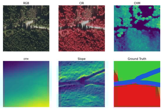
Figure 3.
Input data tile as used in the final dataset (non-masked). RGB: true color orthophoto, CIR: the color infrared orthophoto, CHM: crown height model, DTM: digital train model, Slope: slope and Ground Truth: ground truth TN. Ground truth classes are colored as follows: green represents forests not to be thinned (class: forest), red represents forest thinning is necessary (class: thinning), and blue represents everything else (class: other).
4. Results
4.1. Experimental Design
The experimental design can be divided into three major parts and is illustrated in Figure 4. In the first part (Section 4.4.1), a search for the best-performing DCNN architecture is performed. Then, the results of the models predicting the necessity of thinning (Section 4.4.3) and the urgency of thinning (Section 4.4.4) are analyzed. Finally, an ablation study (Section 4.4.5) is performed to determine the impact of the various input data sources.
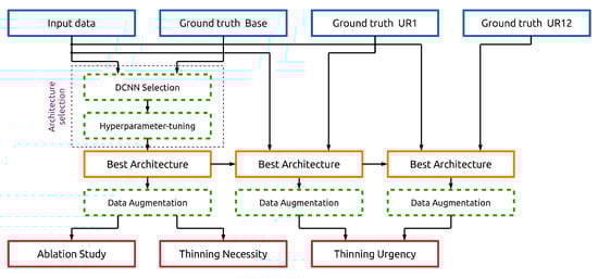
Figure 4.
Model training workflow with all processing steps to obtain the final models. The first stage is the architecture selection to find the best-performing DCNN architecture. The second stage is the training of the final models to answer the research objectives (thinning necessity, thinning urgency, and ablation study).
The exploration to find the best-performing DCNN architecture was conducted exclusively on the dataset with the ground truth TN (Table 3). The other ground truth types, with TU used later to clarify if deep nets can determine thinning urgency, was not employed in searching for the best model. From the literature review reported in [62], the following three DCNNs were found as the most promising architectures for solving the semantic segmentation problem:
- UNet [27];
- FC-DenseNet [34];
- DeepLabv3+ [38].
The architecture utilized in this study is shown in Figure A1. The DCNN was modified to accept the tiles from the dataset with the dimensions 512 × 512 × 7 as input and to output the predictions as a 512 × 512 × 1 array. We searched for the optimal architecture by evaluating the DCNNs on the dataset (TN). The DCNN achieving the best result was then chosen for further optimization experiments. This optimization consists of manipulating individual parts of the architecture to further optimize the model’s performance by applying the Bayesian optimization method [63]. This method is an alternative to an exhaustive full grid search, which is computationally expensive. Instead, it more efficiently searches for optimal hyper-parameters. In practice, we sequentially altered critical structures in the DCNN architecture and always adopted the structure that provided the best results. All DCNNs were implemented in PyTorch, and all supplementary code was written in Python. All code is freely available at https://github.com/satlawa/edin_thinning_necessity (accessed on 19 August 2023). The experiments were performed on a system with Ubuntu 20.04 as the operating system equipped with an I7 6700K CPU, 32GB of RAM, and an Nvidia RTX 3090.
After finding the best architecture, the final models were trained on the two datasets with all four ground truths (TN, TU, masked TN, and masked TU). These final models were then evaluated on the test set to estimate the actual performance on unseen data. Subsequently, the results were analyzed to determine whether the models could satisfactorily fulfill the intended task. In the case of the ground truths TN and masked TN, we examined if the necessity of thinnings can be detected via a DCNN using solely remote sensing data. Furthermore, the ground truths TU and masked TU were used to investigate if the urgency of thinnings can be determined in addition to detecting the necessity of thinnings.
Finally, an ablation study was performed by omitting different types of data from the input dataset with ground truth TN. The primary purpose of this experiment was to determine the importance of the individual input data types, as shown in Table 1.
4.2. Training
The dataset was randomly shuffled with 70% of the data used for training, 10% used for validation, and the remaining 20% used for testing of all models. The test set is exclusively applied to the best-performing model chosen via evaluation on the validation set.
After setting aside 20% of the data for the test set and 10% for validation, the remaining 70% of the data were randomly shuffled to train the model. All models were trained from scratch due to the dissimilarity of the input data compared with the datasets used on the pre-trained models. For the initialization of the weights, the Kaiming uniform initialization was employed [64]. For all experiments, the Adam optimizer was used as in [65], with an initial learning rate of (1) 0.01 for UNet, (2) 0.003 for FC-DenseNet, and (3) 0.001 for DeepLabv3+. After every epoch, a decay rate of 0.995 was applied to the learning rate. Since loss functions play a decisive role in training models, choosing a suitable loss function is essential [66]. Here, the distribution of the classes is skewed. Therefore, the DICE loss was used as the loss function. The DICE loss is defined as 1 − score (defined in Equation (5)). The batch size was chosen to be as large as possible, with the constraint being the memory of the GPU. Depending on the DCNN architecture, the batch size ranged between 16 and 72. However, due to long training times (up to 40 min for one epoch), only one five-fold cross-validation was carried out on the model TN. All models were trained until convergence, which required at least 50 epochs. Data augmentation in the form of horizontal flips was performed only on the training set and the previously chosen best-performing architecture. Data augmentation was restricted to horizontal flips due to the different environmental conditions on north- and south-facing slopes.
4.3. Evaluation Criteria
To evaluate the performance of the trained models thoroughly, five evaluation metrics were used. The first criterion is the overall accuracy (Acc), which is determined by dividing the number of all correctly classified pixels by the total number of pixels (Equation (1)).
where n is the number of images; and are the number of correctly labeled pixels in image i; and is the number of pixels in image i.
Although Acc is a very intuitive and thus common evaluation criterion, it is not very meaningful in cases where the distribution of classes is highly skewed, as is the case with the dataset we utilize (Table 2). Therefore, the metrics precision (Equation (3)), recall (Equation (2)), IoU (Equation (4)), and score (Equation (5)) are used for each class j:
where n is the number of images; is the number of pixels in image i that are correctly predicted as class j; is the number of pixels in image i that are incorrectly predicted as class j; and is the number of pixels in image i that are incorrectly predicted as any class other than class j.
Since this is a multi-class problem statement, we first calculate the proposed metrics per class and then determine the mean among all classes.
Despite providing all the above metrics for a holistic evaluation of the models, the score is used as the sole decisive evaluation score. Furthermore, the class void carries essentially no information. However, it is still necessary as the data outside the study area boundaries of the commercial forest boundaries (in the case of masked ground truths) must be represented. Nonetheless, although the class void is required for training the DCNNs, it is omitted in the presentation of the results as it was nearly perfectly classified and carried no valuable information. Moreover, its presence in the metrics would distort the results and indicate a better model performance than the particular model can achieve in reality.
4.4. Main Experimental Results
This section outlines and interprets the results of the performed experiments based on the previously described methods in Section 3.2. In particular, it presents the selection of the best-performing model. In addition, it demonstrates the feasibility of using DCNN for classifying the necessity and urgency of thinnings as well as the ablation study.
4.4.1. Architecture Selection
DCNN Selection
First, the performance of the three DCNN architectures is compared: UNet (), FC-DenseNet (), and DeepLabv3+ () on the dataset. DeepLabv3+ was chosen as the default network architecture, and the hyper-parameter tuning was performed on this DCNN. More details on the selection process can be seen in [62].
Hyper-Parameter Tuning
Although the DeepLabv3+ architecture is already pre-trained on the PASCAL VOC 2012 dataset, the dataset used here is considerably divergent. Thus, the hyper-parameters were optimized by applying the Bayesian optimization method [63]. The performance of the DCNN was explored by modifying five critical parts (abcde) of the DeepLabv3+, as shown in Figure 5.
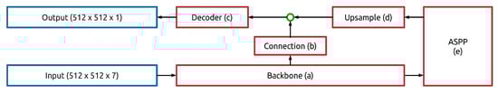
Figure 5.
Modified parts of DeepLabv3+. Parts are represented by letters abcde and are discussed in the main text.
The optimization process began with exchanging the modified Xception architecture with the Resnet 101 architecture as the backbone module of the DCNN (part a). This module is responsible for encoding the features from the initial images until they are passed to the ASPP module. As Table 5 shows, replacing the backbone module to the Resnet 101 architecture results in an score of 81.26%, which is a 0.88% gain compared with the 80.38% achieved with the Xception architecture. Hence, Resnet 101 was chosen as the backbone for the DeepLabv3+ net for all further experiments.
Table 5.
Effect of backbone (part a) choice on the validation set performance (ground truth TN). Acc: overall accuracy, mIoU: mean intersection over union, and F1: score.
Other variations were explored: using part b, ([1 × 1.48] convolution), part c ([1 × 1.256] × 2 upsample), part d, ([3 × 3.256] × 2 decoder), and part e (output stride 8) and augmentation with left–right flipping. Only the stride change and flipping gave an improvement, resulting in . More details of the tuning can be found in [62]. The best-performing hyper-parameters and DCNN architecture were used to train all subsequent models. A detailed diagram of the final architecture is provided in Appendix A.
4.4.2. Thinning
After optimizing the DCNN architecture on the dataset, the main research objectives of this study were addressed. First, the possibility of detecting the need for thinning with the optimized DCNN was evaluated, exclusively with remote sensing data (Section 4.4.3). Then, the feasibility of detecting the urgency for thinning was assessed (Section 4.4.4).
4.4.3. Thinning Necessity
Based on the network architecture from Section 4.4.1, the model was evaluated on the TN test set (Table 6). With a mean score of 82.23%, the model achieves a similar score to the 83.01% on the TN validation set. Thus, one can conclude that the chosen model is not overfitting the validation set. Additionally, when focusing on the class-specific scores, the model performs best on predicting the class no thinning, whereas the scores of the other two classes are significantly lower.
Table 6.
Classification scores and mean classification scores on the test set (ground truth TN) with five-fold cross-validation. The model’s objective is to detect the necessity of thinning. Classification definitions, thinning: thinning within 1–10 years, no thinning: no thinning necessary, other: non-forest areas. std: standard deviation.
When examining the confusion matrix in Table 7, one can gain further insight into the misclassifications of the model. Accordingly, the main mistakes are those between the classes thinning and no thinning as well as those between no thinning and other, while misclassifications between the classes thinning and other are insignificant. These results match our knowledge about the classes. Examples of predictions are illustrated in Figure 6.
Table 7.
Confusion matrix on the test set (ground truth TN). The numbers represent classified pixel times .
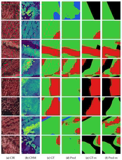
Figure 6.
Examples of semantic segmentation on the thinning necessity experiment test set. Columns: (a) CIR is false color composites with near-infrared, (b) CHM is the canopy height model, (c) GT is the ground truth of the thinning necessity set TN, (d) is the prediction of the model trained on the ground truth TN, (e) GT-m is the ground truth masked TN, and (f) is the prediction of the model trained on the ground truth masked TN. In (b), the color palette illustrates low heights as dark (dark blue) and high heights as bright (yellow). The colored pixels in (c–f) represent the following classes: black, void; red, thinning; green, no thinning; and blue, other.
For instance, class thinning represents dense forest with a minimum top height of around 13 m and thus contrasts to class other that often represents no vegetation or shallow growing vegetation like grassland or mountain pines. In contrast, it makes sense to see the model misclassifying the class no thinning with both other classes as it embodies forest at all ages. For example, a very young forest has almost identical features compared to grassland, as presented in Figure 6 row 1. Therefore, it is challenging and sometimes impossible to distinguish between no thinning and other with only remote sensing data. Equally ambitious are some classification cases between the classes thinning and no thinning. In this situation, the model struggles to differentiate between edge cases of dense forest (Figure 6 rows 5 to 8). These errors might arise due to a lack of information about the yield class of the forest. For instance, a dense old forest on less vigorous sites might appear similar to a dense middle-aged forest on productive sites or vice versa (Figure 6 row 6). Likewise, young forest on very viable sites might already require thinning during the planning period whereas a similar forest on less viable sites grows slower and should therefore not be planned for thinning.
Unquestionably, the model produces misclassifications, yet the results are excellent for most cases. For example, it correctly classifies the recently thinned forest as not to be thinned (Figure 6 row 2). Similarly, the model has no problems classifying correctly the cut forest and the more sparsely standing forest as no thinning, whereas the dense forest it accurately predicts as thinning (Figure 6 row 3 and 4).
As foresters are particularly interested in the differentiation between forest with and without the necessity of thinning, another model was trained that discriminates just among the classes thinning and no thinning. For this experiment, the dataset containing the ground truth masked TN was used, which just contains information about commercial forests while all other data was masked.
As reported in Table 8, a mean score of 85.32% was obtained. Hence, by focusing on merely two classes, the mean score was raised by 2.85% compared to the dataset without masking (Table 6). When concentrating on the class-specific scores, it can be seen that the mean score’s gain is due to the more accurate classification of the class thinning.
Table 8.
Classification scores and mean classification scores on the test set (ground truth masked TN). The model’s objective is to detect the necessity of thinning restricted to the commercial forest.
More detailed information about the misclassifications between the classes thinning and no thinning is provided in the confusion matrix in Table 9. What is striking is the lower number of categorized pixels due to the masking of non-commercial forest areas and the much higher number of false positives compared to the false negatives. This finding contrasts with the first model evaluated (Table 7), where the false positives and the false negatives were relatively balanced. Precisely this behavioral distinction can be observed in the examples of Figure 6. Particularly apparent is the difference in sensitivity in the fifth row of Figure 6, where the prediction of the non-masked dataset (Figure 6 column d) predicts no thinning on the entire tile while the prediction of the masked dataset (Figure 6 column f) classifies the entire commercial forest as in need of thinning.
Table 9.
Confusion matrix on test set (ground truth masked TN). The numbers represent classified pixels times .
4.4.4. Thinning Urgency
The next research question addressed is whether it is possible to detect the need for thinnings and predict their urgency accurately. Compared to the model in Section 4.4.3, this question adds another layer of complexity to the network since it has to assess the thinnings urgency. To answer this question, the ground truth masked TU was used. The idea of ground truth TU is to predict thinnings and their urgency directly. Hence it differentiates between very urgent thinnings (masked thinning 1), less urgent thinnings (masked thinning 2) and no need for thinning masked no thinning. A detailed description of the ground truths is provided in Section 3.2.7. Only the masked version is considered here to focus on the commercial forest. Experiments with the full data can be seen in [62].
Constraining the problem by just taking into account commercial forest increased the performance slightly in the case of ground truth masked TN (Section 4.4.3). Accordingly, the same strategy was applied to the model masked TU. However, the results show no significant overall improvement in the mean (Table 10) over model TU. Although the model masked TU achieves a higher score in class thinning 1 (51.48%) compared to model TU (41.03%), all other class scores achieve worse performance. Since we are particularly interested in predicting the urgency of thinning, model masked TU provides a slightly better alternative than model TU. Thus one can conclude that the restricted model masked TU gives a small improvement in class thinning 1 compared to the model TU. Figure 7f shows examples of the semantic segmentation results from the thinning urgency experiment. It is clear that the distinction between the two thinning classes (colors red and yellow) is not always very accurate.
Table 10.
Classification scores and mean classification scores on the test set (ground truth masked TU). The model’s objective is to detect the urgency of thinnings restricted to the commercial forest.
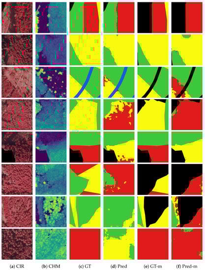
Figure 7.
Examples of semantic segmentation on thinning urgency test set. Column (a) CIR are false color composites with near-infrared, (b) CHM is the canopy height model, (c) GT is the ground truth thinning urgency set TU, (d) is the prediction of the model trained on the ground truth TU, (e) GT-m is the ground truth masked TU, (f) is the prediction of the model trained on the ground truth masked TU. In (b) the color palette illustrates low heights as dark (dark blue) and high heights as bright (yellow). The colored pixels in (c–f) represent the following classes, black: void, red: thinning 1, yellow = thinning 2, green: no thinning, blue: other.
Fortunately, perfect accuracy is not needed because the forestry management procedures can tolerate the slight inefficiency of postponing an urgent thinning until the next thinning review cycle.
4.4.5. Ablation Study
An ablation study investigated the importance of individual input features by training models with various combinations of removed input features. The factors explored were the inclusion or exclusion of these data planes: orthophoto, CHM (crown height model), DTM (digital train model), and slope. The performance variations of the different models provide insight into what effect a specific input feature has on the model. See [62] for the full details of the experiments summarized below.
The results showed that the inclusion of the DTM has little or a slightly negative impact on the model’s performance. When examining the classification scores, it is primarily in the class other where the inclusion of DTM deteriorates the performance. The input feature slope improves performance relative to models that do not contain it. Since slope is calculated from the DTM, we expected that the DCNN could at least partially learn to extract some useful information out of the DTM. However, it seems the DCNN is not capable of deriving slope out of the DTM. Possibly, this is because the input features slope and DTM provide only information about the terrain and not about the forest itself.
Omitting the input feature CHM results in models with a lower score compared with the equivalent models with CHM included, one can conclude that CHM contains some unique information since tree heights are essential criteria for assessing the necessity of thinning, as Section 2.1 briefly outlines.
Omitting the input feature orthophotos gives a significant decline in performance compared with the full model. It appears that orthophotos contains the most valuable information of all input features. This result coincides with the finding that the input feature orthophotos is also the most informative for human forest managers when assessing a forest.
5. Discussion
Timely planning and execution of thinnings are crucial for maintaining a healthy forest, but minimal research has been performed to derive the need for thinning directly from remote sensing data. Compared with detecting the necessity of thinnings, the estimation of inventory data [16,17,18] or the classification tree species [12,13,14,15] has received much more attention. Accordingly, this study demonstrates the potential of predicting the necessity of thinning with state-of-the-art deep learning architectures solely from high-altitude remote sensing data.
Using multispectral orthophotos, canopy height data (CHM), a digital terrain model (DTM), slope, and the reference data collected in the field by experts, two datasets were created to investigate the research question: can the necessity for thinning be reliably predicted? Using the DeepLabv3+ DCNN architecture for semantic segmentation, we achieved an score of 82.2% and demonstrated that deep learning algorithms can be applied to accurately detect forests in need of thinning. Additionally, by employing the masked dataset to restrict the analysis to exclusively the commercial forest, the approach improved the score to 85.3%.
From these results, one can conclude that the DCNN was able to extract critical information about the density of the forest from the remote sensing data and thus to assess the need for thinning. In comparison, Hyvönen [19] used machine learning algorithms on satellite imagery to find forest stands needing thinning within the next 10 years and achieved an overall accuracy of 64.1%. However, their achievements are based on Landsat TM satellite imagery with a lower spatial resolution of 30 m compared with 0.2 m and a standwise classification of forest operations in contrast to semantic segmentation. Thus, the results are hardly comparable with those in this study. Another study from [20] used exclusively ALS data to predict the necessity of thinnings, with an overall accuracy of 79%. There too, the necessity of thinnings was determined through a stand-wise classification of forest operations.
The necessity for thinning is determined mainly by two criteria: tree height and the standing density (basal area) of a forest stand, and the tree heights are already part of the input data. Thus, it appears that the model was capable of inferring the crown density and not the actual basal area. Therefore, the crown density is sufficient for the target thinning type, which is crown thinning. For other thinning types, such as low thinning, the DCNN might struggle to produce comparably good results. The model might provide moderate performance since only suppressed and sub-dominant trees are removed in low thinning, which have no impact on the canopy.
Besides creating a model that detects forests in need of thinning, we additionally explored predicting the urgency of thinning. In this case, the trained models struggled to distinguish between urgent (51.48%) and not urgent (49.57%) thinning even though we focused just on the commercially utilized forests. (see Table 10). The poorer performance is possibly due to inconsistency in the data and missing crucial information that is not contained in the input data. Consequently, adding additional data such as yield class or age could improve the results.
An ablation study explored the importance of the individual input features, showing that orthophotos contain the most critical information for the model that assesses thinning. Adding the CHM further improved the performance of predicting thinning. On the other hand, the input features DTM and slope seem not to contain any additional helpful information.
The proposed model can be seen as a cost-efficient and scalable solution for reducing the costs of creating new forest management plans. With this approach, the necessity of sending expensive forestry personnel into the field can be greatly reduced. Thus, with the reduced costs, the frequency with which forests are planned can be shortened, thereby greatly improving the robustness of the stand against natural disturbances, increasing the quality of the wood, and optimizing the revenue.
As stated earlier, the proposed model is specifically trained to detect the need for selective crown thinnings in spruce-dominated forest stands in the study area. Consequently, further research could examine the feasibility of employing DCNNs for other thinning types, additional tree species, and other geographical areas. The training of a comparable model for deciduous forests might be challenging because of the greater diversity of tree species and the more difficult task of segmenting deciduous tree crowns.
The performance of assigning the urgency of thinning was unsatisfying in this study. Hence, one could conduct further research on this objective by providing additional valuable data such as age or yield class. Another potential direction of research could be the prediction of the volume of harvested wood for sales planning. Applicable to both small forest owners with limited funds and large forest management companies as a quick means of providing help, this approach provides the ability to infer critical information about the forest promptly.
Final remarks: Through the fusion of several types of remote sensing data and a suitable deepnet classifier, this paper presented a method to detect the necessity of thinning in spruce forests (c. 85% F1 score for identifying if forest stands need thinning). The approach was less accurate (c. 63% F1 score) when distinguishing between urgent and less urgent thinning needs. Although the resulting model needs further tuning for production use, this paper showed the potential of using remote sensing data to plan thinning cost-effectively.
Author Contributions
Conceptualization, P.S.; methodology, P.S. and R.B.F.; software, P.S.; experiment and analysis design: P.S. and R.B.F.; data preparation: P.S.; experiments: P.S.; initial draft: P.S.; review and rewriting: P.S. and R.B.F. All authors have read and agreed to the published version of the manuscript.
Funding
This research received no external funding.
Data Availability Statement
Not applicable.
Acknowledgments
The research reported here was undertaken by the author Satlawa while as an employee of the Austrian Federal Forests Office (OBFAG). We are grateful for their support for the study and for providing the data.
Conflicts of Interest
The authors declare no conflict of interest.
Abbreviations
The following abbreviations are used in this manuscript:
| ALS | airborne laser scanning |
| ASPP | atrous spatial pyramid pooling |
| CHM | canopy height model |
| DCNN | deep convolutional neural network |
| DTM | digital terrain model |
| FCN | fully convolutional network |
| GIS | Geographical Information System |
| LD | linear dichroism |
| NIR | near-infrared |
| RGB | red, green, blue |
Appendix A. Final DCNN Architecture
Figure A1 shows the final DCNN architecture tuned on the dataset (ground truth thinning necessity set TN). This architecture was used to train all models to resolve the research objectives ’thinning necessity’ (Section 4.4.3) and ’thinning urgency’ (Section 4.4.4), and the ablation study (Section 4.4.5).
The diagram (Figure A1) illustrates the overall structure of the network. However, batch norm layers and RELU activation functions are omitted due to space constraints. A batch norm layer follows every convolution as well as atrous convolution. The RELU activation functions follow every Resnet-101 convolution block (fine dotted violet lines), otherwise every convolution and atrous convolution. The numbers on the right side of the ResNet-101 blocks express how many times the block is repeated. The information flow into the connection happens after the first Resnet-101 block is repeated three times. The PyTorch implementation is provided at https://github.com/satlawa/edin_thinning_necessity (accessed on 19 August 2023).
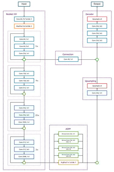
Figure A1.
Diagram of DeepLabv3+ with ResNet-101 as backbone [38]. This network architecture is the final deep convolutional neural network used to train all models to detect the necessity and the urgency of thinnings. Green circles: concatenations.
References
- Daume, S.; Robertson, D. A heuristic approach to modelling thinnings. Silva Fenn. 2000, 34, 237–249. [Google Scholar] [CrossRef]
- Mitchell, S.J. Stem growth responses in Douglas-fir and sitka spruce following thinning: Implications for assessing wind-firmness. For. Ecol. Manag. 2000, 135, 105–114. [Google Scholar] [CrossRef]
- Strütt, M. Betriebswirtschaftliche Modelluntersuchungen zu Z-Baum orientierten Produktionsstrategien in der Fichtenwirtschaft. Mitteilungen Der Forstl. Vers.- Und Forschungsanstalt Baden-WüRttemberg 1991, 156, 221. [Google Scholar]
- Spellmann, H.; Schmidt, M. Massen-, Sorten-und Wertertrag der Fichte in Abhangigkeit von der Bestandesbehandlung. Forst Und Holz 2003, 58, 412–419. [Google Scholar]
- Hynynen, J.; Ahtikoski, A.; Siitonen, J.; Sievänen, R.; Liski, J. Applying the MOTTI simulator to analyse the effects of alternative management schedules on timber and non-timber production. For. Ecol. Manag. 2005, 207, 5–18. [Google Scholar] [CrossRef]
- Hein, S.; Herbstritt, S.; Kohnle, U. Auswirkung der Z-Baum-Auslesedurchforstung auf Wachstum, Sortenertrag und Wertleistung im Europäischen Fichten-Stammzahlversuch (Picea abies [L.] Karst.) in Südwestdeutschland. Allg. Forst- Und Jagdztg. 2008, 179, 192–201. [Google Scholar]
- Juodvalkis, A.; Kairiukstis, L.; Vasiliauskas, R. Effects of thinning on growth of six tree species in north-temperate forests of Lithuania. Eur. J. For. Res. 2005, 124, 187–192. [Google Scholar] [CrossRef]
- Ghamisi, P.; Yokoya, N.; Li, J.; Liao, W.; Liu, S.; Plaza, J.; Rasti, B.; Plaza, A. Advances in Hyperspectral Image and Signal Processing: A Comprehensive Overview of the State of the Art. IEEE Geosci. Remote Sens. Mag. 2017, 5, 37–78. [Google Scholar] [CrossRef]
- Ma, L.; Liu, Y.; Zhang, X.; Ye, Y.; Yin, G.; Johnson, B.A. Deep learning in remote sensing applications: A meta-analysis and review. ISPRS J. Photogramm. Remote Sens. 2019, 152, 166–177. [Google Scholar] [CrossRef]
- Hyvönen, P.; Heinonen, J.; Haara, A. Detection of forest management operations using Bi-temporal aerial photographs. Int. Arch. Photogramm. Remote Sens. Spat. Inf. Sci.—ISPRS Arch. 2010, 38, 309–313. [Google Scholar]
- Yu, X.; Hyyppä, J.; Kaartinen, H.; Maltamo, M. Automatic detection of harvested trees and determination of forest growth using airborne laser scanning. Remote Sens. Environ. 2004, 90, 451–462. [Google Scholar] [CrossRef]
- Ballanti, L.; Blesius, L.; Hines, E.; Kruse, B. Tree species classification using hyperspectral imagery: A comparison of two classifiers. Remote Sens. 2016, 8, 445. [Google Scholar] [CrossRef]
- Fricker, G.A.; Ventura, J.D.; Wolf, J.A.; North, M.P.; Davis, F.W.; Franklin, J. A convolutional neural network classifier identifies tree species in mixed-conifer forest from hyperspectral imagery. Remote Sens. 2019, 11, 2326. [Google Scholar] [CrossRef]
- Immitzer, M.; Neuwirth, M.; Böck, S.; Brenner, H.; Vuolo, F.; Atzberger, C. Optimal input features for tree species classification in Central Europe based on multi-temporal Sentinel-2 data. Remote Sens. 2019, 11, 2599. [Google Scholar] [CrossRef]
- Axelsson, A.; Lindberg, E.; Reese, H.; Olsson, H. Tree species classification using Sentinel-2 imagery and Bayesian inference. Int. J. Appl. Earth Obs. Geoinf. 2021, 100, 102318. [Google Scholar] [CrossRef]
- Halme, E.; Pellikka, P.; Mõttus, M. Utility of hyperspectral compared to multispectral remote sensing data in estimating forest biomass and structure variables in Finnish boreal forest. Int. J. Appl. Earth Obs. Geoinf. 2019, 83, 101942. [Google Scholar] [CrossRef]
- Bohlin, J.; Bohlin, I.; Jonzén, J.; Nilsson, M. Mapping forest attributes using data from stereophotogrammetry of aerial images and field data from the national forest inventory. Silva Fenn. 2017, 51, 1–18. [Google Scholar] [CrossRef]
- Ganz, S.; Käber, Y.; Adler, P. Measuring tree height with remote sensing-a comparison of photogrammetric and LiDAR data with different field measurements. Forests 2019, 10, 694. [Google Scholar] [CrossRef]
- Hyvönen, P. Kuvioittaisten puustotunnusten ja toimen- pide-ehdotusten estimointi k-lähimmän naapurin menetel- mällä Landsat TM -satelliittikuvan, vanhan inventointitiedon ja kuviotason tukiaineiston avulla [Estimation of stand characteristics and forest management op. Metsätieteen Aikakauskirja 2002, 2, 363–379. [Google Scholar]
- Vastaranta, M.; Holopainen, M.; Yu, X.; Hyyppä, J.; Hyyppä, H.; Viitala, R. Predicting stand-thinning maturity from airborne laser scanning data. Scand. J. For. Res. 2011, 26, 187–196. [Google Scholar] [CrossRef]
- Haara, A.; Korhonen, K.T. Toimenpide-ehdotusten simulointi laskennallisesti ajantasaistetusta kuvioaineistosta. Metsätieteen Aikakauskirja 2004, 2004, 157–173. [Google Scholar] [CrossRef]
- Liu, C.C.; Zhang, Y.C.; Chen, P.Y.; Lai, C.C.; Chen, Y.H.; Cheng, J.H.; Ko, M.H. Clouds Classification from Sentinel-2 Imagery with Deep Residual Learning and Semantic Image Segmentation. Remote Sens. 2019, 11, 119. [Google Scholar] [CrossRef]
- Long, J.; Shelhamer, E.; Darrell, T. Fully convolutional networks for semantic segmentation. In Proceedings of the IEEE Computer Society Conference on Computer Vision and Pattern Recognition, Boston, MA, USA, 7–12 June 2015; pp. 3431–3440. [Google Scholar] [CrossRef]
- Volpi, M.; Tuia, D. Deep multi-task learning for a geographically-regularized semantic segmentation of aerial images. ISPRS J. Photogramm. Remote Sens. 2018, 144, 48–60. [Google Scholar] [CrossRef]
- Yue, K.; Yang, L.; Li, R.; Hu, W.; Zhang, F.; Li, W. TreeUNet: Adaptive Tree convolutional neural networks for subdecimeter aerial image segmentation. ISPRS J. Photogramm. Remote Sens. 2019, 156, 1–13. [Google Scholar] [CrossRef]
- Diakogiannis, F.I.; Waldner, F.; Caccetta, P.; Wu, C. ResUNet-a: A deep learning framework for semantic segmentation of remotely sensed data. ISPRS J. Photogramm. Remote Sens. 2020, 162, 94–114. [Google Scholar] [CrossRef]
- Ronneberger, O.; Fischer, P.; Brox, T. U-net: Convolutional networks for biomedical image segmentation. In Proceedings of the Lecture Notes in Computer Science (Including Subseries Lecture Notes in Artificial Intelligence and Lecture Notes in Bioinformatics); Springer: Berlin/Heidelberg, Germany, 2015; Volume 9351, pp. 234–241. [Google Scholar] [CrossRef]
- Hordiiuk, D.; Oliinyk, I.; Hnatushenko, V.; Maksymov, K. Semantic segmentation for ships detection from satellite imagery. In Proceedings of the 2019 IEEE 39th International Conference on Electronics and Nanotechnology (ELNANO), Kyiv, Ukraine, 16–18 April 2019; pp. 454–457. [Google Scholar]
- Chen, Z.; Wang, C.; Li, J.; Fan, W.; Du, J.; Zhong, B. Adaboost-like End-to-End multiple lightweight U-nets for road extraction from optical remote sensing images. Int. J. Appl. Earth Obs. Geoinf. 2021, 100, 102341. [Google Scholar] [CrossRef]
- Stoian, A.; Poulain, V.; Inglada, J.; Poughon, V.; Derksen, D. Land cover maps production with high resolution satellite image time series and convolutional neural networks: Adaptations and limits for operational systems. Remote Sens. 2019, 11, 1986. [Google Scholar] [CrossRef]
- He, K.; Sun, J. Convolutional neural networks at constrained time cost. In Proceedings of the IEEE Computer Society Conference on Computer Vision and Pattern Recognition, Boston, MA, USA, 7–12 June 2015; pp. 5353–5360. [Google Scholar] [CrossRef]
- He, K.; Zhang, X.; Ren, S.; Sun, J. Deep residual learning for image recognition. In Proceedings of the IEEE Computer Society Conference on Computer Vision and Pattern Recognition, Las Vegas, NV, USA, 27–30 June 2016; pp. 770–778. [Google Scholar] [CrossRef]
- Huang, G.; Liu, Z.; Van Der Maaten, L.; Weinberger, K.Q. Densely connected convolutional networks. In Proceedings of the 30th IEEE Conference on Computer Vision and Pattern Recognition, CVPR 2017, Honolulu, HI, USA, 21–26 July 2017; pp. 2261–2269. [Google Scholar] [CrossRef]
- Jegou, S.; Drozdzal, M.; Vazquez, D.; Romero, A.; Bengio, Y. The One Hundred Layers Tiramisu: Fully Convolutional DenseNets for Semantic Segmentation. In Proceedings of the IEEE Computer Society Conference on Computer Vision and Pattern Recognition Workshops, Honolulu, HI, USA, 21–26 July 2017; pp. 1175–1183. [Google Scholar] [CrossRef]
- Chen, L.C.; Papandreou, G.; Kokkinos, I.; Murphy, K.; Yuille, A.L. Semantic image segmentation with deep convolutional nets and fully connected crfs. arXiv 2014, arXiv:1412.7062. [Google Scholar]
- He, K.; Zhang, X.; Ren, S.; Sun, J. Spatial Pyramid Pooling in Deep Convolutional Networks for Visual Recognition. IEEE Trans. Pattern Anal. Mach. Intell. 2015, 37, 1904–1916. [Google Scholar] [CrossRef]
- Chen, L.C.; Papandreou, G.; Kokkinos, I.; Murphy, K.; Yuille, A.L. DeepLab: Semantic Image Segmentation with Deep Convolutional Nets, Atrous Convolution, and Fully Connected CRFs. IEEE Trans. Pattern Anal. Mach. Intell. 2018, 40, 834–848. [Google Scholar] [CrossRef]
- Chen, L.C.; Zhu, Y.; Papandreou, G.; Schroff, F.; Adam, H. Encoder-decoder with atrous separable convolution for semantic image segmentation. arXiv 2018, arXiv:1802.02611. [Google Scholar]
- Liu, M.; Fu, B.; Xie, S.; He, H.; Lan, F.; Li, Y.; Lou, P.; Fan, D. Comparison of multi-source satellite images for classifying marsh vegetation using DeepLabV3 Plus deep learning algorithm. Ecol. Indic. 2021, 125, 107562. [Google Scholar] [CrossRef]
- Holgén, P.; Söderberg, U.; Hånell, B. Diameter increment in Picea abies shelterwood stands in northern Sweden. Scand. J. For. Res. 2003, 18, 163–167. [Google Scholar] [CrossRef]
- Stirling, G.; Gardiner, B.; Macdonald, E.; Mochan, S.; Connolly, T. Stem Straightness in Sitka Spruce in South Scotland; Technical Report; Forest Research, UK Forestry Commission: Roslin, UK, 2000.
- Macdonald, E.; Gardiner, B.; Mason, W. The effects of transformation of even-aged stands to continuous cover forestry on conifer log quality and wood properties in the UK. Forestry 2010, 83, 1–16. [Google Scholar] [CrossRef]
- Persson, P. Windthrow in forests-its causes and the effect of forestry measures [Sweden, Scots pine, Norway spruce]. In Rapporter och Uppsatser-Skogshoegskolan; Institutionen foer Skogsproduktion: Umeå, Sweden, 1975. [Google Scholar]
- MacKenzie, R.F. Silviculture and management in relation to risk of windthrow in Northern Ireland. Ir. For. 1976, 33, 29–38. [Google Scholar]
- Slodicak, M.; Novak, J.; Skovsgaard, J.P. Wood production, litter fall and humus accumulation in a Czech thinning experiment in Norway spruce (Picea abies (L.) Karst.). For. Ecol. Manag. 2005, 209, 157–166. [Google Scholar] [CrossRef]
- Pollanschutz, J. Erfahrung aus der Schneebruchkatastrophe 1979. Allegem. Forstztg. 1980, 91, 123–125. [Google Scholar]
- Valinger, E.; Fridman, J. Models to assess the risk of snow and wind damage in pine, spruce, and birch forests in Sweden. Environ. Manag. 1999, 24, 209–217. [Google Scholar] [CrossRef]
- Valinger, E.; Lövenius, M.O.; Johansson, U.; Fridman, J.; Claeson, S.; Gustafsson, Å. Analys av Riskfaktorer efter Stormen Gudrun; Technical Report; Swedish Forest Agency–Skogsstyrelsen, Swedish University of Agricultural Sciences: Uppsala, Sweden, 2006. [Google Scholar]
- Schütz, J.P.; Götz, M.; Schmid, W.; Mandallaz, D. Vulnerability of spruce (Picea abies) and beech (Fagus sylvatica) forest stands to storms and consequences for silviculture. Eur. J. For. Res. 2006, 125, 291–302. [Google Scholar] [CrossRef]
- Cameron, A.D. Importance of early selective thinning in the development of long-term stand stability and improved log quality: A review. Forestry 2002, 75, 25–35. [Google Scholar] [CrossRef]
- Abetz, P. Biologische Produktionsmodelle als Entscheidungshilfen im Waldbau. Forstarchiv 1970, 41, 5–9. [Google Scholar]
- Avery, T.E. Forester’s Guide to Aerial Photo Interpretation; Number 308 in Agriculture Handbook; US Department of Agriculture, Forest Service: Washington, DC, USA, 1969.
- Kangas, A.; Astrup, R.; Breidenbach, J.; Fridman, J.; Gobakken, T.; Korhonen, K.T.; Maltamo, M.; Nilsson, M.; Nord-Larsen, T.; Næsset, E.; et al. Remote sensing and forest inventories in Nordic countries–roadmap for the future. Scand. J. For. Res. 2018, 33, 397–412. [Google Scholar] [CrossRef]
- Holopainen, M.; Vastaranta, M.; Hyyppä, J. Outlook for the next generation’s precision forestry in Finland. Forests 2014, 5, 1682–1694. [Google Scholar] [CrossRef]
- Magnussen, S.; Nord-Larsen, T.; Riis-Nielsen, T. Lidar supported estimators of wood volume and aboveground biomass from the Danish national forest inventory (2012–2016). Remote Sens. Environ. 2018, 211, 146–153. [Google Scholar] [CrossRef]
- Olesk, A.; Voormansik, K.; Põhjala, M.; Noorma, M. Forest change detection from Sentinel-1 and ALOS-2 satellite images. In Proceedings of the 2015 IEEE 5th Asia-Pacific Conference on Synthetic Aperture Radar, APSAR 2015, Marina Bay Sands, Singapore, 1–4 September 2015; pp. 522–527. [Google Scholar] [CrossRef]
- basemap. Orthofoto TileCache of Austria; geoland.at: 2021. Available online: https://geoland.at/ (accessed on 19 August 2023).
- Gruber, M.; Ponticelli, M.; Ladstädter, R.; Wiechert, A. Ultracam Eagle, Details and Insight. Int. Arch. Photogramm. Remote Sens. Spat. Inf. Sci. 2012, 39, 15–19. [Google Scholar] [CrossRef]
- Horn, B.K. Hill Shading and the Reflectance Map. Proc. IEEE 1981, 69, 14–47. [Google Scholar] [CrossRef]
- GDAL/OGR Contributors. GDAL/OGR Geospatial Data Abstraction Software Library; Open Source Geospatial Foundation: Beaverton, OR, USA, 2022. [Google Scholar] [CrossRef]
- Wikipedia. Salvage Logging. 2023. Available online: https://en.wikipedia.org/wiki/Salvage_logging (accessed on 19 August 2023).
- Satlawa, P. Detecting the Necessity of Thinnings with Deep Learning. Master’s Thesis, School of Informatics, University of Edinburgh, Edinburgh, UK, 2021. [Google Scholar]
- Snoek, J.; Larochelle, H.; Adams, R.P. Practical Bayesian optimization of machine learning algorithms. Adv. Neural Inf. Process. Syst. 2012, 25, 2960–2968. [Google Scholar]
- He, K.; Zhang, X.; Ren, S.; Sun, J. Delving deep into rectifiers: Surpassing human-level performance on imagenet classification. In Proceedings of the IEEE International Conference on Computer Vision, Santiago, Chile, 11–18 December 2015; pp. 1026–1034. [Google Scholar] [CrossRef]
- Kingma, D.P.; Ba, J.L. Adam: A method for stochastic optimization. In Proceedings of the 3rd International Conference on Learning Representations, ICLR 2015–Conference Track Proceedings, San Diego, CA, USA, 7–9 May 2015; pp. 1–13. [Google Scholar]
- Jadon, S. A survey of loss functions for semantic segmentation. In Proceedings of the 2020 IEEE Conference on Computational Intelligence in Bioinformatics and Computational Biology, CIBCB 2020, Virtual Conference, 27–29 October 2020. [Google Scholar] [CrossRef]
Disclaimer/Publisher’s Note: The statements, opinions and data contained in all publications are solely those of the individual author(s) and contributor(s) and not of MDPI and/or the editor(s). MDPI and/or the editor(s) disclaim responsibility for any injury to people or property resulting from any ideas, methods, instructions or products referred to in the content. |
© 2023 by the authors. Licensee MDPI, Basel, Switzerland. This article is an open access article distributed under the terms and conditions of the Creative Commons Attribution (CC BY) license (https://creativecommons.org/licenses/by/4.0/).