Optimal Integration of Flexible Alternating Current Transmission Systems in Electrical Distribution Grids Using a Mixed-Integer Convex Model

Abstract

This research addresses the efficient integration and sizing of flexible alternating current transmission systems (FACTS) in electrical distribution networks via a convex optimization approach. The exact mixed-integer nonlinear programming (MINLP) model associated with FACTS siting and sizing aims for the minimization of the expected annual operating costs of the network (i.e., energy losses and FACTS purchasing costs). The constraints of this problem include power equilibrium equalities, voltage regulation bounds, and device capacities, among others. Due to the power equilibrium constraints per node and period, the MINLP model is a non-convex optimization problem. To transform the exact MINLP model into a mixed-integer convex one, the approximation of the product between two variables in the complex domain is relaxed through its hyperbolic equivalent, which generates a set of convex cones. The main advantage of the proposed mixed-integer convex model is that it ensures the global optimum of the problem, even when considering objective multiplexes. Numerical simulations in the IEEE 33-, 69-, and 85-bus grids demonstrate the effectiveness and robustness of FACTS integration via the proposed convex approach in comparison with the exact solution of the MINLP model in the GAMS software as well as with combinatorial optimization algorithms (i.e., the black widow optimizer and the vortex search algorithm). All simulations were carried out in MATLAB with Yalmip optimization and the Gurobi and Mosek solvers. The simulation results show that, for a fixed operation of the FACTS devices (i.e., a VAR compensator) during the day, the annual operating costs are reduced by 12.63%, 13.97%, and 26.53% for the IEEE 33-, 69-, and 85-bus test systems, respectively, while for the operation variable, the reductions are by 14.24%, 15.79%, and 30.31%, respectively.

1. Introduction

1.1. General Context

Electrical distribution networks in medium- and low-voltage applications provide electricity to all end-users while observing quality, security, reliability, and efficiency criteria [1,2]. These grids are typically operated at voltage levels lower or equal to 25 kV, mostly using alternating current (AC) technologies. Most of them are built with a tree structure (i.e., radial configuration) that helps to reduce investment costs and the complexity of coordinating protective devices [3,4]. However, these radial configurations typically increase energy losses when compared to meshed topologies [5], and they deteriorate the voltage profiles (low voltage regulation) for end-users located far from the central substation nodes [6]. Distribution companies typically use shunt compensation methodologies or grid topology modifications to address these technical challenges. In the case of shunt compensation, active and reactive power injection devices are commonly used (dispersed generation [7], batteries [8], capacitors [9], or flexible AC transmission systems [10,11], i.e., FACTS). In contrast, in the case of topology modifications, phase balancing or grid reconfiguration are common strategies for distribution companies. In the case of power loss reduction or voltage profile improvement, shunt reactive power compensation has demonstrated an adequate balance between saving operating costs regarding energy losses compared to the investment costs associated with compensation systems [9].

On the other hand, given the transition of electrical distribution networks from passive to active operation schemes [12], the use of fixed compensation strategies [13], such as capacitor banks or grid topology variations, results in low economic savings in comparison with dynamic compensation strategies using FACTS [10].

The use of FACTS compensation devices in electrical distribution networks has shown positive effects on the technical characteristics of electrical grids, especially in the case of energy losses minimization, with improvements of about 12.63% and 13.97% in the conventional IEEE 33- and 69-bus systems [10]. In addition, for distribution networks in the Colombian context, energy losses can oscillate between 14.5% and 21.8% of the total energy input [10]. This implies that the development of compensation technologies for reducing these losses is essential for distribution companies. In this regard, one of the advantages of reactive power compensation systems is that they are reliable [14] and economical [15], in addition to the fact that they have long useful lives [16].

1.2. Motivation

The efficient integration (nodal location and nominal size) and operation (on an hourly basis) of FACTS in electrical distribution networks pose fundamental challenges regarding the nature of this optimization problem as it belongs to the family of mixed-integer nonlinear programming (MINLP) [17]. Given the complexity of the exact model, this research aims to propose an efficient solution methodology to locate and size FACTS in medium-voltage distribution networks by reformulating the MINLP model as a mixed-integer convex approximation [18]. The main advantage of convex optimization is that it allows representing optimization problems in engineering and science while ensuring a global optimal solution [19]. This research aims to provide the literature and the industry with an efficient and reliable solution methodology to address the studied problem, with superior performance compared to MINLP solvers in commercial software or metaheuristic algorithms [18].

It is important to mention that studying the problem regarding the optimal location and sizing of FACTS in electrical distribution networks is necessary since:

• Dynamic reactive power compensation is an area of continuous development due to the quality impositions of regulatory offices on distribution companies, which aim to make their medium-voltage distribution grids efficient, reliable, and secure [20]. To this effect, effective optimization algorithms must be proposed;
• Most existing solution methodologies focus on metaheuristic optimization algorithms to deal with the exact MINLP formulation via decoupling-based approaches that work under a master–slave optimization strategy [21]. However, even though these master–slave approaches are efficient and easily implemented in multiple programming languages, they do not allow ensuring a global optimum, given the random nature of heuristic-based optimizers [22]. Therefore, this research takes advantage of mixed-integer convex programming to propose an efficient solution methodology to locate and size FACTS in electrical networks while allowing us to find the global optimum [23].

1.3. Literature Review

The problem regarding the optimal placement and sizing of FACTS in medium- and low-voltage distribution networks has been widely explored in the specialized literature. This section summarizes the most recent approaches in this research area.

The authors of [11] applied the hunter–prey algorithm to determine the optimal location and sizing of photovoltaic-SVC systems in electrical distribution networks, with the aim to minimize grid power losses and improve system voltage profiles. The main characteristic of a photovoltaic-SVC system is that it can use the converter interfacing with the photovoltaic (PV) system to add reactive power injection capabilities via control design [24]. The numerical results presented in [11] for the IEEE 33- and 69-bus grids demonstrated the effectiveness of the proposed hunter–prey optimizer when compared to different combinatorial methods, such as the differential evolution algorithm, particle swarm optimization, the artificial rabbits algorithm, and the golden search optimizer.

The work by [25] presented a complete comparative analysis of multiple combinatorial optimizers in locating and sizing TCSCs and SVCs in power systems while aiming to minimize the total grid operating costs associated with energy losses. The voltage profiles were kept within an acceptable range. Numerical validations in the IEEE 30- and 57-bus systems were used to test the effectiveness of the whale optimization algorithm in comparison with multiple combinatorial optimizers.

In [10], the black widow optimization algorithm was proposed as a solution method to locate and size FACTS in medium-voltage distribution networks. The exact MINLP model was solved using a leader–follower optimization strategy, combining a discrete-continuous codification in the leader stage with a black widow optimizer using the successive approximations of power flow in the follower stage. Numerical results in the IEEE 33-, 69-, and 85-bus grids demonstrated the effectiveness of the leader-follower solution compared to that of the vortex search algorithm reported in [26]. All this, while considering the minimization of investment and operating costs as objective functions.

The authors of [27] presented a complete review of the optimal location and sizing of SVCs in electrical distribution networks while considering the technical and economic aspects of the objective function. Five approaches regarding solution technologies were reviewed, which include artificial neural network techniques, analytical methods, combinatorial methods, and sensitivity approaches. This review demonstrated that SVCs are suitable FACTS for improving grid voltage profiles, enhancing stability indices, and reducing grid power losses with reasonable investments by utility companies. Thus, SVCs are a feasible economic solution for compensating reactive power in these networks.

The study by [28] presented a solution methodology to locate and size SVCs in distribution networks while considering load variations via a nodal sensitivity approach. Efficient numerical validation in practical distribution networks composed of 38 nodes demonstrated important improvements with regard to different objective functions, including energy losses cost reduction, voltage profile improvements, and stability margin enhancement.

Other solution methods for locating and sizing FACTS in distribution networks are the tabu search algorithm [29,30], the fractional levy flight bat algorithm [31], the particle swarm optimizer [32], the krill herd algorithm [33], and the barnacles mating optimization [34], among others.

All of the works reviewed above yielded good solutions. However, none of them can guarantee the optimal solution to the problem, and some require tuning parameters, which indicates that, if the test systems are changed, they may not reach reasonable solutions and thus require adjustments.

1.4. Contribution and Scope

In light of the above, it is worth noting that, in order to analyze it, the problem under study is standardized via the application of leader-follower optimization techniques (combinatorial methods to decide on the location of the FACTS and optimal power flows to determine their sizes). This provides a research opportunity in the area of convex optimization. In this sense, the main contributions of this research are presented below:

• A reformulation of the exact MINLP model regarding the efficient location and sizing of FACTS in distribution networks via a mixed-integer second-order cone programming equivalent. This reformulation can guarantee the global optimum of the problem. Thus, it finds the best solution to the optimization problem according to its fitness function.
• The evaluation of multiple operation scenarios where the FACTS can be operated as fixed or variable compensators. These scenarios demonstrated that variable compensation is the best option to reduce the annual grid operating costs.

Note that, within the scope of this research, the FACTS devices analyzed correspond to the shunt reactive power compensation elements studied by [10]. These devices are the unified power flow controller (UPFC), the thyristor-controlled shunt compensator (TCSC), and the static var compensator (SVC). The investment costs of installing these devices are modeled as a cubic function based on the recommendations of [35]. In addition, the active and reactive power curves are inputs provided by the distribution company at the terminals of the substation bus, representing the electrical network’s daily behavior. Here, these curves are assumed as constants without noise (uncertainties). However, future research will be required to include the stochastic behavior of these curves in distribution systems analysis, operation, and control.

1.5. Document Structure

The remainder of this document is structured as follows. Section 2 presents the general MINLP model regarding the optimal location and sizing of FACTS in electrical distribution networks, with the aim to minimize the annual grid operating costs while including the investment costs of FACTS. Section 3 shows the second-order cone approximation based on the hyperbolic relation of the product between two variables, which generates a linear objective function with a set of linear and conic constraints that belongs to the family of convex optimization problems. Section 4 outlines the main characteristics of the IEEE test feeders under analysis. These systems are composed of 33, 69, and 85 nodes with medium-voltage profiles and typical radial structures. Section 5 describes the main numerical simulations carried out, a comparative study with literature reports and exact MINLP solvers, and a comparative analysis between all the studied FACTS devices, considering fixed and variable reactive power injections. Section 6 describes this article’s main concluding remarks and possible future improvements.

2. Optimization Model

The problem regarding the optimal integration of FACTS devices in electrical distribution grids aims to minimize the annual costs related to energy losses and the investments made in FACTS installation. This problem generates an optimization model with the structure of a mixed-integer nonlinear programming (MINLP) model. This is because the optimization model contains binary/integer variables related to the location of the FACTS devices. At the same time, the model includes the continuous variables associated with power flows, nodal voltages, and the size of the FACTS devices. 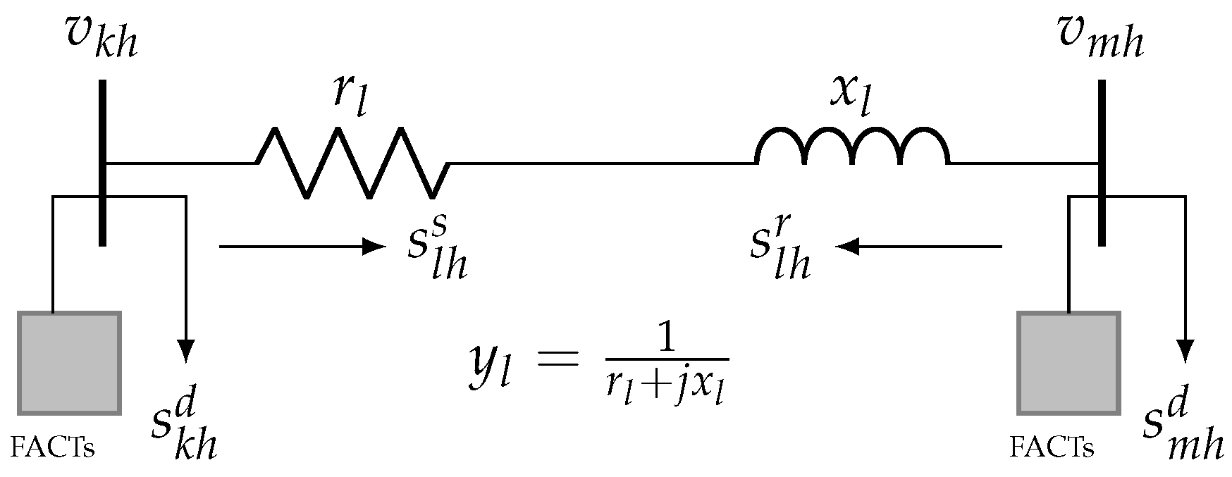Figure 1 illustrates an example of a branch in an electrical network with FACTS devices installed.

In this paper, the following notation is used. The sets $\mathcal{H}$, $\mathcal{B}$, and $\mathcal{N}$ encompass all the analysis periods, network branches, and network nodes, respectively. $\mathcal{R}$ and $\mathcal{C}$ denote the sets of real and complex numbers, respectively. The subscripts k or m denote the nodes of the test system, the subscript l represents any branch connected between nodes k and m, and the subscript h represents a specific period under analysis. The superscripts s and r denote the sending and receiving power flows of the distribution line connected between nodes k and m, while the superscripts g and d represent variables related to generation and demand, respectively. The variable v denotes the nodal voltage, and s corresponds to apparent power in a node or distribution line. The operator $∥·∥$ denotes the Euclidean norm, while the operators $real\left(·\right)$ and $imag\left(·\right)$ correspond to the real and imaginary part of the complex number, respectively. Finally, ${(·)}^{\ast }$ represents the conjugate of the complex number.

2.1. Objective Function

The main aim of this study is to incorporate FACTS devices into electrical distribution networks while aiming to minimize the annual equivalent operating costs represented by f. These costs consider the reduction of energy losses and the installation expenses associated with FACTS. To this effect, the following objective function is used:

$$\begin{array}{c}\hfill \begin{array}{cc}\hfill min& f=f_1+f_2,\hfill \\ \hfill f_1& =CT\sum _{h\in \mathcal{H}}\sum _{l\in \mathcal{B}}\left(p_{lh}^s+p_{lh}^r\right)\mathsf{\Delta }h,\hfill \\ \hfill f_2& =T\left(\frac{k_1}{k_2}\right)\sum _{k\in \mathcal{N}}{q}_k^{FACT}\left({\omega }_1{\left(q_k^{FACT}\right)}^2+{\omega }_2{q}_k^{FACT}+{\omega }_3\right),\hfill \end{array}\end{array}$$

(1)

where $f_1$ is related to the annual energy loss costs; $f_2$ is associated with the FACTS investment costs; C and T are the average costs of energy losses and the number of days in a year, respectively; $p_{lh}^s$ and $p_{lh}^r$ represent the sending and receiving active power flows of a distribution line, respectively; $\mathsf{\Delta }h$ represents the time interval analyzed on a daily basis (0.5 h); $q_k^{FACT}$ is the nominal size of the FACTS; ${\omega }_1$, ${\omega }_2$, and ${\omega }_3$ represent the polynomial coefficients of the objective function $f_2$; and $k_1>0$ and $k_2>0$ are constants denoting the annual investment costs for a planning horizon of ten years [18].

2.2. Set of Constraints

The constraints related to the optimal integration of FACTS in electrical distribution grids comprise several aspects, such as node power balance constraints for both active and reactive power, the limits regarding the maximum and minimum power flowing through the distribution lines, voltage regulation bounds, requirements regarding the number of FACTS devices to be installed, and their capacity for injecting or observing reactive power, among others.

2.2.1. Power Balance Equation

The nodal power balance equations for node k with regard to active and reactive power require calculating the sums of power generated or demanded, i.e., for active and reactive power. These sums are then equalized to the flow of injection power, be it active or reactive. The equations can be expressed as follows:

$$\begin{array}{cc}\hfill p_{kh}^g-p_{kh}^d=\sum _{l\in L}\left(A_{kl}^{+}{p}_{lh}^s+A_{kl}^{-}{p}_{lh}^r\right),& \forall k\in \mathcal{N},\forall h\in \mathcal{H},\hfill \end{array}$$

(2)

$$\begin{array}{cc}\hfill q_{kh}^g-q_{kh}^d+q_{kh}^{FACT}=\sum _{l\in L}\left(A_{kl}^{+}{q}_{lh}^s+A_{kl}^{-}{q}_{lh}^r\right),& \forall k\in \mathcal{N},\forall h\in \mathcal{H}\hfill \end{array}$$

(3)

where $p_{kh}^g$ and $p_{kh}^d$ are the active power generated and demanded; $q_{kh}^g$ and $q_{kh}^d$ are the reactive power generated and demanded; $p_{lh}^s$ and $q_{lh}^s$ are the sending active and reactive power flows of the distribution line l; $p_{lh}^r$ and $q_{lh}^r$ are the receiving active and reactive power flows of the distribution line l; $q_{kh}^{FACT}$ is the reactive power injected by the FACTS at node k and time h; and $A^{+}$ and $A^{-}$ are the positive and negative values of the node-to-branch incidence matrix A, i.e., $A=A^{+}+A^{-}$.

2.2.2. Power Flow Equation

The active and reactive power flows transmitted through a specific distribution line, along with their corresponding maximum capacities, can be represented as follows:

$$\begin{array}{c}\hfill p_{lh}^s=real\left(v_{kh}{y}_l^{\ast }{\left(v_{kh}-v_{mh}\right)}^{\ast }\right),\forall l\in \mathcal{B},\forall h\in \mathcal{H},\end{array}$$

(4)

$$\begin{array}{c}\hfill p_{lh}^r=real\left(v_{mh}{y}_l^{\ast }{\left(v_{mh}-v_{kh}\right)}^{\ast }\right),\forall l\in \mathcal{B},\forall h\in \mathcal{H},\end{array}$$

(5)

$$\begin{array}{c}\hfill q_{lh}^s=imag\left(v_{kh}{y}_l^{\ast }{\left(v_{kh}-v_{mh}\right)}^{\ast }\right),\forall l\in \mathcal{B},\forall h\in \mathcal{H},\end{array}$$

(6)

$$\begin{array}{c}\hfill q_{lh}^r=imag\left(v_{mh}{y}_l^{\ast }{\left(v_{mh}-v_{kh}\right)}^{\ast }\right),\forall l\in \mathcal{B},\forall h\in \mathcal{H},\end{array}$$

(7)

$$\begin{array}{c}\hfill \hspace{1em}\hspace{1em}\hspace{1em}\hspace{1em}\hspace{1em} ∥p_{lh}^s+j{q}_{lh}^s∥\le s_l^{max},\forall l\in \mathcal{B},\forall h\in \mathcal{H}\end{array}$$

(8)

$$\begin{array}{c}\hfill \hspace{1em}\hspace{1em}\hspace{1em}\hspace{1em}\hspace{1em} ∥p_{lh}^r+j{q}_{lh}^r∥\le s_l^{max},\forall l\in \mathcal{B},\forall h\in \mathcal{H}\end{array}$$

(9)

where $v_{kh}$ and $v_{mh}$ are the complex voltages, $y_l$ is the admittance of branch l, and $s_l^{max}$ is the maximum apparent power flowing through the line.

2.2.3. Operating Regulations

All node voltage values in an electrical network must meet the limits set by regulatory policies, which are intended for an adequate network operation. These limits are

$$\begin{array}{cc}\hfill v_{0h}=v^{\mathrm{nom}}{e}^{j0},& \forall h\in \mathcal{H},\hspace{1em}\hspace{1em}\hspace{1em}\hspace{1em}\hspace{1em}\hfill \end{array}$$

(10)

$$\begin{array}{cc}\hfill ∥v_{ht}∥\ge v^{min},& \forall k\in \mathcal{N},\forall h\in \mathcal{H},\hfill \end{array}$$

(11)

$$\begin{array}{cc}\hfill ∥v_{ht}∥\le v^{max},& \forall k\in \mathcal{N},\forall h\in \mathcal{H},\hfill \end{array}$$

(12)

where $v_{0h}$ represents the nominal voltage at the slack node (substation) at time h; $v^{\mathrm{nom}}$ is its nominal value, which usually has a per-unit value equal to 1.0; and $v^{min}$ and $v^{max}$ denote the minimum and maximum voltage values allowed in the electrical network.

2.2.4. Integration of FACTS

The optimal integration of the FACTS is divided into two parts, which include their proper location in the electrical grid as well as their size. The following constraints are defined to address these challenges:

$$\begin{array}{cc}\hfill 0\le q_k^{FACT}\le z_k{q}_{max}^{\mathrm{FACT}},& \forall k\in \mathcal{N},\hfill \end{array}$$

(13)

$$\begin{array}{cc}\hfill -q_k^{FACT}\le q_{kh}^{FACT}\le q_k^{FACT},& \forall k\in \mathcal{N},\forall h\in \mathcal{H}\hfill \end{array}$$

(14)

$$\begin{array}{c}\hfill \sum _{k\in \mathcal{N}}{z}_k\le \eta ,\end{array}$$

(15)

$$\begin{array}{cc}\hfill z_k\in \left\{0,1\right\},& \forall k\in \mathcal{N},\hfill \end{array}$$

(16)

where $q_k^{FACT}$ is the variable used to define the size of the FACTS to be installed, and $q_{max}^{\mathrm{FACT}}$ is its maximum capacity. This study’s capacity goes from 0 Mvar to 2 Mvar at the distribution level, a value usually employed for electrical networks [18]. z is a vector of the binary variable that denotes a FACTS location at node k, i.e., if $z=1$ in position k, this indicates that a device will be located there (otherwise, $z=0$). Finally, $\eta$ is the maximum number of FACTS to be installed.

2.3. Interpretation of the Mathematical Model

The mixed-integer nonlinear optimization model described in (1)–(16) aims to optimize FACTS integration in electrical distribution grids. This model incorporates both binary and continuous variables. The placement of these devices is determined by the former. The latter is associated with several variables, including the active and reactive power of the generators, power demands, the power flowing through the transmission lines, complex nodal voltages, and the size of the FACTS.

The following can be noted regarding this mixed-integer nonlinear optimization model. The objective function is defined by two terms. The first term, which implies an annual cost of $f_1$, represents the energy losses of the electrical distribution system. In contrast, the second term calculates the investment costs of FACTS ($f_2$). Expressions (2) and (3) represent the active and reactive power balance, respectively, for each node and time period under analysis. Equations (4) and (5) represent the active power flow that is transmitted through each branch of the transmission lines at each studied time interval. Equations (6) and (7) represent the reactive power flowing through the same transmission lines. Inequalities (8) and (9) limit the maximum apparent power that can flow through each branch of the transmission lines in any given period. Equation (10) sets the voltage at the substation, while inequalities (11) and (12) constrain the nodal voltages to their respective minimum and maximum values at each time step. Inequality (13) restricts the maximum value that the FACTS may reach. Inequality (14) sets the limit for the maximum reactive power that the FACTS may deliver or absorb at each node. Finally, inequality (15) determines the maximum number of FACTS that can be installed.

3. Convex Reformulation

The optimization model described in Equations (1)–(16) is a mixed-integer nonlinear one, which is challenging to solve and falls into the category of problems with high computational complexity. Therefore, this type of problem is typically solved using a metaheuristic algorithm [18,36]. However, metaheuristic algorithms cannot ensure the global optimum of the problem. Additionally, many of these algorithms require parameter tuning, which indicates that their performance is not always consistent. Another potential solution to this problem is introducing some relaxations that can transform the mixed-integer nonlinear model into a mixed-convex one, thus being able to guarantee the global optimum of the problem. Nevertheless, this also requires parameter tuning.

3.1. Approximation of the Objective Function $z_2$ to Linear Function

The objective function $f_2$ presented in (1) has a cubic form, which makes it a non-convex function. Therefore, it is impossible to guarantee the global optimum of the problem. However, this objective function can only work with a linear coefficient ${\omega }_3$ for a range of FACTS with values lower than or equal to 2 Mvar [18]. The objective function $z_2$ is expressed as follows:

$$\begin{array}{c}\hfill z_2=T\left(\frac{k_1}{k_2}\right){\omega }_3\sum _{k\in \mathcal{N}}{q}_k^{FACT}.\end{array}$$

(17)

3.2. Convex Representation of the Active and Reactive Power Flow Equations

The products of the voltages presented in the active and reactive power flow equations, as described in (4)–(7), are equality constraints. Hence, they are non-convex constraints. However, it is possible to convert these constraints into convex ones by defining two auxiliary variables [37], as follows:

$$\begin{array}{c}\hfill u_{kh}=v_{kh}{v}_{kh}^{\ast }={∥v_{kh}∥}^2,\end{array}$$

(18)

$$\begin{array}{c}\hfill \hspace{1em}\hspace{1em}\hspace{1em}\hspace{1em}{w}_{lh}=v_{kh}{v}_{mh}^{\ast }\end{array}$$

(19)

where $u_{kh}\in \mathcal{R}$ corresponds to the squared voltage at node k and time h, and $w_{lh}\in \mathcal{C}$ denotes the product of the voltages in branch l at time h.

Now, the auxiliary variables $u_{kh}$ and $w_{lh}$ can be substituted into the active and reactive power flow Equations (4)–(7) in order to obtain:

$$\begin{array}{cc}\hfill p_{lh}^s& =real\left(\left(u_{kh}-w_{lh}\right)y_l^{\ast }\right),\hfill \end{array}$$

(20)

$$\begin{array}{cc}\hfill p_{lh}^r& =real\left(\left(u_{mh}-w_{lh}^{\ast }\right)y_l^{\ast }\right),\hfill \end{array}$$

(21)

$$\begin{array}{cc}\hfill q_{lh}^s& =imag\left(\left(u_{kh}-w_{lh}\right)y_l^{\ast }\right),\hfill \end{array}$$

(22)

$$\begin{array}{cc}\hfill q_{lh}^r& =imag\left(\left(u_{mh}-w_{lh}^{\ast }\right)y_l^{\ast }\right).\hfill \end{array}$$

(23)

The equations for the active and reactive power flows, as presented in (20)–(23), depend on the auxiliary variables in (18) and (19). These equations are non-convex, so it is necessary to relax them via a hyperbolic shape, as shown below:

$$\begin{array}{c}\hfill \begin{array}{cc}\hfill w_{lh}& =v_{kh}{v}_{mh}^{\ast }\hfill \\ \hfill w_{lh}{w}_{kmt}^{\ast }& =v_{kh}{v}_{mh}^{\ast }{v}_{mh}{v}_{kh}^{\ast }\hfill \\ \hfill {∥w_{lh}∥}^2& ={∥v_{kh}∥}^2{∥v_{mh}∥}^2\hfill \\ \hfill {∥w_{lh}∥}^2& =u_{kh}{u}_{mh}=\frac{1}{4}{\left(u_{kh}+u_{mh}\right)}^2-\frac{1}{4}{\left(u_{kh}-u_{mh}\right)}^2\hfill \\ \hfill {\left(u_{kh}-u_{mh}\right)}^2+{∥2w_{lh}∥}^2& ={\left(u_{kh}+u_{mh}\right)}^2\hfill \\ \hfill ∥\begin{array}{c}2w_{lh}\\ u_{kh}-u_{mh}\end{array}∥& =u_{kh}+u_{mh}\hfill \\ \hfill ∥\begin{array}{c}2w_{lh}\\ u_{kh}-u_{mh}\end{array}∥& \le u_{kh}+u_{mh}.\hfill \end{array}\end{array}$$

(24)

3.3. Proposed Mixed-Integer Convex Model

The optimization model described in (1)–(16) can be transformed into a mixed-integer convex model by applying the abovementioned relaxation. The process is as follows:

$$\begin{array}{cc}\hfill min& f=z_1+z_2,\hspace{1em}\hspace{1em}\hspace{1em}\hspace{1em}\hspace{1em}\hspace{1em}\hspace{1em}\hspace{1em}\hspace{1em}\hspace{1em}\hspace{1em}\hspace{1em}\hspace{1em}\hspace{1em}\hspace{1em}\hspace{1em}\hspace{1em}\hspace{1em}\hspace{1em}\hspace{1em}\hspace{1em}\hspace{1em} \hfill \end{array}$$

(25)

$$\begin{array}{cc}\hfill & f_1=CT\sum _{h\in \mathcal{H}}\sum _{l\in \mathcal{B}}\left(p_{lh}^s+p_{lh}^r\right)\mathsf{\Delta }h,\hspace{1em}\hspace{1em}\hspace{1em}\hspace{1em}\hspace{1em}\hspace{1em}\hspace{1em}\hspace{1em}\hspace{1em}\hspace{1em}\hspace{1em}\hspace{1em} \hspace{1em}\hfill \end{array}$$

(26)

$$\begin{array}{cc}\hfill & f_2=T\left(\frac{k_1}{k_2}\right){\omega }_3\sum _{k\in \mathcal{N}}{q}_k^{FACT},\hspace{1em}\hspace{1em}\hspace{1em}\hspace{1em}\hspace{1em}\hspace{1em}\hspace{1em}\hspace{1em}\hspace{1em}\hspace{1em}\hspace{1em}\hspace{1em}\hspace{1em} \hspace{1em}\hfill \end{array}$$

(27)

$$\begin{array}{cc}\hfill & p_{kh}^g-p_{kh}^d=\sum _{l\in L}\left(A_{kl}^{+}{p}_{lh}^s+A_{kl}^{-}{p}_{lh}^r\right),\forall k\in \mathcal{N},\forall h\in \mathcal{H},\hspace{1em}\hspace{1em}\hspace{1em}\hfill \end{array}$$

(28)

$$\begin{array}{cc}\hfill & q_{kh}^g-q_{kh}^d+q_{kh}^{FACT}=\sum _{l\in L}\left(A_{kl}^{+}{q}_{lh}^s+A_{kl}^{-}{q}_{lh}^r\right),\forall k\in \mathcal{N},\forall h\in \mathcal{H},\hfill \end{array}$$

(29)

$$\begin{array}{cc}\hfill & p_{lh}^s=real\left(\left(u_{kh}-w_{lh}\right)y_l^{\ast }\right),\forall l\in \mathcal{B},\forall h\in \mathcal{H}, \hspace{1em}\hspace{1em}\hspace{1em}\hspace{1em}\hspace{1em}\hfill \end{array}$$

(30)

$$\begin{array}{cc}\hfill & p_{lh}^r=real\left(\left(u_{mh}-w_{lh}^{\ast }\right)y_l^{\ast }\right),\forall l\in \mathcal{B},\forall h\in \mathcal{H}, \hspace{1em}\hspace{1em}\hspace{1em}\hspace{1em}\hspace{1em}\hfill \end{array}$$

(31)

$$\begin{array}{cc}\hfill & q_{lh}^s=imag\left(\left(u_{kh}-w_{lh}\right)y_l^{\ast }\right),\forall l\in \mathcal{B},\forall h\in \mathcal{H}, \hspace{1em}\hspace{1em}\hspace{1em}\hspace{1em}\hspace{1em}\hfill \end{array}$$

(32)

$$\begin{array}{cc}\hfill & q_{lh}^r=imag\left(\left(u_{mh}-w_{lh}^{\ast }\right)y_l^{\ast }\right),\forall l\in \mathcal{B},\forall h\in \mathcal{H},\hspace{1em}\hspace{1em}\hspace{1em}\hspace{1em}\hspace{1em}\hfill \end{array}$$

(33)

$$\begin{array}{cc}\hfill & ∥p_{lh}^s+j{q}_{lh}^s∥\le s_l^{max},\forall l\in \mathcal{B},\forall h\in \mathcal{H}\hspace{1em} \hspace{1em}\hspace{1em}\hspace{1em}\hspace{1em}\hspace{1em}\hspace{1em}\hspace{1em}\hfill \end{array}$$

(34)

$$\begin{array}{cc}\hfill & ∥p_{lh}^r+j{q}_{lh}^r∥\le s_l^{max},\forall l\in \mathcal{B},\forall h\in \mathcal{H} \hspace{1em}\hspace{1em}\hspace{1em}\hspace{1em}\hspace{1em}\hspace{1em}\hspace{1em}\hspace{1em}\hfill \end{array}$$

(35)

$$\begin{array}{cc}\hfill & u_{0t}={\left(v^{\mathrm{nom}}\right)}^2,\forall h\in \mathcal{H}, \hspace{1em}\hspace{1em}\hspace{1em}\hspace{1em}\hspace{1em}\hspace{1em}\hspace{1em}\hspace{1em}\hspace{1em}\hspace{1em}\hspace{1em}\hspace{1em}\hspace{1em}\hspace{1em}\hfill \end{array}$$

(36)

$$\begin{array}{cc}\hfill & ∥\begin{array}{c}2w_{lh}\\ u_{kh}-u_{mh}\end{array}∥\le u_{kh}+u_{mh},\forall k\in \mathcal{N},\forall h\in \mathcal{H}, \hspace{1em}\hspace{1em}\hspace{1em}\hspace{1em}\hspace{1em}\hfill \end{array}$$

(37)

$$\begin{array}{cc}\hfill & {\left(v^{\min }\right)}^2\le u_{kh}\le {\left(v^{\max }\right)}^2,\forall k\in \mathcal{N},\forall h\in \mathcal{H},\hspace{1em}\hfill \end{array}$$

(38)

$$\begin{array}{cc}\hfill & 0\le q_k^{FACT}\le z_k{q}_{max}^{\mathrm{FACT}},\forall k\in \mathcal{N}, \hspace{1em}\hspace{1em}\hspace{1em}\hspace{1em}\hspace{1em}\hfill \end{array}$$

(39)

$$\begin{array}{cc}\hfill & -q_k^{FACT}\le q_{kh}^{FACT}\le q_k^{FACT},\forall k\in \mathcal{N},\forall h\in \mathcal{H}\hfill \end{array}$$

(40)

$$\begin{array}{cc}\hfill & \sum _{k\in \mathcal{N}}{z}_k\le \eta , \hspace{1em}\hspace{1em}\hspace{1em}\hspace{1em}\hspace{1em} \hspace{1em}\hspace{1em}\hspace{1em}\hspace{1em}\hspace{1em}\hspace{1em}\hspace{1em}\hspace{1em}\hfill \end{array}$$

(41)

$$\begin{array}{cc}\hfill & z\in \left\{0,1\right\},\forall k\in \mathcal{N}. \hspace{1em}\hspace{1em}\hspace{1em}\hspace{1em}\hspace{1em} \hspace{1em}\hspace{1em}\hspace{1em}\hspace{1em}\hspace{1em}\hfill \end{array}$$

(42)

This mixed-integer convex model can reach the global optimum of the exact optimization model described in Equations (1)–(16). This is possible only if the hyperbolic constraints are well-defined conditions, as demonstrated in [38].

4. Test System

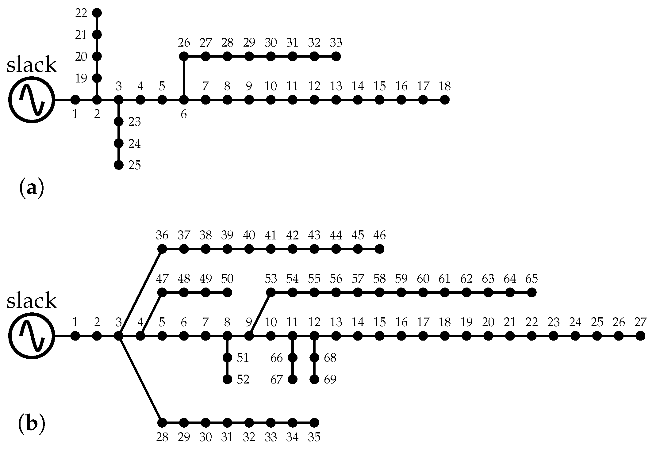
This section presents the test systems employed to validate the proposed optimization model for the optimal integration of FACTS in the IEEE 33-, 69-, and 85-bus systems. Figure 2 depicts the topologies of three test systems, whose main features are as follows:

• The IEEE 33-bus test system has 33 buses and 32 transmission lines in its radial configuration, as shown in Figure 2a. It has a substation at node 1 that works with 12.66 kV, as well as peak active and reactive demands of $3715+j2300$ kVA, respectively. These operating conditions generate active and reactive power losses of 210.9876 kW and 143.1283 kvar. The test system’s peak demand, resistance, and reactance values are listed in

  Table 1. Electrical parameters of the IEEE 33-test system.

  k	m	${\mathit{R}}_{\mathit{km}}$ ($\mathbf{\Omega }$)	${\mathit{x}}_{\mathit{km}}$ ($\mathbf{\Omega }$)	${\mathit{P}}_{\mathit{k}}$ (kW)	${\mathit{Q}}_{\mathit{k}}$ (kW)	k	m	${\mathit{R}}_{\mathit{km}}$ ($\mathbf{\Omega }$)	${\mathit{x}}_{\mathit{km}}$ ($\mathbf{\Omega }$)	${\mathit{P}}_{\mathit{k}}$ (kW)	${\mathit{Q}}_{\mathit{k}}$ (kW)
  1	2	0.0922	0.0477	100	60	19	20	15.042	13.554	90	40
  2	3	0.4930	0.2511	90	40	20	21	0.4095	0.4784	90	40
  3	4	0.3660	0.1864	120	80	21	22	0.7089	0.9373	90	40
  4	5	0.3811	0.1941	60	30	3	23	0.4512	0.3083	90	50
  5	6	0.8190	0.7070	60	20	23	24	0.8980	0.7091	420	200
  6	7	0.1872	0.6188	200	100	24	25	0.8960	0.7011	420	200
  7	8	17.114	12.351	200	100	6	26	0.2030	0.1034	60	25
  8	9	10.300	0.7400	60	20	26	27	0.2842	0.1447	60	25
  9	10	10.400	0.7400	60	20	27	28	10.590	0.9337	60	20
  10	11	0.1966	0.0650	45	30	28	29	0.8042	0.7006	120	70
  11	12	0.3744	0.1238	60	35	29	30	0.5075	0.2585	200	600
  12	13	14.680	11.550	60	35	30	31	0.9744	0.9630	150	70
  13	14	0.5416	0.7129	120	80	31	32	0.3105	0.3619	210	100
  14	15	0.5910	0.5260	60	10	32	33	0.3410	0.5302	60	40
  15	16	0.7463	0.5450	60	20	29	30	0.5075	0.2585	200	600
  16	17	12.890	17.210	60	20	30	31	0.9744	0.9630	150	70
  17	18	0.7320	0.5740	90	40	31	32	0.3105	0.3619	210	100
  2	19	0.1640	0.1565	90	40	32	33	0.3410	0.5302	60	40

  . These values were taken from [39].
• The IEEE 69-bus test system is fitted with 69 buses and 68 transmission lines, as depicted in Figure 2b. Its substation is located at node 1, which works at 12.66 kV, and its peak active and reactive demand is $3890.7+j2693.6$ kVA. Under these operating conditions, the active and reactive power losses generated are 210.9876 kW and 143.1283 kvar, respectively.

  Table 2. Electrical parameters of the IEEE 69-test system.

  k	m	${\mathit{R}}_{\mathit{km}}$ ($\mathbf{\Omega }$)	${\mathit{x}}_{\mathit{km}}$ ($\mathbf{\Omega }$)	${\mathit{P}}_{\mathit{k}}$ (kW)	${\mathit{Q}}_{\mathit{k}}$ (kW)	k	m	${\mathit{R}}_{\mathit{km}}$ ($\mathbf{\Omega }$)	${\mathit{x}}_{\mathit{km}}$ ($\mathbf{\Omega }$)	${\mathit{P}}_{\mathit{k}}$ (kW)	${\mathit{Q}}_{\mathit{k}}$ (kW)
  1	2	0.0005	000012	0.00	0.00	3	36	0.0044	0.0108	26.00	18.55
  2	3	0.0005	0.0012	0.00	0.00	36	37	0.0640	0.1565	26.00	18.55
  3	4	0.0015	0.0036	0.00	0.00	37	38	0.1053	0.1230	0.00	0.00
  4	5	0.0251	0.0294	0.00	0.00	38	39	0.0304	0.0355	24.00	17.00
  5	6	0.3660	0.1864	2.60	2.20	39	40	0.0018	0.0021	24.00	17.00
  6	7	0.3810	0.1941	40.40	30.00	40	41	0.7283	0.8509	1.20	1.00
  7	8	0.0922	0.0470	75.00	54.00	41	42	0.3100	0.3623	0.00	0.00
  8	9	0.0493	0.0251	30.00	22.00	42	43	0.0410	0.0478	6.00	4.30
  9	10	0.8190	0.2707	28.00	19.00	43	44	0.0092	0.0116	0.00	0.00
  10	11	0.1872	0.0619	145.00	104.00	44	45	0.1089	0.1373	39.22	26.30
  11	12	0.7114	0.2351	145.00	104.00	45	46	0.0009	0.0012	29.22	26.30
  12	13	1.0300	0.3400	8.00	5.00	4	47	0.0034	0.0084	0.00	0.00
  13	14	1.0440	0.3450	8.00	5.50	47	48	0.0851	0.2083	79.00	56.40
  14	15	1.0580	0.3496	0.00	0.00	48	49	0.2898	0.7091	384.70	274.50
  15	16	0.1966	0.0650	45.50	30.00	49	50	0.0822	0.2011	384.70	274.50
  16	17	0.3744	0.1238	60.00	35.00	8	51	0.0928	0.0473	40.50	28.30
  17	18	0.0047	0.0016	60.00	35.00	51	52	0.3319	0.1114	3.60	2.70
  18	19	0.3276	0.1083	0.00	0.00	9	53	0.1740	0.0886	4.35	3.50
  19	20	0.2106	0.0690	1.00	0.60	53	54	0.2030	0.1034	26.40	19.00
  20	21	0.3416	0.1129	114.00	81.00	54	55	0.2842	0.1447	24.00	17.20
  21	22	0.0140	0.0046	5.00	3.50	55	56	0.2813	0.1433	0.00	0.00
  22	23	0.1591	0.0526	0.00	0.00	56	57	1.5900	0.5337	0.00	0.00
  23	24	0.3463	0.1145	28.00	20.00	57	58	0.7837	0.2630	0.00	0.00
  24	25	0.7488	0.2475	0.00	0.00	58	59	0.3042	0.1006	100.00	72.00
  25	26	0.3089	0.1021	14.00	10.00	59	60	0.3861	0.1172	0.00	0.00
  26	27	0.1732	0.0572	14.00	10.00	60	61	0.5075	0.2585	1244.00	888.00
  3	28	0.0044	0.0108	26.00	18.60	61	62	0.0974	0.0496	32.00	23.00
  28	29	0.0640	0.1565	26.00	18.60	62	63	0.1450	0.0738	0.00	0.00
  29	30	0.3978	0.1315	0.00	0.00	63	64	0.7105	0.3619	227.00	162.00
  30	31	0.0702	0.0232	0.00	0.00	64	65	1.0410	0.5302	59.00	42.00
  31	32	0.3510	0.1160	0.00	0.00	11	66	0.2012	0.0611	18.00	13.00
  32	33	0.8390	0.2816	14.00	10.00	66	67	0.0470	0.0140	18.00	13.00
  33	34	1.7080	0.5646	19.50	14.00	12	68	0.7394	0.2444	28.00	20.00
  34	35	1.4740	0.4873	6.00	4.00	68	69	0.0047	0.0016	28.00	20.00

  lists this system’s demand, resistance, and reactance values. These values were taken from [39].
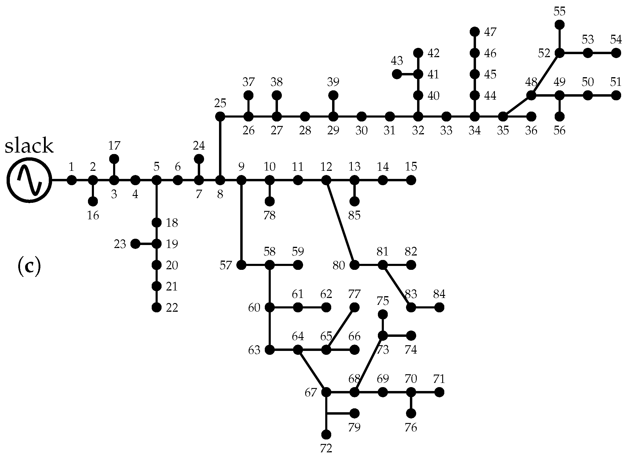
• The IEEE 85-bus test system has 85 buses and 84 transmission lines, as illustrated in Figure 2c. It has a substation at node 1 that works with 11 kV, as well as a peak active and reactive demand of $2570.28+j2622.20$ kVA. The test system’s peak demand, resistance, and reactance values are listed in

  Table 3. Electrical parameters of the IEEE 85-bus network.

  k	m	${\mathit{R}}_{\mathit{km}}$ ($\mathbf{\Omega }$)	${\mathit{x}}_{\mathit{km}}$ ($\mathbf{\Omega }$)	${\mathit{P}}_{\mathit{k}}$ (kW)	${\mathit{Q}}_{\mathit{k}}$ (kW)	k	m	${\mathit{R}}_{\mathit{km}}$ ($\mathbf{\Omega }$)	${\mathit{x}}_{\mathit{km}}$ ($\mathbf{\Omega }$)	${\mathit{P}}_{\mathit{k}}$ (kW)	${\mathit{Q}}_{\mathit{k}}$ (kW)
  1	2	0.108	0.075	0	0	34	44	1.002	0.416	35.28	35.99
  2	3	0.163	0.112	0	0	44	45	0.911	0.378	35.28	35.99
  3	4	0.217	0.149	56	57.13	45	46	0.911	0.378	35.28	35.99
  4	5	0.108	0.074	0	0	46	47	0.546	0.226	14	14.28
  5	6	0.435	0.298	35.28	35.99	35	48	0.637	0.264	0	0
  6	7	0.272	0.186	0	0	48	49	0.182	0.075	0	0
  7	8	1.197	0.820	35.28	35.99	49	50	0.364	0.151	36.28	37.01
  8	9	0.108	0.074	0	0	50	51	0.455	0.189	56	57.13
  9	10	0.598	0.410	0	0	48	52	1.366	0.567	0	0
  10	11	0.544	0.373	56	57.13	52	53	0.455	0.189	35.28	35.99
  11	12	0.544	0.373	0	0	53	54	0.546	0.226	56	57.13
  12	13	0.598	0.410	0	0	52	55	0.546	0.226	56	57.13
  13	14	0.272	0.186	35.28	35.99	49	56	0.546	0.226	14	14.28
  14	15	0.326	0.223	35.28	35.99	9	57	0.273	0.113	56	57.13
  2	16	0.728	0.302	35.28	35.99	57	58	0.819	0.340	0	0
  3	17	0.455	0.189	112	114.26	58	59	0.182	0.075	56	57.13
  5	18	0.820	0.340	56	57.13	58	60	0.546	0.226	56	57.13
  18	19	0.637	0.264	56	57.13	60	61	0.728	0.302	56	57.13
  19	20	0.455	0.189	35.28	35.99	61	62	1.002	0.415	56	57.13
  20	21	0.819	0.340	35.28	35.99	60	63	0.182	0.075	14	14.28
  21	22	1.548	0.642	35.28	35.99	63	64	0.728	0.302	0	0
  19	23	0.182	0.075	56	57.13	64	65	0.182	0.075	0	0
  7	24	0.910	0.378	35.28	35.99	65	66	0.182	0.075	56	57.13
  8	25	0.455	0.189	35.28	35.99	64	67	0.455	0.189	0	0
  25	26	0.364	0.151	56	57.13	67	68	0.910	0.378	0	0
  26	27	0.546	0.226	0	0	68	69	1.092	0.453	56	57.13
  27	28	0.273	0.113	56	57.13	69	70	0.455	0.189	0	0
  28	29	0.546	0.226	0	0	70	71	0.546	0.226	35.28	35.99
  29	30	0.546	0.226	35.28	35.99	67	72	0.182	0.075	56	57.13
  30	31	0.273	0.113	35.28	35.99	68	73	1.184	0.491	0	0
  31	32	0.182	0.075	0	0	73	74	0.273	0.113	56	57.13
  32	33	0.182	0.075	14	14.28	73	75	1.002	0.416	35.28	35.99
  33	34	0.819	0.340	0	0	70	76	0.546	0.226	56	57.13
  34	35	0.637	0.264	0	0	65	77	0.091	0.037	14	14.28
  35	36	0.182	0.075	35.28	35.99	10	78	0.637	0.264	56	57.13
  26	37	0.364	0.151	56	57.13	67	79	0.546	0.226	35.28	35.99
  27	38	1.002	0.416	56	57.13	12	80	0.728	0.302	56	57.13
  29	39	0.546	0.226	56	57.13	80	81	0.364	0.151	0	0
  32	40	0.455	0.189	35.28	35.99	81	82	0.091	0.037	56	57.13
  40	41	1.002	0.416	0	0	81	83	1.092	0.453	35.28	35.99
  41	42	0.273	0.113	35.28	35.99	83	84	1.002	0.416	14	14.28
  41	43	0.455	0.189	35.28	35.99	13	85	0.819	0.340	35.28	35.99

  . These values were taken from [39].

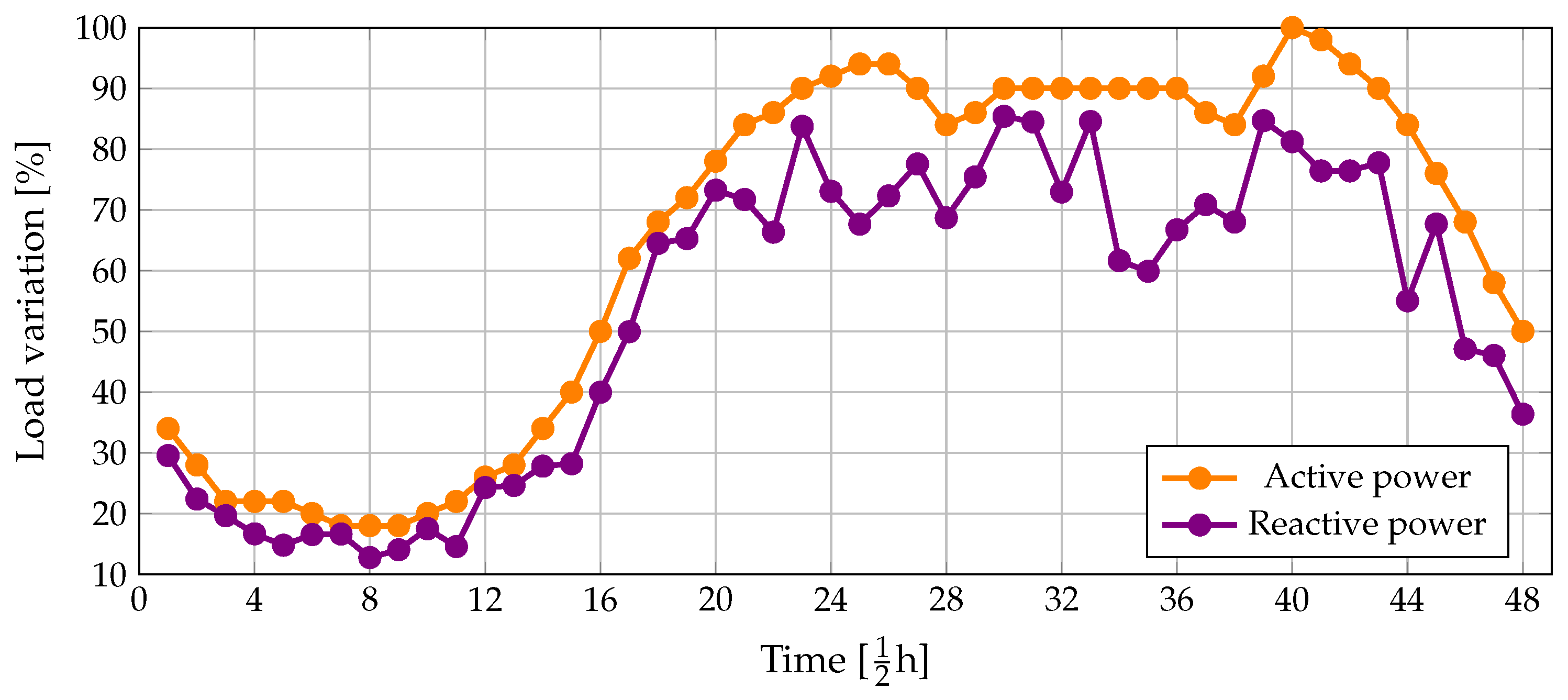
Typically, electrical distribution systems exhibit a daily load variation. The demand curves for the active and reactive power are considered as illustrated in Figure 3. These curves represent the typical behavior of an electrical distribution system in Colombia [40].

The parameter values of the objective function z (1) are shown in

Table 4. Parameter values for the objective functions.

Par.	Value	Unit	Par.	Value	Unit
C	0.1390	USD/kWh	T	365	Days
${\mathsf{\Delta }}_h$	0.50	hour	$k_1$	6/2190	1/Days
$k_2$	10	years	–	–	–
Coefficients of the FACTS devices
Device	${\omega }_1$	Unit	${\omega }_2$	Unit	${\omega }_3$	Unit
SVC	0.30	${\mathrm{USD}/\mathrm{Mvar}}^3$	−305.10	${\mathrm{USD}/\mathrm{Mvar}}^2$	127.380	USD/Mvar
TCSC	1.50	${\mathrm{USD}/\mathrm{Mvar}}^3$	−713.00	${\mathrm{USD}/\mathrm{Mvar}}^2$	153.750	USD/Mvar
UPFC	0.30	${\mathrm{USD}/\mathrm{Mvar}}^3$	−269.10	${\mathrm{USD}/\mathrm{Mvar}}^2$	188.220	USD/Mvar

. The costs associated with the FACTS were taken from [39].

5. Numerical Implementation

The proposed optimization model was implemented in the Yalmip toolbox (R20230622 version) [41], using the Gurobi 9.5.1 solver [42] in the MATLAB 2021a software. A Dell Inspiron 15 7000 Series (Intel Quad-Core i7-7700HQ @2.80 GHz) PC (Dell Inc., Round Rock, TX, USA; Intel Corporation, Santa Clara, CA, USA) with 16 GB RAM and 64-bit Windows 10 Home Single Language (Microsoft Corporation, Redmond, WA, USA) was used to carry out the simulations. Furthermore, the exact optimization model (1)–(16) was also implemented in the GAMS software (23.5.1 version).

The four scenarios shown below were proposed to evaluate the performance of the proposed mixed-integer convex model (25)–(42). All scenarios consider a maximum of three FACTS.

S1:

The proposed model was compared against GAMS, the black widow optimization (BWO) algorithm proposed in [10], and the vortex search algorithm (VSA) presented by [26] for the IEEE 33-bus test system.

S2:

The proposed convex model was evaluated in the IEEE 69-bus test system and compacted to the BWO and VSA, with the aim of installing the SVC devices with a fixed and variable operation.

S3:

The model was evaluated in a large test system, namely the IEEE 85-bus test system. Furthermore, it was compared to the BWO algorithm regarding the installation of SVCs with a fixed and variable operation.

S4:

A comparison regarding the installation of different FACTS technologies was analyzed (i.e., SVC, TCSC, and UPFC devices).

5.1. Analysis of Scenario 1 (S1)

This scenario evaluated and compared the proposed optimization model against the BWO and VSA, and the GAMS software with three different solvers. For this comparison, the installation of only SVC devices was considered.

Table 5. Numerical results of scenario 1.

Method	Location	Size (Mvar)	z (USD/Year)	Reduction [%]
Fixed Operation
Benchmark case	–	–	112,740.90	–
COUENNE	[6, 7, 12]	[0.2693, 0.1646, 0.1932]	104,752.10	7.08
DICOPT	[14, 30, 31]	[0.1598, 0.3496, 0.1165]	98,511.64	12.62
BONMIN	[14, 30, 32]	[0.1599, 0.3591, 0.1072]	98,497.90	12.63
VSA	[14, 30, 32]	[0.1599, 0.3591, 0.1072]	98,497.90	12.63
BWO	[14, 30, 32]	[0.1599, 0.3591, 0.1072]	98,497.90	12.63
Convex model	[14, 30, 32]	[0.1599, 0.3591, 0.1072]	98,497.90	12.63
Variable operation
COUENNE	[6, 7, 12]	[0.2964, 0.1656, 0.2484]	103.945.50	7.80
DICOPT	[14, 30, 32]	[0.1962, 0.4150, 0.3990]	96,676.76	14.24
BONMIN	[14, 30, 32]	[0.1962, 0.4150, 0.3990]	96,676.76	14.24
Convex model	[14, 30, 32]	[0.1962, 0.4150, 0.3990]	96,676.76	14.24

presents the results obtained for the objective function in the radial IEEE 33-bus test system. This scenario was analyzed by considering whether the FACTS-delivered/injected power was fixed or variable during daily operations.

From the results shown in Table 5, it can be stated that:

• The proposed convex model, as well as the BWO and VSA, and the BONMIM solver, reached the best configuration for the SVC devices. This configuration is the global optimum of the problem, as the convex model ensures it. According to the results, node 30 is the most sensitive point of the test system, given that the largest SVC is located in it. This occurs for both the fixed and the variable operation of SVC devices.
• The variable operation of SCV devices reduces the value of the objective function by 14.24%. In contrast, the fixed operation reports a value of 12.63%. This indicates that it is better for the test system to implement a variable operation, as SVCs can inject or absorb reactive power according to the system requirements at each hour of the day. Furthermore, even though the size of the SVCs increases for a variable operation, the objective function value is lower than that of the fixed operation. The total size of the SVC devices for the fixed and variable operation is 0.6262 and 1.0102 Mvar, respectively, increasing the investment costs by 61.17%.

5.2. Analysis of Scenario 2 (S2)

This scenario studied the performance of the proposed optimization model and compares it against that of the BWO and VSA. These algorithms were only used for a fixed operation of the FACTS. In this scenario, no solver of the GAMS reaches convergence. As in the previous scenario, the installation of only SVC devices was considered, given that [10] only analyzes SVCs for the IEEE 69-bus system. The results of the objective function for the IEEE 69-bus test system are shown in

Table 6. Numerical results for scenario 2.

Method	Location	Size [Mvar]	z (USD/Year)	Reduction [%]
Fixed Operation
Benchmark case	–	–	119,715.63	–
VSA	[21, 61, 64]	[0.0839, 0.4601, 0.1139]	102,990.79	13.97
BWO	[21, 61, 64]	[0.0839, 0.4601, 0.1139]	102,990.79	13.97
Convex model	[21, 61, 64]	[0.0839, 0.4601, 0.1139]	102,990.79	13.97
Variable  operation
Convex model	[21, 61, 64]	[0.0929, 0.5774, 0.1481]	100,806.50	15.79

, considering the fixed or variable operation of SVC devices during the day.

From the results obtained in Table 6, note that:

• The solutions found by the BWO and VSA in [10,26] are the global optimum of the problem as the proposed convex model achieves the same configuration. Still, it is essential to note that the proposed convex model will always find the same values, while the BOW and VSA cannot guarantee these results. Furthermore, these algorithms require tuning many parameters, which can affect their performance.
• According to the results obtained for the IEEE 69-bus test system, the node with the highest sensitivity is node 61, as it was selected to install the SVC device with the highest capacity. This behavior is the same for the fixed and variable SVC operations.
• The optimal integration of SVC devices reduces the annual energy losses costs. This reduction is greater for the variable operation. These devices report reductions of 13.97% and 15.79% in the objective functions for the fixed and variable operation. The latter saves USD 3778.4/year more than the former. Despite this, the total size of the SVCs increases by 24.35% for the variable operation.

5.3. Analysis of Scenario 3 (S3)

This scenario evaluated the performance of the proposed optimization model in a large electrical distribution network, such as the IEEE 85-bus test system. Furthermore, the model was compared to the BWO algorithm, which was designed exclusively for the fixed operation of FACTS. Only SVC devices were considered for installation (see the literature reference [10]). The results regarding their location and size, as well as the objective function values and their reduction, are listed in

Table 7. Numerical results for scenario 3.

Method	Location	Size [Mvar]	z (USD/Year)	Reduction [%]
Fixed Operation
Benchmark case	–	–	154,651.95	–
BWO	[12, 34, 67]	[0.2490, 0.3930, 0.3289]	113,619.97	26.53
Fixed Operation
Convex model	[12, 34, 67]	[0.2490, 0.3930, 0.3289]	113,619.97	26.53
Variable operation
Convex model	[12, 34, 67]	[0.3094, 0.5085, 0.4221]	107,777.80	30.31

for this test system.

From Table 7, it can be stated that:

• The proposed convex model and the BWO algorithm reach the best configuration with regard to the SVC devices, which constitutes the global solution to the problem. All SVC devices in the IEEE 85-bus test system are located in nodes with bifurcations. This behavior is different in the other two test systems. However, these locations are expected given the characteristics of the IEEE 85-bus grid, i.e., its many circuit branches, distribution of loads, and large size.
• The SVC device with the highest capacity was installed at node 61. However, unlike the other two test systems, this one did not report a node with heightened sensitivity, since there was no significant difference between the two largest SVCs installed.
• The annual energy losses costs are reduced with the installation of SVCs. This reduction is significant for the variable operation. The reductions in the objective functions for the fixed and variable operation of the devices are 26.53% and 30.31%, respectively. This implies that the variable operation saves USD 9251.81/year more than the other.

5.4. Analysis of Scenario 4 (S4)

This scenario analyzes the impact of installing different FACTS technologies on the test systems, namely the SVC, TCSC, and UPFC devices. This analysis and comparison only consider a variable operation.

Table 8. Numerical results for scenario 4.

FACTS Devices	Location	Size [Mvar]	z (USD/Year)	Reduction [%]
IEEE 33-Bus Test System
Benchmark case	–	–	112,740.90	–
UPFC	[14, 30, 32]	[0.1569, 0.3486, 0.1364]	101,078.70	10.34
TCSC	[14, 30, 32]	[0.1786, 0.4022, 0.1365]	98,729.21	12.42
SVC	[14, 30, 32]	[0.1962, 0.4150, 0.3990]	96,676.76	14.24
IEEE 69-bus test system
Benchmark case	–	–	119,715.63	–
UPFC	[21, 61, 64]	[0.0403, 0.4811, 0.1456]	105,316.40	12.03
TCSC	[21, 61, 64]	[0.0683, 0.5380, 0.1450]	102,861.80	14.07
SVC	[21, 61, 64]	[0.0929, 0.5774, 0.1481]	100,806.50	15.79
IEEE 85-bus test system
Benchmark case	–	–	154,651.95	–
UPFC	[12, 34, 67]	[0.2483, 0.4770, 0.3836]	114,920.20	25.69
TCSC	[12, 34, 67]	[0.2820, 0.4951, 0.4055]	110,951.00	28.25
SVC	[12, 34, 67]	[0.3094, 0.5085, 0.4221]	107,777.80	30.31

presents the results obtained for the objective function as well as the location and size of the FACTS for all test systems. These results only pertain to the proposed convex model, as it guarantees the global optimum of the problem.

From Table 8, the following remarks can be made:

• The nodes found for locating the different types of FACTS are the same in all test systems. This means that these nodes are more sensitive to reducing the costs of energy losses by injecting or absorbing reactive power. SVC devices maintain the same behavior in all test systems, reducing the costs of energy losses to a greater extent.
• For the IEEE 33-bus test system, the annual operating costs were minimized to values ranging from USD 101,078.70 (for installed UPFC devices) to USD 96,676.76 (for installed SVCs). The reductions in the objective function were 10.34%, 12.42%, and 14.24% for the UPFC, TCSC, and SVC devices, respectively.
• For the IEEE 69-bus test system, the annual equivalent operating costs were reduced to values ranging from USD 105,316.40 (for installed UPFC devices) to USD 100,806.50 (for installed SVCs). The objective function was reduced by 12.03%, 14.07%, and 15.79% with respect to the benchmark case (i.e., the case without FACTS integration) for the UPFC, TCSC, and SVC devices, respectively.
• For the IEEE 85-bus test system, the annual energy loss costs decreased to values ranging from USD 114,920.20 (for installed UPFC devices) to USD 107,777.80 (for installed SVCs). The annual equivalent operating costs were reduced by 25.69%, 28.25%, and 30.31% with respect to the benchmark case for the UPFC, TCSC, and SVC devices, respectively.

6. Conclusions and Future Works

This paper addressed the optimal integration of FACTS in electrical distribution grids, considering the minimization of the annual costs related to energy losses and the investments made in installing these devices. This integration was solved using a mixed-integer convex model, which was obtained by transforming the hyperbolic constraints of the MINLP model into second-order conic constraints. The effectiveness of our proposal was evaluated in three IEEE test systems, and it was compared to the BWO and VSA and some GAMS software solvers. The results showed that the proposed convex model found the global optimum of the studied problem. Fixed and variable operations were considered for the FACTS. For the fixed operation, the annual operating costs were reduced by 12.63%, 13.97%, and 26.53% for the IEEE 33-, 69-, and 85-bus test systems, respectively. These results were achieved by the proposed convex model and the BWO algorithm; the other solvers sometimes failed to converge or reached a worse solution. For the variable operation of SVC devices, the annual equivalent operating costs were reduced by 14.24%, 15.79%, and 30.31% for the IEEE 33-, 69-, and 85-bus test systems, respectively. These results were also achieved by the proposed convex model and the BWO algorithm.

The variable operation of SVC devices allowed for a more significant reduction in the annual energy losses costs, although the total size of the SVCs increased by 61.17%, 24.35%, and 27.71% for the IEEE 33-, 69-, and 85-bus test systems, respectively. However, this saved USD 6693.3, 3778.4, and 3778.4/year more than the fixed operation.

The installation of SVC devices was the best option to reduce the final objective function value in all test systems. The second best option was TCSC devices. The total size of the SVCs was greater in all test systems than the other FACTS, thus enabling a greater reserve of reactive power as demand grows.

References

- Wagle, R.; Sharma, P.; Sharma, C.; Amin, M. Optimal power flow based coordinated reactive and active power control to mitigate voltage violations in smart inverter enriched distribution network. Int. J. Green Energy 2023, 1–17. [Google Scholar] [CrossRef]
- Kawasaki, S.; Suzuki, K. A Study on Improvement of Power Quality by STATCOMs for Low Voltage System. J. Int. Counc. Electr. Eng. 2019, 9, 93–104. [Google Scholar] [CrossRef][Green Version]
- Zamani, A.; Sidhu, T.; Yazdani, A. A strategy for protection coordination in radial distribution networks with distributed generators. In Proceedings of the IEEE PES General Meeting, Minneapolis, MN, USA, 25–29 July 2010. [Google Scholar] [CrossRef]
- Montoya, O.D.; Serra, F.M.; Angelo, C.H.D.; Chamorro, H.R.; Alvarado-Barrios, L. Heuristic Methodology for Planning AC Rural Medium-Voltage Distribution Grids. Energies 2021, 14, 5141. [Google Scholar] [CrossRef]
- Hijazi, H.; Thiébaux, S. Optimal distribution systems reconfiguration for radial and meshed grids. Int. J. Electr. Power Energy Syst. 2015, 72, 136–143. [Google Scholar] [CrossRef]
- Wang, Y.; Tan, K.T.; Peng, X.Y.; So, P.L. Coordinated Control of Distributed Energy-Storage Systems for Voltage Regulation in Distribution Networks. IEEE Trans. Power Deliv. 2016, 31, 1132–1141. [Google Scholar] [CrossRef]
- Alyu, A.B.; Salau, A.O.; Khan, B.; Eneh, J.N. Hybrid GWO-PSO based optimal placement and sizing of multiple PV-DG units for power loss reduction and voltage profile improvement. Sci. Rep. 2023, 13, 6903. [Google Scholar] [CrossRef]
- Valencia, A.; Hincapie, R.A.; Gallego, R.A. Optimal location, selection, and operation of battery energy storage systems and renewable distributed generation in medium–low voltage distribution networks. J. Energy Storage 2021, 34, 102158. [Google Scholar] [CrossRef]
- Nanibabu, S.; Shakila, B.; Prakash, M. Reactive Power Compensation using Shunt Compensation Technique in the Smart Distribution Grid. In Proceedings of the 2021 6th International Conference on Computing, Communication and Security (ICCCS), Las Vegas, NV, USA, 4–6 October 2021. [Google Scholar] [CrossRef]
- Santamaria-Henao, N.; Montoya, O.D.; Trujillo-Rodríguez, C.L. Optimal Siting and Sizing of FACTS in Distribution Networks Using the Black Widow Algorithm. Algorithms 2023, 16, 225. [Google Scholar] [CrossRef]
- Shaheen, A.M.; El-Sehiemy, R.A.; Ginidi, A.; Elsayed, A.M.; Al-Gahtani, S.F. Optimal Allocation of PV-STATCOM Devices in Distribution Systems for Energy Losses Minimization and Voltage Profile Improvement via Hunter-Prey-Based Algorithm. Energies 2023, 16, 2790. [Google Scholar] [CrossRef]
- Lakshmi, S.; Ganguly, S. Transition of Power Distribution System Planning from Passive to Active Networks: A State-of-the-Art Review and a New Proposal. In Sustainable Energy Technology and Policies; Springer: Singapore, 2017; pp. 87–117. [Google Scholar] [CrossRef]
- Elsheikh, A.; Helmy, Y.; Abouelseoud, Y.; Elsherif, A. Optimal capacitor placement and sizing in radial electric power systems. Alex. Eng. J. 2014, 53, 809–816. [Google Scholar] [CrossRef]
- Marouani, I.; Guesmi, T.; Alshammari, B.M.; Alqunun, K.; Alshammari, A.S.; Albadran, S.; Abdallah, H.H.; Rahmani, S. Optimized FACTS Devices for Power System Enhancement: Applications and Solving Methods. Sustainability 2023, 15, 9348. [Google Scholar] [CrossRef]
- Eid, A.; Kamel, S.; Abdel-Mawgoud, H. Shunt Reactive Compensations for Distribution Network Optimization. In Advanced Control & Optimization Paradigms for Energy System Operation and Management; River Publishers: Aalborg, Denmark, 2023; pp. 109–135. [Google Scholar] [CrossRef]
- Gandoman, F.H.; Ahmadi, A.; Sharaf, A.M.; Siano, P.; Pou, J.; Hredzak, B.; Agelidis, V.G. Review of FACTS technologies and applications for power quality in smart grids with renewable energy systems. Renew. Sustain. Energy Rev. 2018, 82, 502–514. [Google Scholar] [CrossRef]
- Ara, A.L.; Kazemi, A.; Niaki, S.A.N. Multiobjective Optimal Location of FACTS Shunt-Series Controllers for Power System Operation Planning. IEEE Trans. Power Deliv. 2012, 27, 481–490. [Google Scholar] [CrossRef]
- Gil-González, W. Optimal Placement and Sizing of D-STATCOMs in Electrical Distribution Networks Using a Stochastic Mixed-Integer Convex Model. Electronics 2023, 12, 1565. [Google Scholar] [CrossRef]
- Saghand, P.G.; Charkhgard, H. Exact solution approaches for integer linear generalized maximum multiplicative programs through the lens of multi-objective optimization. Comput. Oper. Res. 2022, 137, 105549. [Google Scholar] [CrossRef]
- Reddy, S.G.; Ganapathy, S.; Manikandan, M. Power quality improvement in distribution system based on dynamic voltage restorer using PI tuned fuzzy logic controller. Electr. Eng. Electromech. 2022, 1, 44–50. [Google Scholar] [CrossRef]
- Biswas, P.P.; Arora, P.; Mallipeddi, R.; Suganthan, P.N.; Panigrahi, B.K. Optimal placement and sizing of FACTS devices for optimal power flow in a wind power integrated electrical network. Neural Comput. Appl. 2020, 33, 6753–6774. [Google Scholar] [CrossRef]
- Turgut, M.S.; Turgut, O.E.; Afan, H.A.; El-Shafie, A. A novel Master–Slave optimization algorithm for generating an optimal release policy in case of reservoir operation. J. Hydrol. 2019, 577, 123959. [Google Scholar] [CrossRef]
- Mistry, M.; Letsios, D.; Krennrich, G.; Lee, R.M.; Misener, R. Mixed-Integer Convex Nonlinear Optimization with Gradient-Boosted Trees Embedded. INFORMS J. Comput. 2021, 33, 1103–1119. [Google Scholar] [CrossRef]
- Varma, R.K.; Siavashi, E.M.; Mohan, S.; Vanderheide, T. First in Canada, Night and Day Field Demonstration of a New Photovoltaic Solar-Based Flexible AC Transmission System (FACTS) Device PV-STATCOM for Stabilizing Critical Induction Motor. IEEE Access 2019, 7, 149479–149492. [Google Scholar] [CrossRef]
- Raj, S.; Bhattacharyya, B. Optimal placement of TCSC and SVC for reactive power planning using Whale optimization algorithm. Swarm Evol. Comput. 2018, 40, 131–143. [Google Scholar] [CrossRef]
- Montoya, O.D.; Gil-González, W.; Hernández, J.C. Efficient Operative Cost Reduction in Distribution Grids Considering the Optimal Placement and Sizing of D-STATCOMs Using a Discrete-Continuous VSA. Appl. Sci. 2021, 11, 2175. [Google Scholar] [CrossRef]
- Sirjani, R.; Jordehi, A.R. Optimal placement and sizing of distribution static compensator (D-STATCOM) in electric distribution networks: A review. Renew. Sustain. Energy Rev. 2017, 77, 688–694. [Google Scholar] [CrossRef]
- Gupta, A.R.; Kumar, A. Optimal placement of D-STATCOM using sensitivity approaches in mesh distribution system with time variant load models under load growth. Ain Shams Eng. J. 2018, 9, 783–799. [Google Scholar] [CrossRef]
- de Koster, O.A.C.; Domínguez-Navarro, J.A. Multi-Objective Tabu Search for the Location and Sizing of Multiple Types of FACTS and DG in Electrical Networks. Energies 2020, 13, 2722. [Google Scholar] [CrossRef]
- Mori, H.; Tani, H. A Tabu Search Based Method for Optimal Allocation of D-FACTS in Distribution Systems. IFAC Proc. Vol. 2008, 41, 14951–14956. [Google Scholar] [CrossRef]
- Reddy, G.H.; Koundinya, A.N.; Gope, S.; Raju, M.; Singh, K.M. Optimal Sizing and Allocation of DG and FACTS Device in the Distribution System using Fractional Lévy Flight Bat Algorithm. IFAC-PapersOnLine 2022, 55, 168–173. [Google Scholar] [CrossRef]
- Ravi, K.; Rajaram, M. Optimal location of FACTS devices using Improved Particle Swarm Optimization. Int. J. Electr. Power Energy Syst. 2013, 49, 333–338. [Google Scholar] [CrossRef]
- Pappachan, S.N. Development of optimal placement and sizing of FACTS devices in power system integrated with wind power using modified krill herd algorithm. COMPEL Int. J. Comput. Math. Electr. Electron. Eng. 2023. [Google Scholar] [CrossRef]
- Sulaiman, M.H.; Mustaffa, Z. Optimal placement and sizing of FACTS devices for optimal power flow using metaheuristic optimizers. Results Control Optim. 2022, 8, 100145. [Google Scholar] [CrossRef]
- Saravan, M.; Slochanal, S.; Venkatesh, P.; Abraham, P. Application of PSO technique for optimal location of FACTS devices considering system loadability and cost of installation. In Proceedings of the 2005 International Power Engineering Conference, Singapore, 29 November–2 December 2005. [Google Scholar] [CrossRef]
- Montoya, O.D.; Garces, A.; Gil-González, W. Minimization of the distribution operating costs with D-STATCOMS: A mixed-integer conic model. Electr. Power Syst. Res. 2022, 212, 108346. [Google Scholar] [CrossRef]
- Zohrizadeh, F.; Josz, C.; Jin, M.; Madani, R.; Lavaei, J.; Sojoudi, S. A survey on conic relaxations of optimal power flow problem. Eur. J. Oper. Res. 2020, 287, 391–409. [Google Scholar] [CrossRef]
- Lavaei, J.; Tse, D.; Zhang, B. Geometry of Power Flows and Optimization in Distribution Networks. IEEE Trans. Power Syst. 2014, 29, 572–583. [Google Scholar] [CrossRef]
- Montoya, O.D.; Gil-González, W.; Hernández, J.C. Efficient Integration of Fixed-Step Capacitor Banks and D-STATCOMs in Radial and Meshed Distribution Networks Considering Daily Operation Curves. Energies 2023, 16, 3532. [Google Scholar] [CrossRef]
- Montoya, O.D.; Gil-González, W. Dynamic active and reactive power compensation in distribution networks with batteries: A day-ahead economic dispatch approach. Comput. Electr. Eng. 2020, 85, 106710. [Google Scholar] [CrossRef]
- Lofberg, J. YALMIP: A toolbox for modeling and optimization in MATLAB. In Proceedings of the 2004 IEEE International Conference on Robotics and Automation (IEEE Cat. No. 04CH37508), Taipei, Taiwan, 2–4 September 2004; pp. 284–289. [Google Scholar]
- Gurobi Optimization, LLC. Gurobi Optimizer Reference Manual; Gurobi Optimization, LLC: Beaverton, OR, USA, 2022. [Google Scholar]