Using Epidemiological Models to Predict the Spread of Information on Twitter

Abstract

In this article, we analyze the spread of information on social media (Twitter) and purpose a strategy based on epidemiological models. It is well known that social media represent a strong tool to spread news and, in particular, fake news, due to the fact that they are free and easy to use. First, we propose an algorithm to create a proper dataset in order to employ the ignorants–spreaders–recovered epidemiological model. Then, we show that to use this model to study the diffusion of real news, parameter estimation is required. We show that it is also possible to accurately predict the evolution of news spread and its peak in terms of the maximum number of people who share it and the time when the peak occurs trough a process of data reduction, i.e., by using only a part of the built dataset to optimize parameters. Numerical results based on the analysis of real news are also provided to confirm the applicability of our proposed model and strategy.

1. Introduction

Social media have become a great tool for the dissemination of information, especially if we consider the dissemination of fake news. They are easy to use and free, and for this reason, in some cases, they are the main source of information. Therefore, it is important to understand not only how news spreads on social media but also the period of time when a news story is popular or the moment when the peak of maximum popularity of the news item occurs. For example, for a company that produces technological devices, it can be advantageous to predict when there will be maximum interest in a topic on social networks in order to launch a new product at the right time, maximizing earnings. Similarly, with respect to fake news, these factors are also fundamental, since predicting the peak of diffusion of fake news allows us to apply countermeasures to block such content (see more details in [1]). Fake news can be crucial for the outcome of some political decisions or social events, such as the American presidential elections of 2016 or Brexit, as shown in [2]; therefore, a good way of analyzing fake news is required.

Several models are available to study the spread of information, including suitable epidemiological models based on ordinary differential equations [3,4,5,6,7,8,9,10,11,12,13], models based on partial differential equations [14,15,16,17,18] and models based on stochastic differential equations [19,20,21]. In this work, in particular, we consider models based on ordinary differential equation systems that are also used in mathematical epidemiology to study the spread of an epidemic (for more epidemiological models and details of models used in mathematical epidemiology, see [22]). Research activity on epidemiological models is widespread and does not only concern the construction of models capable of characterizing the actual spread of epidemics but also the derivation of numerical methods that are able to preserve the fundamental features of the related exact solution, such as the equilibrium point properties, are important for locating and analyzing peaks; positivity [23,24,25,26,27]; the oscillation frequency (if any) [28,29]; and inherent conservation laws [30,31,32].

In mathematical epidemiology, there are different kinds of models based on ordinary differential equation systems, including:

• “Ode systems-based models” that divide the population into different classes named according to the state in which various individuals find themselves, such as susceptible, infected, dead, recovered, etc. Each equation of the system describes the evolution of these classes;
• Stochastic models that use stochastic differential equation systems;
• Models with delay that use delayed differential equations in order to consider the incubation period of a virus.

In this paper, we consider models of the first class by treating news as a virus and studying its evolution through ordinary differential equations systems. Consequently, to archive our goal of predicting the trend of news and its peak, we have to find both the right model and the best possible set of parameters for it in order to obtain the most realistic result that fits the real data that we collected from social media site “Twitter” using the tools shown in the next section. Moreover, we also want to understand if there are some common points that characterize the diffusion of different kinds of news. One relevant aspect to take into consideration, as underlined in [2], is that a key role is played by the grade of access to the Internet of the population. Countries with the highest grade are more vulnerable to the spread of fake news. However, this cannot be the only reason. There are also other important factors, such as the person (or the group of persons) who shares the news first or the period of time when the news is popular, which could have a considerable impact on the grade of the news diffusion, as we show in the section dedicated to numerical experiments.

The paper is organized as follows. In Section 2, we present some epidemiology-based information spread models in order to describe the model that we propose and the reasons behind this choice. In Section 3, we explain the materials and methods used for data acquisition and numerical tests, starting with an explanation of why we decided to analyze Twitter and not another social network. Moreover, we provide a brief description of the main news that we followed and analyzed, and we also propose strategies to obtain optimized parameters. In Section 4, we present the main outcomes of numerical experiments and a brief discussion thereof, confirming our thesis, while the final Section comprises concluding remarks.

2. Epidemiology-Based Information Spread Models

As anticipated, there are different ways to study the spread of information on social networks, among which we considered the epidemiological ones. From a mathematical point of view, there is an analogy between describing the evolution of an epidemic and the process of dissemination of information. An epidemic spreads by affecting the majority of the population, (as occurred, for example, with the COVID-19 pandemic in 2020); likewise, news can be compared to a contagious virus spread by all those who share it on social networks. We consider epidemiological models based on $OD{E}_S$ systems that study epidemics by dividing population in different classes. Such models comprise different types: from the easiest one, the SI (susceptible–infected) model, that takes into consideration only susceptible individuals who can be infected and infected individuals (see [22] for more details), to more complex models that involve dead, recovered, hospitalized and quarantined individuals, etc. With the aim of studying information diffusion on the web or on social media, we chose classes of individuals taking into account the available data in order to validate the model using real data.

Hence, we focused on models that were developed to study epidemics but that can be easily adapted to describe the dissemination of information or models that have some characteristics in common with epidemic models but that were developed explicitly to study information spread, i.e., the ISR (ignorants spreaders recovered) model and the IESZ (ignorants exposed spreaders skeptics) model ([10,11,12,33]). Before introducing these two models, a brief explanation of the terminology used in this paper is required.

In epidemiology, there is a lot of models with similar names, such as the SIR (susceptible infected recovered) model introduced in 1927 by Kermack and McKendrick in their work called “A contribution to the mathematical theory of epidemics”. However, here, the notation is different. In the case of the SIR model, the population is divided into three different classes, which are described as follows:

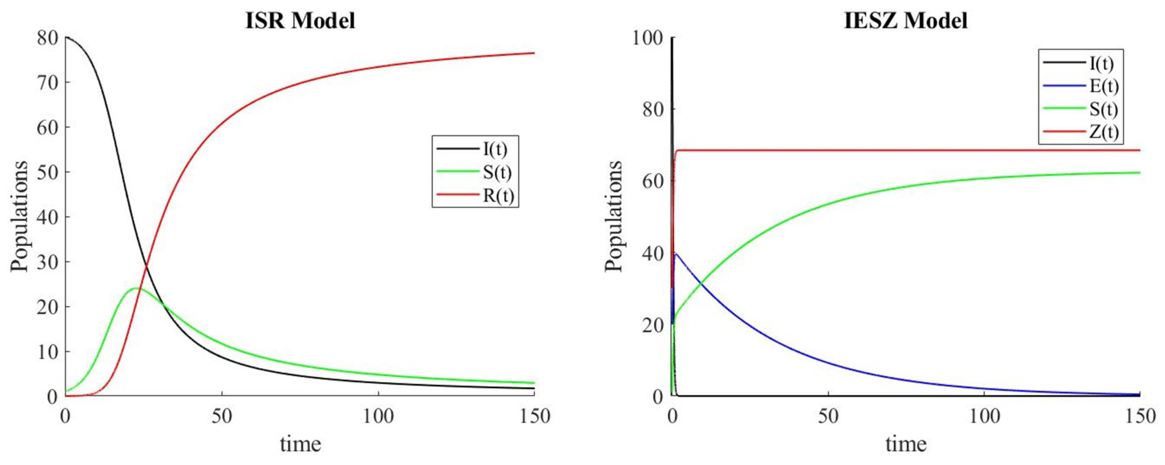
• S(t), i.e., susceptible class: the class of people who can be infected;
• I(t), i.e., infectious class: the class of people who are infected;
• R(t), i.e., recovered class: the class of people who have recovered from disease.

In our case, although we can use the word “susceptible” to refer people who can see a tweet containing news, the word “infectious” to refer to people who saw the news and decided to share it, and the word “recovered” to refer to people who recovered because they lost their interest in the news or because they do not believe in that news anymore. It is more appropriate to apply some changes to the notation by considering the ISR model, which refers to three different classes of the population as follows:

• I(t), i.e, ignorant class. This group plays the role the susceptible class, because its members are all users of the social network who can see the news, but  they have not seen it yet, so they ignore it;
• S(t), i.e, spreader class. This group plays the role of the infectious class because its members are the users that spread the news, exactly as infected individuals can spread a disease during an epidemic;
• R(t), i.e, recovered class. This group plays the role of the recovered class, such as in the SIR model of epidemics; they are individuals who do not spread the news anymore.

Using the previous notation, we introduce the following parameters:

• $\beta$: the news spreading rate;
• $\gamma$: the recovery rate;
• k: the average number of connections among individuals;
• N: the population size.

The model is obtained as follows [11]:

$$\begin{array}{c}\hfill \left\{\begin{array}{c}{I}^{\prime }\left(t\right)=-\frac{\beta kI\left(t\right)S\left(t\right)}{N}\hfill \\ S^{\prime }\left(t\right)=\frac{\beta kI\left(t\right)S\left(t\right)}{N}-\frac{\gamma kS\left(t\right)S\left(t\right)}{N}\hfill \\ R^{\prime }\left(t\right)=\frac{\gamma kS\left(t\right)S\left(t\right)}{N}\hfill \end{array}\right.\end{array}$$

(1)

The dynamics of interactions of the three classes of the population are represented by the following graph (Figure 1):

As we previously anticipated, there are many other models that can be used to describe news spread. An example is the IESZ model, which, contrary to the ISR model, was developed to study the spread of information, although it is an ODE system-based model, like the previously discussed model.

It divides the population into four classes as follows:

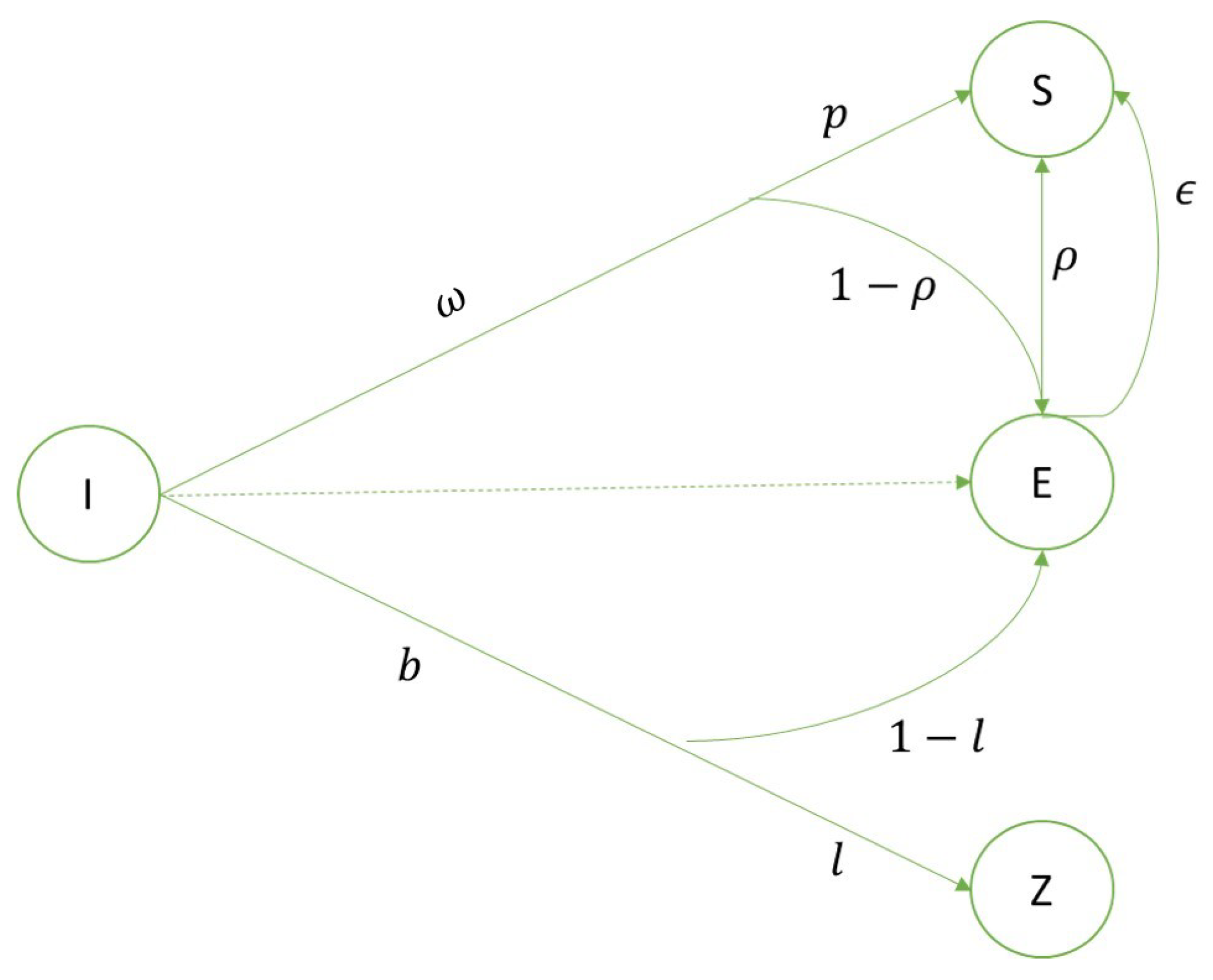
• I(t), i.e., ignorant class. As in the ISR model, this group represents the class of people that can see the news;
• E(t), i.e., exposed class. The class of people who have been exposed to the news but have not yet shared it;
• S(t), i.e., spreader class. The class of people who spread the news;
• Z(t), i.e., skeptic class. The class of people who saw the news but choose to ignore it.

As before, to formulate the model, we have to introduce some parameters, taking into account that a “contact” between two individuals occurs when one of them reads a tweet or a comment of the other. Therefore, we introduce:

• $\omega$: the contact rate between a member of the ignorant class and a member of the spreader class;
• b: the contact rate between a member of the ignorant class and a member of the skeptic class;
• p: the probability of transition from the ignorants class to the spreader class after a meeting between a member of the former class with a member of the latter class;
• l: the probability of transition from the ignorants class to the skeptic class;
• $\rho$: the contact rate between a member of the exposed class and a member of the spreader class;
• $ϵ$: the transition rate from the exposed class to the spreader class;
• N: population size, which is the sum of the sizes of each class.

The following graph (Figure 2) summarizes all the parameters and the possible transitions from one class to another.

The model is obtained as follows [10]:

$$\begin{array}{c}\hfill \left\{\begin{array}{c}{I}^{\prime }\left(t\right)=-\frac{\omega IS}{N}-b\frac{IZ}{N}\hfill \\ E^{\prime }\left(t\right)=(1-p)\omega \frac{IS}{N}+(1-l)b\frac{IZ}{N}-\rho E\frac{S}{N}-ϵE\hfill \\ S^{\prime }\left(t\right)=\frac{p\omega IS}{N}+\rho E\frac{S}{N}+ϵE\hfill \\ Z^{\prime }\left(t\right)=lbI\frac{Z}{N}\hfill \end{array}\right.\end{array}$$

(2)

As we can see, there is not a direct transition from the class of ignorants to the class of exposed individuals. In fact, a member of the class of ignorants can see the news in the form of a tweet; then, he can encounter a member of the class of spreaders and become exposed with a probability of $(1-p)$ if he does not share the news, or he can become a spreader himself if he chooses to share the news, with a probability of p. On the contrary, if he reads the news but does not show any particular reaction, he transitions to the skeptic class, with a probability of l, while if he believes in the news, even after a period of time but he does not share it, he passes to the exposed class, with a probability of $(1-l)$.

An application of these two models can be seen in Figure 3, where, on the left, we report the plot of the solution of model (1) in correspondence with example parameters:

$$\beta =0.2;\gamma =0.3;\kappa =1.2$$

(3)

while on the right, we present the solution of model (2) in correspondence with example parameters:

$$\omega =4.3;b=8;p=0.7;l=0.8;\rho =1.38\times {10}^{-6};ϵ=0.03;$$

(4)

We observe that the two models are very different. Not only the dynamics differ among the different populations, but the results that we obtain if we use the two models to predict the evolution of a news item also differ. Indeed, the ISR Model foresees the transition from the class of ignorants to that of spreaders, then to that of recovered, so the spreaders function (S(t)) is, at first, an increasing function; then, it reaches a maximum inside the interval under consideration, and finally, it decreases. This characteristic of the model allows us to predict the peak of the spread, enabling a quantitative estimation of the period of time when the news is popular. Instead, the IESZ model considers only transitions from the exposed or ignorant class to the spreader class and from the ignorant class to the skeptic class. Therefore, someone who is a spreader will remain in this class forever, and S(t) is an increasing function. For this reason, this kind of model can be used to describe news that is popular for a short period of time, but it is not suitable for making the predictions we are interested in.

There is also another disadvantage of the IESZ Model. Using the tools described in Section 3, after obtaining data from Twitter related to users who have shared a particular news item in a given time interval, we have to organize them creating the different classes that we want to analyze. Given a finite number of instances of time in the assigned time interval, it is possible to construct vectors containing the number of individuals belonging to each of the classes, such as ignorants, spreaders or recovered, but this is not possible for the exposed class, which is the class of people who saw the tweet containing the news but who have not shared it yet. It is not possible to establish exactly how many people are in this class. The same disadvantage occurs for other models, such as the SEIR model (IESR if we want to use the new notation) of epidemics that considers the classes of susceptible, infectious, exposed and recovered individuals. Other models, such as the ISI model (ignorants spreaders ignorants model) or the ISRI model (ignorants spreaders recovered ignorants model), require a long observation period, so they are recommended for periodical news, but they are not useful for news that spreads only once [3]. For all these reasons, we decided to focus our attention on the the ISR model.

3. Data Acquisition and Parameter Estimation

In order to analyze the diffusion of information on social media, as a first step, we collected real data. Unlike other scientific fields, where there datasets are organized and directly available on the Web, in this case, we obtained these data from a chosen social network; in particular, we focused our work on Twitter. The motivation of this choice relies on the fact that it is possible to collect data by using tools such as the official Twitter portal called the “Twitter Developer Option” [34] and Python data scraper “Tweepy” [35]. In this way, we obtained information of different kinds about Twitter users who shared the searched news item, such as Twitter ID, mentions, Twitter username, the number of followers, etc. In particular, for the work that we describe herein, we needed the date of creation of the tweet in which we were interested and the username of the users who posted it. We analyzed the diffusion of a news item by following the trends of a “hashtag”. Data analysis was performed by searching for news with a specific hashtag or with a specific group of keywords. This aspect can be improved, as in some cases, there are tweets with a particular hashtag whose topic is not related to the hashtag itself. After collecting data, starting from the algorithm described in [11,12], we wrote an algorithm, which is reported as Algorithm 1, that allowed us to classify individuals as ignorants, spreaders or recovered.

Algorithm 1 Constructing ISR vectors from Twitter data.

1: $I\leftarrow IgnorantPopulation$ 2: $S\leftarrow SpreaderPopulation$ 3: $R\leftarrow RecoveredPopulation$ 4: $t\leftarrow FirstDataofdataset$ 5: $t_{end}\leftarrow LastDataofdataset$ 6: $t_{exit}\leftarrow Timetopassfromspreaderstorecovered$ 7: for each user do 8:     $t_0\leftarrow firsttimethisusertweeted$ 9:     $t_1\leftarrow lasttimethisusertweeted$ 10: end for 11: loop 12: if$t\le t_0$then 13:     $I\leftarrow I+1$ 14:     $t\leftarrow t+t_{exit}$ 15:     go to loop 16: else 17:     if $t_0\le t\le t_1+t_{exit}$ then 18:         $S\leftarrow S+1$ 19:         $t\leftarrow t+t_{exit}$ 20:         go to loop 21:     else 22:         if $t_1\le t\le t_{end}+t_{exit}$ then 23:            $R\leftarrow R+1$ 24:            $t\leftarrow t+t_{exit}$ 25:            go to loop 26:         else 27:            close loop 28:         end if 29:     end if 30: end if

In particular, the algorithm puts each user is in the ignorant class before the time instant ($t_0$) in which he publishes his first tweet. At this point, the user becomes part of the class of spreaders. $t_1$ denotes the time instant at which the user publishes their last tweet relating to the news under consideration. The user passes into the recovered class at time instant $t_1+t_{exit}$. As readers can imagine, the time required to pass from one compartment to another ($t_{exit}$) depends on the news that we are following. To build the dataset, it is necessary to organize data using different transition times from the state of spreader to recovered.

For our research purposes, $t_{exit}$ was empirically selected through a series of tests by taking the following factors into account:

• News popularity: the degree of popularity or attention received by the news;
• Time range: the duration of time taken into consideration;
• Number of tweets posted within the selected time range;
• The level of influence or popularity of users within the network who share the analyzed news.

3.1. Case Studies

First of all, let us introduce and provide some details about the news that we analyzed. We considered different kinds of news or rumors related to different topics that have trended during the last two years (during different periods of time) so that the of number of corresponding tweets to be analyzed was sufficiently high to justify modeling through an epidemiological model.

In particular, we analyzed trends that are news or rumors related to the following topics:

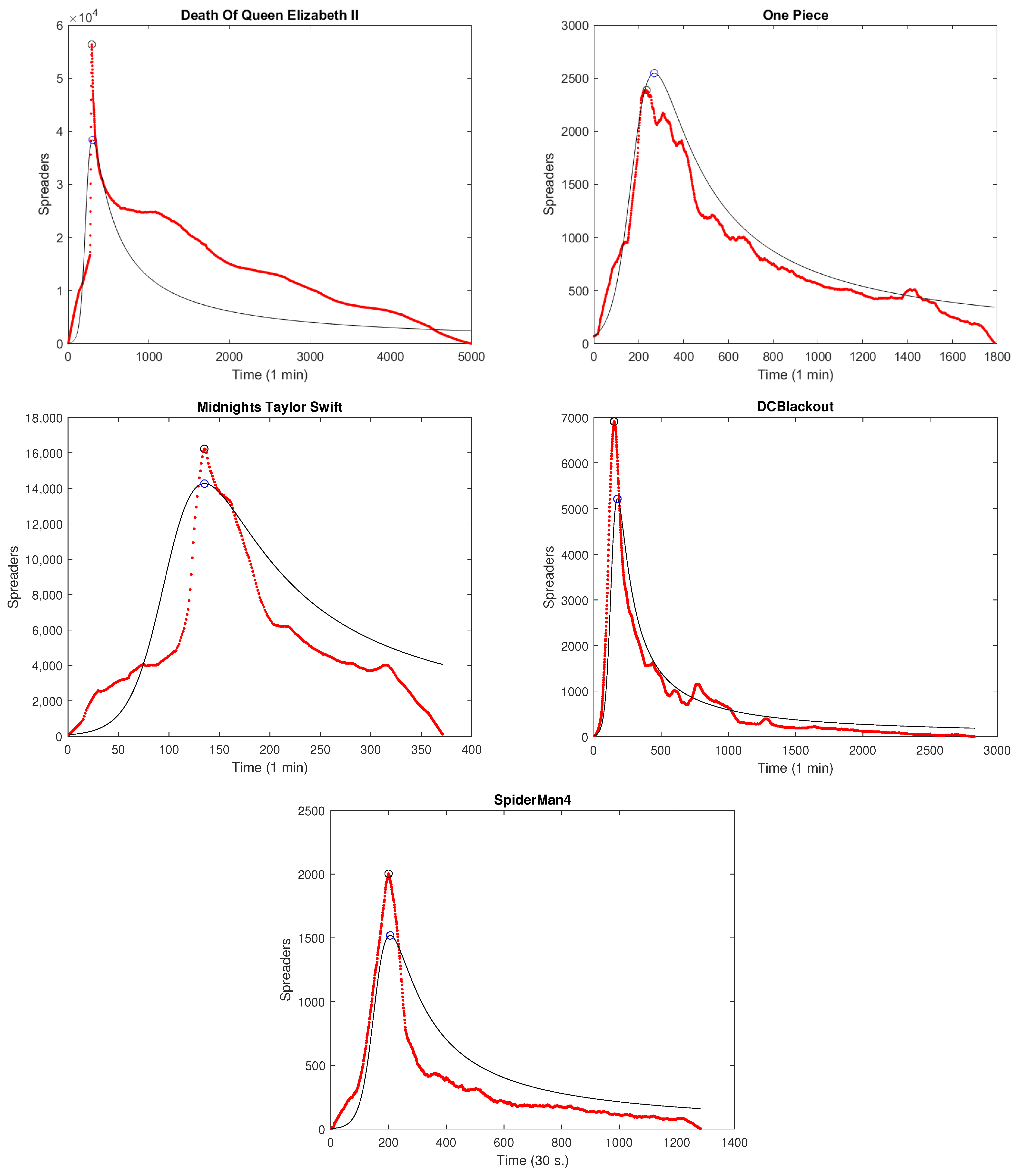
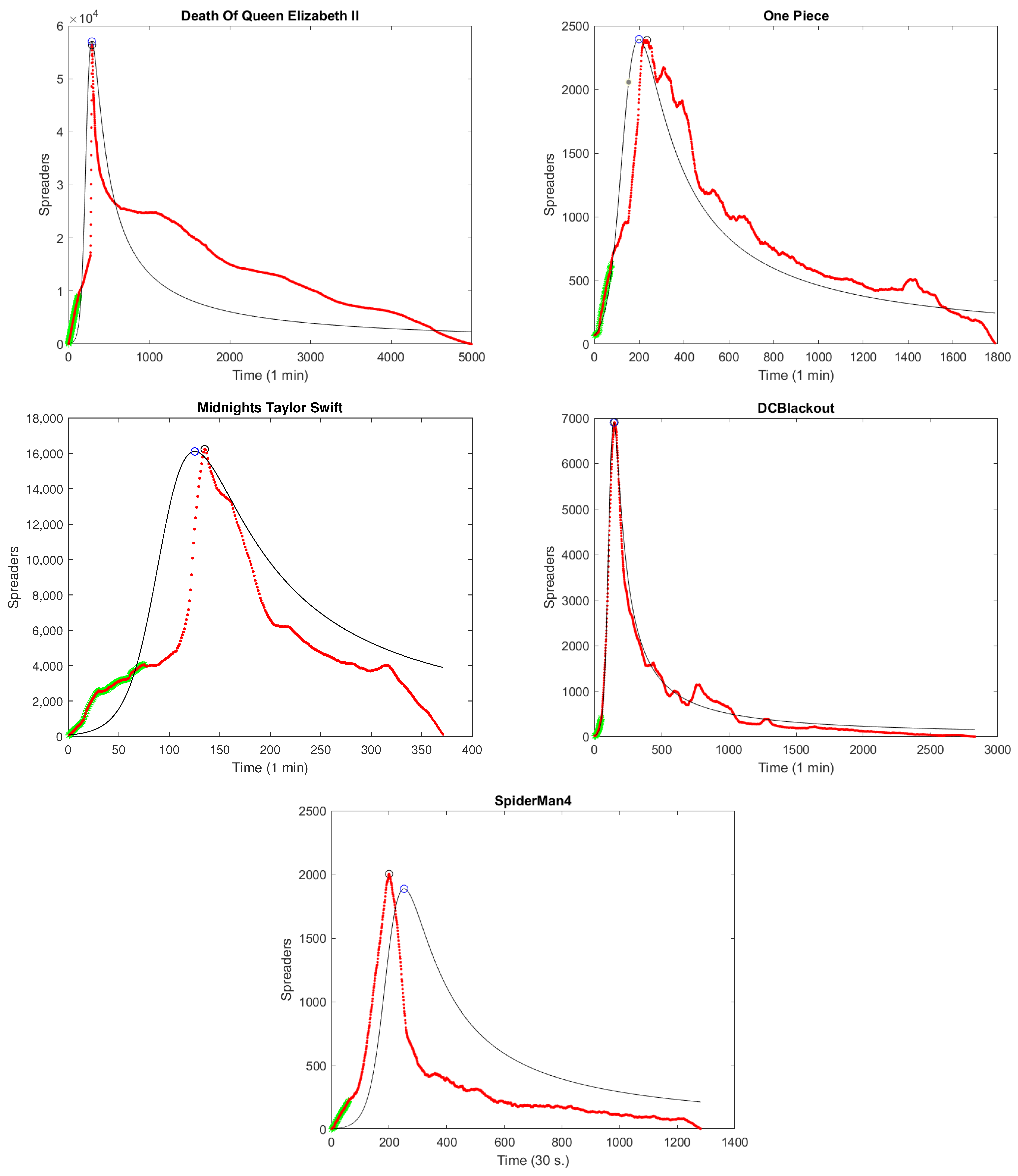
• The death of the Queen of the United Kingdom and other Commonwealth realms, Elizabeth II;
• The release of chapter number 1000 of the famous Japanese manga One Piece;
• The release of singer Taylor Swift’s new album, Midnights;
• The DCBlackout [10] rumor, which is related to an interruption of communication in Washington, D.C., due to Black Lives Matter Movement manifestations;
• The rumor related to the release of the movie Spiderman 4 on 3 May 2024 with the participation of the leading actor in other Spiderman movies from 2002 and 2007, Tobey Maguire. The rumor was spread by a user who used the name “Tobey Maguire” as his Twitter name and the same profile photo as the actor.

Some details about the data extracted from Twitter corresponding to the selected case studies are summarized in the following table (

Table 1. Details of the dataset.

Event	Date (d-m-y)	Duration	Scraped Tweets	Type	Hashtags
Death of Queen Elizabeth II	8 September 2022	2 days	485,011	News	#queenelizabeth, #queenelizabethII, #RIPqueenelizabeth, #RIPqueenelizabethII, #godsavethequeen
One Piece	1 March 2021	2 days	16,537	News	#onepiece
Taylor Swift’s Midnights	21 October 2022	6 h	106,716	News	#MidnightsTaylorSwift
DCBlackout	1 June 2020	2 days	33,117	Rumor	#DCBlackout
SpiderMan4	4 November 2022	10 h	7341	Rumor	#spiderman4

):

3.2. Parameter Estimation

The news items presented in Section 3.1 are various in terms of type (i.e., if they are true or rumors), number of data points collected, duration of diffusion and topic (we included news regarding politics, music and movies), and it is not easy to estimate parameters that fit real data in advance based only on these characteristics. Therefore, for each news item, a different set of estimated parameters was obtained. To this end, we employed the built-in lsqnonlin MATLAB function, which solves non-linear least squares problems. We used this function to find the set of parameters that minimizes a function; in this specific case, the function that computes the error between real data and approximated data. In particular, lsqnonlin allows users to choose between two different algorithms: the “Levenberg–Marquardt algorithm” and the “trust region reflective algorithm”. We used the second algorithm because it allows the user to choose an initial approximation, a lower bound and an upper bound for the vector of parameters that has to be optimized. In this way, it is possible to avoid the probabilities of some parameters becoming negative.

Hence, the proposed and implemented strategy consists of the following steps:

• Choice of a lower bound and an upper bound for the parameters to be optimized, i.e., $\beta$, $\gamma$ and k in the (1), and, possibly, the starting number of individuals belonging to each class ($I_0$, $S_0$ and $R_0$);
• Choice of a random initial approximation (inside the interval identified by the lower and upper bounds) for the set of parameters to be optimized;
• Computation of the function to be minimized, which measures the error between the real data and the data computed by solving system (1) ($OD{E}_S$) with the built-in ode45 MATLAB function. This error is computed by considering the entire dataset of real data or a part of it (built as Algorithm 1) and the solution of the $OD{E}_S$ system computed using parameters previously described. Therefore, if I, S and R are the vectors of real data so that $I_j$, $S_j$ and $R_j$ are the real numbers of ignorants, spreaders and recovered individuals at time $t_j$, respectively, and $I\left(t_j\right)$, $S\left(t_j\right)$ and $R\left(t_j\right)$ are the corresponding data computed by solving system (1), we compute the function to be minimized using the following formula:

  $$f(\beta ,\gamma ,\kappa )=\sum _{j=1}^n{(I_j-I\left(t_j\right))}^2+\sum _{j=1}^n{(S_j-S\left(t_j\right))}^2+\sum _{j=1}^n{(R_j-R\left(t_j\right))}^2$$

  where n is the total number of data points taken into consideration;
• Minimization of the obtained error by means of the built-in lsqnonlin MATLAB function and gain of the optimized parameters;
• Use of the optimized parameters to solve the ODEs system (1) in order to obtain a good approximation of the real data.

4. Results and Discussion

In this section, we provide a numerical demonstration of the proposed strategy, showing that using the right model and a good parameter estimation method, it is possible to both rebuild the evolution of news spread on a social network and to predict the evolution of this spread, even using few data points. Moreover, we underline the importance of accurate prediction of the peak of maximum diffusion of a news item, confirming our arguments. The model used for all numerical tests is the ISR model, as described in (1).

First, we analyze the diffusion of a news item using the entire dataset for parameters estimation. In this case, we minimize the error of all data in order to obtain the set of optimized values for the parameters $\beta ,\gamma$ and $\kappa$. The results are shown in Figure 4, where we show both real data obtained from Twitter using red markers and the curve obtained by solving the $OD{E}_s$ system using a black line. Also note that the x-axis label shown in parentheses is the time unit used for data collection.

In

Table 2. Results of peak estimation.

Event	${\mathit{t}}_{\mathit{exit}}$	${\mathit{t}}_{\mathit{p}}$	Estimated ${\mathit{t}}_{\mathit{p}}$	Relative Error
Death of Queen Elizabeth II	15 min	292	302.63	0.0364
One Piece	2 min	235	269.59	0.1472
Taylor Swift’s Midnights	15 min	135	135.16	0.0012
DCBlackout	60 min	150	175.09	0.1672
SpiderMan4	30 s	200	205.49	0.0275

, we report different parameters for each news item. First of all, we report the interval of time ($t_{exit}$) that, as explained in Section 3, we consider as the exit time from the “spreader” class to the “recovered” class if an user does not publish any other tweets containing the news item. Then, we report the time ($t_p$) when the peak of the spread occurs, considering both the real peak and the estimated peak. Finally, we report the relative error in the computation of the peak, which allows us to measure how accurate the prediction is.

Considering these results, we can say that using all data, we were able to achieve an approximation of the diffusion of the news that is sufficiently accurate, particularly if we consider the time of the peak of the diffusion. However, in some cases, for example, the case of the news regarding the death of Queen Elizabeth II or the rumor spread with hashtag #DCBlackout, we were able to accurately predict the time of the peak but with a underestimation of size of the spreader class at that time.

Moreover, there is another aspect that is necessary to take into consideration. In real life, the peak of the diffusion of news occurs in a relatively short period of time. For examples, for the news regarding the death of Queen Elizabeth II, the real peak occurs at time 292 (of the graphic). This means that it happens 292 min (approximately 5 h) after the beginning of observation of the event. Similarly, for the rumor spread with hashtag #spiderman4, the peak occurs after 100 min (approximately after an hour and an half). This means that if we want to know the peak of a news item in advance, before it happens in reality, we have to observe the event only for a short period of time to be able to predict its evolution starting from the limited data available at the moment of observation. For this reason, in the following part of this section, we show the results obtained considering only a part of the dataset. In our tests, we used as few data points as possible in order to minimize the error between real data and computed data, obtaining a set of optimized parameters, while the rest of the dataset was used to prove that the prediction made with the obtained parameters was still correct. Moreover, unlike the previous case, when we used all of the dataset, we decided to include the initial number of ignorants and spreaders in the optimization process, while the initial number of recovered class members was set to 0 in all cases because at the beginning, there is nothing to recover from. The prediction on the number of spreaders is shown in Figure 5, with green markers underlining data used for the fitting phase and red markers representing data used to validate the model.

As we can see from Figure 5, using fewer data, we also achieved an accurate result, which, in some cases, is also better than the results obtained with more data shown in Figure 4 in terms of estimation of the time of the peak ($t_p$) and the number of spreaders at the peak. This may be explained by the fact that minimizing the error between real data and output data, we aimed to produce the best fit during the entire period of study. However, in this way, the error of the final data affects the parameter estimation so much that the estimated peak of the maximum spread is negatively affected. An example can be made considering the trend of the news related to Queen Elizabeth’s death or considering the trend of the two rumors. Using all data for the fitting phase, we obtained an underestimation of the number of spreaders at the time of the peak, whereas using fewer data and focusing only on the beginning of the information spread, we obtained a good estimation of the values for the peak, both in terms of time and the number of total spreaders.

In particular,

Table 3. Results for the peak estimation using fewer data.

Event	${\mathit{t}}_{\mathit{fit}}$	${\mathit{t}}_{\mathit{p}}$	Estimated ${\mathit{t}}_{\mathit{p}}$	Relative Error
Death of Queen Elizabeth II	124	292	289.00	0.0103
One Piece	75	235	199.06	0.1530
Taylor Swift’s Midnights	75	135	125.13	0.0731
DCBlackout	52	150	143.54	0.0431
SpiderMan4	59	200	252.22	0.2611

shows the results obtained for peak estimation and the corresponding obtained error, using the values reported in Table 1 as values for the duration period and the same values shown in Table 2 for the values of $t_{exit}$ of each news item. The time ($t_{fit}$) in Table 3 represents the time interval corresponding to the data used for the estimation of parameters.

We can also make a comparison between the results obtained in the case of the fitting phase performed using the entire dataset and the results obtained with the fitting phase performed using fewer data and the number of initial ignorants and spreaders optimized. The results are shown in the following tables (

Table 4. Values of model parameters for the first strategy (all data used for the fitting phase).

Event	$\mathit{\beta }$	$\mathit{\gamma }$	$\mathit{\kappa }$
Death of Queen Elizabeth II	0.153463878328834	1.02393738655116	0.195770170416092
One Piece	0.198124671775847	0.532629600626445	0.113619513008026
Taylor Swift’s Midnights	0.444216647629681	0.823325900401598	0.125904515289138
DCBlackout	0.127744561954384	0.286654749230175	0.358841966601127
SpiderMan4	0.410490456996288	1.106571906515240	0.100000063575436

,

Table 5. Valuesof model parameters for second strategy (fewer data used for the fitting phase).

Event	$\mathit{\beta }$	$\mathit{\gamma }$	$\mathit{\kappa }$
Death of Queen Elizabeth II	0.541078205848684	2.12886024675943	0.0592169183830037
One Piece	0.0919624956640816	0.271256024892648	0.32997392156807
Taylor Swift’s Midnights	0.119443419484832	0.17979093995445	0.512263317095459
DCBlackout	0.0469306748441707	0.0657201832547797	1.22327435650595
SpiderMan4	0.041648371956623	0.07954719564129	0.815615022612782

and

Table 6. Totalnumber of spreaders using the first strategy (all data used for the fitting phase).

Event	Maximum Spreader Value	Approximated Maximum Spreader Value	Relative Error
Death of Queen Elizabeth II	56,344	38,387.0	0.3187
One Piece	2387	2547.2	0.0671
Taylor Swift’s Midnights	16,230	14,266.0	0.1210
DCBlackout	6907	5214.5	0.2450
SpiderMan4	2003	1517.2	0.2425

), reporting the values of model parameters using the entire dataset for the fitting phase or fewer data. The results of the prediction of the maximum number of spreaders using all data and the results of the maximum number of spreaders using fewer data are also reported.

In the following table (

Table 7. Totalnumber of spreaders using the second strategy (fewer data used for the fitting phase).

Event	Initial Ignorants	Initial Spreaders	Maximum Spreader Value	Approximated Maximum Spreader Value	Relative Error
Death of Queen Elizabeth II	51,403	1191	56,344	57,038.0	0.0123
One Piece	10,000	95	2387	2394.4	0.0031
Taylor Swift’s Midnights	11,264	654	16,230	16,112.0	0.0073
DCBlackout	10,000	26	6907	6900.7	0.0009
SpiderMan4	10,000	36	2003	1887.3	0.0578

), due to the fact that we also optimized the number of initial ignorants and spreaders, these optimized values are inserted.

As we can see, the difference in the obtained values is not considerable, although it may be significant if we really want to predict the trend of a news item with few available data points.

Moreover, parameter estimation is more accurate with more available tweets. Obviously, tweets can be downloaded only from non-private Twitter accounts, so this means that the kind of news is relevant because the number of available tweets is higher for international news than for news or rumors that spread locally.

At the same time, this factor underlines that our strategy to predict trends of news or rumors, emphasizing the importance of good computation of the peak of the maximum spread and not only the entire evolution of the trend during the course of time, is efficient and truly applicable. This is even more evident if we consider that in real life, we will probably not have the time to study a news item for a long period of time, waiting for the acquisition of more data before it happens. Moreover, some improvements could be achieved in terms of the kind of model used for predictions. As shown in [36], a better prediction of the peak of the number of spreaders could be obtained by raising the order of the differential equation system.

5. Conclusions

In this work, we analyzed the use of the ISR model to study the spread of information on Twitter. We tested it on real news and rumor data, developing and showing the results of two different strategies to study their trends. The first strategy uses the entire dataset to fit data and obtain optimized parameters, and the second strategy uses fewer data and is recommended to estimate the time of the maximum spread. This second approach is the main novelty of our work; it is useful not only from an academic point of view. In real life, if we want to study the spread of a real news item, it is impossible to observe its evolution for a long period of time. Generally, we need to analyze it as fast as possible because in this way, as underlined, we are able to use our predictions for practical aims, such as the development of software enabling us to block a rumor and to provide a tool that can be integrated into the algorithm of the social network or the development of successful marketing strategies. Certainly, this second strategy could be improved, in particular as concerns the peak of the number of spreaders. Different approaches could be used, for example, the raising of the order of the differential equation system. Moreover, it could be also interesting to propose a mathematical formula to calculate some parameters, such as the aforementioned ($t_{exit}$), that are fundamental during the dataset construction process. All these suggestions could become the main aims of future research works.

References

1. Rastogi, S.; Bansal, D. A review on fake news detection 3T’s: Typology, time of detection, taxonomies. Int. J. Inf. Secur. 2023, 22, 177–212. [Google Scholar] [CrossRef] [PubMed]
2. The Ji Village News Mathematical Modelling of Fake-News. Available online: https://www.haidongji.com/2018/07/23/mathematical-modeling-of-fake-news/ (accessed on 23 March 2022).
3. Abdullah, S.; Wu, X. An epidemic model for news spreading on Twitter. In Proceedings of the 23rd IEEE International Conference on Tools with Artificial Intelligence, ICTAI, Boca Raton, FL, USA, 7–9 November 2011; Volume 2011, pp. 163–169. [Google Scholar]
4. Cardone, A.; Díaz de Alba, P.; Paternoster, B. Influence of age group in the spreading of fake news: Contact matrices in social media. In Proceedings of the IEEE 16th International Conference on Signal Image Technology& and Internet Based Systems (SITIS), Dijon, France, 19–21 October 2022; pp. 515–521. [Google Scholar]
5. D’Ambrosio, R.; Díaz de Alba, P.; Giordano, G.; Paternoster, B. A modified SEIR model: Stiffness analysis and application to the diffusion of fake news. In Computational Science and Its Applications, Proceedings of the 22nd International Conference, Malaga, Spain, 4–7 July 2022, Proceedings, Part I; Gervasi, O., Murgante, B., Hendrix, E.M.T., Taniar, D., Apduhan, B.O., Eds.; Springer: Cham, Switzerland, 2022; Volume 13375, pp. 90–103. [Google Scholar]
6. D’Ambrosio, R.; Giordano, G.; Mottola, S.; Paternoster, B. Stiffness analysis to predict the spread out of fake information. Future Internet 2021, 13, 222. [Google Scholar] [CrossRef]
7. Din, R.; Algehyne, E.A. Mathematical analysis of COVID-19 by using SIR model with convex incidence rate. Results Phys. 2021, 23, 103970. [Google Scholar] [CrossRef] [PubMed]
8. He, H.; Peng, Y.; Sun, K. SEIR modeling of the COVID-19 and its dynamics. Nonlinear Dyn. 2020, 101, 1667–1680. [Google Scholar] [CrossRef]
9. Lacitignola, D.; Diele, F. Using awareness to Z-control a SEIR model with overexposure: Insights on COVID-19 pandemic. Chaos Solit. 2021, 150, 111063. [Google Scholar] [CrossRef]
10. Maleki, M.; Mead, E.; Arani, M.; Agarwal, N. Using an epidemiological model to study the spread of misinformation during the Black Lives Matter Movement. arXiv 2021, arXiv:2103.12191. [Google Scholar]
11. Muhlmeyer, M.; Agarwal, S. Information spread in a social media age. In Modelling and Control; CRC Press: Boca Raton, FL, USA; Taylor and Francis Group: Boca Raton, FL, USA; London, UK; New York, NY, USA, 2021. [Google Scholar]
12. Muhlmeyer, M.; Agarwal, S.; Huang, A. Modeling social contagion and information diffusion in complex socio-technical systems. IEEE Syst. J. 2020, 14, 5187–5198. [Google Scholar] [CrossRef]
13. Muhlmeyer, M.; Huang, J.; Agarwal, S. Event Triggered Social Media Chatter: A New Modeling Framework. IEEE Trans. Comput. Soc. Syst. 2019, 6, 197–207. [Google Scholar] [CrossRef]
14. Kevrekidis, P.G.; Cuevas-Maraver, J.; Drossinos, Y.; Rapti, Z.; Kevrekidis, G.A. Reaction-diffusion spatial modeling of COVID-19: Greece and Andalusia as case examples. Phys. Rev. E 2021, 104, 024412. [Google Scholar] [CrossRef]
15. Martin, O.; Fernandez-Diclo, Y.; Coville, J.; Soubeyrand, S. Equilibrium and sensitivity analysis of a spatio-temporal host-vector epidemic model. Nonlinear Anal. Real World Appl. 2021, 57, 103194. [Google Scholar] [CrossRef]
16. Song, P.; Xiao, Y. Analysis of a diffusive epidemic system with spatial heterogeneity and lag effect of media impact. J. Math. Biol. 2022, 85, 17. [Google Scholar] [CrossRef] [PubMed]
17. Wang, H.; Wang, F.; Xu, K. Modeling Information Diffusion in Online Social Networks with Partial Differential Equations; Springer: Cham, Switzerland, 2020; Volume 7. [Google Scholar]
18. Grave, M.; Viguerie, A.; Barros, G.F.; Reali, A.; Andrade Roberto, F.S.; Coutinho Alvaro, L.G.A. Modeling nonlocal behavior in epidemics via a reaction-diffusion system incorporating population movement along a network. Comput. Methods Appl. Mech. Engrg. 2022, 401, 115541. [Google Scholar] [CrossRef] [PubMed]
19. Hill, E.M. Modelling the epidemiological implications for SARS-CoV-2 of Christmas household bubbles in England. J. Theor. Biol. 2023, 557, 111331. [Google Scholar] [CrossRef] [PubMed]
20. Omame, A.; Abbas, M.; Din, A. Global asymptotic stability, extinction and ergodic stationary distribution in a stochastic model for dual variants of SARS-CoV-2. Math. Comput. Simul. 2023, 204, 302–336. [Google Scholar] [CrossRef]
21. Yang, J.; Shi, X.; Song, X.; Zhao, Z. Threshold dynamics of a stochastic SIQR epidemic model with imperfect quarantine. Appl. Math. Lett. 2023, 136, 108459. [Google Scholar] [CrossRef]
22. Martcheva, M. An Introduction to Mathematical Epidemiology; Springer: Cham, Switzerland, 2015; Volume 61. [Google Scholar]
23. Blanes, S.; Iserles, A.; Macnamara, S. Positivity-preserving methods for ordinary differential equations. ESAIM Math. Model. Numer. Anal. 2022, 56, 1843–1870. [Google Scholar] [CrossRef]
24. Conte, D.; Guarino, N.; Pagano, G.; Paternoster, B. On the Advantages of Nonstandard Finite Difference Discretizations for Differential Problems. Numer. Anal. Appl. 2022, 15, 219–235. [Google Scholar] [CrossRef]
25. Conte, D.; Guarino, N.; Pagano, G.; Paternoster, B. Positivity-preserving and elementary stable nonstandard method for a COVID-19 SIR model. Dolomites Res. Notes Approx. 2022, 15, 65–77. [Google Scholar]
26. Conte, D.; Pagano, G.; Paternoster, B. Nonstandard finite differences numerical methods for a vegetation reaction-diffusion model. J. Comput. Appl. Math. 2023, 419, 114790. [Google Scholar] [CrossRef]
27. Scalone, C. Positivity preserving stochastic θ-methods for selected SDEs. Appl. Numer. Math. 2022, 172, 351–358. [Google Scholar] [CrossRef]
28. Cardone, A.; D’Ambrosio, R.; Paternoster, B. Exponentially fitted IMEX methods for advection–diffusion problems. J. Comput. Appl. Math. 2017, 316, 100–108. [Google Scholar] [CrossRef]
29. Cardone, A.; Ixaru, L.G.; Paternoster, B.; Santomauro, G. Ef-Gaussian direct quadrature methods for Volterra integral equations with periodic solution. Math. Comput. Simul. 2014, 110, 125–143. [Google Scholar] [CrossRef]
30. D’Ambrosio, R.; Moccaldi, M.; Paternoster, B. Numerical preservation of long-term dynamics by stochastic two-step methods. Discret. Contin. Dyn. Syst. Ser. B. 2018, 23, 2763–2773. [Google Scholar] [CrossRef]
31. Frasca-Caccia, G.; Hydon, P.E. Numerical preservation of multiple local conservation laws. Appl. Math. Comput. 2021, 403, 126203. [Google Scholar] [CrossRef]
32. Frasca-Caccia, G.; Hydon, P.E. A New Technique for Preserving Conservation Laws. Found. Comput. Math. 2022, 22, 477–506. [Google Scholar] [CrossRef]
33. Ignatius, D. Modeling the Spread of Information on Twitter. Master’s Thesis, California State Polytechnic University, Pomona, CA, USA, 2018. [Google Scholar]
34. Twitter Developer Option. Available online: www.developer.twitter.com (accessed on 7 December 2022).
35. Tweepy Documentation. Available online: https://docs.tweepy.org/en/latest/ (accessed on 7 December 2022).
36. Koppelaar, H.; Nasehpour, P. Series Solution of High Order Abel, Bernoulli, Chini and Riccati Equations. Kyungpook Math. J. 2022, 62, 729–736. [Google Scholar]
Figure 1. Graph of the ISR model.
Algorithms 16 00391 g001
Figure 2. Graph of the IESZ model.
Algorithms 16 00391 g002
Figure 3. Time evolution of the ISR model and IESZ model with parameters (3) and (4), respectively.
Algorithms 16 00391 g003
Figure 4. Spreader prediction obtained using all data for parameter estimation. Red marker (∘): real number of spreaders. Black line: estimated number of spreaders. Blue marker (∘): maximum number of estimated spreaders. Black marker (∘): maximum number of real spreaders.
Algorithms 16 00391 g004
Figure 5. Spreader prediction obtained using fewer data for parameter estimation. Green marker (*): data used for the fitting phase. Red marker (∘): data used for model validation. Black line: estimated number of spreaders. Blue marker (∘): maximum number of estimated spreaders. Black marker (∘): maximum number of real spreaders.
Algorithms 16 00391 g005