Vector Control of PMSM Using TD3 Reinforcement Learning Algorithm

Abstract

Permanent magnet synchronous motor (PMSM) drive systems are commonly utilized in mobile electric drive systems due to their high efficiency, high power density, and low maintenance cost. To reduce the tracking error of the permanent magnet synchronous motor, a reinforcement learning (RL) control algorithm based on double delay deterministic gradient algorithm (TD3) is proposed. The physical modeling of PMSM is carried out in Simulink, and the current controller controlling i_d-axis and i_q-axis in the current loop is replaced by a reinforcement learning controller. The optimal control network parameters were obtained through simulation learning, and DDPG, BP, and LQG algorithms were simulated and compared under the same conditions. In the experiment part, the trained RL network was compiled into C code according to the workflow with the help of rapid prototyping control, and then downloaded to the controller for testing. The measured output signal is consistent with the simulation results, which shows that the algorithm can significantly reduce the tracking error under the variable speed of the motor, making the system have a fast response.

1. Introduction

Due to their simple form, high power density, and high efficiency, PMSMs are widely employed in numerous industrial control applications [1,2,3]. The speed of PMSM is mainly regulated by frequency conversion. Closed-loop speed constant voltage frequency ratio control (V/F), vector control (VC), and direct torque control are widely used in frequency conversion speed control [4]. The most common is VC, also known as magnetic Field-Oriented Control (FOC), which uses a variable-frequency drive (VFD) control three-phase alternating current (AC) motor to control the output of the motor by adjusting the frequency converter’s output frequency, output voltage size, and angle [5]. In this paper, the i_d-axis and i_q-axis of the current loop are accurately controlled by reinforcement learning method under the FOC framework, so that the inverter can output a suitable PWM signal and obtain accurate motor speed, providing a new current loop control method.

PMSM is a complex object with multiple variables, strong coupling, and nonlinear and variable parameters. To obtain better control performance, many scholars have designed a reasonable controller [6]. Chang, X. et al. [7] proposed a non-singular fast terminal sliding mode (NNFTSM) control strategy based on extended state observer (ESO) and tracking differential (TD), in which PMSM has strong robustness to parameter changes and external load disturbances. Chen, J. et al. [8] adopted a nonlinear adaptive control (NAC) method of PMSM to estimate the concentrated disturbance terms through the observer, thus achieving better dynamic performance of the system. Dai, C. et al. [9] proposed a current restraint controller based on interference observer for PMSM speed control to reduce the interference of current constraints and external conditions. Guo, T. et al. [10] constructed a special nonlinear gain to directly establish the Q-axis current penalty mechanism in the PMSM control action, which solves the problem of overcurrent protection under fast dynamic conditions. With the rapid development of computer technology, many scholars have done more research on the intelligent control of PMSM. Xu, Q. et al. [11] adopted NSGA-II (Non-dominated Sorting Genetic Algorithm-II) to optimize the PID controller parameters of PMSM. Zhang, W. et al. [12] proposed a new energy efficiency-oriented sliding mode controller (APIDSMC-PALC) compensation method to suppress the influence of PMSM servo system torque ripple.

Deep reinforcement learning (DRL) is an ideal multi-objective optimization method with a high searching ability and a quick convergence rate, and it has demonstrated high application value in the control sector in recent years. Lu, W. et al. [13] made a control autonomous underwater vehicle (AUV) by model-free RL based on data informed domain randomization (DDR) that enables the controller to adapt to sudden changes in dynamics. Zhang, L. et al. [14] used the RL framework with Actor-Critic network as a new path ordering algorithm (PRA) to carry out effective relationship learning and path finding, reducing the dependence on large-scale training data sets. Zhao, B. et al. [15] integrated input and output data and cyclic neural networks, established an observer to approximate unknown system dynamics, and solved the problem of optimal stability of unknown nonlinear systems affected by uncertain input constraints. Zhang, S. et al. [16] used DRL to enable unmanned aerial vehicles (UAVs) to perform navigation tasks randomly and dynamically in a multi-obstacle environment. Hong, Z. et al. [17] proposed a control method of reinforcement learning-PI based on genetic algorithm. The model was built, and the initial parameters of PI controller were optimized by genetic algorithm. The depth deterministic strategy gradient algorithm was used to adjust the PI controller in real time, which realizes the function of position command control of the air rudder servo system. Yang, C. et al. [18] view of the uncertainty of model parameters and the dynamic coexistence of fast and slow, a reinforcement learning algorithm independent of model parameters is proposed to learn controller gain. This method improved the tracking performance and synchronization performance of the dual-motor system, inhibited the interference of unknown time-varying load, and avoided the influence of parameter uncertainty. With the wide application of intelligent control, in motor control, the operation of the motor includes uncertain factors such as the parameter change and operation disturbance of the motor. The influence of parameter changes and nonlinear interference in the motor system can be overcome through reinforcement learning training. The powerful self-learning ability of RL can be used to improve the control strategy of the system through data, and the optimal control of the motor can be realized.

In this paper, a current loop controller of PMSM based on RL is studied. PI controller in FOC current loop is replaced by RL controller, RL training environment is constructed, and TD3-RL decision mechanism is introduced to train parameters in Actor and Critic network offline until the expected current control effect is achieved. Finally, a rapid prototype test was designed, and the RL controller was compiled into C code and downloaded into the controller for testing, which verified the speed and effectiveness of the TD3-FOC controller in the speed control of PMSM.

2. PMSM Model and RL

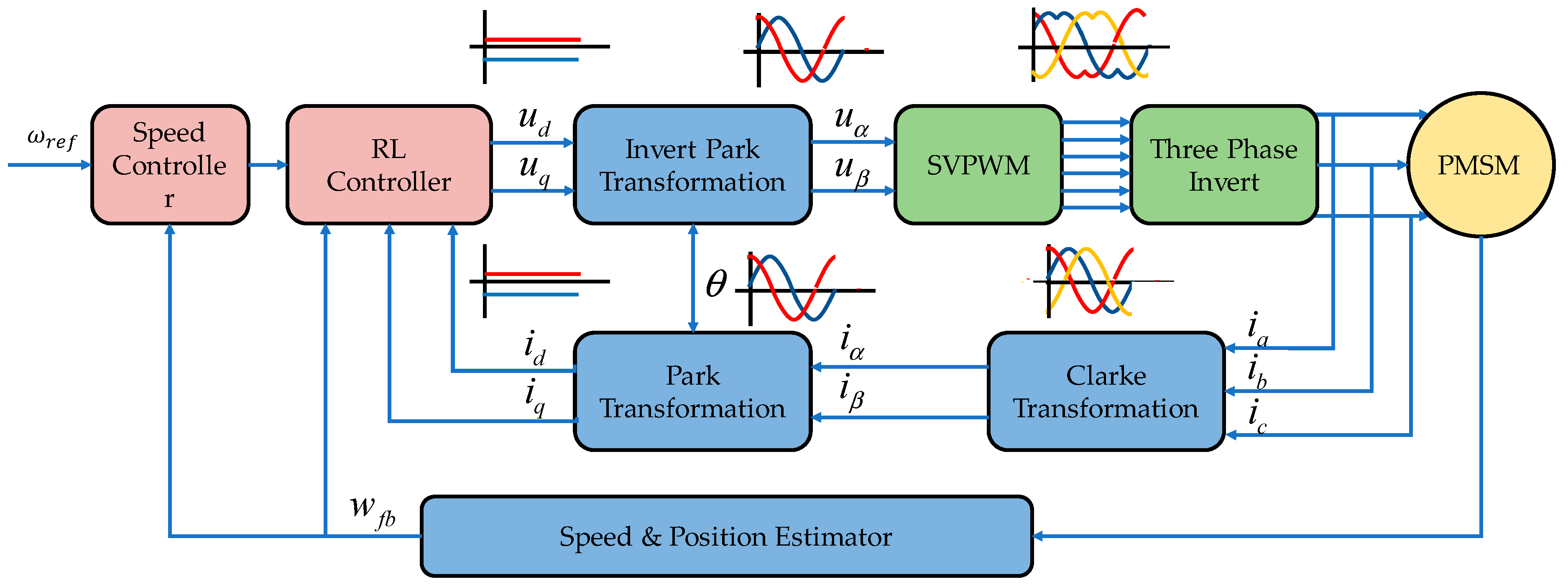
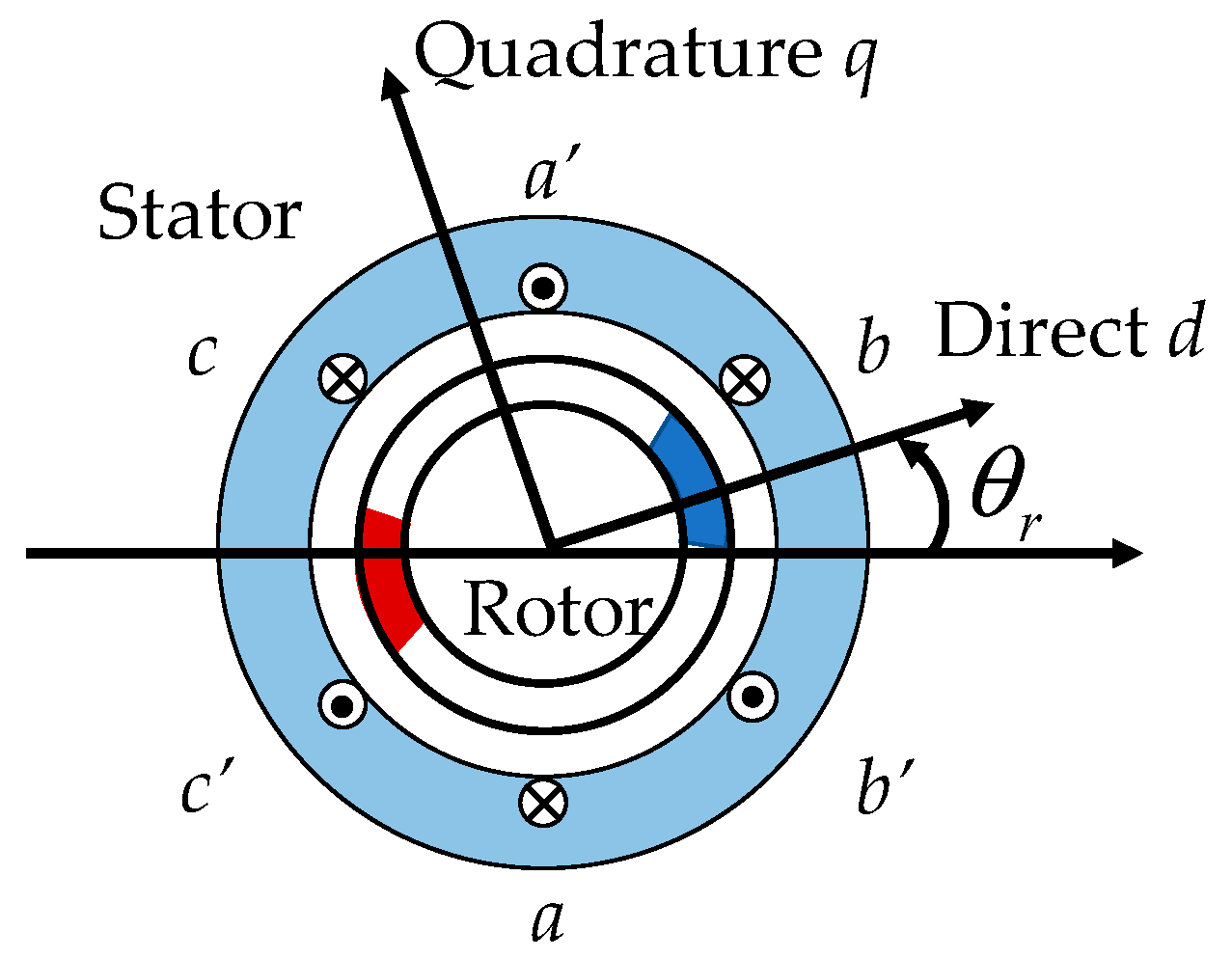
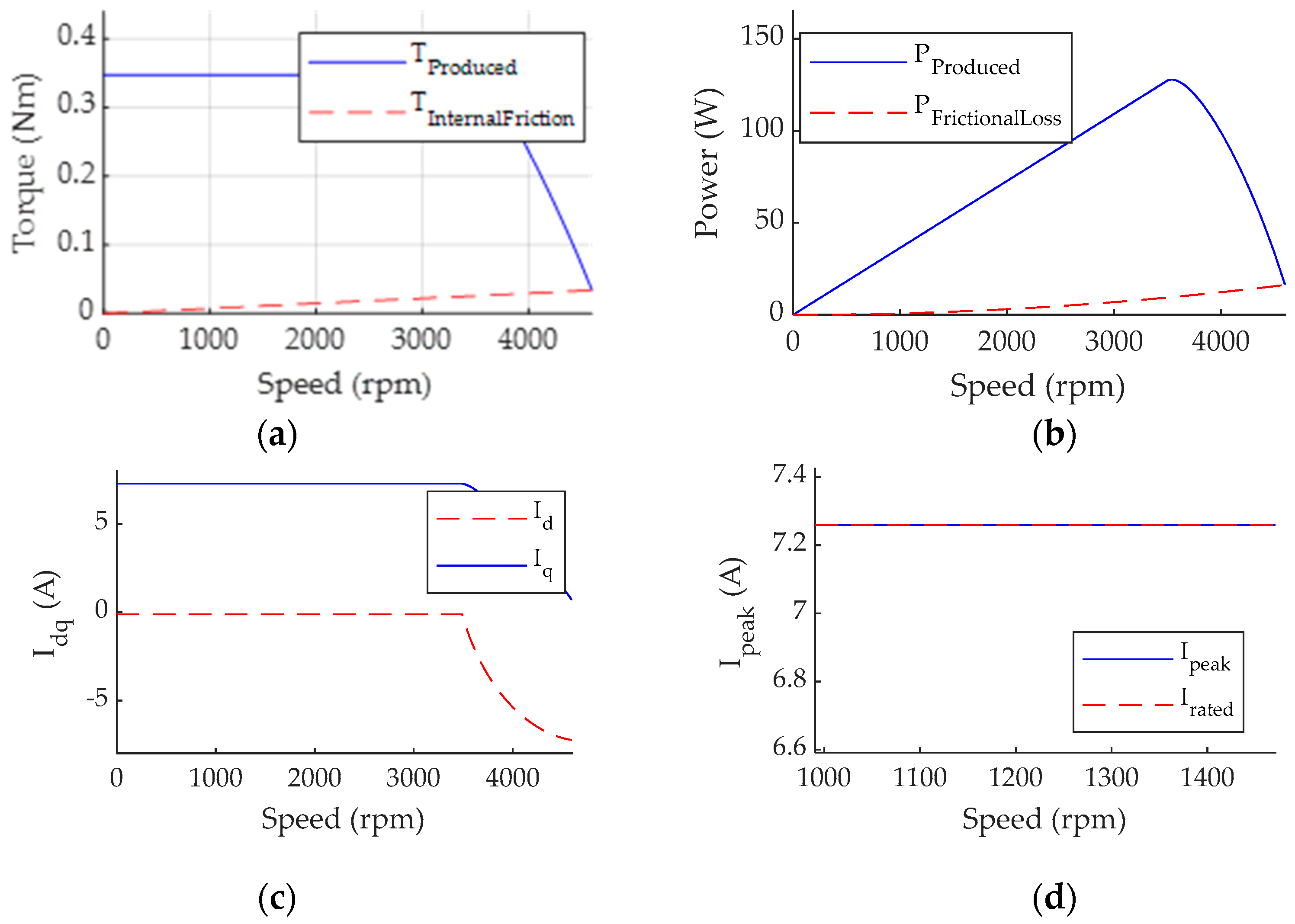
2.1. PMSM Model

The essential components of a PMSM are a permanent magnet pole rotor and a three-phase winding fixed stator. A rotating magnetic field is produced when a three-phase AC power supply is applied to the stator winding [19]. The magnetic poles on the rotor interact with the revolving magnetic field to produce an electromagnetic torque that excites the rotor to rotate synchronously. The principle of PMSM is shown in Figure 1.

$$\begin{array}{l}{u}_d=R_s{i}_d+L_d\frac{d_{i_d}}{dt}-\omega L_q{i}_q\\ u_q=R_s{i}_q+L_q\frac{d_{i_q}}{dt}+\omega (L_d{i}_d+{\varphi }_f)\end{array}\}$$

(1)

where u_d—D-axis voltage; u_q—Q-axis voltage; R_s—stator resistance; i_d—D-axis current; i_q—Q-axis current; L_d—D-axis equivalent inductance; L_q—Q-axis equivalent inductance; ω—rotor angular velocity; ϕ_f—Number of flux linkage.

Figure 1. PMSM rotation schematic.

The principle of vector control of PMSM servo system, when i_d is equal to 0, the D-axis voltage u_d is transformed into:

$$u_d=-\omega L_q{i}_q.$$

(2)

When the D-axis current reaches zero, the D-axis current no longer contributes to the torque voltage. Electromagnetic torque is generated by the current of the motor. We can change the torque of the motor by changing the Q-axis current i_q. To map the change in force, the frequency of the current can also be adjusted to control the speed. Finally, the duration of the speed is used to control the motor speed.

This paper uses RL controller to control the current of PMSM current loop. A typical FOC architecture was developed in Simulink, where the outer loop controller controls the speed, while the inner loop PI controller controls the D-axis and Q-axis currents (Figure 2). The RL module is created in the current loop, which replaces the current loop PI controller for this architecture.

Figure 2. RL-FOC for PMSM.

The whole FOC control system consists of three parts, PMSM model, inverter model, and reinforcement learning model, in which the FOC control framework has two control loops: the external loop uses PI controller to change the speed, and the internal loop uses RL agent to change the D-axis and Q-axis current.

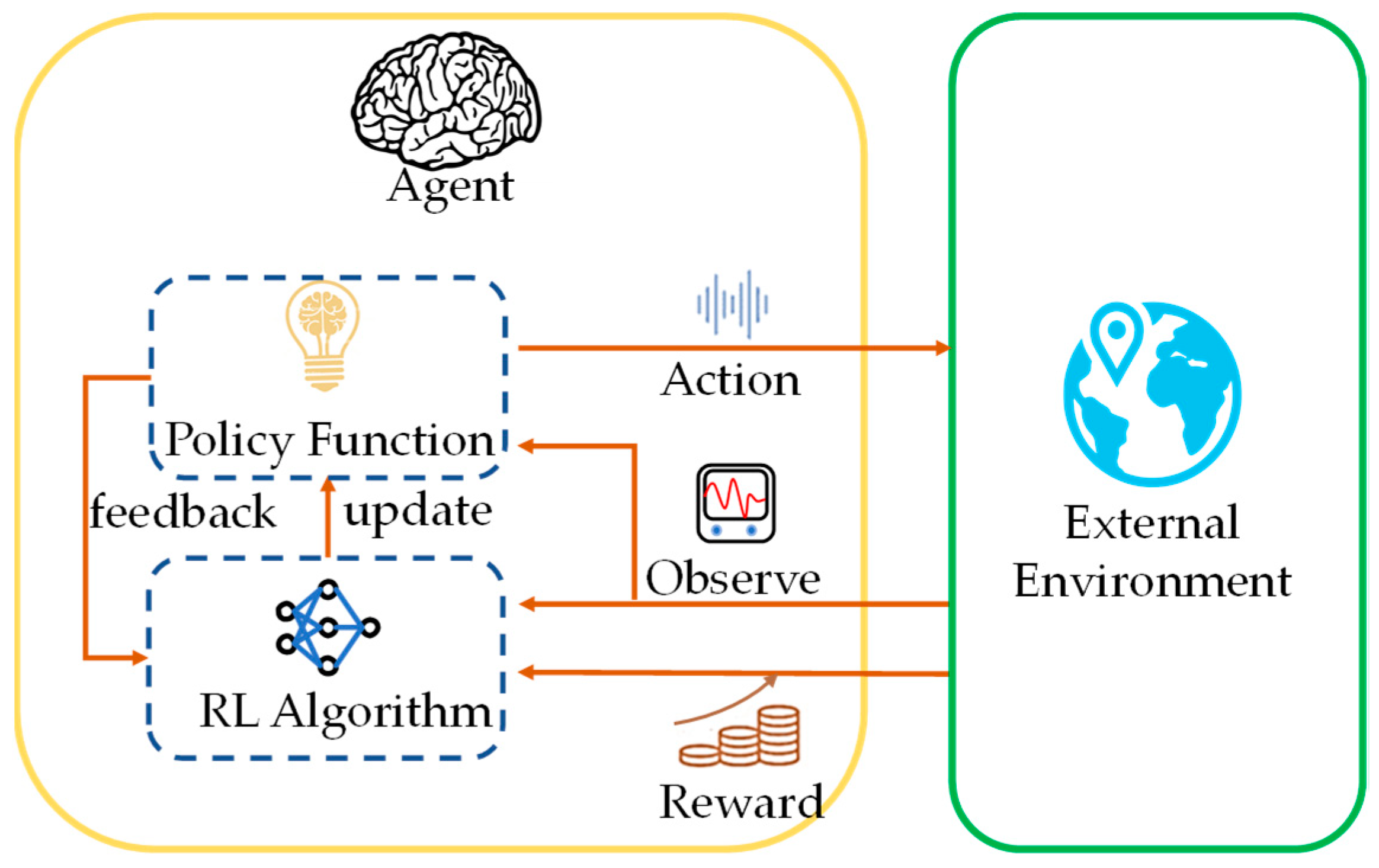
2.2. Reinforcement Learning

Reinforcement Learning (RL), also known as evaluation learning, is one of the paradigms and methodologies of machine learning, which is used to describe and solve the problem that agents use learning strategies to maximize returns or achieve specific goals in the interaction process with the environment, the agent is a self-iterative network integration module. RL is a learning mechanism for learning how to map from state to behavior to maximize the reward obtained [20].

The architecture of RL can be represented by the following Figure 3. The brain refers to the agent and the earth refers to the external environment. Starting from the current state S, after action a is taken, the action gets the corresponding reward value for the current environment. It feeds back the reward signal R (which represents how good or bad behavior A is for the final goal) to the agent, so the agent can form a loop, observe some information from the loop, enter a new state S’, and then make new behaviors and keep repeating this process until the goal is achieved. The basic process of RL follows such an architecture [21,22,23].

Figure 3. The basic framework of RL.

In contrast to traditional control methods (Figure 4), reinforcement learning is the act of observing the environment and performing the task in an optimal way, a process that is equivalent to a controller in a control system. Table 1 can be used to map the RL components to the control system [24,25,26].

Figure 4. Conventional control methods.

Table 1. RL and traditional control scheme architecture mapping table.

RL	Control System
Policy	Controller
Environment	Everything except the controller—The environment in the figure above contains the plant, the reference signal, and the estimated error value.
Observation	Any quantifiable value visible to the agent from the environment
Action	Regulate or alter variables
Reward	A measurement, an error signal, or a function of another performance metric
Learning algorithm	Adaptive mechanism

Traditional control is based on feedback control and state-based modeling control. Reinforcement learning control started late, and optimal control and reinforcement learning were not integrated until the Bellman equation in the 1960s. Then, scholars have proposed various model-based and model-free reinforcement learning methods, and RL is currently used significantly in trajectory planning and motion control. RL algorithms (such as DQN, A2C, Actor-Critic, and others) offer a variety of methods for updating training strategies, and these training algorithms are mostly used to make decisions for complex systems such as robots and cars [27,28,29].

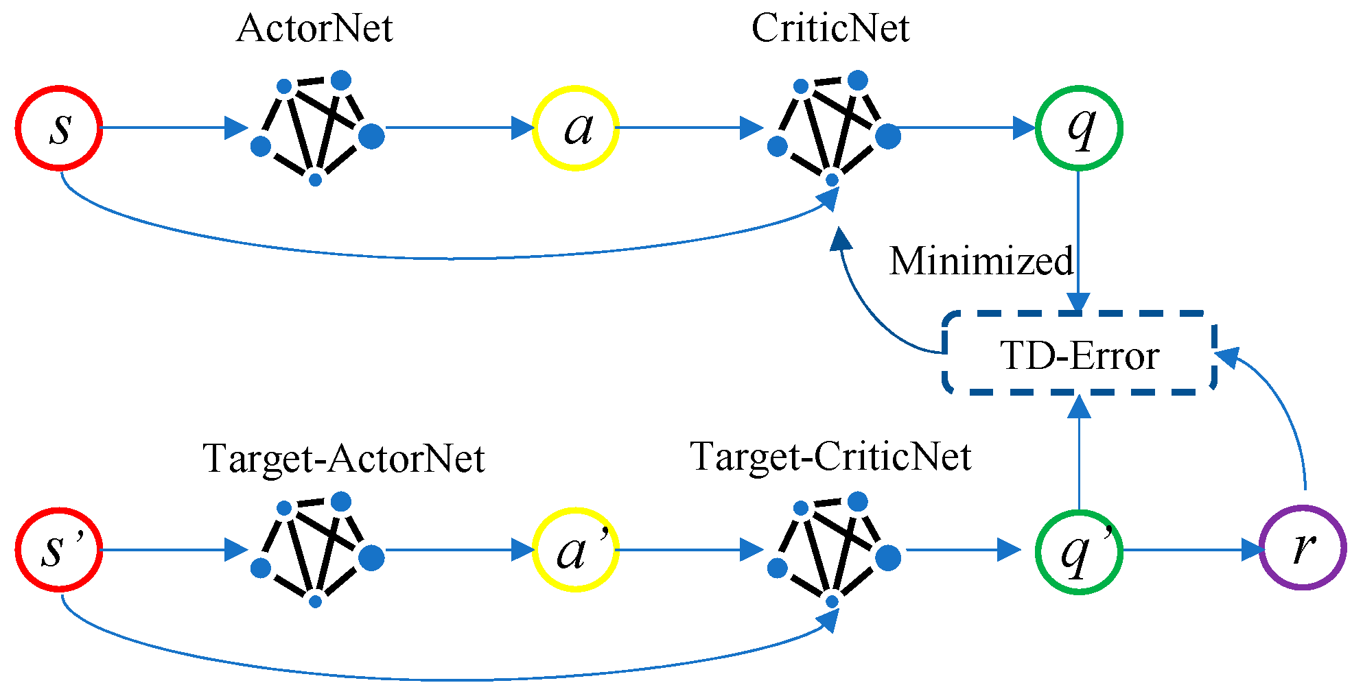
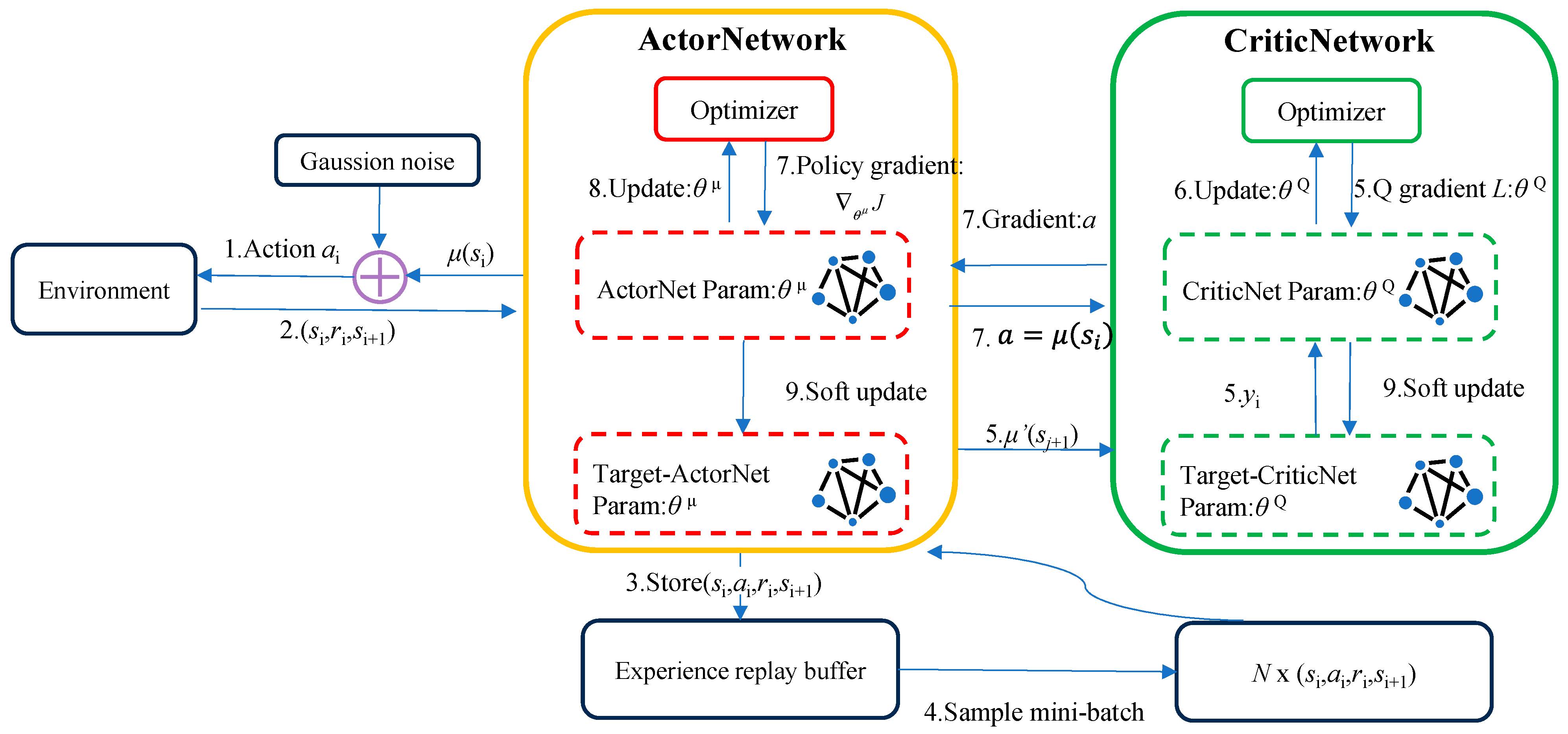
2.2.1. DDPG Algorithm

DDPG (Deep Deterministic Policy Gradient) is a depth deterministic strategy gradient algorithm. It is also a way to solve the problem of continuity control. It is a model-free, off-policy, or policy-based method. It solves the shortcoming that there is correlation before and after each parameter update of Actor-Critic neural network, which leads to the neural network only viewing the problem unilaterally, solving the shortcoming that DQN cannot be used for continuous action [30,31,32].

The structure of DDPG is like to Actor-Critic. DDPG can be divided into two major networks: strategy network and value network. DDPG continues the idea of fixed target network with DQN, and each network is subdivided into target network and reality network. However, the update of the target network is somewhat different, and its network structure is shown in Figure 5.

Figure 5. DDPG network structure.

DDPG consists of four networks: Actor current network, which is responsible for the iterative update of policy network parameters θ and the selection of current action A according to the current state S, which is used to interact with the environment to generate S’ and R’, the network update process is shown in Figure 6.

Figure 6. DDPG network update process.

Actor target network: it is responsible for selecting the optimal next action according to the next state sampled in the empirical playback pool, updating the network parameter θ′ by soft update. Critic network: responsible for the iterative update of value network parameter w and the calculation of Q value. Critic target network: responsible for calculating the Q′ part of the target Q value and soft updating the network parameter w′:

$$y_i=R+\gamma Q^{\prime }(S^{\prime },A^{\prime },w^{\prime }).$$

(3)

The neural network uses gradient backpropagation to change the parameters of the Actor and Critic networks:

According to the mathematical derivation in Sylver’s DPG paper [33], the strategy gradient update algorithm derived by adopting the off-policy training method according to the Monte Carlo method, when we randomly sample mini-batch data from replay memory buffers into the policy gradient formula described above, we can make an unbiased estimate of the expected value.

$$\nabla J(\theta )=\frac{1}{m}{\displaystyle \sum _{j=1}^m[{\nabla }_{a}Q(s_i,a_i,w){|}_{s=s_i,a={\pi }_{\theta (s)}}{\nabla }_{\partial }{\pi }_{\theta }(s){|}_{s=s_i}]}.$$

(4)

The loss function in the network is calculated using a method like supervised learning, which is usually calculated as the mean square error (MSE) calculation method.

$$J(w)=\frac{1}{m}{\displaystyle \sum _{j=1}^m{(y_i-Q(\varphi (S_j),A_j,w))}^2}.$$

(5)

DDPG uses a soft update method for network parameters, using the update coefficient τ, and only slightly modifies some parameters each time. Each iteration will modify the target network, and the algorithm can still maintain a certain stability.

$$\begin{array}{l}{w}^{\prime }\leftarrow \tau w+(1-\tau )w^{\prime }\\ {\theta }^{\prime }\leftarrow \tau \theta +(1-\tau ){\theta }^{\prime }\end{array}.$$

(6)

The target network parameter changes little and is used to calculate the gradient of the online network in the training process, which is relatively stable and easy to converge in training. However, with small parameter changes, the learning process is slow, and the use of a slowly updated target network can easily cause overestimation of Q value, which makes it difficult to converge the strategy. This defect is solved in TD3.

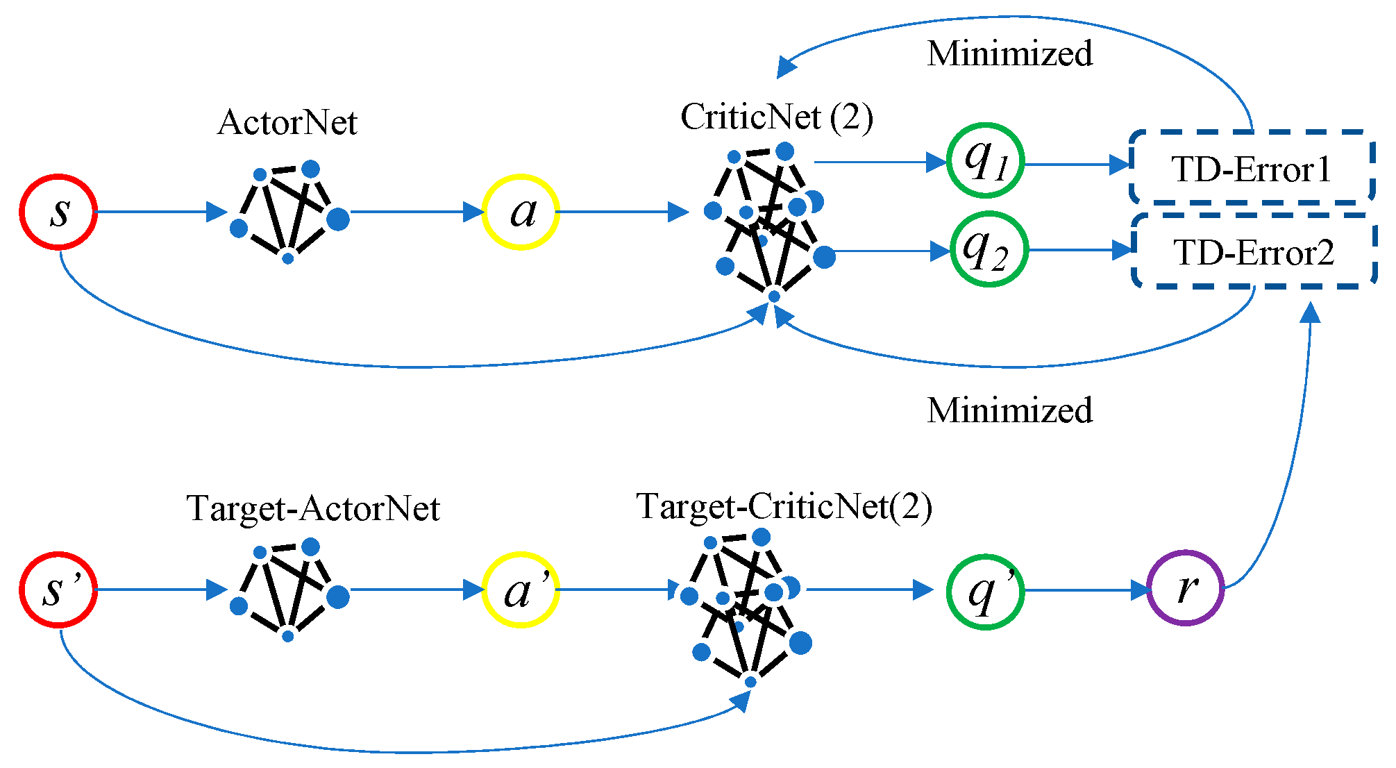
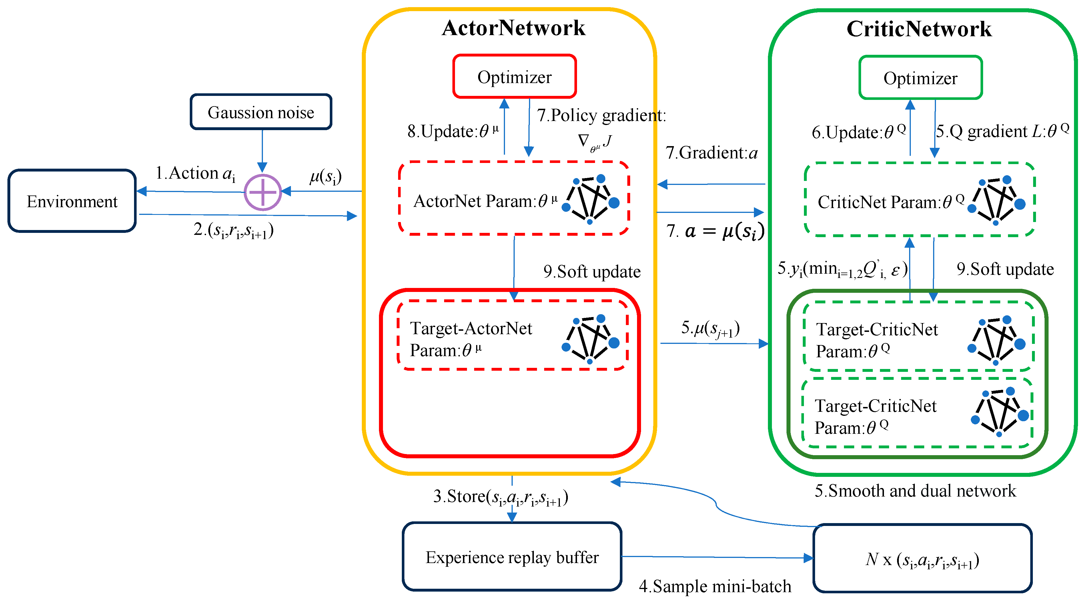
2.2.2. TD3 Algorithm

TD3 (Twin Delayed Deep Deterministic Policy Gradient Algorithm), an online off-policy deep RL method that is upgraded with DDPG is utilized to handle continuous control issues [34]. Essentially, the purpose of the TD3 algorithm is to include the Double Q-Learning algorithm into the DDPG algorithm. Combined with the concept of Double DQN, there are six networks in TD3, whose network structure is shown in Figure 7.

Figure 7. TD3 network structure.

The TD3 algorithm, which is based on the DDPG algorithm, proposes three fundamental technologies:

• Double network: Two sets of Critic networks are adopted, and the smaller value of the two is taken when calculating the target value, to suppress the overestimation problem of the network. According to Equation (3), the update mode of the target value Q′ can be known. The following Equation (7) represents the overestimation between the target value Q′ and the actual value Q*, when Q′ is close to y:

  $$Q^{\prime }\left(s^{\prime },a^{\prime }|{\theta }_i^{Q^{\prime }}\right)\ge Q^{*}(s^{\prime },a^{\prime }).$$

  (7)
• Target policy smoothing regularization: when the target value is calculated, the perturbation is added to the action of the next state, so that the value evaluation is more accurate:

  $$\begin{array}{c}y=r+\gamma {\min }_{i=1,2}Q\left(s^{\prime },a^{\prime }|{\theta }_i^{Q^{\prime }}+\epsilon |{\theta }_i^{Q^{\prime }}\right)\\ \epsilon ~clip(N(0,\sigma ),-c,c)\end{array}.$$

  (8)
• Soft update: After the Critic network is updated for several times, the Actor network is updated, to ensure that the Actor network training is more stable. A learning rate τ is introduced, the old target network parameters and the new corresponding network parameters are weighted averaged, and then assigned to the target network:

  $$\begin{array}{c}{\theta }^{Q_i^{\prime }}=\tau {\theta }^{Q_i}+(1-\tau ){\theta }^{Q_i^{\prime }}(i=1,2)\\ {\theta }^{{\mu }^{\prime }}=\tau {\theta }^{\mu }+(1-\tau ){\theta }^{{\mu }^{\prime }}\end{array}.$$

  (9)

The update process of TD3 algorithm is not much different from that of DDPG algorithm, and the main difference lies in the calculation method of the target value (Equation (3)). Where Actor networks are updated by maximizing cumulative expected returns (deterministic policy gradient), Critic1 and Critic2 networks are updated by minimizing the error between the evaluated value and the target value (MSE). All target networks are updated using soft update (Exponential Moving Average (EMA)). In the training phase, we sample a Batch size of data from the Replay Buffer, assuming that one sample of data is (s, a, r, s′), the update process of all networks is as follows:

Update the Critic1 and Critic2 network parameters, calculate the actions under the state $s^{\prime }$ using the Target Actor network:

$$a^{\prime }={\mu }^{\prime }(s^{\prime }|{\theta }^{{\mu }^{\prime }}).$$

(10)

Then, smooth regularization based on the target strategy, and add noise to the target action $a^{\prime }$, and calculate the target value based on the idea of dual network (Equation (8)), The parameters in the Critic1 and Critic2 networks are updated using the gradient descent algorithm to minimize the error between the evaluated value and the target value:

$${\theta }_i\leftarrow \arg {\min }_{{\theta }_i}{N}^{-1}{{\displaystyle \sum (y-Q_{{\theta }_i}(s,a))}}^2.$$

(11)

After updating the Critic 1 and Critic 2 networks step d, start updating the Actor network and calculate the actions in state $s$ using the Actor network, The gradient ascent algorithm is used to maximize q_new and update the Actor network. The TD3 network update process is shown in Figure 8.

$$\{\begin{array}{l}{a}_{new}=\mu (s|{\theta }^{\mu })\\ q_{new}=Q_1(s,a_{new}|{\theta }^{Q_1})\end{array}.$$

(12)

Figure 8. TD3 network update process.

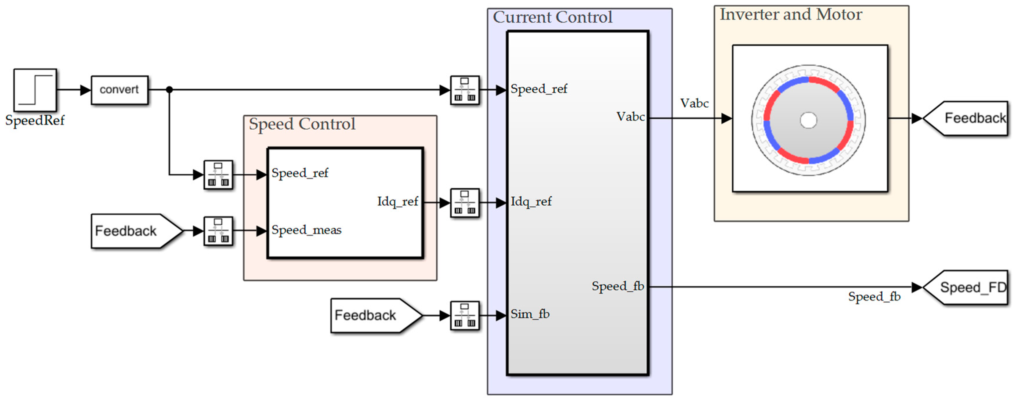
3. Establish Simulation Model

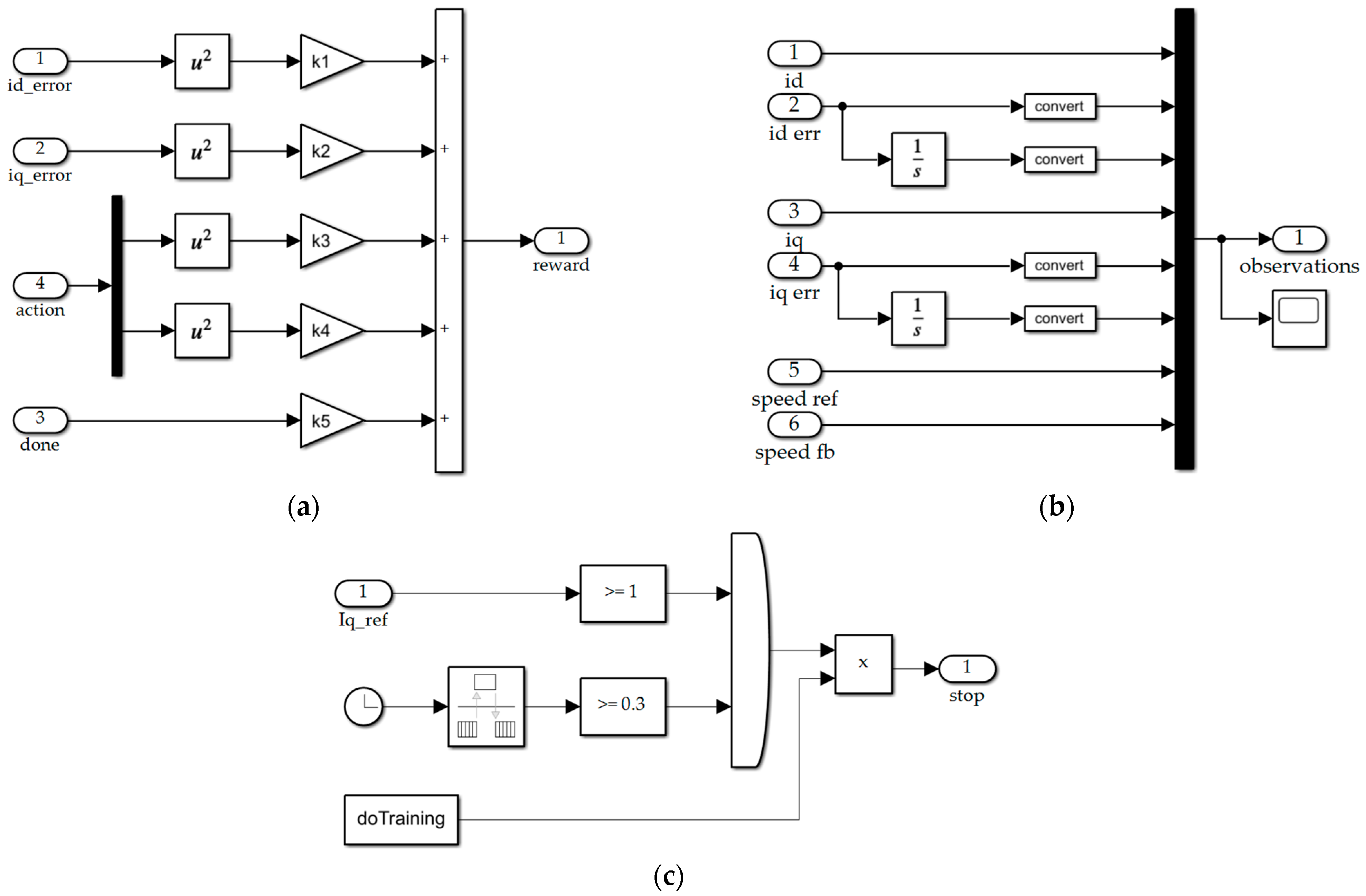
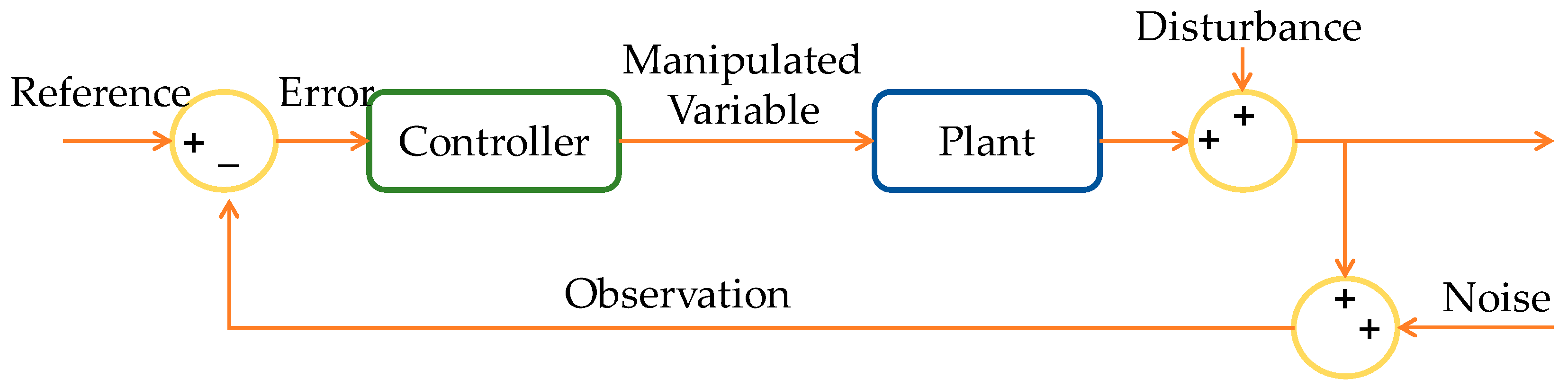
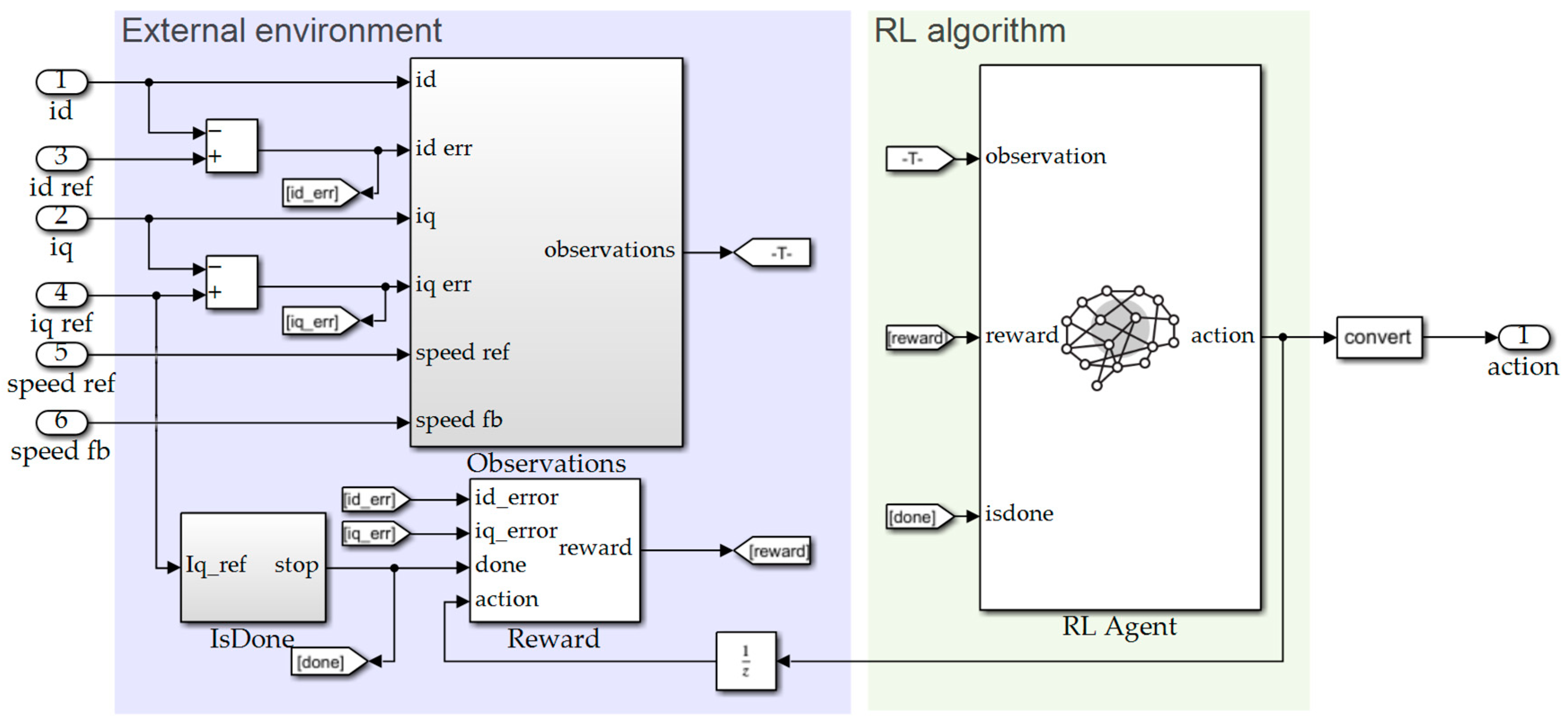
3.1. Create Environment

A Simulink model of the FOC control architecture is constructed, as shown below in Figure 9, which includes two control loops: the external speed loop and the internal current loop. The outer ring is realized in the speed control subsystem, while the current ring subsystem mainly changes the speed and torque of the motor by controlling the current of the two axes. Using the output current signal corresponding to the output voltage, the appropriate PWM signal is generated to adjust the semiconductor switch of the inverter, thereby driving the PMSM to achieve the required torque and flux.

Figure 9. PMSM RL-FOC control program construction.

The current loop consists of the following components: three-phase motor current acquisition; Clarke transformation; Park transformation; and a current loop controller (RL controller). This research focuses on the RL controller (shown below in Figure 10), which is primarily made up of external and RL environments. Figure 11 depicts the vector observer (a), reward function (b), and cutoff conditions (c).

Figure 10. RL framework.

Figure 11. RL learning and training structure. From left to right, (a) Reward function; (b) Observation vector; (c) Termination condition.

The PMSM model’s related parameters are listed in Table 2 below.

Table 2. Main parameters of PMSM model.

Term Name	Symbol	Value
Pole pairs	p	7
Torque constant	Kt	0.0583 N·m/A
Friction coefficient	B	7.01 × 10−5 Kg·m2/s
Rate current	Ir	7.26 A
Stator resistor	Rs	0.293 Ω
D-Axis inductance value	Ld	0.877 mH
Q-Axis inductance value	Lq	0.777 mH
Inertia	J	0.0083 Kg·m2
Max speed	Vmax	4300 RPM
Position offset	Po	0.165
QEP encoder slits	Qs	4096

The motor module is simulated and analyzed. The motor characteristic curve is shown in Figure 12 below.

Figure 12. Motor characteristic curve. From left to right, (a) Torque–Speed characteristics; (b) Power–Speed characteristics; (c) I_dq–Speed characteristics; (d) I_pear–Speed characteristics.

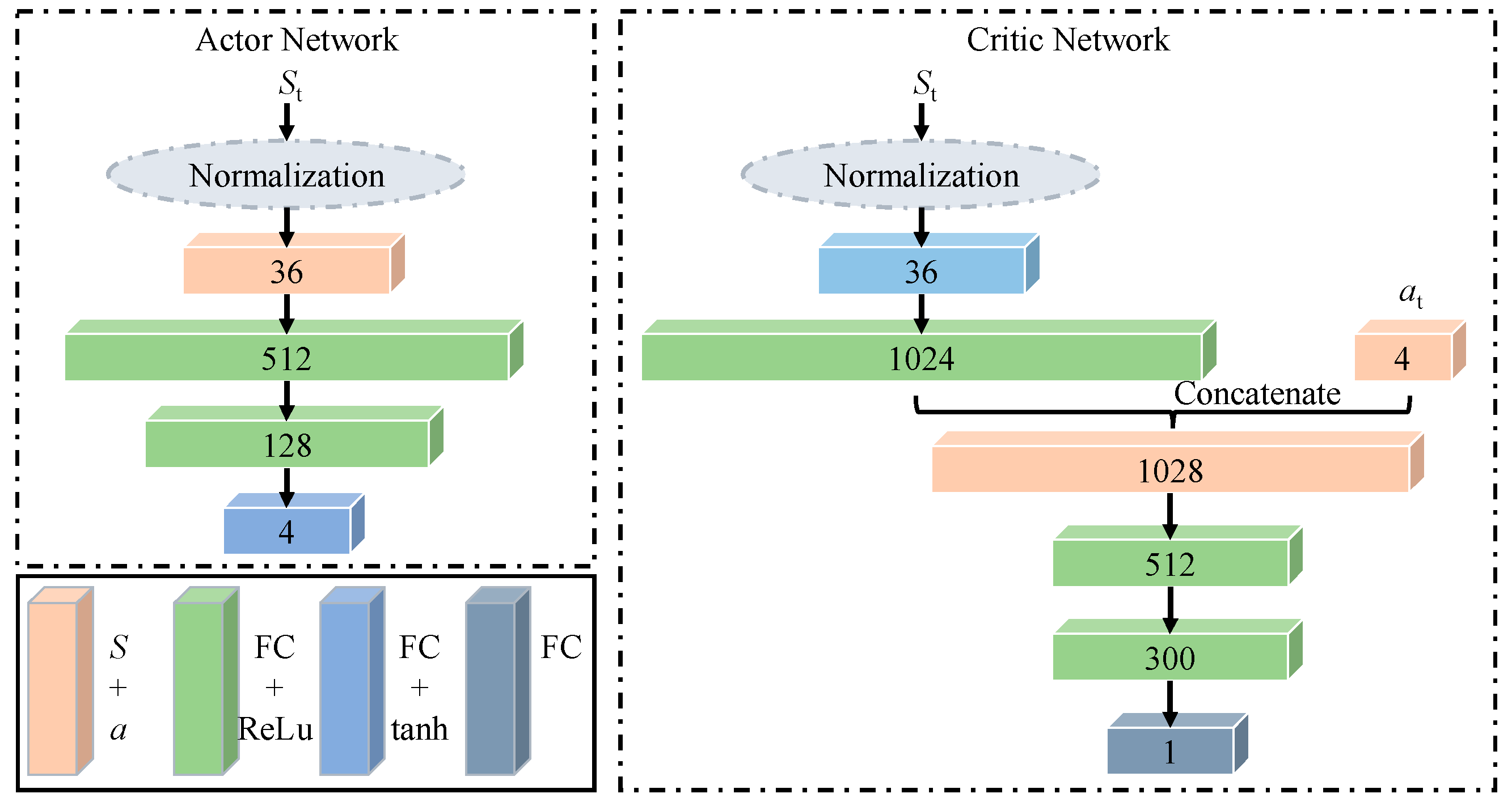
3.2. Create RL Module

The RL agent network is built in the previously developed Simulink environment. The network form of the TD3 algorithm is shown in Figure 13. Table 3 defines important parameters related to training. After setting the relevant parameters, the model is trained offline.

Figure 13. RL learning and training structure.

Table 3. The setting of hyperparameters.

Hyperparameter	Symbol	Value
Random seed	αr	1
Maximal set	M	2000
Maximum sub-step size per episode	T	5000
Sample Time	Ts	2 × 10−4
Time of simulation	Tf	3
Experience Buffer Length	Β	2 × 106
Quantity of batch	N	250
Threshold of gradient	ε	1
Learning rate of Actor network	La	0.001
Learning rate of Critic network	Lc	0.0002
Noise of exploration	e	0.1
Delayed updating	D	2
L2 Regularization Factor	L2	0.001
Target Update Frequency	wt	10
Factor of discount	γ	0.995
Rate of soft renewal	τ	0.01

After the program sets the hyperparameters, the training begins. The time of training is determined by the complexity of the model. The parallel computing toolbox in MATLAB is used to calculate the RL control model quickly, so that the program and model can run in interactive and batch mode, and the training time is greatly shortened.

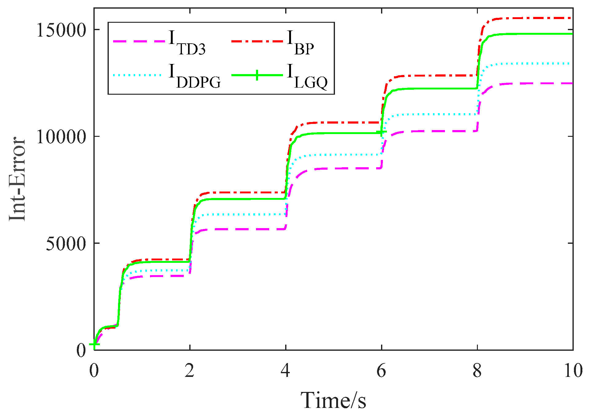
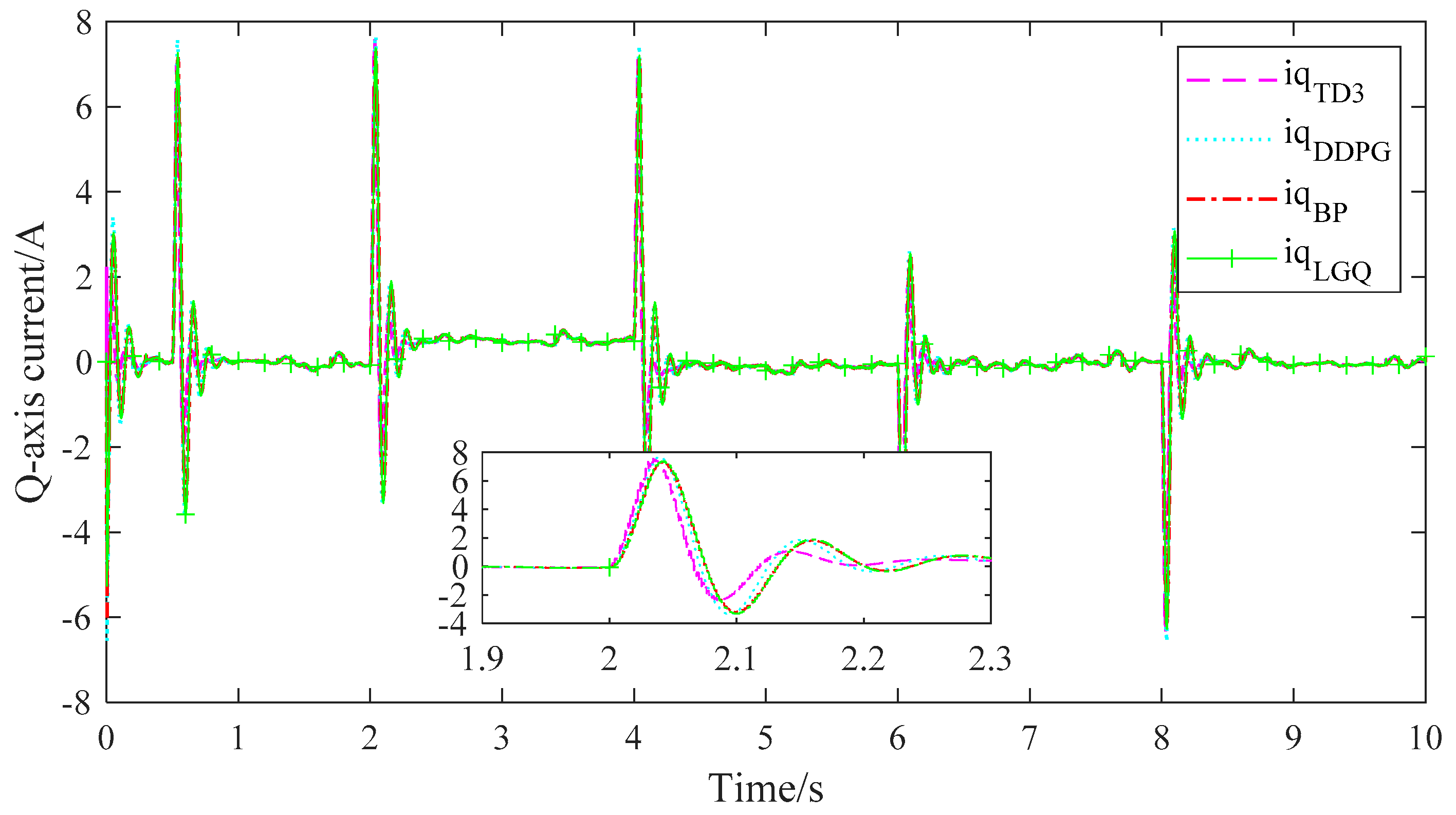
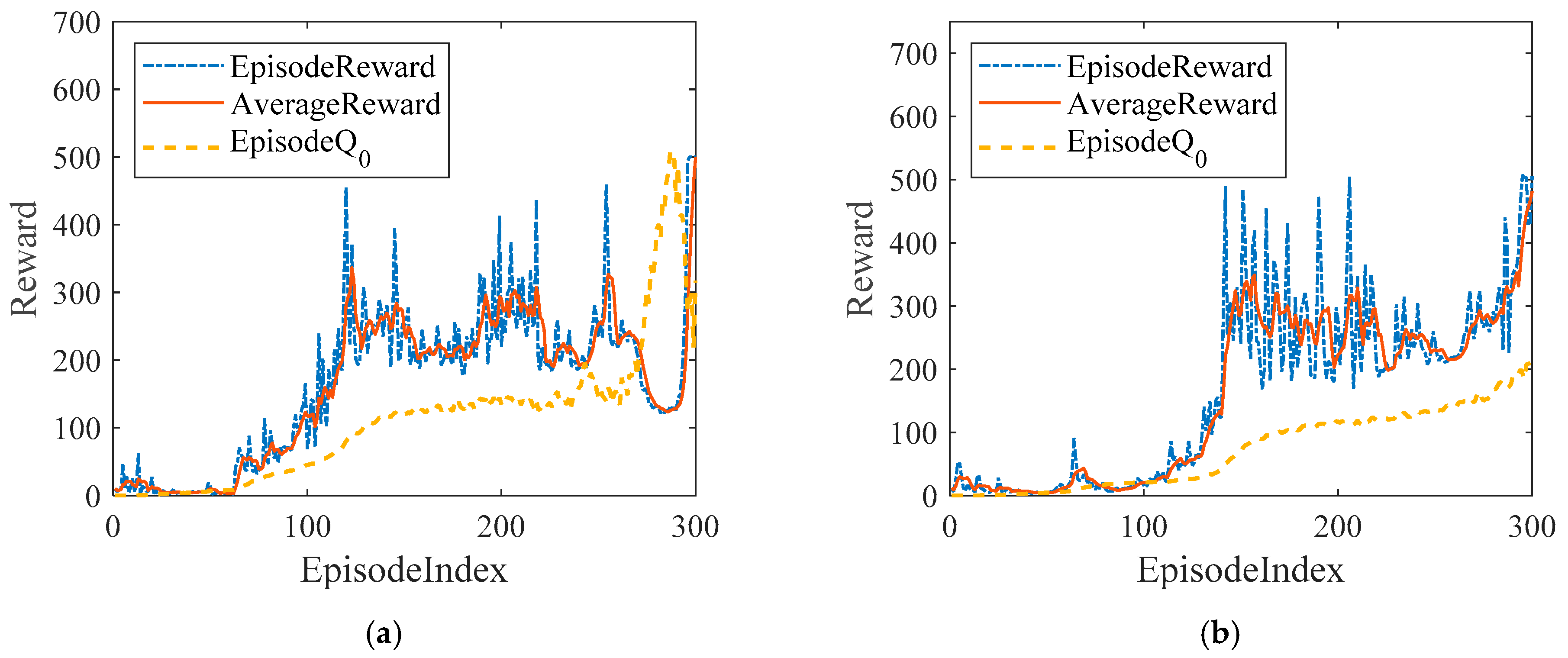
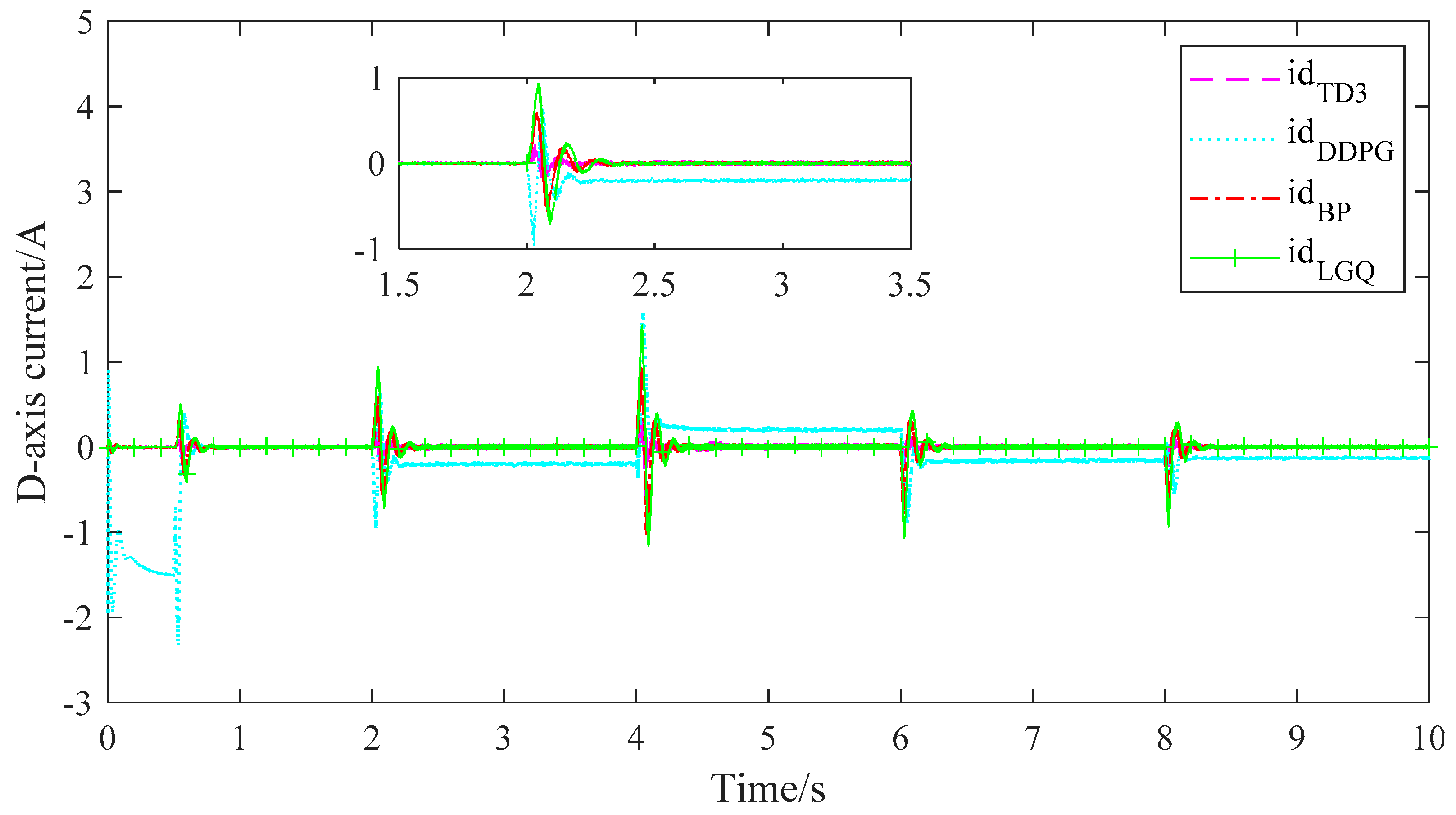
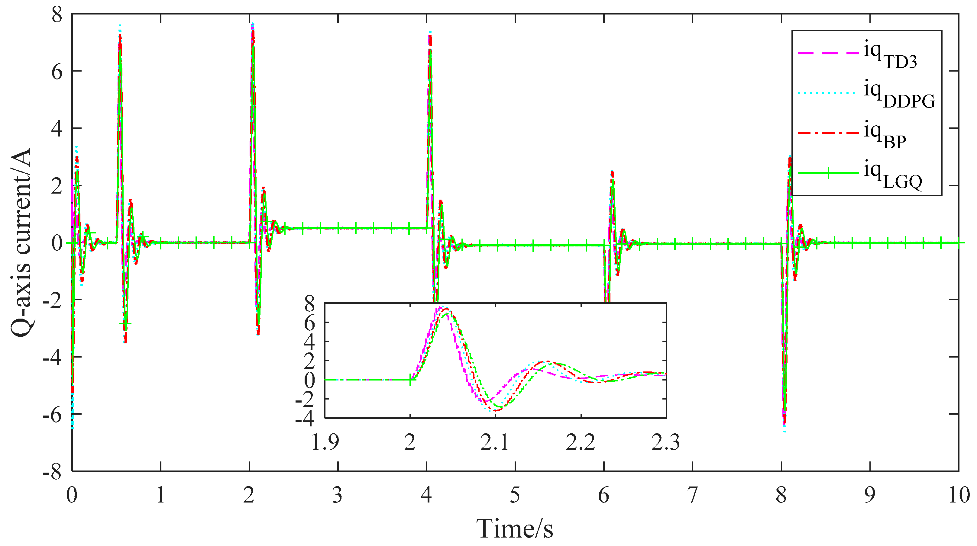
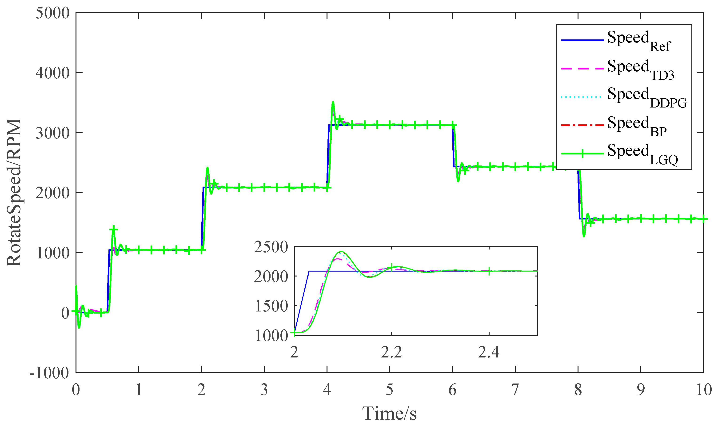
4. Comparison of Simulation Results

When the number of iterations reaches 300, the training ends. It can be seen from the Figure 14a, the average reward at the end of TD3 was 541 and DDPG was 520. As the estimate of long-term discount at the beginning of each episode, Q₀ is closer to the real long-term value. As can be seen from the Figure 14b, Q₀ under TD3 algorithm training is 545, while the maximum value of Q₀ under DDPG algorithm is 210, which proves that PMSM current loop control under TD3 algorithm training will have better results. In terms of training time, TD3 training ended in 3 min and 56 s and DDPG training ended in 5 min and 55 s. From the training results and training time, TD3 training reward value is higher and training time is shorter, and therefore, more suitable for RL control in the current loop.

Figure 14. Training result. From left to right, (a) DDPG training results; (b) TD3 training results.

To evaluate the real control performance of the training network, the above TD3-RL control is compared with DDPG-RL control, linear quadratic Gauss (LQG) control, and BP network controller in simulation tests.

The simulation is mainly to verify whether this control method can make the motor stable in the starting stage, during increasing and decelerating processes, and the loading and unloading of Work reliably. To better verify the reliability of the algorithm, a variety of working conditions are reflected in a simulation experiment. First, let the motor start no-load to the given speed of 1000 r/min, the start time is very short, the stepped speed rises, and then increase the load torque of 0.03 N·m at 2 s, reduce the given load to 0 N·m at 4 s, and increase the speed to 3100 r/min. Then, the speed drops step by step. The simulation experiment results are shown in Figure 15.

Figure 15. Motor speed under different algorithms.

As can be seen from Figure 16, the error fluctuation is particularly obvious, and the cumulative error of TD3 (the error integral under each simulation step) is smaller than that of the other three methods. As can be seen below from Table 4, compared with BP and LQG, the error of the two RL algorithms in signal tracking is smaller, while the step signal rise time of the system under TD3 algorithm is 0.1 s, the overshoot is 7.38%, and the stabilization time is 18.54% less than that of DDPG algorithm.

Figure 16. Error integral curve.

Table 4. Performance comparison under different control algorithms.

Performance Parameters	BP	LQG	DDPG	TD3
Settling time	0.98 s	0.82 s	0.89 s	0.8 s
Risetime	0.2 s	0.19 s	0.15 s	0.1 s
Undershoot	15.03%	12.7%	12.21%	7.76%

Figure 17 and Figure 18 show the corresponding D-axis current and Q-axis current under the four algorithms.

Figure 17. D-axis current.

Figure 18. Q-axis current.

The stator current amplitude is constant during the motor starting process, because the deviation between the given speed and the current speed value is too large, so that the outer loop PI of the speed is saturated. Due to the limiting effect of the controller, the given current of the output Q-axis is the limiting value, and the current of the D-axis is controlled by i_d = 0, so the amplitude of the stator three-phase current is constant. It can be seen from Figure 17 that TD3 algorithm has the smallest i_d fluctuation when torque is applied, and i_q response speed is faster than other algorithms. TD3-FOC has faster speed and torque current response than the other three algorithms in the start-up stage, loading stage, and unloading stage, and has better control performance.

5. Experiment

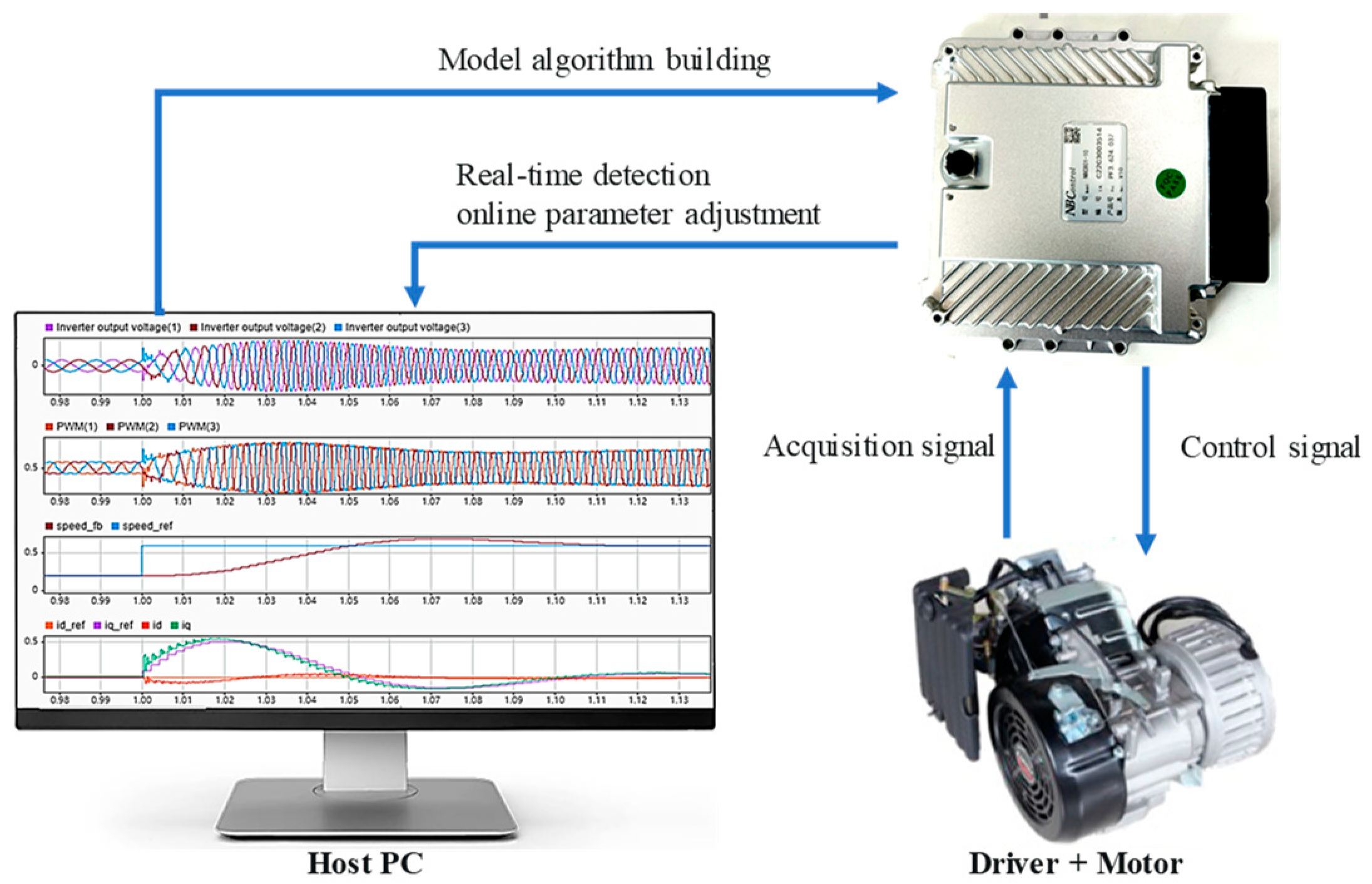
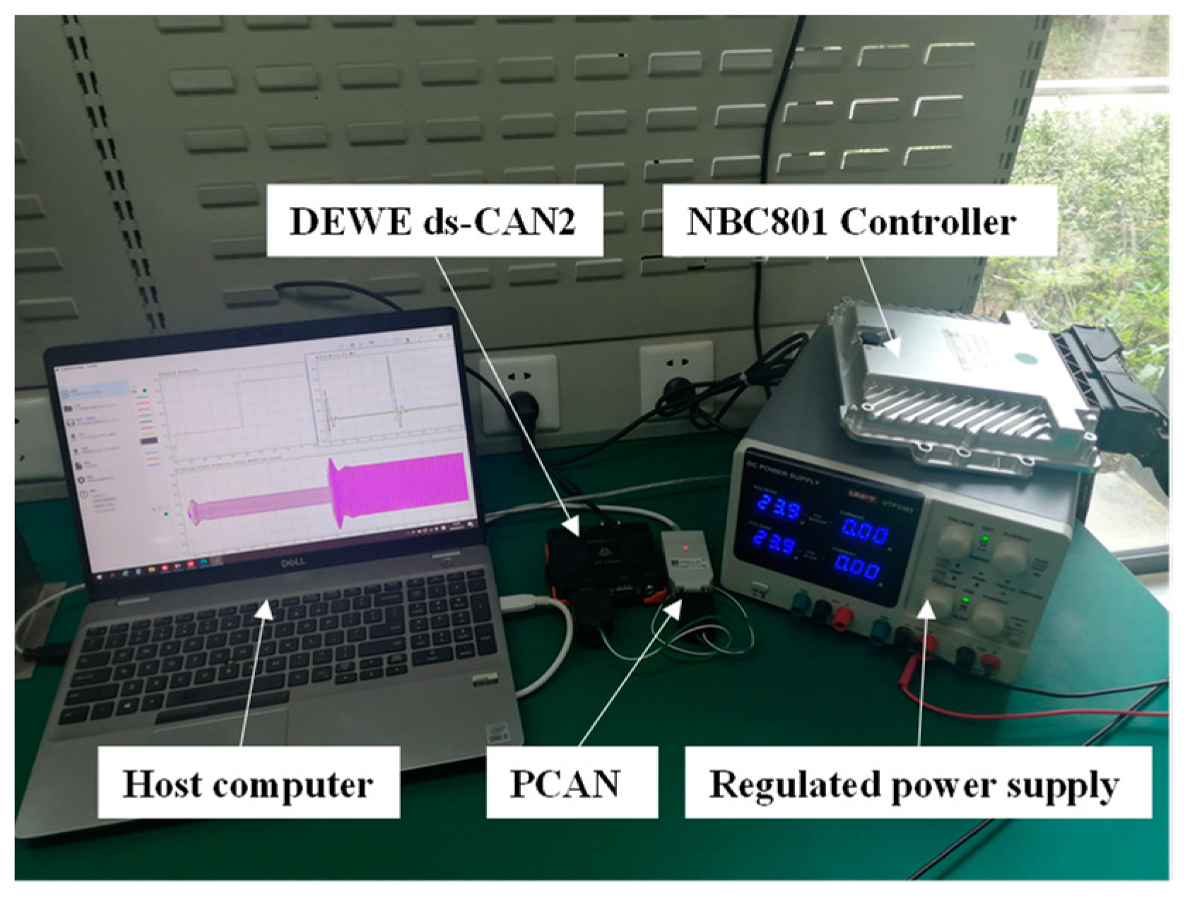
5.1. Real-Time Simulation

To validate the deep learning workflow, we used Simulink and Controller. The trained RL agent is deployed to the controller and the DRL compiled C code is tested in real time. By measuring the analog signal output of the controller, the control effect of the four algorithms on the current loop are compared. The working process is shown below in Figure 19.

Figure 19. Real-time simulation workflow.

5.2. Rapid Control Prototype

Rapid Control Prototype (RCP) is a technique to adjust control algorithms on hardware prototype. The supplied algorithm model can be executed on a real-time controller connected to the actual I/O by using the interface module in conjunction with the Simulink platform to import mathematical models rapidly and easily.

RCP can cut down on the amount of time needed for debugging, hardware adaptation, code translation, and other tasks during the learning or development phase. The actual object can be controlled and tested once the algorithm has been swiftly downloaded and implemented through the fast control prototype simulator. The RCP technique has the following benefits over the conventional method:

(1)

Easy deployment: quick and efficient deployment of control algorithms, which lessens the need for subsequent development.

(2)

Simple coordination: by connecting to the controlled object, any issues with the control technique can be rapidly identified. Offline digital simulation is performed before the algorithm model is downloaded to the control board in C for further debugging.

(3)

High degree of adaptability: the RCP simulation platform’s powerful performance and abundant resources can suit a variety of research and development objectives.

Based on the concept of RCP technology, the RL controller is downloaded to the controller through the code compilation tool for online data monitoring, verifying the correctness of the simulation results and greatly reducing the test time.

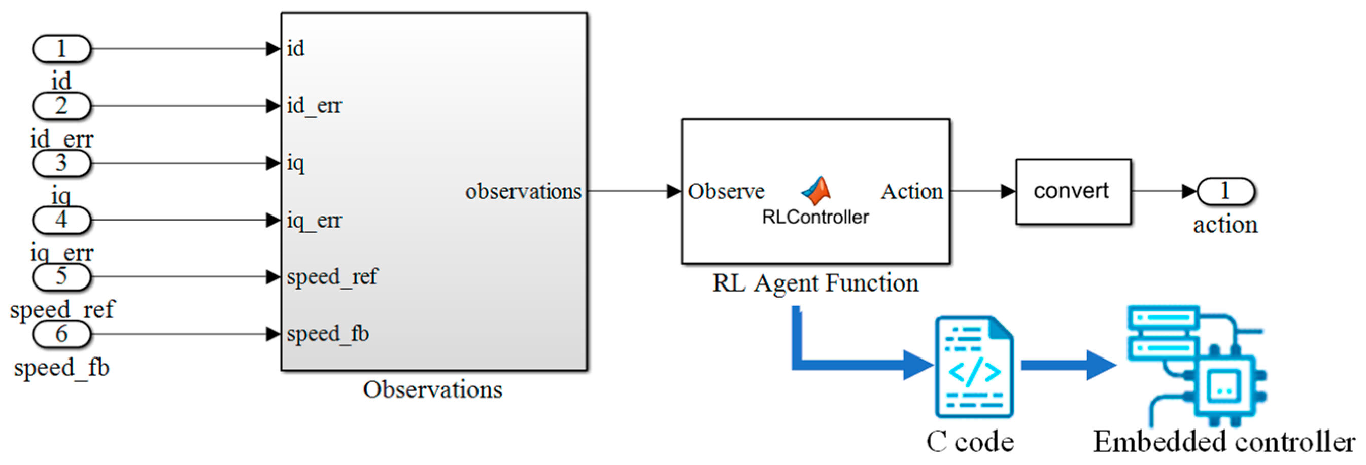
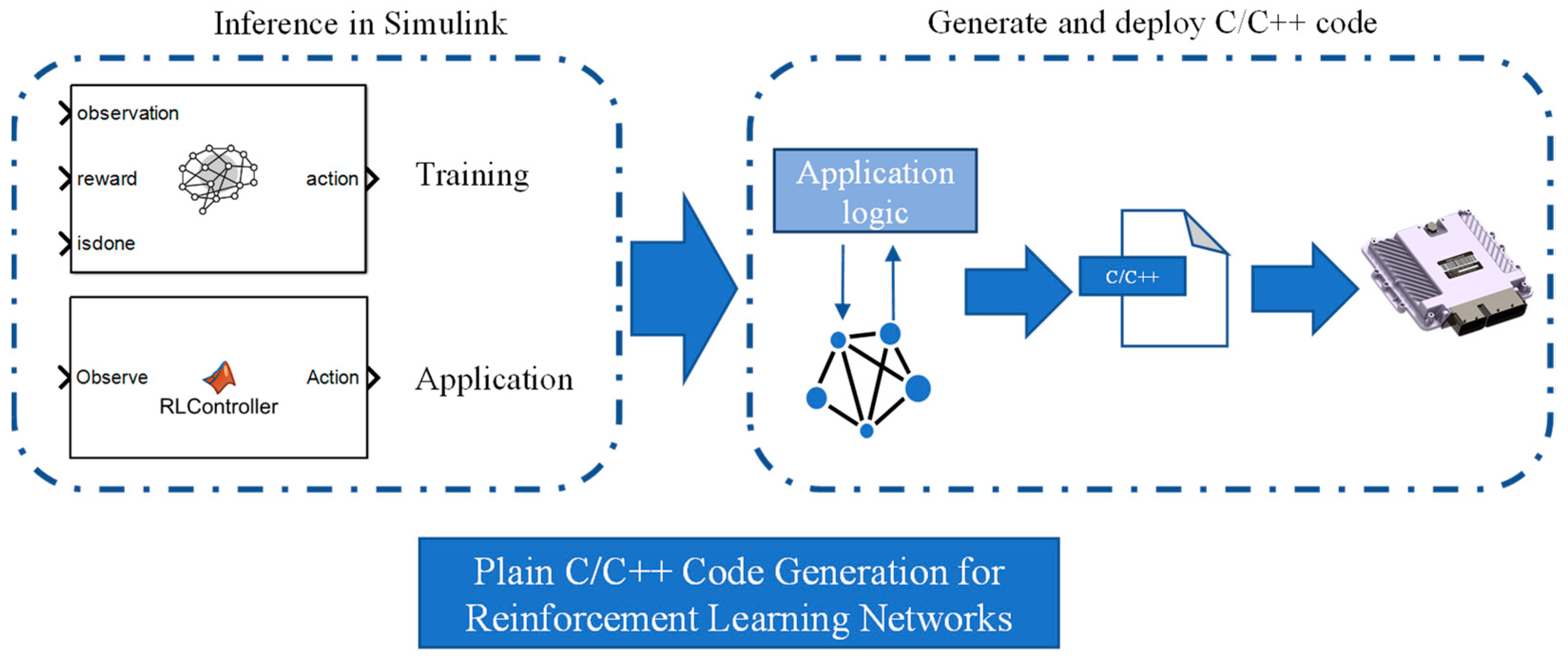
5.3. Code Generation

Machine learning is a complex process that requires a significant amount of processing to train models, yet has memory and compute restrictions for embedded devices. We first trained the agent in the simulated environment using the MATLAB Coder tool chain, which reduced the time and effort required for producing, redeploying, and testing C/C ++ code. The finalized code was then deployed with the help of code generating tools. Figure 20 depicts the workflow.

Figure 20. RL module conversion compilation.

Pre-trained agents were loaded and tested in embedded controllers using the RL Agent block, but we discovered that this functional module did not permit direct code generation. We constructed a MATLAB function block and swap out the existing RL training Settings to do deep learning reasoning in Simulink and produce code to download to the controller for testing. The function block takes advantage of the new deep learning function to do reasoning on the training strategy in Simulink. The trained DRL network actor, the agent data file, and the policy evaluation function are all contained in the same folder and are generated by the interface function which is constructed to generate the interface function. We then developed and deployed whole Simulink real-time apps on embedded hardware by utilizing deep learning networks’ common C/C++ code generating capabilities. Figure 21 depicts the main steps in creating code.

Figure 21. RL Control module.

Replace the smart block with the MATLAB Function block. Since it has been trained, it does not need the observation vector and cutoff module. The PWM analog signal output port of NBC801 is connected at the signal output end to facilitate data acquisition with DEWE. The hardware test scheme is shown in Figure 22.

Figure 22. Rapid control prototype experiment of RL.

This experiment uses NBC801 as the controller. NBC801 is a secondary programmable embedded controller with benefits in a wide range of temperatures and voltages as well as excellent seismic performance. Its IP67 level of protection allows it to fully satisfy the application requirements for severe working environments. Table 5 lists the hardware parameters of NBC801. Data acquisition, control output, data storage, CAN communication, RS232 communication, and other hardware tasks have all been integrated into the controller. To output the control signal, we use the IO terminal library built on the Simulink platform. The output signal is scaled, configured as a proportional output, and the DEWE data collector is used to gather the signal data to confirm that the output terminal of the controller is within the operating range.

Table 5. Mainframe’s technical specifications of NBC801.

Type	Technical Specifications
MCU	Mononuclear & 32 bit & 600 MHz
Current operating system	Simulink & CODESYS
Memory space	512 KB × RAM Flash 16 MB
Interface	1 × USB 3.0 & 2 × USB 2.0
Computer interface	4 × CAN, 1 × RS 232
Power supply	+9–+32 V
Port channel number	20 × AI(0–5 V/0–20 mA), 4 × AI(0–5 V/32 V), 2 × AI(0–2.2 kΩ)
	10 × PI
	8 × DO
	30 × PWM
Dimension	242 × 234 × 40 mm

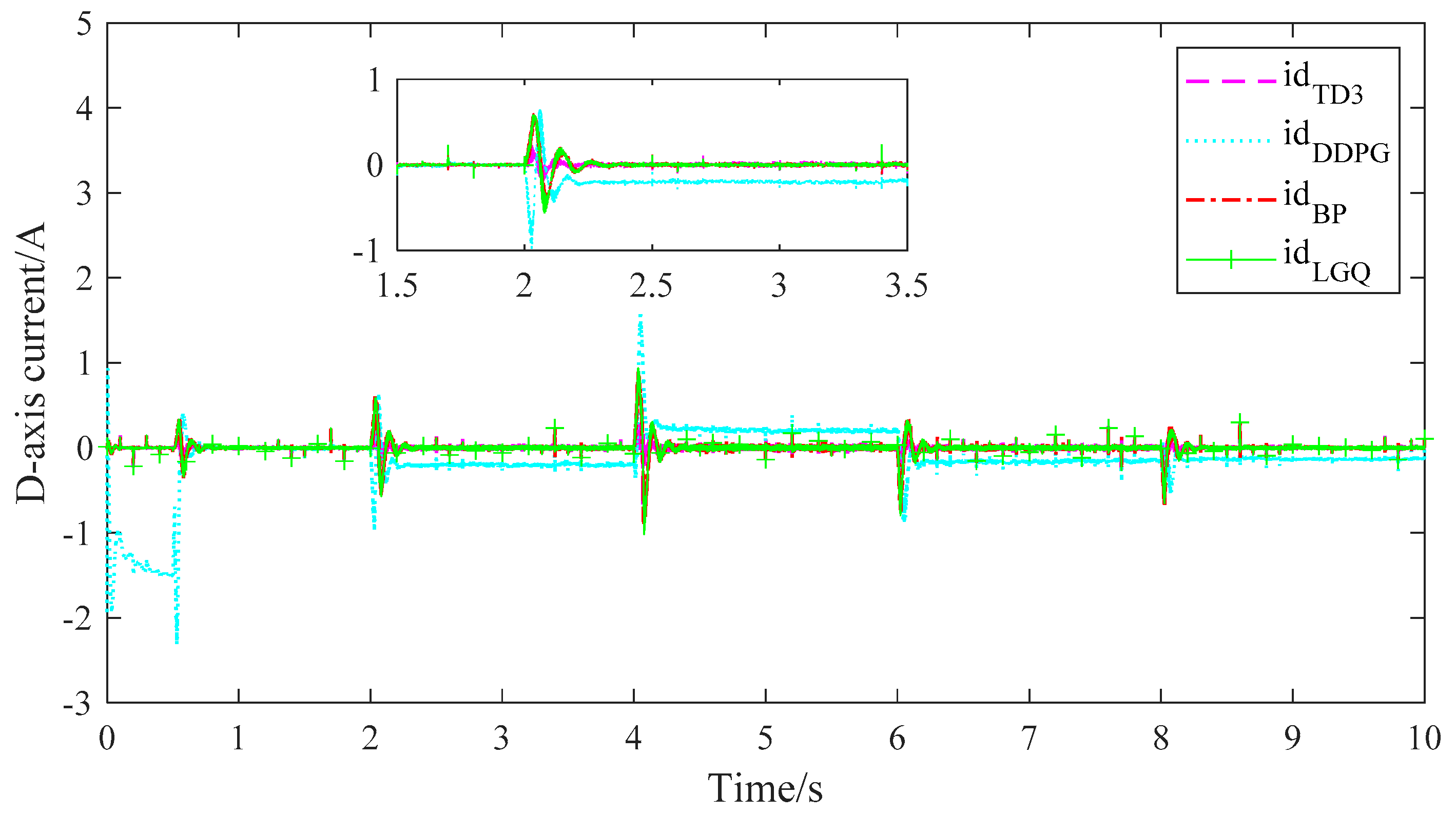
5.4. Result Analysis

Through the DEWE DS-CAN2 data acquisition device, we view the output signal after the generated application has been loaded and launched on the embedded controller.

During the initial stage, the speed increased rapidly and steadily (Figure 23). When the rotational speed is stable at 1000 r/min, the overshoot n1 ≈ 100 r/min is reached. When the motor is suddenly loaded with 0.03 N·m, the speed overshoot time of PMSM starting stage under TD3 algorithm is about 0.2 s. When loading, the speed regulation time is about 0.3 s. At this time, the Q-axis current can quickly track the reference signal and reach stability quickly, while the D-axis current is not affected by the Q-axis current and always fluctuates near zero, indicating that the TD3-FOC control has good dynamic steady-state control performance. Figure 24 error integral curve shows the speed tracking effect of the four algorithms.

Figure 23. Motor speed under different algorithms.

Figure 24. Error integral curve.

Figure 25 and Figure 26 show the dynamic response process of D-axis and Q-axis current in the speed regulation process of the four algorithms, respectively. As can be seen from the figure, the i_d and i_q fluctuations of TD3-FOC controlled PMSM when the load is applied are smaller than those of the other three algorithms; the experimental results are consistent with the simulation results.

Figure 25. D-axis current.

Figure 26. Q-axis current.

We can see that the PMSM model controlled by TD3-FOC performs well in terms of speed tracking and current tracking output of the model, which indicates that the code of TD3-FOC algorithm is compiled and implemented successfully in the controller, and it has produced a good current control effect.

6. Conclusions

This paper presents a current control algorithm based on TD3-FOC. The PMSM model and RL model framework are established, and RL controller block is used to replace the current loop controller to update the old model. In addition, vector observer, reward function, and cutoff function are defined for training current control, TD3 and DDPG algorithms are trained, BP and LQG are trained under the same conditions, and the results of the four algorithms in PMSM current loop control are compared by simulation and experiment. The results show that the velocity tracking performance of vector control is improved when the stator current is controlled by TD3-FOC. Finally, through rapid prototyping experiment, the trained network is compiled into C code and downloaded to the embedded controller. The data acquisition device collects the output signal of the controller, which is consistent with the simulation results, and the correctness of the control scheme is verified.

References

1. Sarlioglu, B.; Morris, C.T. More Electric Aircraft: Review, challenges, and opportunities for commercial transport aircraft. IEEE Trans. Transp. Electron. 2015, 1, 54–64. [Google Scholar] [CrossRef]
2. Zhang, M.; Mccarthy, Z.; Finn, C.; Levine, S.; Abbeel, P. Learning deep neural network policies with continuous memory states. In Proceedings of the International Conference on Robotics and Automation, Stockholm, Sweden, 16 May 2016; pp. 520–527. [Google Scholar]
3. Lenz, I.; Knepper, R.; Saxena, A. DeepMPC: Learning deep latent features for model predictive control. In Proceedings of the Robotics Scienceand Systems, Rome, Italy, 13–17 July 2015; pp. 201–209. [Google Scholar]
4. Bolognani, S.; Bolognani, S.; Peretti, L.; Zigliotto, M. Design and implementation of model predictive control for electrical motor drives. IEEE Trans. Ind. Electron. 2009, 56, 1925–1936. [Google Scholar] [CrossRef]
5. Tiwari, A.; Singh, S.; Singh, S. PMSM Drives and its Application: An Overview. Recent Adv. Electr. Electron. Eng. 2023, 16, 4–16. [Google Scholar]
6. Beaudoin, M.; Boulet, B. Improving gearshift controllers for electric vehicles with reinforcement learning. Mech. Mach. Theory 2022, 169, 104654. [Google Scholar] [CrossRef]
7. Chang, X.; Liu, L.; Ding, W.; Liang, D.; Liu, C.; Wang, H.; Zhao, X. Novel nonsingular fast terminal sliding mode control for a PMSM chaotic system with extended state observer and tracking differentiator. J. Vib. Control 2017, 23, 2478–2493. [Google Scholar] [CrossRef]
8. Chen, J.; Yao, W.; Ren, Y.; Wang, R.; Zhang, L.; Jiang, L. Nonlinear adaptive speed control of a permanent magnet synchronous motor: A perturbation estimation approach. Control Eng. Pract. 2019, 85, 163–175. [Google Scholar] [CrossRef]
9. Dai, C.; Guo, T.; Yang, J.; Li, S. A disturbance observer-based current-constrained controller for speed regulation of PMSM systems subject to unmatched disturbances. IEEE Trans. Ind. Electron. 2021, 68, 767–775. [Google Scholar] [CrossRef]
10. Guo, T.; Sun, Z.; Wang, X.; Li, S.; Zhang, K. A simple current-constrained controller for permanent-magnet synchronous motor. IEEE Trans. Ind. Inf. 2019, 15, 1486–1495. [Google Scholar] [CrossRef]
11. Xu, Q.; Zhang, C.; Zhang, L.; Wang, C. Multi-objective Optimization of PID Controller of PMSM. Control Sci. Eng. 2014, 2014, 471609. [Google Scholar]
12. Zhang, W.; Cao, B.; Nan, N.; Li, M.; Chen, Y. An adaptive PID-type sliding mode learning compensation of torque ripple in PMSM position servo systems towards energy efficiency. ISA Trans. 2020, 110, 258–270. [Google Scholar] [CrossRef] [PubMed]
13. Lu, W.; Cheng, K.; Hu, M. Reinforcement Learning for Autonomous Underwater Vehicles via Data-Informed Domain Randomization. Appl. Sci. 2023, 13, 1723. [Google Scholar] [CrossRef]
14. Zhang, L.; Li, D.; Xi, Y.; Jia, S. Reinforcement learning with actor-critic for knowledge graph reasoning. Sci. China Inf. Sci. 2020, 63, 1–3. [Google Scholar] [CrossRef]
15. Zhao, B.; Liu, D.; Luo, C. Reinforcement learning-based optimal stabilization for unknown nonlinear systems subject to inputs with uncertain constraints. IEEE Trans. Neural Netw. Learn. Syst. 2020, 31, 4330–4340. [Google Scholar] [CrossRef] [PubMed]
16. Zhang, S.; Li, Y.; Dong, Q. Autonomous navigation of UAV in multi-obstacle environments based on a Deep Reinforcement Learning approach. Appl. Soft. Comput. 2022, 115, 108194. [Google Scholar] [CrossRef]
17. Nicola, M.; Nicola, C.; Selișteanu, D.; Ionete, C. Control of PMSM Based on Switched Systems and Field-Oriented Control Strategy. Automation 2022, 3, 646–673. [Google Scholar] [CrossRef]
18. Hong, Z.; Xu, W.; Lv, C.; Ouyang, Q.; Wang, Z. Control Strategy of Deep reinforcement Learning-PI Air Rudder Servo System based on Genetic Algorithm optimization. J. Mech. Electron. Eng. 2019, 40, 1071–1078. [Google Scholar]
19. Yang, C.; Wang, H.; Zhao, J. Model-free optimal coordinated control for rigidly coupled dual motor systems based on reinforcement learning. IEEE/ASME Trans. Mechatron. 2023, 16, 1–13. [Google Scholar]
20. Pesce, E.; Montana, G. Learning multi-agent coordination through connectivity-driven communication. Mach. Learn. 2022, 112, 483–514. [Google Scholar] [CrossRef]
21. Li, Y.; Wu, B. Software-Defined Heterogeneous Edge Computing Network Resource Scheduling Based on Reinforcement Learning. Appl. Sci. 2022, 13, 426. [Google Scholar] [CrossRef]
22. Huo, L.; Tang, Y. Multi-Objective Deep Reinforcement Learning for Personalized Dose Optimization Based on Multi-Indicator Experience Replay. Appl. Sci. 2022, 13, 325. [Google Scholar] [CrossRef]
23. Wu, C.; Pan, W.; Staa, R.; Liu, J.; Sun, G.; Wu, L. Deep reinforcement learning control approach to mitigating actuator attacks. Automatica 2023, 152, 110999. [Google Scholar] [CrossRef]
24. Jean, C.; Kyandoghere, K. Systems Science in Engineering for Advanced Modelling, Simulation, Control and Optimization; CRC Press: Boca Raton, FL, USA, 2019; pp. 34–50. [Google Scholar]
25. Riazollah, F. Servo Motors and Industrial Control Theory; Springer: Berlin/Heidelberg, Germany, 2014; pp. 21–40. [Google Scholar]
26. GonzálezRodríguez, A.; BarayArana, R.; RodríguezMata, A.; RobledoVega, I.; Acosta, C. Validation of a Classical Sliding Mode Control Applied to a Physical Robotic Arm with Six Degrees of Freedom. Processes 2022, 10, 2699. [Google Scholar] [CrossRef]
27. Dhulipati, H.; Ghosh, E.; Mukundan, S.; Korta, P.; Tjong, J.; Kar, N. Advanced design optimization technique for torque profile improvement in six-phase PMSM using supervised machine learning for direct-drive EV. IEEE Trans. Energy Convers. 2019, 34, 2041–2051. [Google Scholar] [CrossRef]
28. Zhao, X.; Ding, S. Research on deep rein-forcement learning. Comput. Sci. 2018, 45, 1–6. [Google Scholar]
29. Wen, G.; Philip, C.C.L.; Sam, G.S.; Yang, H.; Liu, X. Optimized adaptive nonlinear tracking control using actor–critic rein-forcement learning policy. IEEE Trans. Ind. Inf. 2019, 15, 4969–4977. [Google Scholar] [CrossRef]
30. Thuruthel, T.G.; Shih, B.; Laschi, C.; Tolley, M.T. Soft robot perception using embedded soft sensors and recurrent neural networks. Sci. Rob. 2019, 4, 1488–1497. [Google Scholar] [CrossRef] [PubMed]
31. Zhang, F.; Li, J.; Li, Z. A TD3-based multi-agent deep reinforcement learning method in mixed cooperation-competition environment. Neurocomputing 2020, 411, 206–215. [Google Scholar] [CrossRef]
32. Yao, J.; Ge, Z. Path-Tracking Control Strategy of Unmanned Vehicle Based on DDPG Algorithm. Sensors 2022, 22, 7881. [Google Scholar] [CrossRef]
33. Silver, D.; Lever, G.; Heess, N.; Degris, T.; Wierstra, D.; Riedmiller, M. Deterministic Policy Gradient Algorithms. OpenAI 2014, 12, 387–395. [Google Scholar]
34. Vrabie, D.; Vamvoudakis, K.; Lewis, F. Optimal Adaptive Control and Differential Games by Reinforcement Learning Principles. IET Digit. Libr. 2012, 3, 1–47. [Google Scholar]