Generation of Achievable Three-Dimensional Trajectories for Autonomous Wheeled Vehicles via Tracking Differentiators

Abstract

Planning an achievable trajectory for a mobile robot usually consists of two steps: (i) finding a path in the form of a sequence of discrete waypoints and (ii) transforming this sequence into a continuous and smooth curve. To solve the second problem, this paper proposes algorithms for automatic dynamic smoothing of the primary path using a tracking differentiator with sigmoid corrective actions. Algorithms for setting the gains of the differentiator are developed, considering a set of design constraints on velocity, acceleration, and jerk for various mobile robots. When tracking a non-smooth primary path, the output variables of the differentiator generate smooth trajectories implemented by a mechanical plant. It is shown that the tracking differentiator with a different number of blocks also generates derivatives of the smoothed trajectory of any required order, taking into account the given constraints. Unlike standard analytical methods of polynomial smoothing, the proposed algorithm has a low computational load. It is easily implemented in real time on the on-board computer. In addition, simple methods for modeling a safety corridor are proposed, taking into account the dimensions of the vehicle when planning a polygon with stationary obstacles. Confirming results of numerical simulation of the developed algorithms are presented.

1. Introduction

Nowadays, mobile robots are used in a wide variety of processes, and their applications are constantly expanding. They are remotely controlled or have different degrees of autonomy. In this paper, nonholonomic wheeled robots are the plant of research. Currently, two-wheeled unmanned vehicles are very popular due to their efficient design. They have two actuators with three degrees of mobility, so they cannot realize three independent movements in longitudinal and transverse directions, as well as rotation around the vertical axis [1,2].

With remote control, the route of the mobile robot is not known in advance. The operator generates real-time control signals that determine the reference direction and the velocity of the robot. In range conditions or in an environment with fixed obstacles, the autonomous robot’s movement can be designed in advance, and the reference trajectory can be stored on the on-board computer. In both cases, the basic goal of automatic robot control is to track set-point inputs designed either online or offline.

In path stabilization problems, the robot’s velocity is not controlled and is constant [3]. In trajectory control problems, it is necessary to determine not only the path but also the reference velocity and acceleration of motion at different sections of the curvilinear path [4]. For a complete design of an automatic motion control system for a mobile robot, information about the coordinates of the reference trajectory and their higher-order derivatives is generally required. A closed-loop tracking and software control system will give good performance when the reference trajectory is smooth and achievable. If the reference trajectory has special points where the design constraints on vehicle velocity, acceleration, or jerk are violated, then spikes in control torques should be expected at these points. If such points occur regularly, this will lead to premature wear of the actuator. When tracking a non-smooth trajectory, the robot may stray from the route and have an accident. Thus, in trajectory control problems, the most important problem is to design smooth trajectories with continuous curvature that satisfy the design constraints of a particular wheeled robot and are achievable [5].

Planning an achievable trajectory for a mobile robot usually consists of two steps: (i) finding a path in the form of a sequence of discrete waypoints and (ii) converting this sequence into a continuous and smooth curve considering the movement time. Currently, many algorithms have been developed with different approaches that effectively solve the first problem depending on the reference conditions [6]. These include graph search algorithms (A* [7], etc.), sampling-based algorithms (RRT [8], etc.), reaction-based algorithms (DWA [9], etc.), and their various modifications and combinations [10].

The subject of this research is the second problem. Interpolating curve algorithms are currently used to solve it [11]. They allow one to obtain an analytical description of the trajectory and, consequently, its derivatives of any required order. To obtain smooth curves, they use fragments of circles, polynomial splines [12], clothoids [13], generalized Cornu spirals [14], etc. A typical modern solution is B-splines [15]. The problem is reduced to the computation of polynomial coefficients of a stepped function of time (polynomial) that connects several neighboring points considering a specified time. For example, a smooth trajectory fragment can be obtained using a cubic B-spline and five reference points. To generate a trajectory subject to the design constraints of the mobile robot, additional algorithmization or increasing the degree of the polynomial is required. For example, a polynomial curve of degree seven is used to constrain the first derivative in [16]. In addition, a smooth join of the separate fragments of the trajectory needs to be ensured. The implementation of analytical interpolation methods at the trajectory planning stage does not cause difficulties. However, they are not suitable for smoothing complex routes with a large number of reference points and fragments of different shapes in real time due to the large computational load and computation time [17]. In addition, the complex analytical trajectory can take up much memory when stored on the on-board computer.

To solve this problem, we developed a universal dynamic smoothing method that automatically generates a smooth curve that satisfies the design constraints of a particular robot for any number of reference points. At the same time, complicating the shape of the reference curve does not lead to a more complex algorithm and increased computational operations. Only nominal values of vehicle velocity and acceleration, etc., are required for its presetting. The algorithm can be implemented both offline at the motion planning stage and online on an on-board computer with any primitive software. The main difference from the above-mentioned interpolating curve algorithms is that within the framework of the dynamic smoothing method, we obtain a smooth trajectory and its derivatives of any required order in the form of continuous vector signals without analytical description. It is possible to store sequences of waypoints in the on-board computer memory (it takes very little space) for different operational scenarios and activate their processing in real time.

The complexity of the above advantages is provided via a dynamic tracking differentiator. In traditional applications, this computational algorithm is used to process the sensor signal of a state variable of the control plant and recover its first derivative. This allows no installation of velocity or acceleration sensors (they usually produce noisy signals [18]).

The tracking differentiator is an autonomous system of second-order differential equations having a canonical input-output form [19,20,21,22,23]. The input corrective influence is formed as a nonlinear function of the differentiator variables and the external sensor signal to stabilize the tracking error (the uncertainty between the differentiator output variable and the sensor signal) and to filter out noise disturbances if they are present in the measurements. As a result, the state variables of the differentiator reproduce the useful measurement signal and its derivative, which are used in the feedback loop. In the deterministic case, discontinuous correction [21,22] is used, and in the general case of noisy measurements, continuous analogs of the sign function (e.g., hyperbolic tangent [20]), more complex fuzzy logic methods [23], and others are used.

In this paper, we propose to apply a tracking differentiator with continuous correction to track the initial non-smooth trajectory of a wheeled robot. First, we need to smooth the external signal subject to design constraints. Second, we recover its derivatives of any desired order. Increasing the dynamic order of the differentiator solves the second problem. To solve the first problem, we developed a special algorithm for the design of corrective influences with the generation of S-shaped sigmoidal local links. Sigma functions (modifications of the hyperbolic tangent) are smooth and bounded [24]. The gains that depend on the design constraints of the robot define the domain of their values. In a closed-loop system, the output variable of the differentiator tracks the external signal with some accuracy, which is a measure of the smoothing of the external signal at angular points. The other variables of the differentiator (derivatives of the output variable) “track” the introduced sigmoid functions and, therefore, do not move out of the specified ranges. Thus, the tracking differentiator automatically generates a smooth trajectory and its derivatives in real time with specified constraints. These signals are used in the tracking system of the control plant as reference achievable influences.

In our previous paper [25], this method was tested to generate achievable 4D trajectories for an aircraft-type unmanned aerial vehicle (UAV) center of mass and showed excellent performance. In this paper, we extend this method to a set of motion-planning problems for a wheeled robot. The contributions of this work and its scientific novelty are described below:

• A proof of the criterion of boundedness of the solution of an elementary dynamical system with sigmoidal feedback under the influence of an external uncontrolled disturbance is provided. The radii of the convergence domain of the solution are formalized (Section 2.2), which are further used to adjust the gains of the tracking differentiator.
• It is shown that by designing a single-block tracking differentiator with the minimum possible dynamic order, it is possible to smooth the external signal considering the design constraints on the speed and acceleration of the mobile robot. Design methods and a setting algorithm for an arbitrary-order tracking differentiator with sigmoidal local links are developed. (Section 2.3.3).
• We propose computationally simple algorithms for modeling a safety corridor considering the dimensions of the wheeled platform (Section 2.3.4).

The remainder of this paper is organized as follows. The following section presents the theoretical methods and their rationale. In Section 2.1, the basic dimensions and structure of the tracking differentiator for the generation of achievable 3D trajectories considering constraints on the velocity, acceleration, and jerk of the wheeled robot based on the transformation of the mathematical model of the motion of the center of mass of the wheeled platform into the canonical Brunovsky form are determined. Section 2.2 describes the properties of the sigma function and sigmoid feedback. Section 2.3 presents principles for designing and tuning tracking differentiators of various dimensions. Reasons for designing tracking differentiators with different block numbers are listed. Some aspects of designing paths and polygons are considered. In Section 3, numerical simulation results of the developed algorithms are presented and analyzed. In particular, the results of smoothing a reference sequence of waypoints with different sets of design constraints are demonstrated.

2. Materials and Methods

2.1. Equivalent Transformation of the Equations of Motion of a Wheeled Robot

The plant for trajectory planning is an unmanned wheeled platform with two driving wheels. Consider a dynamical system that describes the motion of the center of mass of this vehicle in a stationary Cartesian coordinate system $Oxy$ [4,26]:

$$\begin{array}{l}\dot{x}=v\cos \theta ,\dot{y}=v\sin \theta ,\dot{\theta }=\kappa v;\\ \dot{v}=u_v,\dot{\kappa }=u_{\kappa },\end{array}$$

(1)

where the first three equations describe kinematics, and $x,y$ are the coordinates of the platform center of mass (output variables); $\theta$ is the angle between the axis $Ox$ and the center line of the platform, which coincides with the direction of the velocity vector; $\theta$ determines the orientation of the platform concerning the stationary coordinate system. The variables in the last two equations of the system (1) are linear velocity $v$ and path curvature $\kappa$; $\kappa v$ is the angular velocity of rotation of the vehicle from its center of mass in motion mode, $v\ne 0$; $u_v,u_{\kappa }$ are the control torques generated by the actuators. The dynamics of the actuators are not considered in this model.

To generate motion trajectories with specified velocity and acceleration constraints, it is more appropriate to represent the model of the control plant in canonical form concerning the output variables and their derivatives up to and including second order. In [26], it is shown that the system (1) is differentially flat concerning flat output $y_{11}=x,y_{12}=y.$ By extending the state space (namely by introducing an auxiliary dynamic variable $\xi (t)$), System (1) can be represented in the canonical Brunowski form with two inputs and two outputs:

$${\stackrel{⃛}{y}}_{11}=u_1,{\stackrel{⃛}{y}}_{12}=u_2,$$

(2)

where $u_1,u_2$ are new controls. Variable substitution

$${(x,y,\theta ,v,k,\xi )}^{\mathrm{T}}\leftrightarrow {(y_{11},y_{12},{\dot{y}}_{11},{\dot{y}}_{12},{\ddot{y}}_{11},{\ddot{y}}_{12})}^{\mathrm{T}}$$

is diffeomorphic at $v\ne 0,$ and direct and inverse variable substitutions have the form

$$\begin{array}{l}x=y_{11},y=y_{12},\theta =\mathrm{arct}g({\dot{y}}_{12}/{\dot{y}}_{11}),v={({\dot{y}}_{11}^2+{\dot{y}}_{12}^2)}^{1/2},\\ k=\frac{{\dot{y}}_{11}{\ddot{y}}_{12}-{\dot{y}}_{12}{\ddot{y}}_{11}}{{({\dot{y}}_{11}^2+{\dot{y}}_{12}^2)}^{3/2}},\xi ={\dot{y}}_{11}{\ddot{y}}_{11}+{\dot{y}}_{12}{\ddot{y}}_{12};\\ y_{11}=x,y_{12}=y,{\dot{y}}_{11}=v\cos \theta ,{\dot{y}}_{12}=v\sin \theta ,\\ {\ddot{y}}_{11}=\frac{\xi \cos \theta -\kappa v^3\sin \theta }{v},{\ddot{y}}_{12}=\frac{\xi \sin \theta +\kappa v^3\cos \theta }{v}.\end{array}$$

(3)

The canonical system (2) is equivalent to the extended system (1) of the form

$$\begin{array}{l}\dot{x}=v\cos \theta ,\dot{y}=v\sin \theta ,\dot{\theta }=\kappa v;\\ \dot{v}=\xi /v,\dot{\kappa }=(u_2\cos \theta -u_1\sin \theta -3\kappa \xi )/v^2,\\ \dot{\xi }=v(u_1\cos \theta +u_2\sin \theta )+{\kappa }^2{v}^4+{(\xi /v)}^2.\end{array}$$

A specific mobile robot, depending on its design and the actuators used, has physical constraints on the acceptable velocity, acceleration, and jerk, i.e., on the first, second, and third derivatives of the output variables of System (1). Let us introduce the corresponding constraints for the canonical variables of System (2) and new controls

$$\begin{array}{l}‖y_1^{(i)}(t)‖\le Y_i=\mathrm{const}>0,t\ge 0,i=1,2,3;\\ Y_i^2<Y_{i+1},i=1,2.\end{array}$$

(4)

Here and below $‖\ast ‖$ is the $l_{\infty }$-norm of the vector, namely $y_1^{(i)}={(y_{11}^{(i)},y_{12}^{(i)})}^{\mathrm{T}},$ $‖y_1^{(i)}(t)‖=\max \{\left|y_{11}^{(i)}(t)\right|,\left|y_{12}^{(i)}(t)\right|\}.$ The lower inequalities (4) follow from Equation (3) considering ${\dot{y}}_{1j}(v),{\ddot{y}}_{1j}(v^2),{\ddot{y}}_{1j}(v^4),j=1,2$. Let us note that, if necessary, constraints on higher-order derivatives can be introduced in a similar way. For example, $‖y_1^{(4)}(t)‖\le Y_4$ limits the rate of control change. In general, the order of the derivatives to be constrained is equal to the relative degree of the full model of the control plant.

2.2. Properties of the Sigma Function and Sigmoid Feedback

In further constructions, we will use as corrective actions in the tracking differentiator a modification of the hyperbolic tangent $\mathrm{th}(x)=1-2/(1+\exp (2x)),$ namely the sigma function $\sigma (x)=-\mathrm{th}(-x/2)$, with two gains $p,l=\mathrm{const}>0$ in the form

$$p\sigma (lx)=p\left(\frac{2}{1+\exp (-lx)}-1\right),\left|\sigma (lx)\right|<1.$$

(5)

The sigma function (5) belongs to the class of logistic functions with the following features: they are defined on the entire numerical axis, smooth, odd, bounded, and have an S-shape. Unlike other logistic functions, such as rational and root sigmoid and arctangent, etc., the sigma function is easy to compute since the corresponding Maclaurin series converges on the entire numerical axis, and its derivative has a recursive form:

$$p{\sigma }^{\prime }(lx)=0.5pl(1-{\sigma }^2(lx)),0<p{\sigma }^{\prime }(lx)\le 0.5pl,x\in R.$$

(6)

In a small neighborhood of zero, the sigma function is equivalent to the linear function $p\sigma (lx)\underset{x\to 0}{~}0.5plx,$ and as the gain $l$ increases, it is closer to the sign function $p\mathsf{\sigma }(lx)\underset{l\to +\infty }{~}p\mathrm{sign}(x).$ The above features allow us to constrain the sigma function from below to a piecewise linear function

$$p\left|\sigma \left(lx\right)\right|\ge p\left|\mathrm{sat}(lx)\right|,p\mathrm{sat}(lx)=\left[\begin{array}{l}p\mathsf{\sigma }(l\Delta )\mathrm{sign}(x),\left|x\right|>\Delta >0,\\ p\mathsf{\sigma }(l\Delta )x/\Delta ,\left|x\right|\le \Delta ,\end{array}\right.$$

(7)

where the points $\mathsf{\sigma }(\pm l\Delta )$ separate the sigma function into a conditionally constant and a conditionally linear function. Let us denote

$$l\Delta =c>0,\underset{c\to +0}{\lim }\sigma (c)=+0,\underset{c\to +\infty }{\lim }\sigma (c)=1-0.$$

(8)

Let us consider the features of sigmoidal feedback in the problem of stabilizing a state variable under the influence of an external disturbance. We will use the example of a first-order system

$$\dot{x}=f(t)+u,u=-p\sigma (lx),p,l=\mathrm{const}>0,$$

(9)

where $x\in R$ is the state variable, $u\in R$ is the sigmoid control, and $f(t)\in R$ is an unknown function of time, which is bounded modulo a known constant $\left|f(t)\right|\le F=\mathrm{const}>0,t\ge 0.$ If $f(t)$ does not decay with time, then in the closed-loop system (9), it is possible to ensure stabilization of the state variable with some accuracy if certain conditions are fulfilled.

Lemma 1.

In System (9), let the choice interval gain $p>0$ be bounded from above: $p\le \overline{p}.$ Then, for any initial condition $x\left(0\right)$, he solution of the system $x(t),t\ge 0$ will be bounded if and only if $F<\overline{p}.$

Proof of Lemma 1.

To analyze the steady state of System (9), let us use the second Lyapunov method and estimate the derivative of the Lyapunov function $V=x^2/2$. Outside the neighborhood of $\left|x\right|\le \Delta =c/l$, the sigma function from below is bounded by the constant (7), so considering (8), we have

$$\dot{V}=x\dot{x}=x(f(t)-p\sigma (lx))\le \left|x\right|(F-p\sigma (c)).$$

If $F>p\sigma (c)$, then $\dot{V}>0$, and for all $p<F/\sigma (c)$, System (9) is not stable, and its solution is unbounded $\underset{t\to +\infty }{\lim }x(t)=\infty .$ If $F=p\sigma (c)$, then $\dot{V}=0$, and System (9) is neutral, is on the stability boundary, and its solution can be considered constant $x(t)\approx x(0).$ If $p\le \overline{p}\le F\iff F/\overline{p}\ge 1,$ then by virtue of $0<\sigma (c)<1$ (5), (8) in both cases, we have a strict inequality $\overline{p}<F/\sigma (c)$, i.e., the stability of System (9) cannot be ensured. Thus, it has been proved that it is necessary to fulfill the condition $F<\overline{p}.$

If $F<p\sigma (c)$, then $\dot{V}<0$ and for all $p>F/\sigma (c)$, by virtue of (7), the state variable converges to the following neighborhood:

$$\left|x(t)\right|\le \Delta =c/l,$$

(10)

i.e., the solution of System (9) is bounded. If $\overline{p}>F\iff F/\overline{p}<1,$ then there exists an acceptable value of $c^{\ast }:F/\overline{p}<\sigma (c^{\ast })<1,$ at which there is a non-empty interval for choosing a gain $p^{\ast }:F/\sigma (c^{\ast })<p^{\ast }\le \overline{p},$ that ensures (10). Thus, the sufficiency of the fulfillment of condition $F<\overline{p}$ is proved.

For fixed values of $c^{\ast },p^{\ast }$ chosen from the above intervals, consider different variants of the initial conditions of System (9). If $\left|x(0)\right|\le \Delta$, then inequality (10) is correct at $t\ge 0$. If $\left|x(0)\right|>\Delta$, the state variable reaches the specified neighborhood in a finite time $t^{*}>0$, and inequality (10) is correct at $t\ge t^{*},$ where

$$\frac{\left|x(0)\right|-\Delta }{p^{\ast }\sigma (c^{\ast })+F}\le t^{\ast }\le \frac{\left|x(0)\right|-\Delta }{p^{\ast }\sigma (c^{\ast })-F}.$$

Thus, if $F<\overline{p},$ then for any initial conditions, the solution of System (8) is bounded. □

Note that in the neighborhood of $\left|x\right|\le \Delta$ (10), the sigma function is bounded from below by the oblique line (7), and for the derivative of the Lyapunov function, considering (8), let us take the following estimate:

$$\dot{V}=x\dot{x}=x(f(t)-p\sigma (lx))\le \left|x\right|(F-p\mathsf{\sigma }(c)x/\Delta ).$$

At $F<p\sigma (c),$ the inequality $\dot{V}<0$ is correct outside the neighborhood

$$\left|x\right|\le \Delta \frac{F}{p\sigma (c)}=\frac{c}{l}\frac{F}{p\sigma (c)}<\Delta =\frac{c}{l},$$

(11)

to which the state variable converges. The radius of the domain (11) is smaller than the primary estimate (10).

It follows from (11) that the radius of the convergence domain (11) is directly proportional to the parameter $c>0$ and inversely proportional to the gains $p,l>0$. The control $u$ in System (9) is bounded by the amplitude $p:\left|u(t)\right|<p,t\ge 0,$ and the control rate $\dot{u}$ also depends on the second gain $l$. The maximum values of $p,l$ in practical problems are usually constrained for physical reasons. As a criterion for choosing the parameter $c>0$, we take the minimum of the basic estimate of the modulus of the control rate [24]. Considering (6), the following estimates

$$\begin{array}{l}\dot{u}(t)=-0.5pl(1-{\sigma }^2(lx))\dot{x},\\ F<p\sigma (c)\Rightarrow \left|\dot{x}(t)\right|<F+p<2p,t\ge 0,\\ \left|\dot{u}(t)\right|<p^{2}l,t\ge 0,p^{2}l\ge \frac{F^2}{{\sigma }^2(c)}\frac{c}{\Delta }\end{array}$$

(12)

are correct. If $\Delta ,F$ are fixed, the reference condition becomes $c/{\sigma }^2(c)\to \min ,c>0$ and is fulfilled at $c\approx 2.2.$ In the following research, this value, as well as $l\Delta =2.2,$ $\sigma (2.2)\approx 0.8;1/\sigma (2.2)\approx 1.25$, will be used. At that, in the indicated intervals of (7) the estimations

$$\begin{array}{l}0.8p\le p\left|\sigma (lx)\right|<p,\left|x\right|>2.2/l;\\ 0.8p\frac{l}{2.2}\left|x\right|\le p\left|\sigma (lx)\right|\le 0.8p,\left|x\right|\le 2.2/l\end{array}$$

(13)

occur. Let us impose the following requirement on systems of type (9):

$$F<0.8\overline{p}\iff 1.25F<\overline{p}.$$

(14)

In the next subsection, the discussed sigmoidal feedback will be used to design the synthesis of the tracking differentiator.

2.3. Design of Tracking Differentiators

2.3.1. Problem Definition

Let ${\chi }_1(t)={({\chi }_{11}(t),{\chi }_{12}(t))}^{\mathrm{T}}$ be a vector of reference influences for the output variables of System (2) $y_1(t)={(y_{11}=x,y_{12}=y)}^T$, which determines the reference trajectory of the wheeled robot at a time interval $t\in [t_1;t_2]$; namely, it specifies in the stationary Cartesian coordinate system $Oxy$ the track path $({\chi }_{11},{\chi }_{12})\in R^2,$ as well as the motion velocity ${\dot{\chi }}_1(t)={({\dot{\chi }}_{11}(t),{\dot{\chi }}_{12}(t))}^{\mathrm{T}},$ acceleration ${\ddot{\chi }}_1(t)={({\ddot{\chi }}_{11}(t),{\ddot{\chi }}_{12}(t))}^{\mathrm{T}}$, etc. The problems of starting, stopping the vehicle, and reaching a reference point of a reference trajectory with a reference orientation are not considered in this paper. It is assumed that the interval $[t_1;t_2]$ corresponds to a continuous motion of the robot without stops, and the time of staying on the route $t_2-t_1$ is acceptable. Under the made assumptions, we can introduce the notation $t_1:=0,t_2:=T,$ with the velocity vector $v$, which coincides with the center line of the platform, directed tangentially to the reference trajectory. Under the assumptions made, we can introduce the notations $t_1:=0,t_2:=T,$ with $y_1(0)\approx {\chi }_1(0),$ $v(0)={({\dot{y}}_{11}^2(0)+{\dot{y}}_{12}^2(0))}^{1/2}\ne 0,$ and the velocity vector $\overrightarrow{v}(0)$, which coincides with the center line of the platform, directed tangentially to the reference trajectory.

Let us highlight the main problems that need to be comprehensively considered when defining a trajectory for a single-wheeled robot:

• The path must be implementable by a mechanical plant, i.e., it must be sufficiently smooth and have continuous curvature, minimum requirements

$${\chi }_{1j}(t)\in C^3,j=1,2.$$

(15)

In addition, the reference motion velocity and the acceleration and jerk must not exceed the robot’s constraint values (4), i.e.,

$$‖{\chi }_1^{(i)}(t)‖\le X_i<Y_i,t\in [0;T],i=1,2,3.$$

(16)

2.

The path must be safe and not lead to collisions with fixed and dynamic obstacles. It is therefore necessary to consider the dimensions of the vehicle, the configuration of the polygon, etc.

3.

A reference trajectory must satisfy various criteria, which, depending on the robot’s mission and work scenario, are formulated as various terminal and optimization problems. For example, to reach the end point of the route in minimum time, to create the shortest route by avoiding reference points, to perform a task with minimum energy consumption, to solve pursuit or evasion problems, etc.

In the following subsubsections of this section, the first problem is discussed in various formulations, and the second problem in terms of vehicle dimensions in planning a polygon with stationary obstacles. The third problem is beyond the framework of this research and is not considered here.

2.3.2. Designing a Three-Block Tracking Differentiator

Let the reference influences ${\chi }_1(t)={({\chi }_{11}(t),{\chi }_{12}(t))}^{\mathrm{T}}$ enter the information and control the on-board system of the robot in real time in the form of a deterministic vector signal. Their analytical description is unknown, and hence, the current values of reference signal derivatives are also unknown. It is assumed that the reference trajectory satisfies the safety requirements, but its realizable conditions (15) and (16) are partially fulfilled. Namely, the time functions ${\chi }_{11}(t),{\chi }_{12}(t)$ are either continuous but non-smooth or piecewise continuous. On the continuity intervals, the derivatives of these functions do not exceed the allowed values (16). The number of special points (junctions or points of the discontinuity of the first kind) is bounded. At these points, there exist bounded left and right first derivatives. Within the framework of the method used, an additional condition of type (14) is introduced:

$$‖{\dot{\chi }}_1(t)‖\le X_1<0.8Y_1,t\in [0;T].$$

(17)

In real time, the problems of smoothing the vector signal t and restoring its first and second derivatives are posed considering the constraints of the robot under consideration (4). To solve these problems, we propose using a dynamic model (tracking differentiator), which has a canonical form similar to (2):

$${\dot{z}}_1=z_2,{\dot{z}}_2=z_3,{\dot{z}}_3=w,$$

(18)

where $z_1\in R^2,z_2\in R^2,z_3\in R^2$ are vector variables of the differentiator, which are analogs of the robot position $y_1(t)={(y_{11}=x,y_{12}=y)}^T,$ its velocity ${\dot{y}}_1(t)$, and its acceleration ${\ddot{y}}_1(t)$, respectively. The analogs of the controls $u_1,u_2$ of the canonical system (2) are the corrective sigmoidal influences $w\in R^2$, by means of which it is necessary to ensure that the output variables of the differentiator $z_1(t)$ track the external non-smooth signals ${\chi }_1(t)$ with some accuracy. Tracking accuracy depends on the constraints of a particular robot (4), which need to be ensured in the closed-loop system (18) by choosing the gains of corrective influences:

$$‖z_1^{(i)}(t)‖\le Y_i,t\in [0;T],i=\overline{1,4}.$$

(19)

Under these conditions, the differentiator variables (18) generate the achievable trajectory in signal form and its first and second derivatives. These variables are new reference influences and are used to generate control influences $u_1,u_2$ in the tracking system of the mobile robot.

To design a tracking differentiator (18) with the indicated features by means of non-generated replacement of variables, we proceed to a new coordinate frame, which is formed by the tracking errors and sigmoidal local connections:

$$e_1=z_1-{\chi }_1,e_2=z_2+p_1\sigma (l_1{e}_1),e_3=z_3+p_2\sigma (l_2{e}_2),$$

(20)

where $e_i={(e_{i1},e_{i2})}^{\mathrm{T}},i=1,2,3;$ $p_i,l_i=\mathrm{const}>0,$ $\sigma (l_i{e}_i)={(\sigma (l_i{e}_{i1}),\sigma (l_i{e}_{i2}))}^{\mathrm{T}},i=1,2.$ Let us also introduce a sigmoidal corrective influence

$$w=-p_3\sigma (l_3{e}_3),$$

(21)

where $p_3,l_3=\mathrm{const}>0,$ $\sigma (l_3{e}_3)={(\sigma (l_3{e}_{31}),\sigma (l_3{e}_{32}))}^{\mathrm{T}}$, and note the closed-loop system

$$\begin{array}{l}{\dot{e}}_1=-p_1\sigma (l_1{e}_1)+e_2-{\dot{\chi }}_1,\\ {\dot{e}}_2=-p_2\sigma (l_2{e}_2)+e_3+{\Lambda }_1,\\ {\dot{e}}_3=-p_3\sigma (l_3{e}_3)+{\Lambda }_2,\end{array}$$

(22)

where similarly to (12),

$${\Lambda }_i(t)=\frac{d}{dt}(p_i\sigma (l_i{e}_i))=\left(\begin{array}{cc}0.5p_i{l}_i(1-{\sigma }^2(l_i{e}_{i1})){\dot{e}}_{i1}& 0\\ 0& 0.5p_i{l}_i(1-{\sigma }^2(l_i{e}_{i2})){\dot{e}}_{i2}\end{array}\right),i=1,2.$$

(23)

The tracking problem is transformed into the problem of stabilization of the virtual system (22), considering the constraints (19). Let us first formulate sufficient conditions of the boundedness of solutions of the system (22) without considering (19). To simplify the setting, let us establish the following initial conditions in the tracking differentiator (18): $z_1(0)={\chi }_1(0),$ $z_i(0)=\overrightarrow{0},i=2,3,$ which by virtue of $\sigma (0)=0$, will ensure zero initial conditions for the state variables in the virtual system (22):

$$e_i(0)=\overrightarrow{0},i=1,2,3.$$

(24)

As we see, the structure of Equation (22) is similar to the structure of the closed-loop system (9). We can treat all terms on the right side of each equation, except for the sigmoidal ones, as external bounded disturbances. While analyzing the system (22), let us take as a base the proof of lemma 1. By virtue of (24), the variables of the system (22) are in domains similar to (10) from the beginning at $t=0$:

$$\begin{array}{l}‖e_1(t)‖=‖z_1(t)-{\chi }_1(t)‖\le 2.2/l_1,\\ \left|e_i(t)\right|=‖z_i(t)+p_{i-1}\sigma (l_{i-1}{e}_{i-1}(t))‖\le 2.2/l_i,i=2,3.\end{array}$$

(25)

Sufficient conditions under which inequalities (25) will be correct at $t\in [0;T]$, similarly to (14), have the form

$$\begin{array}{l}‖e_2‖+‖{\dot{\chi }}_1‖<0.8p_1,\\ ‖e_3‖+‖{\Lambda }_1‖<0.8p_2,\\ ‖{\Lambda }_2‖<0.8p_3.\end{array}$$

(26)

Then, for the derivatives of ${\dot{e}}_1,{\dot{e}}_2,$ and, consequently, for Equation (23), similarly to (12), we obtain the estimations

$$‖{\dot{e}}_i‖\le 2p_i,‖{\Lambda }_i‖\le p_i^2{l}_i,i=1,2.$$

(27)

Considering (17), (25), (27), the inequalities (26) take the form

$$\begin{array}{l}1.25(2.2/l_2+X_1)<p_1,\\ 1.25(2.2/l_3+p_1^2{l}_1)<p_2,\\ 1.25p_2^2{l}_2<p_3.\end{array}$$

(28)

In Equation (28) are sufficient conditions under which inequalities (25) will be fulfilled at $t\in [0;T]$.

Now, let us introduce constraints on the state variables of the tracking differentiator (18), its corrective influences, and the rate of their change. Considering (25) and the inverse Equation (20), namely $z_2=e_2-p_1\sigma (l_1{e}_1),$ $z_3=e_3-p_2\sigma (l_2{e}_2),$ we obtain a system of dual inequalities.

$$\left[\begin{array}{l}2.75/l_2+1.25X_1<p_1\le Y_1-2.2/l_2,\\ 2.75/l_3+1.25p_1^2{l}_1<p_2\le Y_2-2.2/l_3,\\ 1.25p_2^2{l}_2<p_3\le Y_3;\\ p_3^2{l}_3\le Y_4.\end{array}\right.$$

(29)

By virtue of a priori assumptions, namely the lower inequalities (4), considering (14), we assume the system (29) to be joint. It has infinitely many solutions.

Under the assumption of non-smoothness of the external signal ${\chi }_1(t),$ the accuracy of stabilization of the variables $e_2(t),e_3(t)$ (25) is not important. The tracking error at special points is bounded $‖e_1(t)‖\le 2.2/l_1.$ In the steady-state mode, we have an estimate similar to (11):

$$‖e_1(t)‖\le \frac{2.2}{l_1}\cdot \frac{2.75/l_2+1.25X_1}{p_1}<\frac{2.2}{l_1}.$$

(30)

To minimize the steady-state tracking error (30), an iterative procedure for setting the gains of sigmoid functions based on the system of inequalities (29) is required. For example, the following variant is proposed:

$$\begin{array}{l}{p}_3=Y_3,l_3=Y_4/p_3^2=Y_4/Y_3^2,\\ p_2=Y_2-2.2/l_3=Y_2-2.2Y_3^2/Y_4,\\ l_2=(0.8p_3-{\beta }_2)/p_2^2=(0.8Y_3-{\beta }_2)/{(Y_2-2.2Y_3^2/Y_4)}^2,\\ p_1=Y_1-2.2/l_2=Y_1-2.2{(Y_2-2.2Y_3^2/Y_4)}^2/(0.8Y_3-{\beta }_2),\\ l_1=(0.8p_2-{\beta }_1-2.2/l_3)/p_1^2=\\ =(0.8(Y_2-2.2Y_3^2/Y_4)-{\beta }_1-2.2Y_3^2/Y_4)/{[Y_1-2.2{(Y_2-2.2Y_3^2/Y_4)}^2/(0.8Y_3-{\beta }_2)]}^2,\end{array}$$

(31)

where ${\beta }_{1,2}$ are very small positive constants that are introduced so that the left inequalities in the system (29) remain strict. This procedure allows us to accept the maximum possible value of $p_1.$ However, in general, this does not provide an absolute minimum of the tracking error estimate (30). If necessary, this figure can be improved by decreasing $p_1$ and increasing $l_1$.

As a result, the tracking differentiator (18) with the corrective influence (21) will be realized as a closed-loop system

$$\begin{array}{l}{\dot{z}}_1=z_2,{\dot{z}}_2=z_3,\\ {\dot{z}}_3=-p_3\sigma (l_3{e}_3)=-p_3\sigma (l_3(z_3+p_2\sigma (l_2(z_2+p_1\sigma (l_1(z_1-{\chi }_1)))))).\end{array}$$

(32)

The dynamic smoothing algorithm (32) along with the gains setting (31) has two universal features. First, it can be used for all wheeled robots whose dynamic model is flat and represented in the form of (2). The peculiarities and constraints of a particular vehicle will be considered when the corresponding constants are substituted into the Equation (31). The values of the corresponding gains $p_i,l_i$ are calculated at the preparatory stage. They do not depend on the features of the external signal ${\chi }_1(t)$ and remain unchanged.

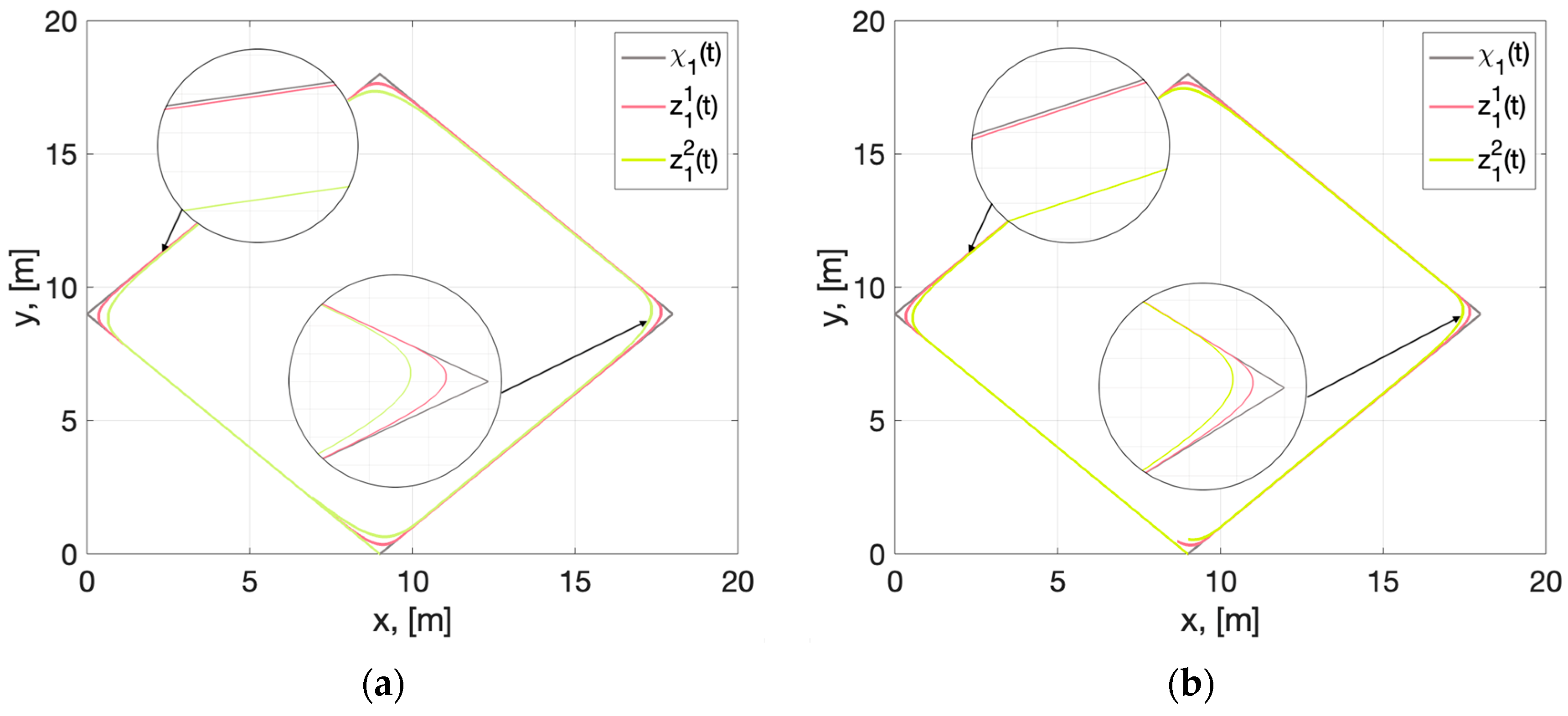
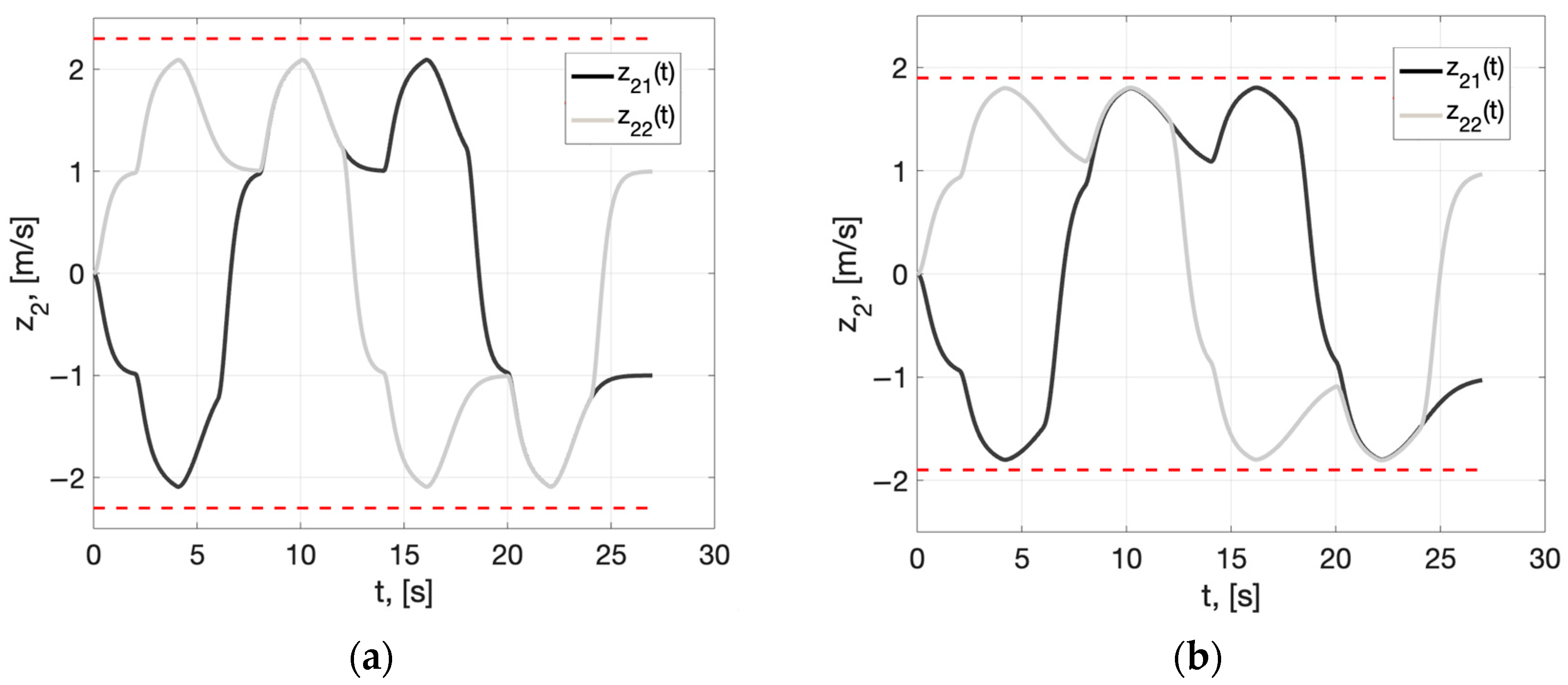
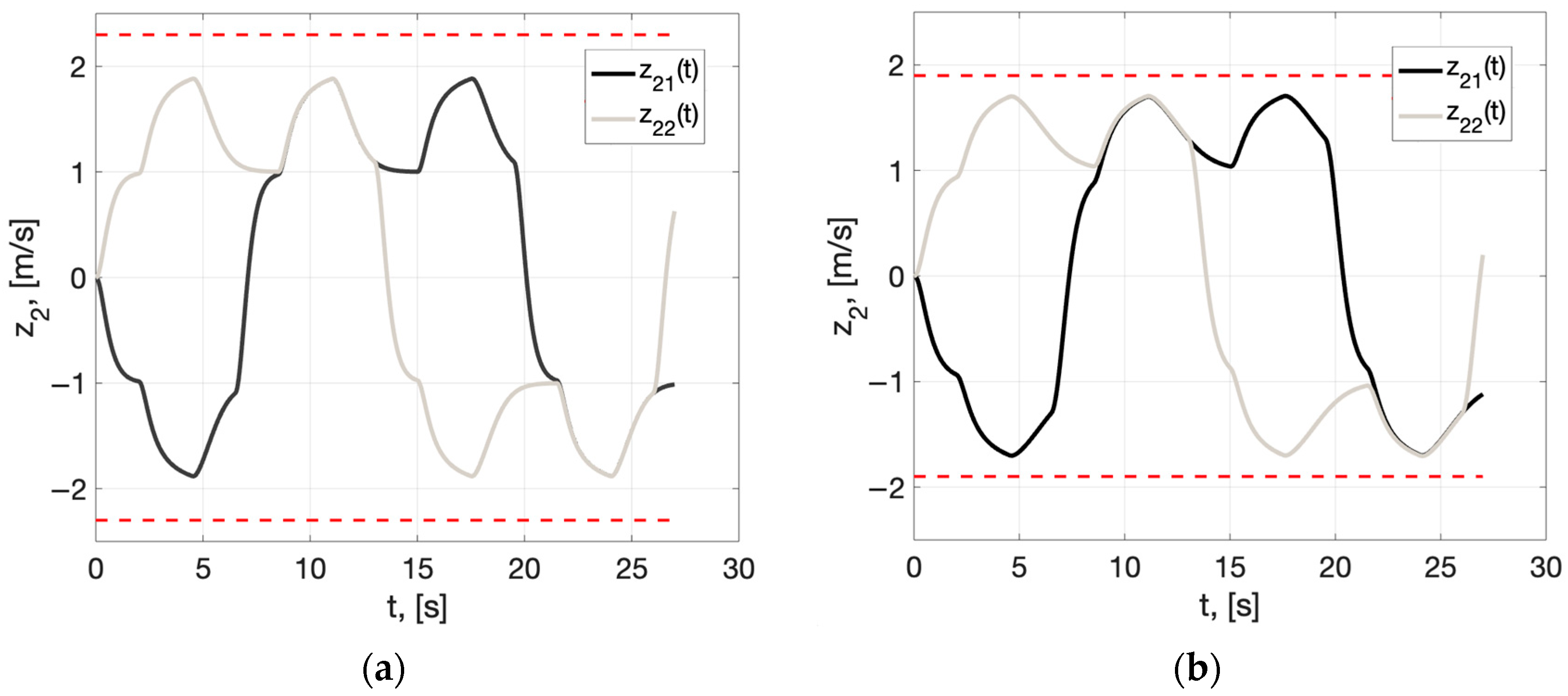
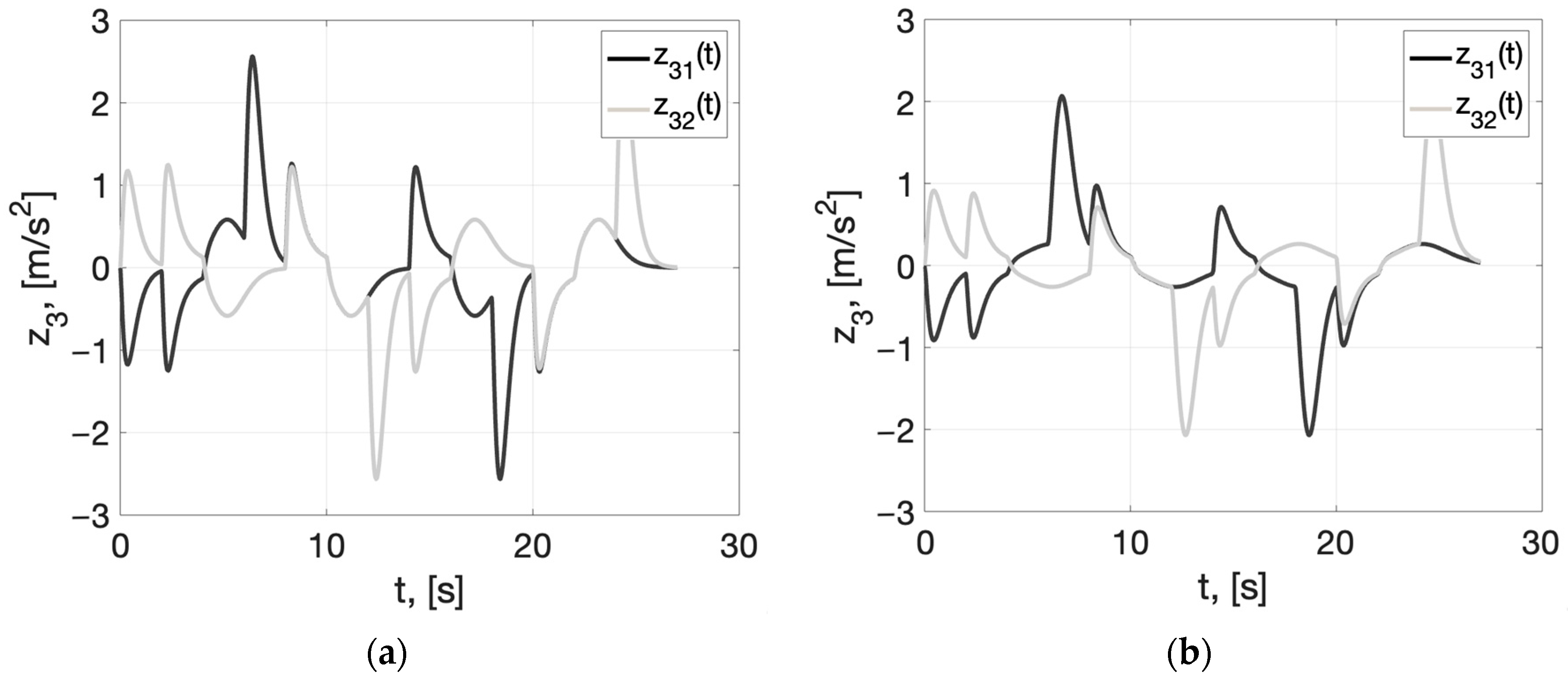
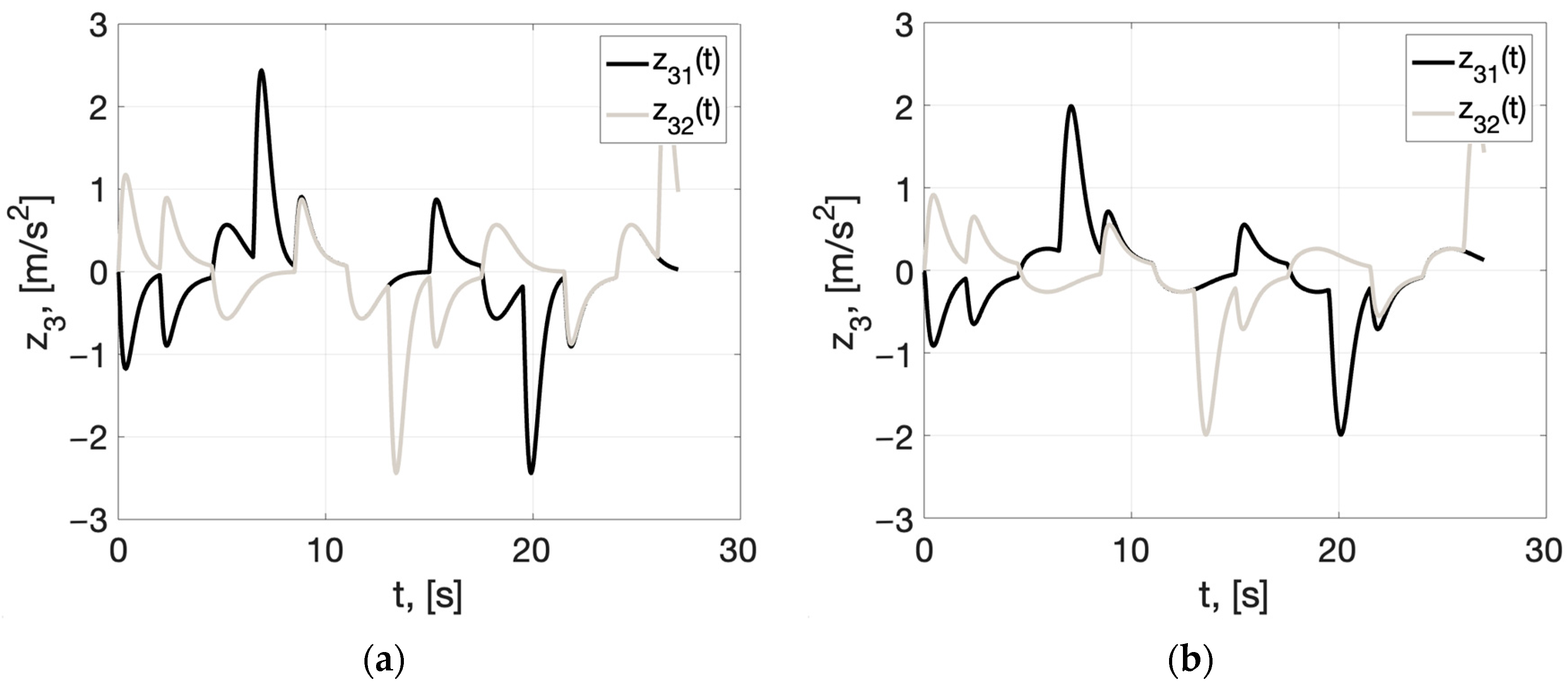
At different nominal values of (4), the signals $z_i(t)$ will automatically approximate the external signals and their derivatives in the neighborhood of special points in different ways. In the steady-state mode, in the admissible cases, their forms will be almost identical. The results of the corresponding numerical simulations are presented in Section 3.

Second, by changing the dimensionality of the tracking differentiator blocks, it is possible to automatically generate smoothed trajectories with defined constraints in phase spaces of different dimensionalities. For example, the system (32) at $\forall z_i\in R$ generates an achievable trajectory for a single-channel control plant (e.g., a single-link manipulator), and at $\forall z_i\in R^3$ it generates a spatial trajectory for a UAV [25].

From a computational viewpoint, the dynamic smoothing algorithm (32) is a sigmoid computation with three integration operations. Their implementation is not difficult using any software. The counting time of the algorithm is negligible and does not lead to lag in real-time operation when vector signals $z_1(t)\approx {\chi }_1(t),$ $z_2(t)\approx {\dot{\chi }}_1(t),$ $z_3(t)\approx {\ddot{\chi }}_1(t),$ and $w(t)\approx {\stackrel{⃛}{\chi }}_1(t)$ are input to the tracking system of the mobile robot as needed.

2.3.3. Reasons for Designing Tracking Differentiators with Different Block Numbers

As was shown in the previous subsection, it is sufficient to apply a dynamic model consisting of three blocks (32) to smooth external signals and to recover their derivatives of the first, second, and even third orders. However, the number of blocks of the tracking differentiator can be both reduced and increased depending on the conditions of the problem to be solved. The main factors influencing the dimensionality of the differentiator are as follows:

• Methods used to design control in a tracking system of a mobile robot;
• The considered dynamic order of the control plant;
• Noisiness/noiselessness of the external signal ${\chi }_1(t).$

For example, to solve the problem of tracking by the output variables $x(t),y(t)$ of System (1) of reference signals under the influence of parametric and external disturbances, we can apply a decomposition method for the design of sigmoid feedback, similar to the method we applied in the previous section for the design of a tracking differentiator [24]. In this method, the first derivatives of the reference influences are treated as external disturbances (as in System (22)), and only the reference influences are used to form the static feedback. Another approach is to use mixed-variable observers in tracking systems [27]. In this case, for feedback design, it is not necessary to obtain separate estimates of the derivatives of the reference influences. Thus, in both approaches, we only need to know the reference signals. If these signals do not contain parasitic disturbances, a single-block tracking differentiator with the minimum possible dynamic order can be used to smooth them:

$${\dot{z}}_1=-p_1\sigma (l_1(z_1-{\chi }_1)),z_1(0)={\chi }_1(0),$$

(33)

where $z_1\in R^2$. The inequalities for the choice of gains $p_1,l_1=\mathrm{const}>0$ considering the constraints on the velocity and acceleration of the mobile robot, similar to (29), (31), are of the form

$$\begin{array}{l}\left[\begin{array}{l}1.25X_1<p_1\le Y_1,\\ p_1^2{l}_1\le Y_2;\end{array}\right.\\ p_1=Y_1,l_1=Y_2/Y_1^2.\end{array}$$

(34)

The shapes of the smoothed curves obtained using the tracking differentiators (32) and (34) under the same constraints (4) will be almost identical.

The signals of the derivatives of the reference influences are usually needed in program control systems [28] as well as when using the feedback linearization method [3]. The order of the required derivatives depends on the number of dynamic links to be considered and is equal to the relative degree of the model used in the control plant.

Let derivatives up to and including $n$-th order be required for the design of the tracking system of a wheeled robot. The tracking differentiator, which smooths the external deterministic signal ${\chi }_1(t)$ and recovers its $n$ derivatives, consists of $(n+1)$ blocks and has a common order $2(n+1)$:

$$\begin{array}{l}{\dot{z}}_i=z_{i+1},i=\overline{1,n};{\dot{z}}_{n+1}=-p_{n+1}\sigma (l_{n+1}{e}_{n+1})=\\ =-p_{n+1}\sigma (l_{n+1}(z_{n+1}+p_n\sigma (l_n(z_n+p_{n-1}\sigma (l_{n-1}(\dots (z_2+p_1\sigma (l_1(z_1-{\chi }_1)))\dots ))))));\\ z_1(0)={\chi }_1(0),z_i(0)=\overrightarrow{0},i=\overline{2,n+1},\end{array}$$

(35)

where $z_i\in R^2,i=\overline{1,n+1}$ are differentiator variables, the vector variable $z_1(t)$ defines the position of the center point of the wheeled platform, and the variable $z_i(t)$ is its $(i-1)$-th derivative, $i=\overline{2,n+1},$ $z_1^{(n+1)}={\dot{z}}_{n+1}.$

To set the tracking differentiator (35), the constraints of a particular mobile robot on the higher derivatives are used. To fulfill the constraints on the state variables of the differentiator, its corrective influences, and their rate of change (i.e., constraints on the robot’s control influences and their rate of change), nominal values $(n+2)$ are required

$$‖y_1^{(i)}‖\le Y_i=\mathrm{const}>0,t\ge 0,Y_i^2<Y_{i+1},i=\overline{1,n+2}.$$

Equations for selection gains of tracking differentiator (35) at which the constraint of its variables is ensured

$$‖z_1^{(i)}‖\le Y_i,t\in [0;T],i=\overline{1,n+2}$$

are similar to the system of dual inequalities (29) and have the following form:

$$\left[\begin{array}{l}2.75/l_2+1.25X_1<p_1\le Y_1-2.2/l_2,\\ 2.75/l_{i+1}+1.25p_{i-1}^2{l}_{i-1}<p_i\le Y_i-2.2/l_{i+1},i=\overline{2,n};\\ 1.25p_n^2{l}_n<p_{n+1}\le Y_{n+1};\\ p_{n+1}^2{l}_{n+1}\le Y_{n+2}.\end{array}\right.$$

(36)

The iterative procedure for setting the gains of sigmoid functions based on the system of inequalities (36) minimizing the steady-state tracking error (30) is similar to (31):

$$\begin{array}{l}{p}_{n+1}=Y_{n+1},l_{n+1}=Y_{n+2}/p_{n+1}^2,\\ p_n=Y_n-2.2/l_{n+1},l_n=(0.8p_{n+1}-{\beta }_n)/p_n^2,\\ p_i=Y_i-2.2/l_{i+1},l_i=(0.8p_{i+1}-{\beta }_i-2.2/l_{i+2})/p_i^2,i=\overline{n-1,1},\end{array}$$

(37)

where ${\beta }_i,i=\overline{1,n}$ are very small positive constants.

Finally, the third factor influencing the choice of the dynamic order of the tracking differentiator is related to the need to filter the external signal if it additively contains parasitic noise ${\overline{\chi }}_1(t)={\chi }_1+\eta (t),$ for example, white noise $\eta (t)$ with zero mathematical expectation and bounded variance.

Note that the noisy signal enters the input of the tracking differentiator (35) and passes through a chain of integrators. Thus, there is natural filtering of the input signal, which improves with increasing number of integrators. Analytical analysis and simulation results have shown that extending the dynamic order of the tracking differentiator is an alternative to installing low-pass prefilters [29]. Two or three integration operations are often sufficient to obtain good performance. For example, if the recovery of the derivatives of the external signal is not a problem, a two or three (32) block tracking differentiator should be used instead of a single-block differentiator (33) for smoothing and filtering the external signal. In turn, instead of a three-block differentiator (32), a four- or five-block tracking differentiator must be used in order to obtain signals of satisfactory quality up to and including the second derivative.

Note that, as in the Kalman filter setting, when selecting gains of sigmoidal functions, we have to compromise between tracking accuracy and filtering features of the tracking differentiator [23]. Therefore, another algorithm is needed instead of the procedure for setting gains $p_i,l_i$ (37). However, a detailed analysis of this problem is beyond the framework of this research.

2.3.4. Some Aspects of Designing Paths and Polygons

The use of tracking differentiators can greatly simplify the computational aspect of planning achievable trajectories offline on a polygon with stationary obstacles.

Let a wheeled robot have a primary operating scenario in the form of a sequence of 3D points defined in a fixed Cartesian coordinate system $Oxy$, considering time

$$(x_i,y_i,t_i),i=\overline{1,m},t_i<t_{i+1},t_1=0;t_m=T.$$

(38)

Connecting all neighboring pairs of point $(x_i,y_i,t_i)$ and $(x_{i+1},y_{i+1},t_{i+1})$ by segments

$$\frac{{\chi }_{11}-x_i}{x_{i+1}-x_i}=\frac{{\chi }_{12}-y_i}{y_{i+1}-y_i}=\frac{t-t_i}{t_{i+1}-t_i},t\in [t_i;t_{i+1}),i=\overline{1,m-1},$$

we obtain a primitive non-smooth 3D trajectory and, accordingly, the primary reference influences for both output variables $x(t),y(t)$ of the system (1):

$$\left\{\begin{array}{l}{\chi }_{11}=\frac{(x_{i+1}-x_i)t+x_i{t}_{i+1}-x_{i+1}{t}_i}{t_{i+1}-t_i},\\ {\chi }_{12}=\frac{(y_{i+1}-y_i)t+y_i{t}_{i+1}-y_{i+1}{t}_i}{t_{i+1}-t_i},t\in [t_i;t_{i+1}),i=\overline{1,m-1}.\end{array}\right.$$

(39)

In standard approaches, special analytical approximations are used to smooth the angles of the composite trajectory (39) [11]. In this case, the problem of ensuring the specified constraints on the velocity and acceleration of the robot requires additional algorithmization. If the singular points are sufficiently numerous, analytical smoothing methods provide a large computational load, which makes it difficult to use them in real time. In addition, composite analytical reference influences take up much memory when stored on the on-board computer.

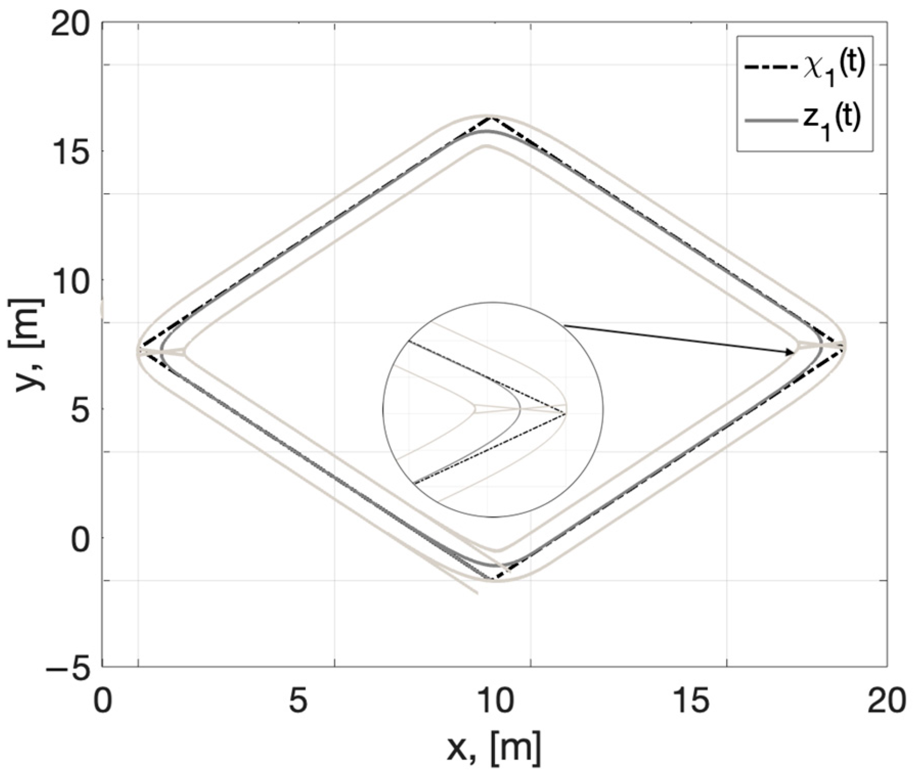
The application of dynamic smoothing algorithms for primitive trajectories (39) completely eliminates these problems. Only a sequence of points (38) is stored in the on-board computer memory, and smoothing of the corresponding primitive trajectories (39) is performed in real time using a tracking differentiator (35), (37) of the required dimensionality.

Note that this method is not intended for solving terminal problems and does not provide an exact fit to the reference points. However, it can be used for offline simulation on a compressed time scale. We can quickly correct the smoothed trajectory obtained after the first run of the algorithm and achieve the desired result by correcting the coordinates of particular points (38). At the same time, visual results will be obtained quickly and without cumbersome analytical calculations. For such a process, it is sufficient to use a single-block tracking differentiator (33).

Let us consider some aspects of planning a safe route for an oversized wheeled vehicle on a polygon with stationary obstacles. The opposite task is to arrange objects on the polygon (factory workshop, warehouse) so that the robot can safely fulfill the operating scenario. Therefore, it is necessary to consider the dimensions of the vehicle when planning the polygon. The developed dynamic smoothing algorithm can be applied to graphically represent the position change not only for the center of mass of the wheeled platform but also for its corner points. In this problem, it is better (but not necessarily) to use a two-block tracking differentiator

$$\begin{array}{l}{\dot{z}}_1=z_2,{\dot{z}}_2=-p_2\sigma (l_2(z_2+p_1\sigma (l_1(z_1-{\chi }_1)))),\\ z_{1,2}\in R^2,z_1(0)={\chi }_1(0),z_2(0)=\overrightarrow{0}.\end{array}$$

(40)

Its parameters are determined from the procedure (37) at $n=1$ and have the form:

$$\begin{array}{l}{p}_2=Y_2,l_2=Y_3/p_2^2=Y_3/Y_2^2,\\ p_1=Y_1-2.2/l_2=Y_1-2.2Y_2^2/Y_3\\ l_1=(0.8p_2-{\beta }_1)/p_1^2=(0.8Y_2-{\beta }_1)/{[Y_1-2.2Y_2^2/Y_3]}^2.\end{array}$$

(41)

Let us present the corresponding computations for a symmetrical rectangular wheeled platform whose center of mass is located at the intersection of diagonals in the middle of the center line. Let us introduce the following notations: $\rho >0$ is the distance (with a small margin) from the center of mass to each corner point of the platform; $\alpha <\pi /2$ is the value of the angle between the center line of the platform and its diagonals; $(z_{11}(t);z_{12}(t))$ is the current coordinates of the center of mass of the platform; and $({\overline{z}}_{11,j}(t);{\overline{z}}_{12,j}(t))$ is the current coordinates of the corner points of the platform, $j=\overline{1,4}.$ Recall that in System (1), $\theta$ is the angle between the $Ox$ axis and the center line of the platform, which coincides with the direction of the velocity vector, $\theta =\mathrm{arct}g({\dot{y}}_{12}/{\dot{y}}_{11})$ (3).

First, the waypoints of the mobile robot (38) are planned on the polygon. The primary reference influences (39) are entered into the input of the tracking differentiator (41) with the output variables $z_{11}(t),z_{12}(t)$, which simulate the position of the platform’s center of mass in the stationary Cartesian coordinate system. The formulas for computing the current coordinates of the platform corner points are as follows

$$\begin{array}{l}\left\{\begin{array}{l}{\overline{z}}_{11,1}(t)=z_{11}(t)+\rho \cos (\overline{\theta }(t)+\alpha ),\\ {\overline{z}}_{12,1}(t)=z_{12}(t)+\rho \sin (\overline{\theta }(t)+\alpha );\end{array}\right.\left\{\begin{array}{l}{\overline{z}}_{11,2}(t)=z_{11}(t)+\rho \cos (\overline{\theta }(t)-\alpha ),\\ {\overline{z}}_{12,2}(t)=z_{12}(t)+\rho \sin (\overline{\theta }(t)-\alpha );\end{array}\right.\\ \left\{\begin{array}{l}{\overline{z}}_{11,3}(t)=z_{11}(t)+\rho \cos (\overline{\theta }(t)+\alpha +\pi ),\\ {\overline{z}}_{12,3}(t)=z_{12}(t)+\rho \sin (\overline{\theta }(t)+\alpha +\pi );\end{array}\right.\left\{\begin{array}{l}{\overline{z}}_{11,4}(t)=z_{11}(t)+\rho \cos (\overline{\theta }(t)-\alpha -\pi ),\\ {\overline{z}}_{12,4}(t)=z_{12}(t)+\rho \sin (\overline{\theta }(t)-\alpha -\pi );\end{array}\right.\\ \overline{\theta }(t)=\mathrm{arct}g(z_{22}(t)/z_{21}(t))\end{array}$$

(42)

and are correct at $0\le \overline{\theta }\le \pi /2$. Technically, at other directions of the velocity vector, we should change the signs $\pm$ in Equation (42) and use additional logic. Let us not complicate the algorithm and track the direction of motion of the platform. 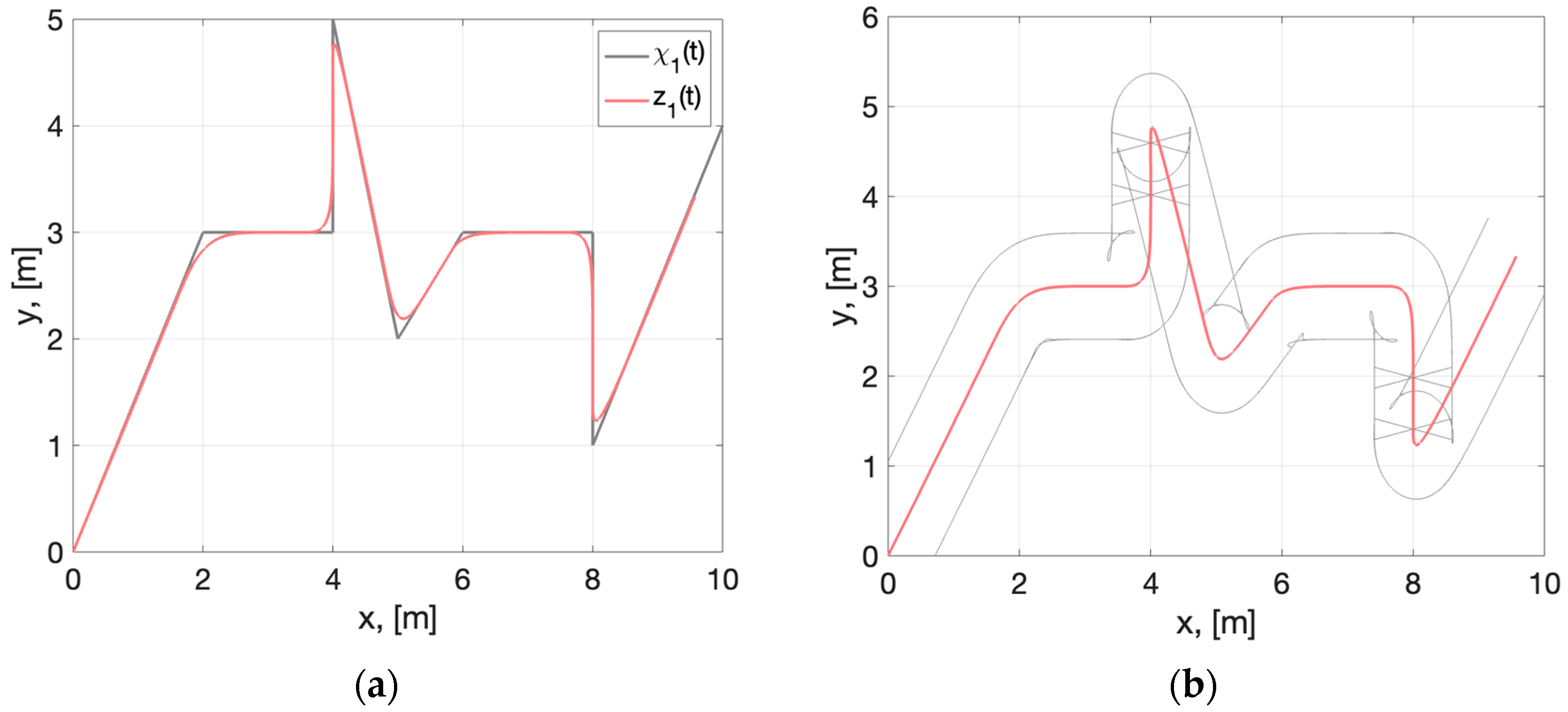When changing the quadrant in which the angle $\overline{\theta }$ is located, the angular points on the right side ${\overline{z}}_{12}(t),{\overline{z}}_{13}(t)$ will represent the path of the points on the left side ${\overline{z}}_{11}(t),{\overline{z}}_{14}(t)$ and conversely. Thus, curves $(z_{11}(t),z_{12}(t))$ and (42) shown on the same plot will indicate the dimensional footprint of the wheeled platform, which is required.

Such representations are a visual and convenient tool for polygon design, object placement, and trajectory planning.

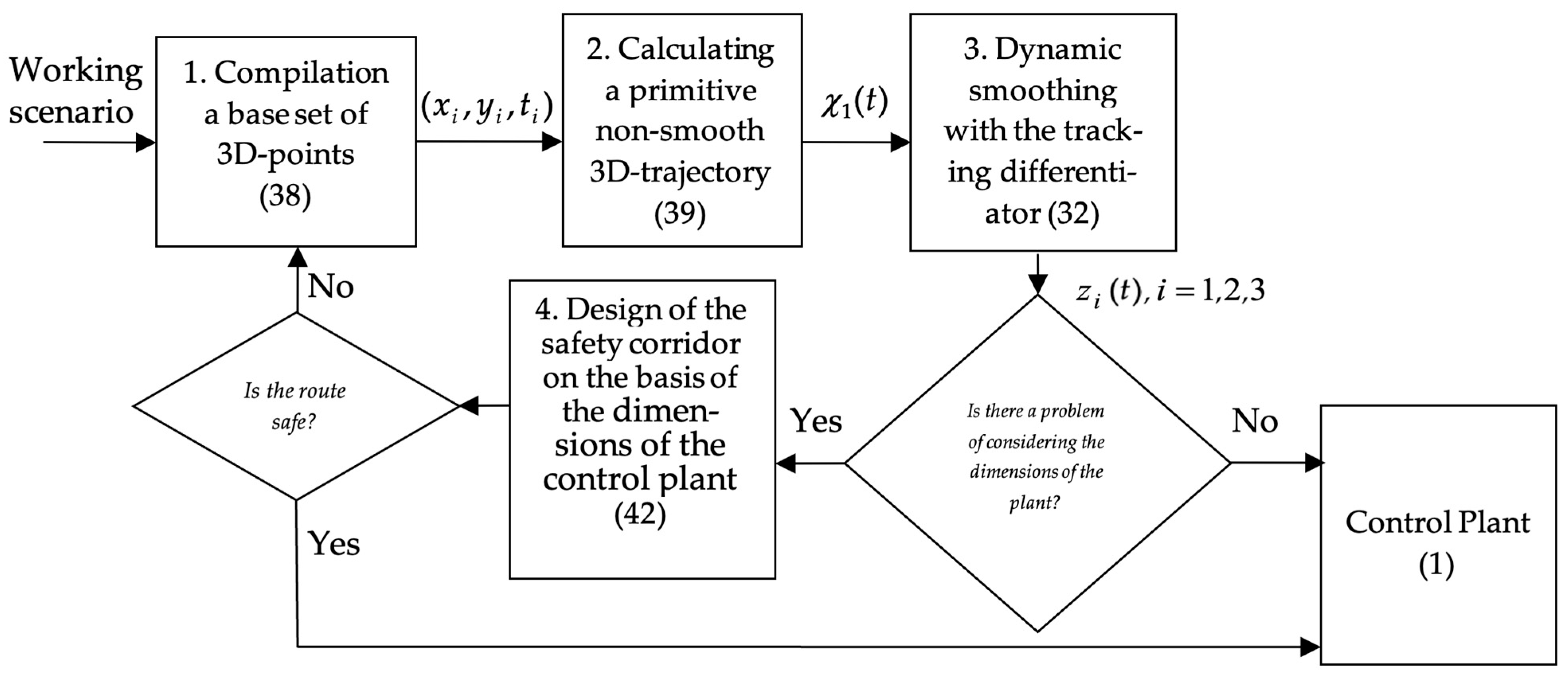
The developed algorithms complex is a convenient tool for mobile robot motion planning and polygon design. Figure 1 shows a flowchart of the robot motion planning process on a polygon with stationary obstacles.

This process includes the following:

• Designing a base set of 3D points (38) for a specific workspace considering obstacles, robot velocity and turning radius constraints, route length, etc.;
• Computing a primitive non-smooth trajectory (39) over a reference set of 3D points (38);
• Smoothing of the primitive trajectory using a tracking differentiator. This process is a numerical solution of differential Equation (32), i.e., calculation of the sigmoid and integration operations;
• Dimension trajectory simulation and safe corridor visualization (42).

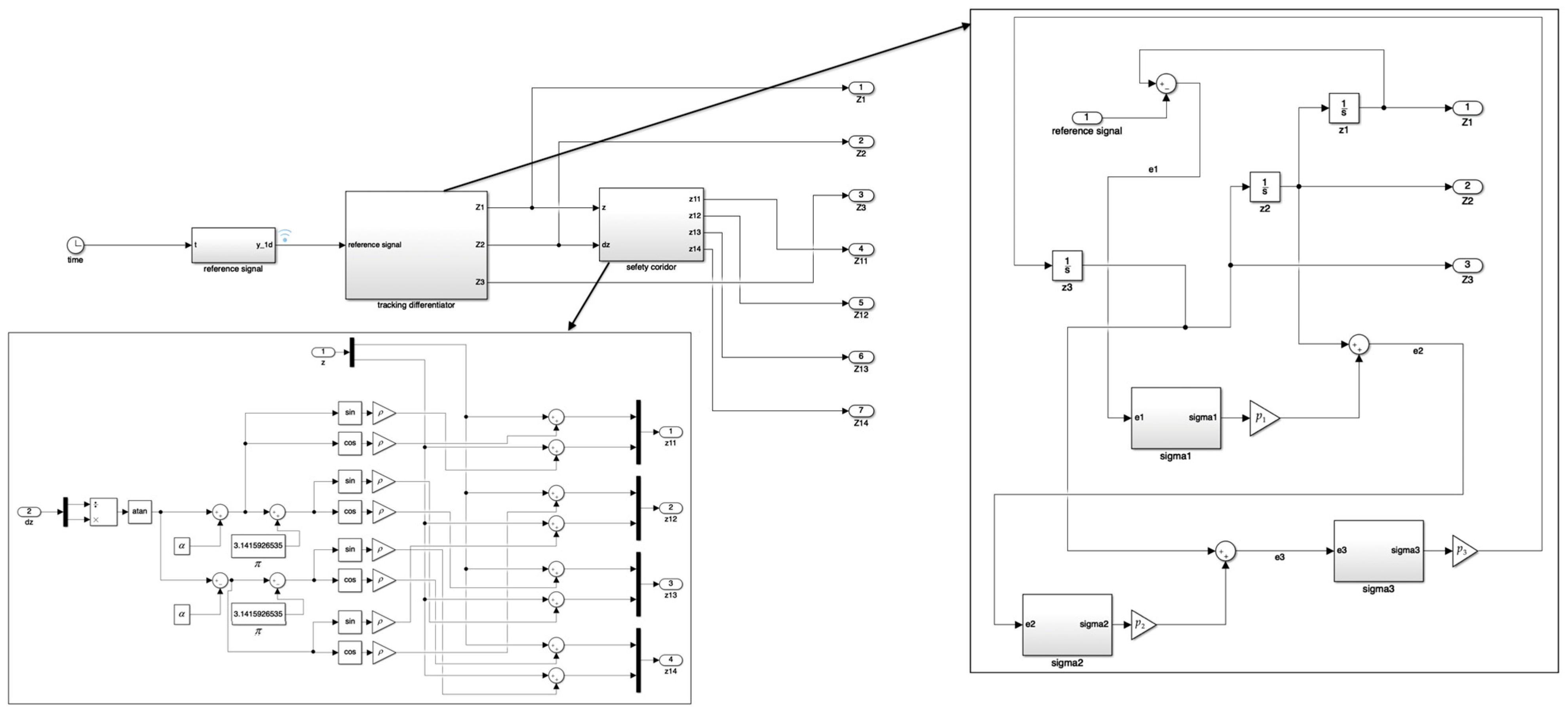
Appendix A presents a structural diagram created by simulating the algorithms developed in the MATLAB Simulink software environment. The main interface of Simulink is a graphical block diagraming tool and a customizable set of block libraries. Therefore, the structure of the graphical block diagram in the MATLAB Simulink software environment (Figure A1) is similar to that of the flowchart shown in Figure 1. At the same time, Figure A1 clearly demonstrates the computational process and the computational operations performed.

Note that in the first stage, machine learning methods can be effectively used to generate primitive trajectories considering various criteria [30]. The result is the solution of discrete optimization problems in the form of a set of discrete waypoints. As mentioned, designing a smooth and achievable trajectory on their basis requires additional tools [16].

In the next subsection, the results of numerical simulations of this and other developed algorithms will be presented.

3. Results

To verify the developed algorithms, simulation modeling in the MATLAB Simulink environment was carried out. We used the Euler method with a constant step of ${10}^{-2}$ for numerical integration. The results of two experiments using a three-block tracking differentiator (32) are presented below. The first experiment demonstrates the smoothing processes of primitive trajectories for the robot’s center of mass under different sets of constraints (4). In the second experiment, for one of the smoothed trajectories, a motion trajectory is simulated considering the vehicle dimensions.

In the first experiment, the design constraints of two civilian wheeled robots moving in an urban environment were used to set the gains of the tracking differentiator. Based on the inequalities (29), the following gains of the tracking differentiator (32) were adopted for the first robot with a velocity of up to 2.3 m/s:

$$p_1=2.3, l_1=1.4, p_2=20, l_2=0.5, p_3=250, l_3=0.3.$$

(43)

For the second robot with a developing velocity of up to 1.9 m/s, the following gains of the tracking differentiator (32) were adopted:

$$p_1=1.9, l_1=1.4, p_2=16, l_2=0.5, p_3=160, l_3=0.3.$$

(44)

The robots’ motion was planned along a rhombus defined in a fixed Cartesian coordinate system. Thirteen waypoints $(x_i,y_i)$ were randomly marked on the sides of the rhombus. Based on them, we generated two sets of 3D waypoint sequences $(x_i, y_i, t_i),$ $i=\overline{1,13}$ (38), which differ only in the values of time $t_i$, by which the average velocity of motion on each path segment is defined and limited. In the first sequence, the maximum velocity was limited by $2.5 \mathrm{m}/\mathrm{s}$ and in the second by $2 \mathrm{m}/\mathrm{s}$. We purposely used values slightly higher than the above-mentioned robot velocities.

Joining neighboring pairs of points by segments, we obtain two primitive non-smooth 3D trajectories (39): for the first sequence at $v_{\max }=2.5 \mathrm{m}/\mathrm{s}$ in the form of

$$\begin{array}{l}{\chi }_{11}=-t+9,{\chi }_{12}=t,t\in [0;2);\\ {\chi }_{11}=-2.5t+12,{\chi }_{12}=2.5t-3,t\in [2;4);\\ {\chi }_{11}=-t+6,{\chi }_{12}=t+3,t\in [4;6);\\ {\chi }_{11}=t-6,{\chi }_{12}=t+3,t\in [6;8);\\ {\chi }_{11}=2.5t-18,{\chi }_{12}=2.5t-9,t\in [8;10);\\ {\chi }_{11}=t-3,{\chi }_{12}=t+6,t\in [10;12);\\ {\chi }_{11}=t-3,{\chi }_{12}=-t+30,t\in [12;14);\\ {\chi }_{11}=2.5t-24,{\chi }_{12}=-2.5t+51,t\in [14;16);\\ {\chi }_{11}=t,{\chi }_{12}=-t+27,t\in [16;18);\\ {\chi }_{11}=-t+36,{\chi }_{12}=-t+27,t\in [18;20);\\ {\chi }_{11}=-2.5t+66,{\chi }_{12}=-t+24,t\in [20;22);\\ {\chi }_{11}=-t+33,{\chi }_{12}=-t+24,t\in [22;24);\\ {\chi }_{11}=-t+33,{\chi }_{12}=t-24,t\ge 24,{\chi }_{ij}[m],t[s];\end{array}$$

(45)

for the second sequence at $v_{\max }=2\mathrm{m}/\mathrm{s}$ in the form of

$$\begin{array}{l}{\chi }_{11}=-t+9,{\chi }_{12}=t,t\in [0;2);\\ {\chi }_{11}=-2t+11,{\chi }_{12}=2t-2,t\in [2;4.5);\\ {\chi }_{11}=-t+6.5,{\chi }_{12}=t+2.5,t\in [4.5;6.5);\\ {\chi }_{11}=t-6.5,{\chi }_{12}=t+2.5,t\in [6.5;8.5);\\ {\chi }_{11}=2t-15,{\chi }_{12}=2t-6,t\in [8.5;11);\\ {\chi }_{11}=t-4,{\chi }_{12}=t+5,t\in [11;13);\\ {\chi }_{11}=t-4,{\chi }_{12}=-t+31,t\in [13;15);\\ {\chi }_{11}=2t-19,{\chi }_{12}=-2t+46,t\in [15;17.5);\\ {\chi }_{11}=t-1.5,{\chi }_{12}=-t+28.5,t\in [17.5;19.5);\\ {\chi }_{11}=-t+37.5,{\chi }_{12}=-t+28.5,t\in [19.5;21.5);\\ {\chi }_{11}=-2t+59,{\chi }_{12}=-2t+50,t\in [21.5;24);\\ {\chi }_{11}=-t+35,{\chi }_{12}=-t+26,t\in [24;26);\\ {\chi }_{11}=-t+35,{\chi }_{12}=t-26,t\ge 26,{\chi }_{ij}[m],t[s].\end{array}$$

(46)

In order to ensure zero initial conditions of the uncertainty (24) based on $z_1(0)={\chi }_1(0),$ $z_i(0)=\overrightarrow{0},i=2,3$ considering (45), (46), the same initial conditions were set in the tracking differentiators (32), (43) and (32), (44) to ensure zero initial conditions

$$z_1(0)=(9;0),z_2(0)=(0;0),z_3(0)=(0;0).$$

The simulation results of both tracking differentiators with both primary trajectories are shown below. Figure 2 shows plots of the reference rhombus $({\chi }_{11}(t),{\chi }_{12}(t))$ and output variables $(z_{11}(t),z_{12}(t))$ of the differentiators (32), (43) and (32), (44) for tracking trajectories (45) (Figure 2a) and (46) (Figure 2b). Further, the left figures (a) show the simulation results of the tracking differentiator (32), (43); the right figures (b) show the simulation results of the tracking differentiator (32), (44). Figure 3 and Figure 4 show plots of the first derivatives of $z_{21}(t),z_{22}(t)$, simulating velocities, when trajectories (45) and (46) are tracked, and velocity constraints corresponding to the tracking differentiators (32), (43) and (32), (44). Figure 5 and Figure 6 show plots of the second derivatives of $z_{31}(t),z_{32}(t)$, simulating accelerations, when trajectories (45) and (46) are tracked, correspondingly.

The plots of Figure 1 show that the tracking differentiators with different gains effectively smooth the angles of the rhombus of the primitive trajectories (45), (46), set with different values of velocities of motion. At the same time, the tracking differentiator (32), (44), set with a velocity limit of 1.9 m/s ($1.9<2,$ $1.9<2,5$), provides a larger (compared to the tracking differentiator (32), (43)) tracking error $e_1(t)=z_1(t)-{\chi }_1(t)$ both at singular points and in the steady state. Thus, the quality of angle smoothing deteriorates if the maximum velocity of the primitive trajectory exceeds the maximum velocity $Y_1$ assumed at the setting of the tracking differentiator.

The plots of Figure 3 and Figure 4 show that the first derivatives of the smoothed trajectories $z_{21}(t),z_{22}(t)$ in all cases do not exceed the design velocity constraints. The second derivatives of $z_{31}(t),z_{32}(t)$ are constrained (Figure 5 and Figure 6).

It can be concluded that the tracking differentiator provides good performance and provides velocity and acceleration constraints for tracking different trajectories. By reducing the velocity near singular points at the planning stage, the smoothing quality of primitive trajectories and their derivatives can be controlled.

In the second experiment, the dimensions of the wheeled robot “SRX 1” were adopted to model the safety corridor: 765 × 1370 mm (width × length). Figure 7 shows plots of the output variables $(z_{11}(t),z_{12}(t))$ of the differentiator (32), (44), tracking primitive trajectory (46), and the trajectories of the platform angular points (42).

As can be seen from Figure 7, when changing the direction of motion, the trajectories of the angular points of the right and left sides change places, but this does not change the shape of the dimensional trajectory.

Figure 8 shows the results of smoothing (Figure 8a) and generating a dimensional trajectory (Figure 8b) for a more complex route specified by the following set of 3D points:

$$\begin{array}{l}(x_i[m],y_i[m],t_i[s]):(0,0,0);(2,3,3);(4,3,6);(4,5,9);\\ (5,2,12);(6,3,15);(8,3,18);(8,1,21);(10,4,24).\end{array}$$

(47)

Based on these data, a non-smooth 3D trajectory ${\chi }_1(t)={({\chi }_{11}(t),{\chi }_{12}(t))}^{\mathrm{T}}$ (39) was generated for simulation. It is also presented in Figure 8a.

4. Discussion

The dynamic smoothing method (32) for primitive trajectories is the main result of this research. An explicit comparison of its computational complexity with analytical smoothing methods, which were described in the introduction, is rather difficult because these methods are fundamentally different from each other. The classical methods [11,12,13,14,15,16] result in a complete analytical description of the reference trajectory (it is an approximation of a specified set of waypoints). Computational complexity is directly proportional to the number of reference points and fragments with different boundary conditions. For each fragment of the trajectory, it is necessary to calculate the coefficients of the polynomial and control to fulfill the constraints. In addition, each new sequence of points requires an individual organization of calculations.

The method of dynamic smoothing of reference trajectories as a vector signal generates the tracking differentiator (32). The gains of the differentiator are set immediately (31) and do not change while processing different sequences of points for the same robot. The smoothing process is a numerical solution of the differential Equation (32). Complicating the shape of the reference curve does not lead to a more complex algorithm and increased computational operations necessary to smooth. If a set of waypoints considering time (38) is specified, they are automatically connected by segments (39) before being input to the differentiator. If a non-smooth reference signal is applied to the input of the tracking differentiator, it will be automatically smoothed without additional calculations.

In this paper, we present only the results of numerical experiments. However, the simulation was organized in such a way that the reference signal was applied to the system in real time using the “clock” block, which is named on the Figure A1 as the “time” block (see Appendix A).

It can be concluded that the complex use of machine learning methods (in the first stage) and the developed dynamic smoothing method (in the second stage) will allow full automation of the process of planning achievable trajectories. This is a prerequisite for the design of autonomous unmanned vehicles.

5. Conclusions

To provide a complete design of an automatic motion control system for a mobile robot, a universal dynamic smoothing method is proposed in this paper. It automatically generates a smooth curve that satisfies the design constraints of a particular robot for velocity and acceleration at any number of reference points. As a result of using a higher-order tracking differentiator with continuous correction, the state variables of the differentiator generate a smooth reference signal and its derivative, which are used in the feedback loop by the real control plant.

In future research, it is planned to develop the algorithm for considering the dimensions of the control plants under consideration, considering the obstacles present in the course of movement along the developed route. However, at the moment, the dimensions of the control plants are already considered on the basis of the obtained data using the tracking differentiator (32) with the computationally simple algorithm (42). This is also an effective tool for trajectory planning, considering the objects and obstacles present on the polygon.

References

1. Chu, X.; Peng, Z.; Wen, G.; Rahmani, A. Distributed Fixed-Time Formation Tracking of Multi-Robot Systems with Nonholonomic Constraints. Neurocomputing 2018, 313, 167–174. [Google Scholar] [CrossRef]
2. Trojnacki, M.; Dąbek, P. Mechanical Properties of Modern Wheeled Mobile Robots. JAMRIS 2019, 13, 3–13. [Google Scholar] [CrossRef]
3. Pesterev, A.V.; Rapoport, L.B.; Tkachev, S.B. Canonical Representation of a Nonstationary Path Following Problem. J. Comput. Syst. Sci. Int. 2015, 54, 656–670. [Google Scholar] [CrossRef]
4. Kochetkov, S.A. Mobile Robot Trajectory Control under Influence of Unknown Perturbation. MESA 2019, 10, 725–732. [Google Scholar]
5. Tzafestas, S.G. Mobile robot control and navigation: A global overview. J. Intell. Robot. Syst. 2018, 91, 35–58. [Google Scholar] [CrossRef]
6. Zhou, C.; Huang, B.; Fränti, P. A Review of Motion Planning Algorithms for Intelligent Robots. J. Intell. Manuf. 2022, 33, 387–424. [Google Scholar] [CrossRef]
7. Debnath, S.K.; Omar, R.; Latip, N.B.A.; Shelyna, S.; Nadira, E.; Melor, C.; Chakraborty, T.K.; Natarajan, E. A Review on Graph Search Algorithms for Optimal Energy Efficient Path Planning for an Unmanned Air Vehicle. Indones. J. Electr. Eng. Comput. Sci. 2019, 15, 743–749. [Google Scholar] [CrossRef]
8. Kang, J.G.; Lim, D.W.; Choi, Y.S.; Jang, W.J.; Jung, J.W. Improved RRT-connect Algorithm Based on Triangular Inequality for Robot Path Planning. Sensors 2021, 21, 333. [Google Scholar] [CrossRef]
9. Lin, Z.; Yue, M.; Chen, G.; Sun, J. Path Planning of Mobile Robot with PSO-based APF and Fuzzy-based DWA Subject to Moving Obstacles. Trans. Inst. Meas. Control 2022, 44, 121–132. [Google Scholar] [CrossRef]
10. Xiang, D.; Lin, H.; Ouyang, J.; Huang, D. Combined improved A* and greedy algorithm for path planning of multi-objective mobile robot. Sci. Rep. 2022, 12, 13273. [Google Scholar] [CrossRef]
11. González, D.; Perez, J.; Milanés, V.; Nashashibi, F. A review of motion planning techniques for automated vehicles. IEEE Trans. Intell. Transpor. Syst. 2015, 17, 1135–1145. [Google Scholar] [CrossRef]
12. Mercy, T.; Van Parys, R.; Pipeleers, G. Spline-Based Motion Planning for Autonomous Guided Vehicles in a Dynamic Environment. IEEE Trans. Control Syst. Technol. 2017, 26, 2182–2189. [Google Scholar] [CrossRef]
13. Lambert, E.; Romano, R.; Watling, D. Optimal Path Planning with Clothoid Curves for Passenger Comfort. In Proceedings of the 5th International Conference on Vehicle Technology and Intelligent Transport Systems, Heraklion, Crete, Greece, 3–5 May 2019; pp. 609–615. [Google Scholar] [CrossRef]
14. Rosu, H.C.; Mancas, S.C.; Hsieh, C.-C. Generalized Cornu-type spirals and their Darboux parametric deformations. Phys. Lett. A 2019, 383, 2692–2697. [Google Scholar] [CrossRef]
15. Cong, D.; Liang, C.; Gong, Q.; Yang, X.; Liu, J. Path planning and following of omnidirectional mobile robot based on B-spline. In Proceedings of the 2018 Chinese Control and Decision Conference (CCDC), Shenyang, China, 9–11 June 2018; IEEE: Piscataway, NJ, USA, 2018; pp. 4931–4936. [Google Scholar] [CrossRef]
16. Sun, Y.; Yang, J.; Zhao, D.; Shu, Y.; Zhang, Z.; Wang, S. A Global Trajectory Planning Framework Based on Minimizing the Risk Index. Actuators 2023, 12, 270. [Google Scholar] [CrossRef]
17. Han, J. Mobile robot path planning with surrounding point set and path improvement. Appl. Soft Comput. 2017, 57, 35–47. [Google Scholar] [CrossRef]
18. Busurin, V.I.; Kazaryan, A.V.; Shtek, S.G.; Zheglov, M.A.; Vasetskiy, S.O.; Kyi, P.L. Frame Micro-Optoelectromechanical Angular Velocity Transducer with Optical Readout Units Based on the Optical Tunneling Effect. Meas. Technol. 2022, 65, 360–365. [Google Scholar] [CrossRef]
19. Bu, X.W.; Wu, X.Y.; Zhang, R.; Ma, Z.; Huang, J. Tracking Differentiator Design for the Robust Backstepping Control of Flexible Air-breathing Hypersonic Vehicle. J. Frankl. Inst. 2015, 352, 1739–1765. [Google Scholar] [CrossRef]
20. Ibraheem, I.K.; Abdul-Adheem, W.R. On the Improved Nonlinear Tracking Differentiator based Nonlinear PID Controller Design. Int. J. Adv. Comput. Sci. Appl. 2016, 7, 234–241. [Google Scholar] [CrossRef]
21. Xie, Y.; Zhang, H.; She, L.; Xiao, G.; Zhai, C.; Pan, T. Design and Implementation of an Efficient Tracking Differentiator. IEEE Access 2019, 7, 101941–101949. [Google Scholar] [CrossRef]
22. Lv, Z.; Jin, S.; Xiong, X.; Yu, J. A New Quick-Response Sliding Mode Tracking Differentiator With its Chattering-Free Discrete-Time Implementation. IEEE Access 2019, 7, 130236–130245. [Google Scholar] [CrossRef]
23. Gao, Y.; Tian, D.; Wang, Y. Fuzzy Self-Tuning Tracking Differentiator for Motion Measurement Sensors and Application in Wide-Bandwidth High-Accuracy Servo Control. Sensors 2020, 20, 948. [Google Scholar] [CrossRef] [PubMed]
24. Antipov, A.S.; Krasnova, S.A.; Utkin, V.A. Synthesis of Invariant Nonlinear Single-Channel Sigmoid Feedback Tracking Systems Ensuring Given Tracking Accuracy. Autom. Remote Control 2022, 83, 32–53. [Google Scholar] [CrossRef]
25. Krasnova, S.A.; Kokunko, Y.G.; Utkin, V.A. Dynamic Models with Sigmoid Corrections to Generation of an Achievable 4D-Trajectory for a UAV and Estimating Wind Disturbances. Electronics 2023, 12, 2280. [Google Scholar] [CrossRef]
26. Belinskaya, Y.S.; Chetverikov, V.N. Covering method for point-to-point control of constrained flat system. IFAC-Pap. OnLine 2015, 48, 924–929. [Google Scholar] [CrossRef]
27. Wang, H.; Zhang, Z.; Tang, X.; Zhao, Z.; Yan, Y. Continuous output feedback sliding mode control for underactuated flexible-joint robot. J. Frankl. Inst. 2022, 359, 7847–7865. [Google Scholar] [CrossRef]
28. Zubova, S.P.; Raetskaya, E.V. Construction of controls providing the desired output of the linear stationary dynamic system. Autom. Remote Control 2018, 79, 775–792. [Google Scholar] [CrossRef]
29. Astolfi, D.; Zaccarian, L.; Jungers, M. On the use of low-pass filters in high-gain observers. Syst. Control Lett. 2021, 148, 104856. [Google Scholar] [CrossRef]
30. Arulkumaran, K.; Deisenroth, M.P.; Brundage, M.; Bharath, A.A. Deep reinforcement learning: A brief survey. IEEE Signal Process. Mag. 2017, 34, 26–38. [Google Scholar] [CrossRef]
Figure 1. Flowchart of the trajectory planning process.
Algorithms 16 00405 g001
Figure 2. Plots of outputs of tracking differentiators z 1 1 ( t ) (32), (43) and z 1 2 ( t ) (32), (44) tracking primitive trajectories χ 1 ( t ) . In (a), for the primitive trajectory (45). In (b), for the primitive trajectory (46).
Algorithms 16 00405 g002
Figure 3. Plots of velocities z 21 ( t ) , z 22 ( t ) of smoothed trajectory (45). In (a), for the tracking differentiator (32), (43). In (b), for the tracking differentiator (32), (44).
Algorithms 16 00405 g003
Figure 4. Plots of velocities z 21 ( t ) , z 22 ( t ) of smoothed trajectory (46). In (a), for the tracking differentiator (32), (43). In (b), for the tracking differentiator (32), (44).
Algorithms 16 00405 g004
Figure 5. Plots of accelerations z 31 ( t ) , z 32 ( t ) of smoothed trajectory (45). In (a), for the tracking differentiator (32), (43). In (b), for the tracking differentiator (32), (44).
Algorithms 16 00405 g005
Figure 6. Plots of accelerations z 31 ( t ) , z 32 ( t ) of smoothed trajectory (46). In (a), for the tracking differentiator (32), (43). In (b), for the tracking differentiator (32), (44).
Algorithms 16 00405 g006
Figure 7. Trajectory considering the dimensions of the wheeled platform.
Algorithms 16 00405 g007
Figure 8. In (a), plots of the output variables ( z 11 ( t ) , z 12 ( t ) ) of the differentiator (32), (44), tracking primitive trajectory (47). In (b), the trajectories of the platform angular points (42).
Algorithms 16 00405 g008
Disclaimer/Publisher’s Note: The statements, opinions and data contained in all publications are solely those of the individual author(s) and contributor(s) and not of MDPI and/or the editor(s). MDPI and/or the editor(s) disclaim responsibility for any injury to people or property resulting from any ideas, methods, instructions or products referred to in the content.