Balancing Project Schedule, Cost, and Value under Uncertainty: A Reinforcement Learning Approach

Abstract

Industrial projects are plagued by uncertainties, often resulting in both time and cost overruns. This research introduces an innovative approach, employing Reinforcement Learning (RL), to address three distinct project management challenges within a setting of uncertain activity durations. The primary objective is to identify stable baseline schedules. The first challenge encompasses the multimode lean project management problem, wherein the goal is to maximize a project’s value function while adhering to both due date and budget chance constraints. The second challenge involves the chance-constrained critical chain buffer management problem in a multimode context. Here, the aim is to minimize the project delivery date while considering resource constraints and duration-chance constraints. The third challenge revolves around striking a balance between the project value and its net present value (NPV) within a resource-constrained multimode environment. To tackle these three challenges, we devised mathematical programming models, some of which were solved optimally. Additionally, we developed competitive RL-based algorithms and verified their performance against established benchmarks. Our RL algorithms consistently generated schedules that compared favorably with the benchmarks, leading to higher project values and NPVs and shorter schedules while staying within the stakeholders’ risk thresholds. The potential beneficiaries of this research are project managers and decision-makers who can use this approach to generate an efficient frontier of optimal project plans.

1. Introduction

Uncertainty is a common challenge in project management and scheduling, which causes many projects to go over budget and miss their deadlines [1]. According to a report that analyzed over 50,000 projects from 1000 organizations, more than half of the projects (56%) had cost overruns, and 60% of them were delayed [2]. According to a 2021 publication by the Project Management Institute, projects worldwide exceed their budget and schedule by 38% and 45%, respectively [3]. The same report also reveals that the products or services delivered by the projects failed to meet the expectations of 44% of customers, implying that the projects did not provide the value that customers anticipated. This situation has prompted researchers in recent years to develop new frameworks for project management that can better deliver value and handle uncertainty.

This paper addresses three new problems in project management and scheduling. The problems account for uncertainty by using stochastic activity durations and are formulated as chance-constrained mixed integer programs (MIPs). The problems also use a multimode setting, where each activity has one or more modes or options from which to choose. Therefore, the solution to the problem involves selecting one mode for each activity.

The first challenge that this study tackles is a new application of Lean Project Management (LPM), which is a widely used framework to deal with the issue of schedule and cost overruns. The aim of LPM is to maximize value (also referred to as benefit in the literature) and minimize waste in the shortest possible time.

The value of a project is determined by a set of attributes that vary according to stakeholders’ preferences. These attributes may include aspects such as design aesthetics, features, functions, reliability, size, speed, availability, and so on [4]. We follow the approach proposed in [5], which defines an objective function that captures the value from the perspective of the customers and stakeholders. In Section 6, we offer an example of how to compute the value of a project.

We present a new LPM approach that can handle uncertain activity durations. Unlike previous studies on project scheduling that did not consider project value, we aim to maximize the value of the project while avoiding cost and schedule overruns. We use reinforcement learning (RL) algorithms to generate a stable project plan that meets the desired threshold for schedule and budget violation probabilities.

We present an MIP model that adopts a multimode approach. Each mode has data on the project scope, such as fixed and resource costs and stochastic duration parameters, and on the product scope, i.e., value parameters. The mode selection affects not only the project cost, duration, and probabilities of meeting the schedule and budget (through the stochastic duration parameters), but also the project value. Hence, the optimal activity modes both stabilize the project plan and maximize the project value. In Section 6, we illustrate this with a small project example where each activity mode has value and duration parameters. We explain how to compute the project value using these parameters and how to plot an efficient frontier to balance value, on-time, and on-budget probabilities.

We use a novel approach to solve the problem by applying a heuristic based on RL, which we explain in Section 5. RL-based heuristics are known for finding fast solutions in various applications with uncertain environments. The type of heuristic we propose is uncommon in the project scheduling domain in general and has never been used for our type of problem. We use this approach because solving chance-constrained MIPs is often impractical and time-consuming during the project planning stage. For example, when planning a new product development project, multiple project tradespace alternatives are usually created and solved, and the solution time of these alternatives is crucial. Decision makers can use our approach to plot an efficient frontier with the optimal project plans for given probabilities of meeting the schedule and budget.

The second challenge that we explore in this paper is a new formulation of Critical Chain Buffer Management (CCBM), which is a well-known framework that addresses uncertainty and the issue of project overruns. The usual procedure for generating a schedule within this framework is to use an appropriate scheduling method to find a baseline schedule that is optimal or near optimal for the problem with fixed activity durations and then apply a buffer sizing technique to add time buffers—namely, a project buffer (PB) and feeding buffers (FBs).

In this paper, we focus on solving the chance-constrained CCBM problem. We present a mixed-integer linear programming (MILP) model for the multimode problem and propose an RL-based algorithm to solve it. We demonstrate that solving the chance-constrained CCBM problem produces shorter project durations than solving the deterministic-constrained problem and then adding time buffers. We also prove that our RL-based method is effective in creating CCBM schedules compared with established benchmarks.

The third challenge that we address in this paper is building a novel model that integrates uncertainty and chance constraints with two of the most important objectives in project management: the maximization of the project’s net present value (NPV) and project value. The maximization of the project NPV (max-NPV) problem is highly relevant in the current context. Decision makers need to compare different project alternatives, make go/no go decisions, and decide which projects will be in their project portfolio [6]. Nevertheless, it is well known that the evaluation of a project should not only depend on financial factors; a project can have a high NPV but fail to deliver the expected value to customers and other stakeholders. As mentioned earlier, project value is becoming an essential factor in project management.

Most studies have investigated the max-NPV problem and project value separately instead of integrating them. We argue that considering both goals together provides a more comprehensive assessment of a project when evaluating different project options. We propose a new formulation of the optimization problem that combines both NPV and project value, which we call the tradeoff between project value and NPV (TVNPV). We design RL-based algorithms to solve the TVNPV problem and explore the tradeoff between attaining both objectives.

Each of the three challenges is critical because they help to solve different aspects of the situation pointed out above: the high percentage of time and cost overruns, caused in part by project uncertainty, and the failure to deliver value to stakeholders. The LPM challenge tackles value and adopts due date and budget chance constraints to avoid overruns. CCBM focuses directly on the robust minimum duration project plans to avoid delays. TVNPV takes a more holistic approach and deals both with the financial objective in the context of risk by maximizing a robust formulation of the NPV and satisfying stakeholders’ needs and expectations by maximizing value.

Our study presents several novel contributions. Firstly, in terms of problem formulation, we introduce three new models: an LPM one, a CCBM one, and a TVNPV one. Our LPM is the first model to maximize a value function with chance constraints. Our CCBM model is novel since it tackles the chance-constrained problem directly and addresses multimode problems, which is rare in the literature. The TVNPV model considers project value and NPV in tandem for the first time and introduces the concept of robust NPV. Secondly, in terms of solution methods, we apply RL to the three problems. This heuristic approach is seldom employed within the realm of project management and has yet to be applied to similar problems of this nature.

The rest of the paper is organized as follows: Section 2 provides a literature review of the relevant research in the field. Section 3 gives a brief overview of the materials and methods used in this study and provides a method flowchart. Section 4 presents the quantitative models that are used in the paper. Section 5 describes the RL solution that is proposed in this paper. Section 6 provides an example of how the RL solution can be applied. Section 7 describes the experimental setting used to evaluate the RL solution. Section 8 presents the results of the experiments. Section 9 discusses the results and their implications. Finally, Section 10 concludes the paper with a summary of the main findings and suggestions for future research.

2. Literature Review

We now review the key publications related to the three research tracks related to this paper: project value management, CCBM, and the max-NPV problem.

2.1. Project Value Management

Value management is a common theme in LPM research. Some researchers use qualitative methods to explore various aspects of value, such as frameworks for defining and measuring value [7,8,9,10,11], mechanisms for creating value [12], challenges for decommissioning projects [13], and implications of offshore projects [14].

Other researchers use quantitative methods to assess value in terms of stakeholder preferences and attributes [4,15,16]. Some of them apply quality function deployment (QFD), a technique that translates customer needs into engineering requirements [17], to project management [18,19,20]. We use QFD to determine project value by using value parameters in the activity modes, as shown in an example in Section 6.

Another line of research in project value integrates the project scope and the product scope by extending the concept of activity modes to include value parameters in addition to cost and duration. The mode selection affects the project value. Cohen and Iluz [21] propose to maximize the ratio of effectiveness to cost, while [22] aligns the activity modes with the architectural components. Some studies also demonstrate the use of simulation-based training for LPM implementation [23,24]. Balouka et al. [5] develop and solve an MIP that maximizes the project value in a deterministic multimode project scheduling problem. We build on their work by modeling and solving the problem with stochastic activity durations, which is more realistic but also more challenging, as uncertainty can lead to delays and overruns that affect the optimal mode selection.

LPM suggests using schedule buffers to prevent schedule overruns [25], but it does not recommend any specific buffering methods (we review the literature on this topic in the next section). Previous studies on project scheduling with robustness or stability, however, have not considered project value. In this study, we develop and solve a new LPM model that maximizes project value and avoids cost and schedule overruns. We create a stable project plan that keeps the probabilities of violating the schedule and budget below a desired level.

Our method for achieving stability is similar to the buffer scheduling framework because, when we select activity modes, we create a time gap between the baseline project duration and its due date. This time gap will cushion activity delays to meet the on-schedule and on-budget probabilities set by the decision makers. Hoel and Taylor [26] suggest using Monte Carlo simulation to set the size of a baseline schedule’s buffer. We advance their work by directly searching for a baseline schedule that gives us the highest value under the desired on-schedule and on-budget probabilities. Our solution method is based on simulation, which supports our approach.

Project scheduling and its solutions, both exact, using MILP, and heuristic, using methods such as genetic algorithms (GAs), have been extensively studied in the literature. Value functions in project scheduling are a novel concept, introduced by [5]. No one has ever shown the combination of value functions and chance constraints.

2.2. CCBM

There is a large body of literature on CCBM scheduling and buffer sizing methods for single-mode projects. Some studies use fuzzy numbers to model uncertainty. For example, ref. [27] uses fuzzy numbers to estimate the uncertainty of project resource usage and determine the size of the PB with resource constraints. Zhang et al. [28] used an uncertainty factor derived from fuzzy activity durations and other factors to calculate the PB. Ma et al. [29] used fuzzy numbers to create a probability matrix with all possible combinations of realized activity durations.

Other recent studies use probability density functions (PDFs) to represent uncertainty in activity duration. For instance, ref. [30] uses an approximation technique for the convolution to combine activity-level PDFs and model project-level variability. Zhao et al. [31] used classical methods for sizing the FBs and proposed a two-stage rescheduling approach to solve resource and precedence conflicts and prevent critical chain breakdown and non-critical chain overflow. Ghoddousi et al. [32] extended the traditional root square error method (RSEM) [33] to develop a multi-attribute buffer sizing method. Bevilacqua et al. [34] used goal programming to minimize duration and resource load variations and insert the PB and FBs using RSEM. Ghaffari and Emsley [35] showed that some multitasking can reduce buffer sizes by releasing resource capacity. Hu et al. [36] considered a modified CCBM approach with two types of resources: regular resources available until a cutoff date and irregular emergency resources available after that date. Hu et al. [37] focused on creating a new project schedule monitoring framework using a branch-and-bound algorithm and RSEM for scheduling and buffering. Salama et al. [38] combined location-based management with CCBM in repetitive construction projects and introduced a new resource conflict buffer. Zhang et al. [39] calculated the PB using the duration rate and network complexity of each project phase and monitored the buffer dynamically for each phase.

Some researchers also use information flow between project activities. For example, Zhang et al. [40] proposed optimal sequencing of the critical chain activities based on the information flow and the coordination cost, aiming to reduce duration fluctuation and buffering. Zhang et al. [41] used two factors to calculate the PB using the design structure matrix: physical resource tightness and information flow between activities. Information flows are also used in [42], whose work is extended in [43]. In their studies, they considered rework risks and a rework buffer in scheduling.

There are few publications on CCBM buffer sizing and scheduling for multimode projects. Some recent publications include [44], which uses work content in resource-time units to generate activity modes and compares two types of CCBM schedules. Peng et al. [45] combined mode selection rules and activity priority rules (PRs) for scheduling multimode projects with CCBM. Ma et al. [46] used three modes—urgent, normal, and deferred—to level multiple resources and add five metrics to the RSEM buffer calculation formula. Buffer management is also studied in contexts other than CCBM. A discussion of those methodologies falls outside the scope of this paper; some examples are [47,48,49,50,51,52,53,54,55].

Previous research has some drawbacks. Researchers mostly focused on using PDFs either to compute the buffers for a schedule that was already built based on fixed activity durations or to assess the buffered schedule using simulation, rather than finding a time-buffered schedule by solving the chance-constrained CCBM problem. Few researchers have explored RL applications in project scheduling, despite the proven effectiveness of RL-based methods in dealing with uncertain environments, as mentioned above. Lastly, there is little research on multimode CCBM problems. This study, hoping to address some of these gaps, focuses on solving the chance-constrained CCBM problem. We present an MILP model for the multimode problem and propose an RL-based algorithm to solve it. We conduct experiments with two objectives: (1) To examine the chance-constrained CCBM problem and compare the obtained project duration with the traditional method in which the deterministic-constrained problem is first solved and then the time buffers are inserted; (2) To evaluate the effectiveness of our RL-based method in the generation of CCBM schedules compared with established benchmarks.

2.3. Max-NPV Problem

Extensive research has been conducted regarding the max-NPV problem. Russell [56] conducted an investigation into the deterministic problem, employing a linearization technique that approximated the objective function through the first terms of the Taylor expansion. Subsequently, a wealth of additional studies have contributed to the existing body of knowledge on the max-NPV problem. Notably, ref. [57] demonstrated its NP-hardness, while [58] proposed a precise solution approach tailored to smaller projects as well as a Lagrangian relaxation method coupled with a decomposition strategy for more extensive problems. Additionally, ref. [57] devised a methodology that involved grouping activities together, and in a subsequent publication [59], they further expanded their work to encompass capital constraints and various cash outflow models. Klimek [60] explored projects characterized by payment milestones and investigated diverse scheduling techniques, including activity right-shift, backward scheduling, and left-right justification.

The deterministic max-NPV problem, when extended to accommodate multiple modes, presents a multimode variant of the original problem. Chen et al. [61] successfully achieved optimal solutions for projects containing up to 30 activities and three modes by utilizing a network flow model. Building upon the scheduling technique mentioned earlier in [57], ref. [62] further expanded their approach to incorporate multimode projects and diverse payment models for cash inflows. The examination of these payment models continued in the context of the max-NPV discrete time/cost tradeoff problem. In this regard, ref. [63] compared the impact of three distinct solution representations by integrating them into an iterated local search algorithm. Additionally, ref. [64] addressed a bi-objective optimization problem, aiming to balance the NPV between the contractor and the client.

The stochastic max-NPV problem serves as another extension to the original deterministic max-NPV problem, introducing random variables for activity durations and cash flows. Wiesemann and Kuhn [65] provided an in-depth review of the early literature on this subject. In their study, Creemers et al. [66] focused on maximizing the expected value of NPV (eNPV) while considering variable activity durations, the risk associated with activity failure, and different approaches or modules to mitigate this risk. Resource constraints, however, are not taken into account in their analysis. Similarly, ref. [6] explored the notion of a general project failure risk that diminishes as project progress is made. They also considered activity-specific risks. It is worth noting that completing earlier activities sooner not only eliminates the risk of failure, thereby improving the eNPV, but also potentially accelerates costs, consequently worsening the eNPV. Incorporating weather condition modeling into stochastic durations, ref. [67] introduced decision variables in the form of gates. These gates dictate when resources become available for specific activities, allowing for a more comprehensive analysis of the problem at hand.

In the study conducted by [68], optimal solutions on a global scale were identified for the stochastic NPV problem. Specifically, the focus was on activity durations that followed a phase-type distribution, deterministic cash flows, and the absence of resource constraints. Expanding on these findings, the authors further applied them to determine the optimal sequence of stages in multistage sequential projects characterized by stochastic stage durations. In doing so, exact expressions in closed form were derived for the moments of NPV, with the utilization of a three-parameter lognormal distribution to accurately approximate the distributions of NPV [69]. Additionally, it was demonstrated that this problem is equivalent to the least-cost fault detection problem, which was established by [69] and [70]. Hermans and Leus [71] contributed to the field by presenting a novel and efficient algorithm. Their research specifically pertains to Markovian PERT networks, where activities are exponentially distributed and no resource constraints exist. Interestingly, their findings reveal that the optimal preemptive solution also solves the non-preemptive case. Zheng et al. [49] investigated the max-eNPV problem, considering stochastic activity durations, utilizing two proactive scheduling time buffering methods, and incorporating two reactive scheduling models. The goal of their research was to explore different approaches to tackling this problem effectively. Liang et al. [72] proposed time-buffer allocation as a means to address the max-eNPV problem. They introduced the expected penalty cost as a measure of solution robustness, aiming to enhance the reliability of the proposed solutions. Lastly, ref. [73] delved into the consideration of uncertainty in both activity duration and cash flow while simultaneously incorporating two objectives: maximizing eNPV and minimizing NPV risk. Notably, their model does not include resource constraints.

3. Materials and Methods

The method flowchart is shown in Figure 1. The situation of project delays, cost overruns, and reduced value (Section 1) motivated the researchers to model three challenges that help solve different aspects of the situation: LPM, CCBM, and TVNPV. Each of these challenges is modeled by introducing mathematical programming formulations (Section 4) and novel RL-based solutions (Section 5). The challenges are illustrated in an example (Section 6). Experiments were designed, and datasets were prepared by supplementing the well-known PSPLIB datasets with relevant information for each model (Section 7). Data analysis was performed on the results (Section 8).

4. Quantitative Models

In this section, we present the mathematical models representing our three problems.

4.1. LPM

Our LPM deterministic model is formulated as a MIP, aiming to maximize the project value while considering duration and cost constraints. We now provide an overview of our notation, model, and explanations of its objectives and constraints.

We consider a project consisting of J activities, where each activity j can be executed in one of $M_j$ modes and is preceded by a set of immediate predecessors $Ƥ\left(j\right)$. Executing activity j in mode m requires a duration $d_j{}_m$ and incurs a fixed cost $c_j{}_m$. Additionally, there are K renewable resources available, each with a unit cost $c_k$ per period. Resource k is consumed by activity j in mode m at a rate of $r_j{{}_m}_k$ units. The project is constrained by a due date D and a budget C. We assume that if the project adheres to the budget constraint, the required resources can be readily acquired. Similar assumptions regarding resource availability can be found in studies on time-cost tradeoff problems and recent project scheduling research [73,74,75,76,77].

The project encompasses V different value attributes, denoted by the parameter $V_j{{}_m}_v,$ which represents the value of attribute v for activity j executed in mode m. Decision variable $V_{jv}^{\prime }$ corresponds to the value of attribute v for activity j when executed in its selected mode. To determine the project value for each attribute v, we define the function $F_v\left(V_{1v}^{\prime },\dots ,V_{Jv}^{\prime }\right)$ which takes into account the individual attribute values $V_{jv}^{\prime },$ and the function $V^{″}\left(F_1,\dots ,F_V\right)$, which calculates the project value based on the attribute values.

Within our model, the binary decision variable ${\delta }_{jm}$ indicates whether activity j is performed in mode m. Additionally, decision variable $t_j$ denotes the starting time of activity j, where j ranges from 0 to $J+1$. In this context, $j=0$ denotes a project milestone that has only one mode and does not have any duration, cost, resources, or value. It functions as the starting point of the project. Conversely, $j=J+1$ represents another milestone signifying the project’s end.

The model itself is:

$$\mathrm{Maximize} V^{″}\left(F_1\left({V^{\prime }}_{11},\dots ,V_{J1}^{\prime }\right),\dots ,F_V\left(V_{1v}^{\prime },\dots ,V_{Jv}^{\prime }\right)\right),$$

(1)

subject to:

$$V_{jv}^{\prime }={\displaystyle \sum _{m=1}^{M_j}{\delta }_{jm}}{V}_{jmv},\hspace{1em}\forall j=1,\dots ,J, \forall v=1,\dots ,V,$$

(2)

$${\displaystyle \sum _{m=1}^{M_j}{\delta }_{jm}}=1,\hspace{1em}\forall j=1,\dots ,J,$$

(3)

$$t_0=0,$$

(4)

$$t_J{{}_{+}}_1\le D,$$

(5)

$$t_j\ge t_i+{\displaystyle \sum _{m=1}^{M_i}{d}_{im}{\delta }_{im}},\hspace{1em}\forall i\in Ƥ\left(j\right), \forall j=1,\dots ,J+1,$$

(6)

$${\displaystyle \sum _{j=1}^J{\displaystyle \sum _{m=1}^{M_j}\left(c_{jm}+{\displaystyle \sum _{k=1}^K{c}_k{r}_{jmk}{d}_{jm}}\right)}} {\delta }_{jm}\le C,$$

(7)

$${\delta }_{jm}\in \left\{0,1\right\},\hspace{1em}\forall j=1,\dots ,J, \forall m=1,\dots ,M_j,$$

(8)

$$t_j\ge 0,\hspace{1em}\forall j=0,\dots ,J+1.$$

(9)

Objective (1) aims to maximize the project value, which is a specific function of the chosen modes. Constraints (2) are responsible for determining the value attributes based on the selected modes. Constraints (3) introduce the binary decision variable that indicates the chosen mode for each activity. These constraints ensure that exactly one mode is selected for each activity. Constraint (4) sets the beginning of the project as the starting time for milestone 0. Constraint (5) ensures that the project is completed within the specified due date. Constraints (6) ensure that an activity cannot start before its immediate predecessor is finished. Constraint (7) restricts the fixed and resource costs to be within the project budget. Lastly, constraints (8) and (9) are integrality and nonnegativity constraints.

In the case of a model with stochastic activity durations, constraints (5) and (7) cannot be guaranteed with certainty. Hence, we need to model them as chance constraints. A common approach to solving such stochastic programs is using a scenario approach (SA), which was introduced by [78] and applied in several project scheduling papers [79,80,81]. The idea behind SA is to generate S samples or scenarios representing the possible outcomes of the random variables in the constraints, such as the activity durations. These samples replace the deterministic scenario. If our objective function is linear, the resulting SA program becomes a MILP, which can be solved using commercial solvers. We employ this method as a benchmark in the computational experiments presented in Section 7 (a discussion of SA falls outside the scope of this paper; more details on this topic can be found in [78]).

To continue our presentation of the LPM model, we must now introduce additional notation and constraints and provide an explanation for the SA formulation of our problem. We can define parameters S and $d_{jms}$ to represent the number of scenarios sampled and the duration of activity j in mode m for scenario s, respectively. Parameters $\beta$ and $\widehat{\beta }$ are established as the desired probabilities of the project finishing within the due date and on budget, while parameters $\theta$ and $\widehat{\theta }$ serve as upper limits for the project’s delay and budget overrun. Let decision variable $t_j{}_s$ represent the starting time of activity j in scenario $s,j=0,\dots ,J+1,$ and let binary decision variables ${\tau }_s$ and ${\widehat{\tau }}_s$ indicate whether the project finishes within the due date and on budget, respectively, in scenario s. In the SA model, the objective function (1) and constraints (2) and (3) remain unchanged while $t_j{}_s, \forall s=1,\dots ,S,$ replace $t_j$ in constraints (9). Constraints (10) through (15) provided below replace constraints (4) to (7).

$$t_{0,}{}_s=0,\hspace{1em}\forall s=1,\dots ,S,$$

(10)

$$t_{J+1,}{}_s-\theta \left(1-{\tau }_s\right)\le D,\hspace{1em}\forall s=1,\dots ,S,$$

(11)

$${\displaystyle \sum _{s=1}^S{\tau }_s}\ge \beta S,$$

(12)

$$t_{js}\ge t_{is}+{\displaystyle \sum _{m=1}^{M_i}{d}_{ims}{\delta }_{im},}\hspace{1em}\forall i\in Ƥ\left(j\right), \forall j=1,\dots ,J+1, \forall s=1,\dots ,S,$$

(13)

$${\displaystyle \sum _{j=1}^J{\displaystyle \sum _{m=1}^{M_j}\left(c_{jm}+{\displaystyle \sum _{k=1}^K{c}_k{r}_{jmk}{d}_{jms}}\right)}} {\delta }_{jm}-\widehat{\theta }\left(1-{\widehat{\tau }}_s\right)\le C,\hspace{1em}\forall s=1,\dots ,S,$$

(14)

$${\displaystyle \sum _{s=1}^S{\widehat{\tau }}_s}\ge \widehat{\beta }S,$$

(15)

$${\tau }_s, {\widehat{\tau }}_s\in \left\{0,1\right\},\hspace{1em}\forall s=1,\dots ,S,$$

(16)

$$t_{js}\ge 0,\hspace{1em}\forall j=0,\dots ,J+1, \forall s=1,\dots ,S.$$

(17)

Constraints (10) define the project’s starting time as the beginning of milestone 0 across all scenarios. Constraints (11) maintain the project’s completion within the due date (${\tau }_s=1$) or within the specified upper bound (${\tau }_s=0$). To meet the desired probability, constraint (12) guarantees that the proportion of scenarios completing within the due date aligns accordingly. In each scenario, constraints (13) ensure that no activity can commence before its immediate predecessor concludes. Constraints (14) enforce the project’s adherence to the budget (${\widehat{\tau }}_s=1$) or the specified upper limit (${\widehat{\tau }}_s=0$). Constraint (15) ensures that the fraction of scenarios completed within the budget aligns with the desired probability. Lastly, constraints (16) and (17) represent the integrality and nonnegativity conditions, respectively.

Our LPM model is highly relevant and applicable to project management in several ways. Firstly, the objective function and the chance constraints aim to maximize project value while meeting the deadline and staying within budget—a key objective for project managers. Secondly, the LPM model considers uncertainties in activity durations, which is a common challenge in project management. By incorporating stochastic duration parameters, the model provides a more realistic representation of project timelines and allows project managers to make more informed decisions. Thirdly, the model adopts a multimode approach that considers the impact of mode selection on project cost, duration, and value. This allows project managers to optimize project outcomes by selecting the most appropriate mode for each activity. Finally, the LPM model provides a framework for decision-making that can help project managers balance project schedule, cost, and value.

4.2. CCBM

Traditionally, the CCBM scheduling approach begins by creating a baseline schedule that minimizes the project duration based on deterministic estimates of activity durations such as the median or mean values [82]. This involves solving the resource-constrained project scheduling problem (RCPSP) or its multimode extension. Due to the NP-hard nature of the problem [83], heuristic methods are commonly used, especially for larger projects.

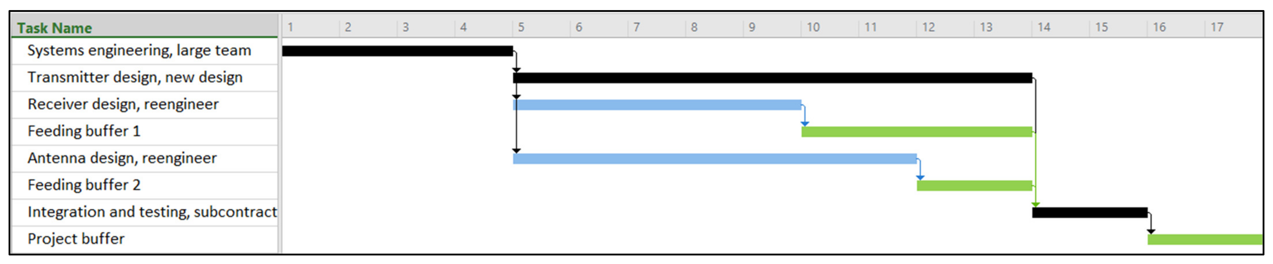
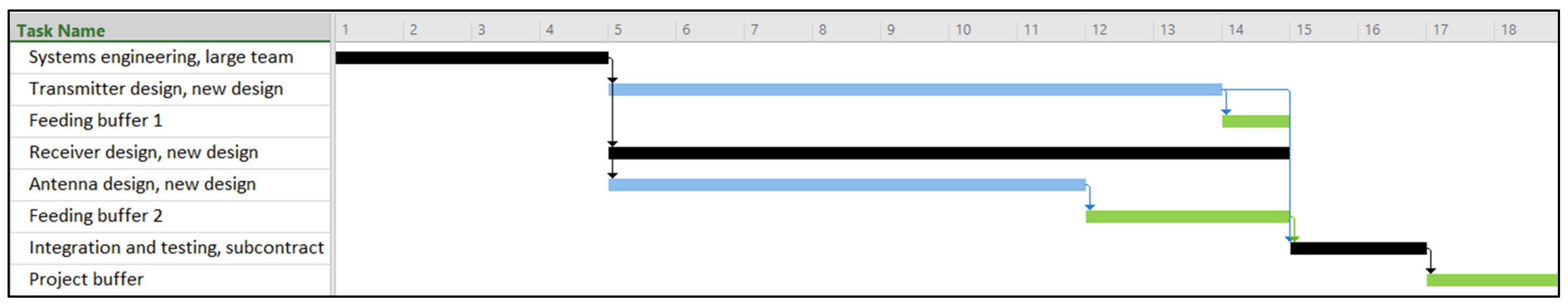
Once a baseline schedule is established, the PBs and FBs are inserted using a buffer-sizing technique such as the methods discussed in Section 2.2. The aim is to create a stable schedule that can be evaluated using robustness measures described in relevant literature, such as the standard deviation of project length, stability cost, and timely project completion probability [44].

The on-time probability not only serves as an indicator of schedule robustness but also plays a role in buffer calculation. Hoel and Taylor [26] proposed the use of Monte Carlo simulation to determine the cumulative distribution function (CDF) for project completion time, thereby determining the size of the PB. For example, if we aim for a 95% probability of completing the project on schedule, the PB would be the difference between the project duration at the 95th percentile and the duration of the baseline schedule.

Let us go one step further. If we directly search for the shortest time-buffered schedule that meets the desired on-time probability, we can identify a schedule with the same probability but a shorter duration. This leads us to the chance-constrained CCBM problem, where we consider multimode projects. In this problem formulation, we not only search for the schedule but also determine the activity modes that result in the shortest project duration while meeting the desired on-time probability. This duration encompasses the baseline schedule, nominal (deterministic) activity durations, and the PB. In this paper, we define project delivery as this time-buffered project duration, which represents the deadline we can meet (i.e., deliver the project) with the desired on-time probability.

To model our chance-constrained CCBM problem, we adopt a MILP approach using the flow-based formulation described in [84], extending it to accommodate multimode projects. We handle the chance constraints using SA as in the LPM model but require additional parameters and decision variables that were not present there.

There are K distinct renewable resources available, each having a total availability of ${ℛ}^k$ units. When activity j is executed in mode m, it requires $r_{jm}^k$ units of resource k. For a given scenario s, the earliest start time for activity j is denoted as $E{S}_{js}$, while $L{S}_{js}$ represents the latest start time.

The project delivery is represented by decision variable $D_p$. Project milestones 0 and $J+1$ have a singular mode, zero duration, and no resource requirements. Binary decision variable $z_{ij}$ is employed to indicate if activity j commences after the completion of activity i, taking a value of 1 in such cases. The flow variable ${\varphi }_{ij}^k$ models the amount of resource k transferred from activity i to activity j.

Our chance-constrained CCBM model incorporates constraints (3), (8), (12), and (16) from the LPM model. Moving forward, we will present the model, followed by an explanation of the objective function and the remaining constraints.

$$\mathrm{Min} D_p,$$

(18)

subject to:

$$t_{J+1,s}-\theta \left(1-{\tau }_s\right)\le D_p,\hspace{1em}\forall s=1,\dots ,S,$$

(19)

$$z_{ij}+z_{ji}\le 1,\hspace{1em}\forall i=0,\dots ,J,\hspace{1em}\forall j=1,\dots ,J+1,\hspace{1em}\forall i<j,$$

(20)

$$z_{ij}+z_{jh}-z_{ih}\le 1,\hspace{1em}\forall i,j,h=0,\dots ,J+1,\hspace{1em}\forall i\ne j\ne h,$$

(21)

$$z_{ij}=1,\hspace{1em}\forall i\in Ƥ\left(j\right),\hspace{1em}\forall j=1,\dots ,J+1,$$

(22)

$$t_{js}-t_{is}-M{z}_{ij}\ge {\displaystyle \sum _{m=1}^{M_i}{\delta }_{im}}{d}_{ims}-M,\hspace{1em}\forall i,j=0,\dots ,J+1,\hspace{1em}\forall i\ne j,\hspace{1em}\forall s=1,\dots S,$$

(23)

$$E{S}_{js}\le t_{js}\le L{S}_{js},\hspace{1em}\forall j=0,\dots ,J+1,\hspace{1em}\forall s=1,\dots ,S,$$

(24)

$$\begin{array}{l}{\varphi }_{ij}^k-\min \left({\tilde{r}}_{im}^k,{\tilde{r}}_{j{m}^{\prime }}^k\right)z_{ij}-\left(1-{\delta }_{im}\right)\left({\tilde{r}}_{ij}^{\max ,k}-\min \left({\tilde{r}}_{im}^k,{\tilde{r}}_{j{m}^{\prime }}^k\right)\right)\\ -\left(1-{\delta }_{j{m}^{\prime }}\right)\left({\tilde{r}}_{ij}^{\max ,k}-\min \left({\tilde{r}}_{im}^k,{\tilde{r}}_{j{m}^{\prime }}^k\right)\right)\le 0,\hspace{1em}\mathrm{where} r_{ij}^{\max ,k}=\max \left(\underset{m=1,\dots ,M_i}{\max }{\tilde{r}}_{im}^k,\underset{m^{\prime }=1,\dots ,M_j}{\max }{\tilde{r}}_{j{m}^{\prime }}^k\right),\\ \forall i=0,\dots ,J,\hspace{1em}\forall j=1,\dots ,J+1,\hspace{1em}\forall i\ne j,\hspace{1em}\forall k=1,\dots ,K,\hspace{1em}\forall m=1,\dots ,M_i,\hspace{1em}\forall m^{\prime }=1,\dots ,M_j,\\ \mathrm{where} {\tilde{r}}_{jm}^k=\{\begin{array}{l}{r}_{jm}^k \mathrm{if} 0<j<n+1\hfill \\ R^k \mathrm{if} j=0 \mathrm{or} j=n+1,\hfill \end{array}\end{array}$$

(25)

$${\displaystyle \sum _{j\in \left\{1,\dots ,J+1\right\}\backslash \left\{i\right\}}{\varphi }_{ij}^k={\displaystyle \sum _{m=1}^{M_i}{\tilde{r}}_{im}^k{\delta }_{im}},\hspace{1em}\forall i=0,\dots ,J,\hspace{1em}\forall }k=1,\dots ,K,$$

(26)

$${\displaystyle \sum _{i\in \left\{0,\dots ,J\right\}\backslash \left\{j\right\}}{\varphi }_{ij}^k={\displaystyle \sum _{m=1}^{M_j}{\tilde{r}}_{jm}^k{\delta }_{jm}},\hspace{1em}\forall j=1,\dots ,J+1},\hspace{1em}\forall k=1,\dots ,K,$$

(27)

$$\begin{array}{l}0\le {\varphi }_{ij}^k\le \min \left(\underset{m=1,\dots ,M_i}{\max }{\tilde{r}}_{im}^k,\underset{m=1,\dots ,M_j}{\max }{\tilde{r}}_{jm}^k\right),\hspace{1em}\forall i=0,\dots ,J,\hspace{1em}\forall j=1,\dots ,J+1,\hspace{1em}\forall i\ne j,\\ \forall k=1,\dots ,K.\end{array}$$

(28)

The objective function (18) is designed to minimize the project’s delivery time. Constraints (19) indicate whether a scenario is completed within the desired timeframe. Constraints (20) and (21), derived from previous works [84,85], prevent cycles of 2 or 3 or more activities. Constraints (22) enforce the precedence relationships between activities. Constraints (23) establish the relationship between continuous activity start time variables and binary sequencing variables. Constraints (24) define upper and lower bounds for activity start times. Constraints (25), drawing from [85], establish a connection between the continuous resource flow variables, binary sequencing variables, and mode variables.

Outflow constraints (26) guarantee that all activities, except for milestone $J+1,$ transfer their resources (when finished with them) to other activities. Inflow constraints (27) ensure that all activities, except for milestone 0, receive their resources from other activities. Constraints (28) set bounds on the flow variables based on the maximum resource consumption modes.

It is important to note that the general constraints (25) and (28) can be reformulated as MIP constraints using linear and special-ordered set constraints, along with auxiliary variables [86]. Commercial solvers such as Gurobi automatically handle the equivalent formulation (in [85], these constraints are also handled by the solver).

Once the MILP is solved, constructing a schedule follows a straightforward approach. The project is represented as an activity-on-node (AON) network, with arcs connecting activities j to their immediate predecessors $Ƥ\left(j\right)$. If resources flow from activity i to j, j cannot start before i finishes, making i an immediate predecessor of j. Hence, we add arcs between activities wherever ${\varphi }_{ij}^k>0$. This construction, referred to as a resource flow network [87], can be achieved by simply adding i to $Ƥ\left(j\right)$. Finally, we schedule all activities using the “early start” approach, where each activity commences when its immediate predecessor concludes.

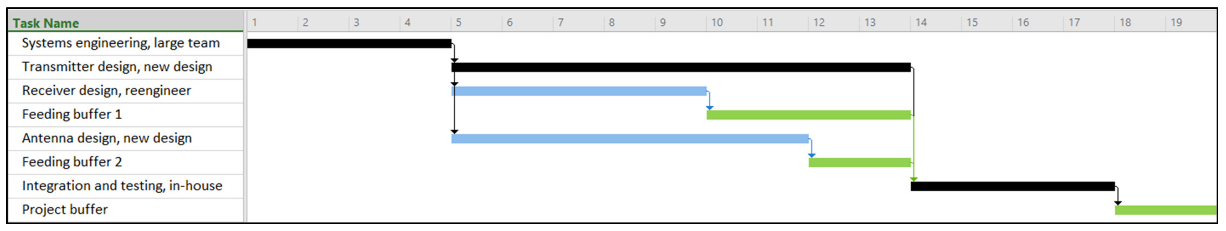
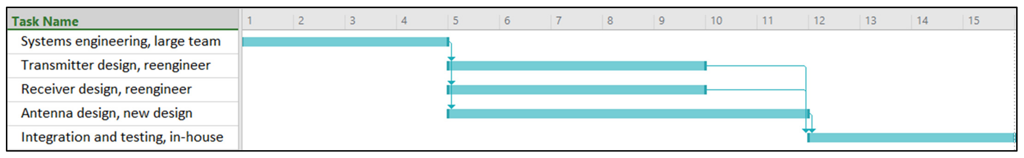
For the baseline schedule, the activity duration used is typically the most likely duration based on a three-point estimate. After the completion of the last activity, the PB is inserted, calculated as the difference between the project delivery time and the baseline duration. An example illustrating this approach can be found in Section 6.

To insert FBs, we adopt the method proposed by [26] and applied in subsequent works, e.g., [88,89] (the latter employing the method as an upper bound for the buffers). In this approach, activities are scheduled using an “early start” strategy, and the FB is determined based on the free float of the activity that merges into the critical chain, ensuring that no new resource conflicts arise from the insertion of FBs. Thus, since we initiate all activities as early as possible, we can disregard the size of FBs in our problem.

Our CCBM model is extremely significant for project management applications, especially for addressing uncertainties and risks in project scheduling. The objective function and chance constraints allow the project manager to produce time-buffered project plans that minimize the project delivery date while staying within the stakeholders’ risk threshold. In the Introduction, we discussed the importance of this topic, and in Section 2.2, we discussed the limitations of existing scheduling methods. In Section 8, we demonstrate the effectiveness of the proposed CCBM model in producing shorter project durations compared with established benchmarks.

4.3. TVNPV

In line with Section 4.2, we utilize the flow-based formulation introduced by [84] and extend it to encompass multimode projects, NPV, value functions, and chance constraints. The primary objective of the TVNPV model is to maximize the robust project NPV and the project value. To address the chance constraints, we employ SA. We now describe additional parameters and decision variables that are not present in the LPM and CCBM models.

Within the problem context, we have K distinct renewable resources, each associated with a unit cost $c_k$ per period. Additionally, activity j executed in mode m incurs a fixed cash inflow or outflow $c_{jm},$ consisting of fixed costs and payments received. For convenience, we assume that payments are received or made at the end of each activity. To avoid gaps between activities and prevent indefinitely postponing activities with negative cash flows, two main approaches exist in the literature: (1) utilizing a deadline [57] and (2) assuming a sufficiently large payout at the end of the project to offset the gains from postponing activities impacting project completion [66]. In this paper, we adopt the latter approach.

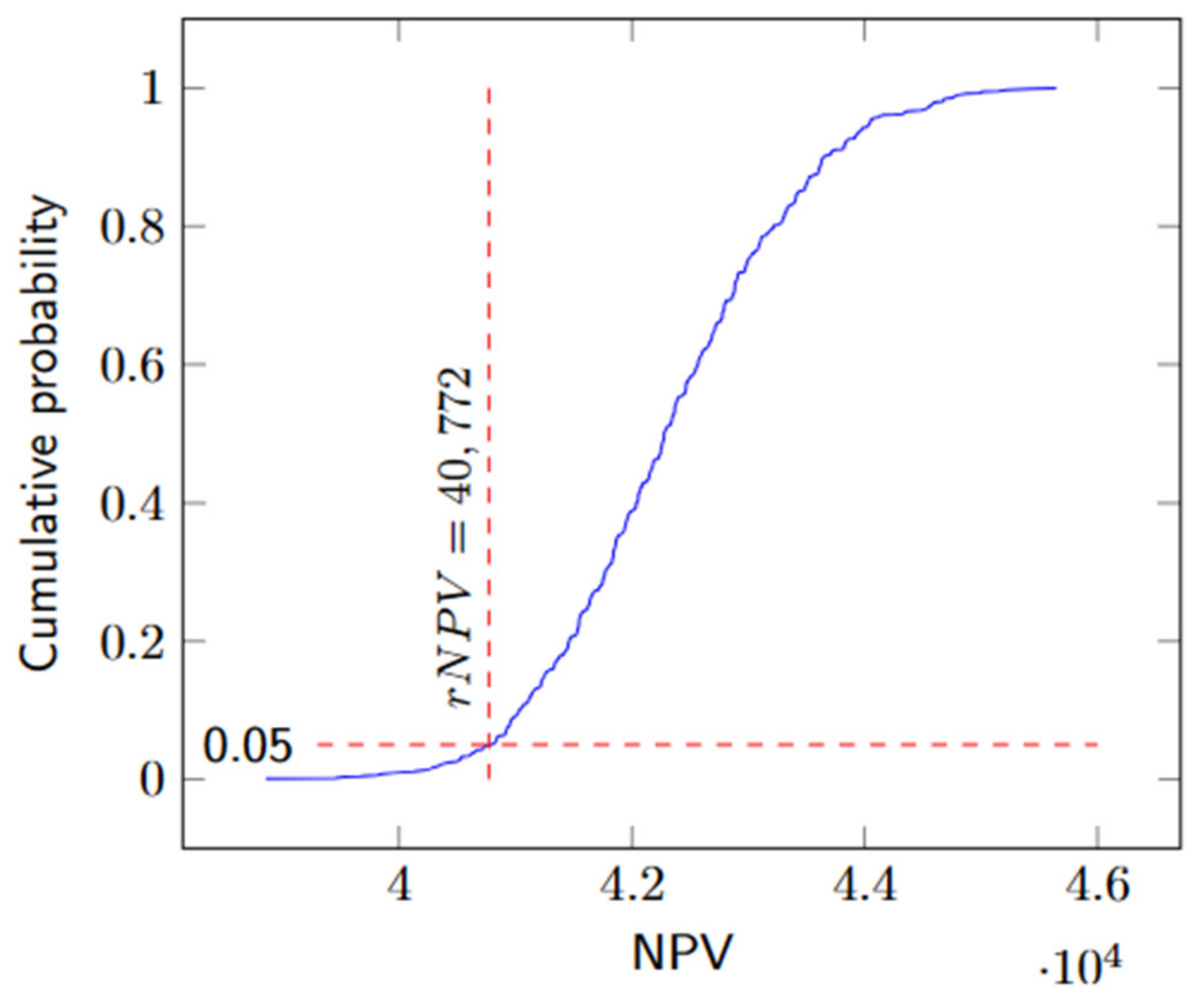
When aiming to minimize project duration, a common measure of robustness is the timely project completion probability [44]. In our problem, we adapt this concept and introduce the decision variable rNPV to represent the robust NPV. It signifies the project NPV achieved with a probability of at least γ. Thus, instead of evaluating the robustness of a given schedule, we search directly for a schedule with the desired level of robustness.

Several parameters are defined within the model. $NP{V}^{UP}$ serves as an upper bound for rNPV. $\stackrel{⌢}{r}$ denotes the discount rate, while $E{F}_{js}$ and $L{F}_{js}$ represent the earliest and latest finish times for activity j in scenario s, respectively. Additionally, $T_{\max }$ acts as an upper bound for the project’s duration.

To represent the finish time of activity j in scenario s, we introduce the decision variable $f_{js}\in \{E{F}_{js},\dots ,L{F}_{js}\}$. Binary variable ${\tilde{\tau }}_s$ takes the value 1 if the scenario NPV is greater than rNPV. Moreover, decision variable ${\beta }_{js}$ represents the discount factor for activity j in scenario s, and ${\beta }^{UP}$ serves as an upper bound for the discount factor.

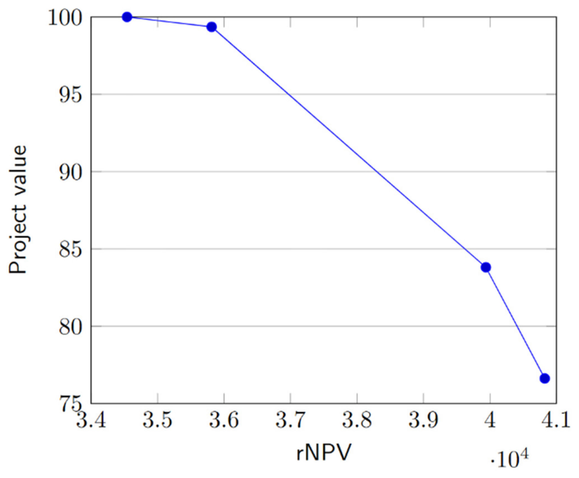
Objective function weights $w_1$ and $w_2$ are included to determine the tradeoff between rNPV and the project value. By solving the MIP for different values of $w_1$ and $w_2,$ we can identify the efficient frontier that balances these objectives.

To linearize two sets of constraints, we introduce additional variables. Binary variables $t_{js}^p$ are assigned a value of 0 for all $p<f_{js}$ and 1 for all $p\ge f_{js}, p=0,\dots ,T_{\max }$. Variables $y_{jms}$ replace the products ${\beta }_{js}{\delta }_{jm}$. The model incorporates constraints (2), (3), (8), (20)–(22), and (25)–(28) from the LPM and CCBM models.

We now present the model, providing an explanation of the objective function, followed by an overview of the remaining constraints. Subsequently, we will discuss the linearization of the nonlinear constraints.

$$\mathrm{Max}\left(w_{1}rNPV+w_2{V}^{″}\left(F_1\left({V^{\prime }}_{11},\dots ,{V^{\prime }}_{J1}\right),\dots ,F_V\left(V_{\prime }^{1V},\dots ,V_{\prime }^{JV}\right)\right)\right),$$

(29)

subject to:

$${\displaystyle \sum _{j=0}^{J+1}{\displaystyle \sum _{m=1}^{M_j}\left(c_{jm}+{\displaystyle \sum _{k=1}^K{c}_k{r}_{jkm}{d}_{jms}}\right)}}{\beta }_{js}{\delta }_{jm}+NP{V}^{UP}\left(1-{\tilde{\tau }}_s\right)\ge rNPV,\hspace{1em}\forall s=1,\dots ,S,$$

(30)

$${\beta }_{js}={\left(1+\stackrel{⌢}{r}\right)}^{-f_{js}},\hspace{1em}\forall j=0,\dots ,J+1, \forall s=1,\dots ,S,$$

(31)

$${\displaystyle \sum _{s=1}^S{\tilde{\tau }}_s\ge \gamma S,}$$

(32)

$$f_{js}-{\displaystyle \sum _{m=1}^{M_j}{\delta }_{jm}}{d}_{jms}-M{z}_{ij}\ge f_{is}-M,\hspace{1em}\forall i,j=0,\dots ,J+1,\hspace{1em}\forall i\ne j,\hspace{1em}\forall s=1,\dots S,$$

(33)

$$E{F}_{js}\le f_{js}\le L{F}_{js},\hspace{1em}\forall j=0,\dots ,J+1,\hspace{1em}\forall s=1,\dots ,S,$$

(34)

The primary objective of the model, captured in the objective function (29), is to maximize a weighted sum of the project’s rNPV and its overall value. This approach, known as the weighted-sum method, is widely employed in multi-objective optimization [90] and has been utilized in various project scheduling studies, e.g., [72,91,92].

To ensure the robustness of the project’s NPV, constraints (30) are introduced, which evaluate whether a scenario’s NPV surpasses the project’s rNPV. Inspired by [93], we adopt a discrete discount factor in constraints (31). Constraint (32) is employed to monitor the fraction of scenarios that yield the desired rNPV, enforcing this fraction to remain above a predetermined threshold.

The interdependence between the continuous activity finish time variables and the binary sequencing variables is established through constraints (33). Additionally, constraints (34) provide necessary bounds for the activity’s finish times.

Constraints (30) pose a challenge due to the nonlinearity arising from the product of the discount factor and the indicator variable, ${\beta }_{js}{\delta }_{jm}$. To address this nonlinearity, we replace constraints (30) with constraints (35) that involve auxiliary variables, denoted as $y_{jms}$. To ensure the equivalence of $y_{jms}$ and ${\beta }_{js}{\delta }_{jm}$, constraints (36)–(39) are introduced to maintain the relationship between these variables within the model.

$${\displaystyle \sum _{j=0}^{J+1}{\displaystyle \sum _{m=1}^{M_j}{y}_{jms}\left(c_{jm}+{\displaystyle \sum _{k=1}^K{c}_k{r}_{jkm}{d}_{jms}}\right)}}+NP{V}^{UP}\left(1-{\tau }_s\right)\ge rNPV,\hspace{1em}\forall s=1,\dots ,S,$$

(35)

$$y_{jms}\le {\beta }^{UP}{\delta }_{jm},\hspace{1em}\forall j=0,\dots ,J+1,\hspace{1em}\forall m=1,\dots ,M_j,\hspace{1em}\forall s=1,\dots ,S,$$

(36)

$$y_{jms}\le {\beta }_{js},\hspace{1em}\forall j=0,\dots ,J+1,\hspace{1em}\forall m=1,\dots ,M_j,\hspace{1em}\forall s=1,\dots ,S,$$

(37)

$$y_{jms}\ge {\beta }_{js}-\left(1-{\delta }_{jm}\right){\beta }^{UP},\hspace{1em}\forall j=0,\dots ,J+1,\hspace{1em}\forall m=1,\dots ,M_j,\hspace{1em}\forall s=1,\dots ,S,$$

(38)

$$y_{jms}\ge 0,\hspace{1em}\forall j=0,\dots ,J+1,\hspace{1em}\forall m=1,\dots ,M_j,\hspace{1em}\forall s=1,\dots ,S.$$

(39)

To replace the exponential discount factor from constraints (31), we introduce linear constraints (40) into the model. Additionally, we incorporate the following constraints into the model:

• Constraints (41) establish a connection between the binary variables $t_{js}^p$ and $f_{js}$.
• Constraints (42) ensure that an activity can only have a single finish time.
• Constraints (43) impose bounds on $t_{js}^p,$ as the predecessor will always have a value of 1 before its successor.
• Constraints (44) and (45) fix the value of $t_{js}^p$ for finish times occurring before the early finish and after the late finish, respectively.
• Finally, constraints (46) determine the fixed value for the initial milestone.

$${\beta }_{js}={\displaystyle \sum _{p=1}^{T_{\max }}{\left(1+\stackrel{⌢}{r}\right)}^{-p}\left(t_{js}^p-t_{js}^{p-1}\right)},\hspace{1em}\forall j=0,\dots ,J+1,\hspace{1em}\forall s=1,\dots ,S,$$

(40)

$${\displaystyle \sum _{p=1}^{T_{\max }}p\left(t_{js}^p-t_{js}^{p-1}\right)}=f_{js},\forall j=0,\dots ,J+1,\forall s=1,\dots ,S,$$

(41)

$${\displaystyle \sum _{p=1}^{T_{\max }}\left(t_{js}^p-t_{js}^{p-1}\right)}=1,\hspace{1em}\forall j=1,\dots ,J+1,\hspace{1em}\forall s=1,\dots ,S,$$

(42)

$$t_{is}^p\ge t_{js}^p, \forall i\in \left(j\right),\hspace{1em}\forall j=1,\dots ,J+1,\hspace{1em}\forall p=0,\dots ,T_{\max },\hspace{1em}\forall s=1,\dots ,S,$$

(43)

$$t_{js}^p=0,\hspace{1em}\forall j=1,\dots ,J+1,\hspace{1em}\forall p=0,\dots ,E{F}_j-1,\hspace{1em}\forall s=1,\dots ,S,$$

(44)

$$t_{js}^p=1,\hspace{1em}\forall j=1,\dots ,J+1,\hspace{1em}\forall p=L{F}_j+1,\dots ,T_{\max },\hspace{1em}\forall s=1,\dots ,S,$$

(45)

$$t_{0,s}^p=1,\hspace{1em}\forall p=0,\dots ,T_{\max },\hspace{1em}\forall s=1,\dots ,S.$$

(46)

We can use a commercial solver to solve the MIP if the value function of the project is linear because the constraints are linearized, as explained before. This method is our benchmark for the computational experiments that we present in Section 7.

Our TVNPV model is very useful and suitable for project management in various aspects. Firstly, the objective function and the chance constraints aim to maximize both project value and NPV. This is a new and useful tool for decision-making because it allows the generation of project plans on the efficient frontier with different optimal combinations of value and NPV. Secondly, the uncertainties in activity durations and the chance constraints enable the calculation of a robust NPV according to the stakeholders’ tolerance for risk. Additionally, the model employs a multimode approach that evaluates the impact of mode selection on project cost, duration, resources, and value.

5. The RL Solution

RL has demonstrated remarkable achievements in various domains, ranging from mastering backgammon at a level comparable to the world’s best players [94] to successfully landing unmanned aerial vehicles (UAVs) [95], defeating top-ranked contestants in Jeopardy! [96], and achieving human-level performance in Atari games [97]. These accomplishments highlight the effectiveness of RL in dealing with uncertain environments. Inspired by this success, we apply RL to the formulations described in Section 4. While RL-based heuristics have been employed in project scheduling [98,99], to the best of our knowledge, no previous work has addressed multimode problems with chance constraints using RL.

The RL framework begins by placing an agent in a state denoted as S. The agent takes an action denoted as A and transitions to state ${\mathcal{S}}^{\prime },$ receiving a reward denoted as ${ℛ}^{\prime }$. Subsequently, the agent performs action ${\mathcal{A}}^{\prime },$ moves to state ${\mathcal{S}}^{″},$ and receives reward ${ℛ}^{″},$ and the pattern continues. Hence, the agent’s life trajectory can be represented as $\mathcal{S},\mathcal{A},{ℛ}^{\prime },{\mathcal{S}}^{\prime },{\mathcal{A}}^{\prime },{ℛ}^{″},{\mathcal{S}}^{″},{\mathcal{A}}^{″},{ℛ}^{‴},{\mathcal{S}}^{‴},{\mathcal{A}}^{‴},$ and so on. To guide the agent’s behavior in each state, a policy denoted as $\pi \left(\mathcal{S},\mathcal{A}\right)$ is followed, instructing the agent which action to take. The objective of the RL problem is to learn a policy that maximizes the agent’s cumulative reward. Additionally, we introduce an action-value function denoted as $q\left(\mathcal{S},\mathcal{A}\right),$ which estimates the reward for taking action A in state S and subsequently following policy $\pi \left(\mathcal{S},\mathcal{A}\right)$.

By applying the RL model to the formulations outlined in Section 4, we define a state as a project activity denoted by j. The agent takes action by selecting a mode ${\widehat{m}}_j$ and additionally, in CCBM and TVNPV, a start time ${\widehat{t}}_j$ for activity j, and then proceeds to the next activity. After determining modes and start times for all activities $j=1,\dots ,J,$ the agent can calculate its reward $ℛ\left(j,m,t\right)$. As the agent receives rewards, it learns the action-value function $q\left(j,m,t\right)$ and the corresponding policy $\pi \left(j,m,t\right)$ to be followed.

In this study, we utilize Monte Carlo control (MCC), an RL method based on [100]. MCC leverages Monte Carlo simulation to estimate CDFs for the activity durations, which are used in reward calculations. The algorithms for each of the three problems consist of a main procedure in which multiple functions are called. This section presents the main procedures along with a high-level explanation. The pseudocode and detailed explanations for each function can be found in Appendix A.

The LPM main procedure is shown in Algorithm 1. The iterative process comprises three key steps:

• Policy calculation: The policy is a table of the probabilities of the agent taking each action. In our case, this means selecting a mode for each activity. We employ a technique called ε-greedy policies, where we examine the action-value table and assign a probability ε of picking a random mode for an activity. Otherwise, we pick the mode with the highest action-value.
• Reward computation: We use the policy to select the modes and then compute the reward for this action. In LPM, we model the reward as the project value, calculated by the project-specific value function. For an example of a value function, see Section 6.
• Action-value update: The reward obtained by this choice of modes is used to update the action-value table. To calculate the new action-values, we either average all the rewards obtained for this specific mode choice (RL₁) or use a constant-step formula (RL₂). For more details on these action-value update variants, see Appendix A.

Algorithm 1: Main MCC procedure for LPM.

initialize_action_values from Algorithm A1

while not stopping criterion:

calculate_policy from Algorithm A2

calculate_reward from Algorithm A3

update_action_values_RL1 from Algorithm A4   or update_action_values_RL2 from Algorithm A5

If the stopping criterion is not met, the policy is recalculated based on the updated action-values, initiating a new iteration of the cycle.

The main procedure for the CCBM model is shown in Algorithm 2. Focusing on the features that differ from the previous LPM–RL algorithm, in CCBM, an action consists of selecting a start time for an activity in addition to the mode. Regarding the reward, we construct an early-start resource-feasible baseline schedule and model the reward as the reciprocal of the delivery date, defined in Section 4.2.

Algorithm 2: Main procedure for MCC for CCBM and TVNPV.

initialize_action_values from Algorithm A6

while not stopping criterion:

calculate_policy from Algorithm A7

choose_mode_start from Algorithm A8

calculate_reward from Algorithms A9 and A10

update_action_values_RL1 from Algorithm A4   or update_action_values_RL2 from Algorithm A5

Finally, regarding the TVNPV RL algorithm, the difference between it and the previous CCBM is the reward calculation. The reward is the objective function value, which is the weighted sum between rNPV and project value. Instead of an early-start schedule, the project activities are scheduled according to the selected start-time action. This way, we account for cash inflows and outflows, since in the latter case, it is advantageous to postpone an activity instead of starting it early.

6. Example

To provide a concrete illustration of our problem and the RL solution approach, let us consider as an example the development of a radar system, drawn from a real-world project. In Figure 2, we present the project’s AON network, while

Table 1. Summary of data for radar development.

Activity	Mode	Duration			FC	Resources			Value Parameters			Income
		O	ML	P		E	T		R	Q	Re
Systems engineering	Small team	5	7	10	2000	1	0			0.8
	Large team	3	4	4	4000	3	1			0.99
Transmitter design	Reengineer	3	5	8	5000	2	1		50	0.99	0.9	52,500
	New design	7	9	11	10,000	4	2		100	0.95	0.8
Receiver design	Reengineer	3	5	9	2000	2	1		30	0.95	0.9
	New design	8	10	11	15,000	3	1		200	0.8	0.99
Antenna design	Reengineer	3	7	9	3000	3	2		10	0.8	0.9
	New design	6	7	9	7000	5	2		30	0.99	0.9
Integration and testing	In-house	3	4	4	4000	3	3			0.99	0.9	20,000
	Subcontract	2	2	5	6000	1	0			0.9	0.99

provides a list of the project’s five activities, each with two available modes. The table includes the optimistic, most likely, and pessimistic durations (O, ML, and P) of the activities, their respective fixed costs (FC), the required resources per period for each mode (engineers, E, and technicians, T), the value parameters, and the income received upon activity completion.

It is worth noting that three of the five activities exhibit negative cash flows, i.e., fixed and resource costs, while the remaining two activities yield positive cash flows due to the generated income. This example effectively illustrates how value is defined and measured in practice. The needs and expectations of project stakeholders are translated into value attributes such as range, quality, and reliability (R, Q, and Re, respectively, as shown in Table 1). These attributes are determined by the value parameters associated with each activity mode. Additionally, it is important to consider the resource unit costs per period, which amount to USD 100 for engineers and USD 50 for technicians.

In the context of the radar system, we employ the radar equation [101] for computing the radar range [21]. The quality and reliability of the radar system are also considered, as they depend on technical parameters such as transmitter power and antenna gain. These parameters, in turn, are contingent upon the technological alternatives available for each mode. The selection of a mode for the project plan not only determines its value but also has a significant impact on cost and NPV, effectively integrating both components of project value.

The equation for calculating radar range $F_1={\left(\left[TP\right]\left[RS\right]\left[AG\right]\right)}^{0.25}$ involves the variables $\left[TP\right]$ (transmitter power), $\left[RS\right]$ (receiver sensitivity), and $\left[AG\right]$ (antenna gain). These parameters are extracted from the corresponding activities in Table 1—namely, transmitter design, receiver design, and antenna design. Similarly, the equation for radar quality $F_2=100\left[SEQ\right]\left[QT\right]\left[QR\right]\left[QA\right]\left[QI\right]$ incorporates the impact of various factors denoted by $\left[SEQ\right],$ $\left[QT\right],$ $\left[QR\right],$ $\left[QA\right]$, and $\left[QI\right],$ which represent systems engineering, transmitter, receiver, antenna, and integration effects on quality, respectively. Likewise, the equation for radar reliability $F_3=100\left[AR\right]\left[IR\right]\left[TR\right]\left[RR\right]$ considers the contributions of antenna design, integration effort, transmitter reliability, and receiver reliability, represented by $\left[AR\right],$ $\left[IR\right],$ $\left[TR\right],$ and $\left[RR\right],$ respectively. Finally, the project value is determined by computing a weighted sum of the three value attributes, a widely used technique in multi-attribute utility theory [102] expressed as $V^{″}=\raisebox{1ex}{$7$}\!\left/ \!\raisebox{-1ex}{$21$}\right.F_1+\raisebox{1ex}{$8$}\!\left/ \!\raisebox{-1ex}{$21$}\right.F_2+\raisebox{1ex}{$6$}\!\left/ \!\raisebox{-1ex}{$21$}\right.F_3$. We now illustrate this example within the context of the three challenges presented in this paper: LPM, CCBM, and TVNPV.

6.1. LPM

Here we address the optimization of activity modes and start times to maximize the project value while ensuring a 95% probability of meeting both the schedule and budget requirements. The project is characterized by a due date of 17 time periods and a budget of USD 39,800. To achieve our objective, we employed the RL₁ algorithm and terminated the iterations when no further improvement in the maximum project value was observed over the last 100 iterations.

To facilitate analysis and comparison, we normalized the project values on a scale of 0 to 100, following the approach outlined by [5]. The solution obtained from the algorithm is presented in the form of a Gantt chart (Figure 3). It is important to note that the activity durations shown on the Gantt chart correspond to the most likely (nominal) durations (Table 1). For example, for the activity “systems engineering”, mode “large team”, the most likely duration is four time periods.

The project plan resulting from this optimization approach achieved a project value of 58.365, which, after normalization, corresponds to a value of 100. The nominal cost associated with this plan is USD 31,900. Furthermore, the probability of completing the project on time is 100%, while the probability of staying within the budget stands at 99%.

As outlined in Section 5, our search process is guided by learning and updating the action-value table, which subsequently leads to the recalculation of the ε-greedy policy. To illustrate this approach, we provide an overview of the action-value evolution in

Table 2. LPM: evolution of action-values for the radar project.

Optimistic initial values			Iteration 10			Iteration 20			Iteration 30
Act	Mode1	Mode2	Act	Mode1	Mode2	Act	Mode1	Mode2	Act	Mode1	Mode2
1	999	999	1	0	100	1	0	82.43	1	0	85.14
2	999	999	2	88.89	0	2	82.43	0	2	85.14	0
3	999	999	3	88.89	0	3	87.28	0	3	91.69	0
4	999	999	4	0	88.89	4	41.91	77.78	4	41.91	82.14
5	999	999	5	88.89	0	5	78.1	0	5	80.15	75.0
Iteration 40			Iteration 50			Iteration 100			Iteration 119
Act	Mode1	Mode2	Act	Mode1	Mode2	Act	Mode1	Mode2	Act	Mode1	Mode2
1	0	86.42	1	0	84.42	1	0	86.63	1	0	87.7
2	88.75	0	2	86.25	0	2	88.43	11.86	2	89.21	11.86
3	91.22	0	3	88.17	0	3	88.5	0	3	90.07	0
4	41.91	84.21	4	55.87	80.85	4	71.69	82.98	4	74.72	84.68
5	82.88	75.0	5	79.73	75.0	5	82.94	75.0	5	84.66	75.0

, showcasing the progression from the initial optimistic values to the latest iteration.

One significant advantage of our solution is its ability to support decision-making by generating an efficient frontier of project plans that incorporate the inherent uncertainty of project durations. This empowers tradeoff analysis, enabling the selection of the optimal plan based on a careful balance between risk and value considerations.

To exemplify the practical application of our approach, let us consider a scenario in our radar project example where the decision-makers aim to reduce the budget by USD 13,300, adjust the due date to 18 time periods, and ascertain the achievable value for the stakeholders. The efficient frontier for this particular case is depicted in Figure 4.

When examining the scenario where the on-time probability stands at 80% and the on-budget probability at 70%, it becomes apparent that the project is deemed infeasible. If, however, the decision-makers are willing to accept a lower on-budget probability of 60%, it becomes possible to achieve the maximum value, approximately 83. This observation highlights the substantial impact of a constrained budget on the project’s capacity to provide value to stakeholders. It underscores the significance of incorporating stochastic activity durations to accurately portray the value that the project can deliver to its stakeholders.

6.2. CCBM

In this and Section 6.3, we consider a scenario where there are 11 engineers and four technicians available to work on the project. Our goal is to find the shortest project duration that satisfies a given probability β of completing the project on time. Gantt charts illustrating the project activities, selected modes, FBs, and PBs are presented in Figure 5, Figure 6 and Figure 7. These charts showcase the solutions achieved for different desired probabilities, namely, 90%, 95%, and 100%. The baseline schedule activity durations correspond to the most likely durations from Table 1.

As anticipated, the lower the level of risk we are willing to tolerate, indicated by a higher on-time probability, the longer the duration of the buffered project grows. It is intriguing to observe the progressive improvement in solutions achieved by our RL agent. In our RL model, we defined the reward as the reciprocal of the project duration. Figure 8 displays the learning curves for both variants of action-value updating, RL₁ and RL₂, focusing on a 95% on-time probability. At the initial stages of the curves, the influence of optimistic initial values (described in Section 5) is evident: despite discovering the minimum delivery duration early on, the agent continued to explore randomly, under the impression that it might obtain a better reward by pursuing alternative actions, given the artificially inflated values in the action-value list. Eventually, the delivery duration stabilized at 18 time periods. As we employed ε-greedy policies (outlined in Section 5), the agent occasionally explored, resulting in intermittent deviations from the minimum delivery duration.

6.3. TVNPV

We aim to address the problem by considering different weights, w₁ and w₂, and obtaining the efficient frontier for a 95% probability of rNPV. The resulting frontier, consisting of four non-dominated points, is depicted in Figure 9. Decision makers can perform a tradeoff analysis to select the solution that best aligns with stakeholders’ needs and requirements.

As discussed in Appendix A.3, rNPV is determined iteratively by simulating the NPV CDF. In Figure 10, the CDF plot illustrates the rNPV for the point (76.62, 40,772) in Figure 9. With the decision makers’ chosen solution, a baseline schedule can easily be constructed using the process outlined in Algorithm A10 and explained in Appendix A.3. The resulting Gantt chart is presented in Figure 11. Figure 12 showcases the learning curves for both RL₁ and RL₂, demonstrating how our action-value updating variants evolve over time.

7. Experimental Setting

The experiments were conducted to validate the effectiveness of our RL procedure in solving the formulations outlined in Section 4. We utilized the PSPLIB dataset [103], which consists of 535 project instances with 10 activity projects and three activity modes per project. This dataset is widely recognized as the standard in the literature on multimode project management [104].

To generate scenarios and simulate runs, we employed three-point estimates for activity mode durations. Specifically, we defined the dataset’s duration as the most likely duration, with the optimistic duration set at half this value and the pessimistic duration set at 2.25 times the most likely duration. These multipliers align with the characteristic right-skewed distribution of activity durations in project management [47]. Realized durations were randomly drawn from a triangular distribution, a common approach in project simulation [105], and rounded to the nearest integer.

Our RL algorithms were executed using two different methods for updating the action values, RL₁ and RL₂, as described in Section 5. We maintained the same probability of a random action (ε = 0.1) and constant step-size parameter (α = 0.1) as specified in [100]. To solve the MILP problems in the benchmarks, we employed the Python interface for Gurobi solver version 9.0. All algorithms were implemented in Python.

The experiments were conducted on a computer equipped with an Intel(R) Core(TM) i7-7700 CPU 3.60 GHz and 8 GB RAM. For data analysis, we performed pairwise comparisons of the objective function values generated by each method. We utilized JMP statistical software to calculate the p-values for Wilcoxon signed rank (WSR) tests with a significance level of 0.05.

Below, we provide specific details of the experimental design for each of the three problems discussed in this paper.

7.1. LPM

We compared the project values obtained from our variants to those of two benchmarks: a genetic algorithm (GA) and a solution for our MILP problem (Section 4.1). GAs are widely used for solving project scheduling problems [106], which motivated our selection of a GA as a benchmark. We used the specialized GA proposed by [5] with minor modifications, as it is specifically designed for value functions and closely aligned with our problem. The GA parameters included a population size of 500, percentiles for elite and worst solutions, and a mutation probability of 0.1.

Since the GA fitness function in [5] was designed for deterministic problems only, we developed a new fitness function suitable for our stochastic settings (details in Appendix A). To ensure a fair comparison, we terminated RL₁ and RL₂ at the point when the GA converged according to its published stopping criterion, i.e., when the best value remained unchanged for two consecutive generations. We generated additional data for the PSPLIB instances based on our problem specifications and adjusted the sample size according to the runtime (additional details in Appendix B).

7.2. CCBM

We employed two methods as benchmarks for the CCBM problem. Firstly, we solved our MILP from Section 4.2. Secondly, we utilized the best combination of mode-selecting and activity-selecting PRs reported by [45] (details in Appendix C). We conducted 1000 scenarios for both chance constraints using the solver (CS) and chance-constrained RL₁ and RL₂ (CRL₁ and CRL₂). For deterministic constraints using the solver (DS), we modified the model by removing specific constraints and scenario indexes as follows: Constraints (23) became $t_j-t_i-M{z}_{ij}\ge {\displaystyle \sum _{m=1}^{M_i}{\delta }_{im}}{d}_{im}-M{,}_{}\forall i,j=0,\dots ,J+1{,}_{}\forall i\ne j,$ and constraints (24) became $E{S}_j\le t_j\le L{S}_j{,}_{}\forall j=0,\dots ,J+1$. For CS, owing to the increased runtime, we set a 30-minute limit. In the deterministic-constrained RL₁ and RL₂ (DRL₁ and DRL₂) approaches, the calculate_reward function (refer to Algorithm A9) yielded the reciprocal of the project duration without any simulation runs, denoted as $ℛ\left(j,{\widehat{m}}_j,{\widehat{t}}_j\right)=1/D,\forall j=1,\dots ,J$. The stopping criterion for RL₁ and RL₂ was set to 1000 iterations after visiting all states with optimistic initial values.

7.3. TVNPV

We selected two benchmarks for the TVNPV problem. Firstly, we solved the MILP problem described in Section 4.3. Secondly, we employed a tabu search (TS) as proposed by [107] (see Appendix D for more details about our TS implementation). We opted for a TS because, in [107], it produced smaller maximal relative deviations from the best solutions than simulated annealing. The stopping criterion for all RL methods was set to 1000 iterations after visiting all states with optimistic initial values. To determine when to stop the process for TS, we established a criterion based on the maximum amount of time elapsed between RL₁ and RL₂ for each corresponding instance. Our intention was to provide TS with a runtime equal to or greater than RL’s runtime.

The objective function was evaluated using equal weights (w₁ = w₂ = 0.5), and we set the desired probability (γ) of the project, yielding an rNPV of 0.95. The cash flows for activity modes were randomly generated from uniform distributions ranging from 0 to 10, with a final payment of 10 at the end. The value attributes and parameters were set up following the approach used in LPM (see Appendix B).

Table 3. Benchmarks and stopping criteria for the experiments.

Experiment	Benchmark	Stop Criterion
LPM	GA, MILP	Published GA stopping criterion
CCBM	Best PR, MILP	1000 iterations after visiting all states with optimistic initial values
TVNPV	TS, MILP	1000 iterations after visiting all states with optimistic initial values

provides a summary of the benchmarks and stopping criteria for each of the three problems.

8. Results

In this section, we report the results of our computational experiments for each of the three problems addressed in this paper.

8.1. LPM

In

Table 4. Average decrease (%) from SA.

GA	RL1	RL2
8.19	6.95	3.50

, which compares the average percent decrease from the optimal project value for linear objective functions, RL₁ and RL₂ exhibited values that were on average closer to SA than GA. Notably, RL₂ outperformed RL₁. Despite the SA solutions not necessarily being optimal, they consistently outperformed both GA and RL. It is, however, worth noting that, in addition to its long running times, SA generated a substantial proportion of infeasible solutions. These solutions, when simulated on test sets, failed to reach the on-budget or on-schedule proportion of 0.95, as demonstrated in Appendix E.

To examine the performance of RL₁, RL₂, and GA, refer to

Table 5. Performance of RL₁, RL₂, and GA. Average GA running time to reach stopping criterion: 48.01 s.

	RL1-GA	RL2-GA	RL1-RL2
Average difference (%)	−0.90	2.28	−2.96
H1	GA > RL1	RL2 > GA	RL2 > RL1
p-value	0.041	0.000	0.000

. While GA outperformed RL₁, RL₂ demonstrated superiority over GA with stronger statistical significance. The results validate the effectiveness of our RL-based algorithm as a valuable substitute for GA during the project planning phase, particularly when dealing with the generation and resolution of multiple tradespace alternatives within the constraints of runtime.

8.2. CCBM

As outlined in the Introduction, our experiments were carried out with two primary objectives:

• To showcase that addressing the chance-constrained CCBM problem directly results in shorter project durations compared with the approach of solving the deterministic-constrained problem and subsequently incorporating time buffers.
• To establish the efficacy of our RL-based method in generating CCBM schedules in comparison to established benchmarks.

In relation to the first objective, the chance-constrained methods consistently produced project durations that were shorter than their deterministic-constrained counterparts.

Table 6. Chance-constrained methods compared with deterministic-constrained counterparts: Difference in project delivery.

	CRL1-DRL1	CRL2-DRL2	CS-DS
Average difference (%)	−6.11	−4.66	−2.77
H1	CRL1 < DRL1	CRL2 < DRL2	CS < DS
p-value	0.000	0.000	0.000

illustrates the percentage difference in project delivery between the chance-constrained models and their deterministic counterparts (only the optimal CS solutions, where the Gurobi MIPGap parameter was less than 0.1, were taken into consideration).

As far as the second objective is concerned, we see that CRL₁ had the best performance compared with the benchmarks. As

Table 7. CRL₁ compared with the other chance-constrained methods: Difference in project delivery.

	CRL1-CS	CRL1-PR	CRL1-CRL2
Average difference (%)	−3.01	−21.67	−4.05
H1	CRL1 < CS	CRL1 < PR	CRL1 < CRL2
p-value	0.000	0.000	0.000

indicates, CRL₁ achieved the lowest delivery times. All the other methods, including CS for the optimal group, had significantly longer delivery times than CRL₁, as confirmed by WSR tests for pairwise comparisons with a p-value = 0.000. CRL₂ also performed better than all the other methods except CRL₁ and CS for the optimal group, with a p-value = 0.000.

8.3. TVNPV

Strong evidence supporting the appropriateness of the RL methods was discovered. The findings from the pairwise comparison are presented in

Table 8. Performance of RL₁, RL₂, SA, and TS.

	SA-RL1	RL1-RL2	RL1-TS
Average difference (%)	1.70	0.93	1.87
H1	SA > RL1	RL1 > RL2	RL1 > TS
p-value	0.000	0.000	0.037

, which displays the average percent difference and WSR p-value for each method pair.

Among the methods, RL₁ demonstrated the closest alignment with the solver values for the objectives. Additionally, RL₁ outperformed all other methods, with the exception of the solver itself. In comparison to RL₂, TS yielded more favorable outcomes. It is important to note that, as in Section 8.2, only SA solutions with a maximum gap of 0.1 between the lower and upper objective bounds were considered. Solutions with larger gaps were deemed inferior, and including them would have skewed the results.

9. Discussion

During the LPM experiments, we observed that RL generated higher project values, which is noteworthy considering the well-established proficiency of GA, particularly for 10-activity projects, demonstrated in a study with value maximization in a deterministic setting [5]. One potential explanation for this result could be attributed to the RL algorithm’s inherent nature, whereby the agent takes immediate actions and receives corresponding rewards, thus continually learning the policy throughout each iteration.

In contrast, GA operates in a more randomized manner. Initially, it generates a population of solutions, evaluates each one, and attempts to enhance them through the random mixing of pairs. Discovering optimal solutions through this process takes time for two primary reasons. Firstly, we must await the completion of the entire population’s generation and evaluation. Secondly, the fitness value of each solution holds minimal influence on the quality of solutions generated in subsequent iterations, implying that it is not effectively utilized for learning.

As stated in the Introduction, LPM aims to create value and minimize waste in the shortest amount of time. One of the main practical implications of our LPM model is the ability it offers project managers to generate alternative solutions and conduct tradeoff analysis, considering different risk levels in terms of time and cost overruns. Each solution generated is an implementable project schedule with the selected mode for each activity, maximizing the project value according to the stakeholders’ risk threshold.

Our CCBM experiments yielded compelling results, demonstrating that shorter schedules can be obtained by directly solving the chance-constrained model instead of resorting to solving the deterministic model and subsequently incorporating time buffers (Objective 1). This outcome aligns with our expectations. By addressing the chance-constrained problem directly and considering the actual realization of activity durations, we make informed decisions on modes and start times that satisfy the true objective of minimizing the delivery date. In our context, the project duration encompasses the desired on-time probability, including the PB that ensures project completion within the specified timeframe. To the best of our knowledge, no previous work on CCBM scheduling has adopted this outlook.

Furthermore, our investigation revealed that the RL approach produces schedules that are competitive when compared with well-established benchmarks (Objective 2). Notably, CRL₁ achieved shorter durations than CS, even in cases where CS discovered an optimal solution. This finding can be explained by the fact that CS identifies an optimal solution based on a specific sample of scenarios, while a different set of realized durations may lead to an even shorter schedule. Smaller 10-activity projects, as anticipated, allow for a faster and more comprehensive exploration of the search space. CRL₁ excelled in determining optimal start-time and mode combinations as well as exploring a greater number of realized duration instances.

We note that the CS runtimes tend to be considerably longer than those of CRL₁, as evident from the distributions shown in Figure 13. This observation further suggests that relying solely on MILP solver-based solutions may not be the most advantageous option. In fact, the time limit masks the 75th percentile for CS, suggesting that it is likely much higher and further supporting the idea that alternative approaches, such as CRL₁, offer more compelling options.

The performance of PR, which yielded comparatively lower-quality outcomes, was anticipated. Given that PR does not actively search for or learn solutions, it is relatively easier to discover superior solutions through RL or MILP approaches.

It was interesting to see that CRL₁ outperformed CRL₂. We had a different expectation regarding CRL₂ because it uses a constant-step action-value update that assigns more weight to the recent actions and less weight to the earlier actions. This way, it could learn faster from the better decisions that are made later in the process, as it did in the LPM experiments. In the CCBM challenge, however, CRL₂ did not meet our expectations, and we need to investigate further the possible causes and potential improvements for CRL₂.

One of the main implications of our study is the usefulness for project managers of directly solving the chance-constrained CCBM problem. By achieving a lower project delivery time with the desired probability of on-time completion, they could have a competitive edge in securing contracts. Our RL-based algorithm can handle this problem and generate appealing solutions.

Turning our attention to TVNPV, our experimental results confirm the validity of RL as a valuable approach for analyzing the tradeoff between project value and NPV, particularly when compared with established benchmarks. The RL agent in our methodology effectively captures signals, represented as rewards, at each iteration to assess solution quality and promptly takes actions accordingly. This enables an informed search process from the outset, leveraging real-time information. In contrast, TS operates as a neighborhood search algorithm with a memory mechanism to avoid local optima but does not utilize acquired information during the search to guide its subsequent steps. Evidently, this limitation hampers TS’s ability to explore more promising regions of the search space earlier, potentially explaining the superior performance of RL₁ over TS. Although TVNPV is a new model and no previous method has been applied to solve it, TS has been extensively used in max-NPV problems, as seen in [49,59,72,107]. Our results indicate the great potential for the application of RL in this area, which has up until now been tackled by heuristics [60].

As anticipated, the solver consistently produced the best results. It is worth noting, however, that, as mentioned in Section 4.2, RCPSP-derived problems are NP-hard, imposing significant computational time constraints on solver-based methods. Even for 10-activity projects, the solver failed to find an incumbent solution within the allotted 30-min limit for 33% of the projects.

In line with the CCBM experiments, RL₁ exhibited superior performance compared with RL₂, which is an interesting observation. In conclusion, our findings strongly suggest that employing the RL method for analyzing the project value versus NPV tradeoff can be a valuable tool for project managers. The near-optimal solutions generated through this approach can be used to construct an efficient frontier that captures the relationship between project value and rNPV, enabling decision-makers to conduct a thorough tradeoff analysis and select project plans that satisfactorily meet stakeholders’ requirements.

10. Conclusions

This paper presents a novel approach for LPM that maximizes value while ensuring adherence to minimum on-schedule and on-budget probabilities defined by decision makers. The proposed model employs a stochastic programming formulation with an SA approach. To achieve fast solutions during the project planning stage, we apply RL methods with two variations for action-value updates. A comprehensive experiment is conducted, comparing both RL variants against two benchmarks: a GA and a commercial solver solution.

The experimental results highlight the potential of RL methods as an appealing alternative to GA for generating high-quality solutions within shorter timeframes. Notably, RL₂ outperforms RL₁ in the LPM experiments. While SA yields higher objective values, it also produces a higher proportion of infeasible solutions when tested with datasets, along with extended running times that are typical of large MILP problems known to be NP-hard [108].

Our research offers valuable insights for decision-makers by enabling the plotting of an efficient frontier that showcases the best project plans for specific on-schedule and on-budget probabilities. It is crucial to consider the risk of activity durations when evaluating project plan options. Using deterministic activity durations could lead to an inflated estimation of the project value, which could result in stakeholder dissatisfaction, as demonstrated in Appendix F.

Our model has some limitations, despite its advantages. We assume that the project can obtain the resources it needs as long as it meets the budget constraint; however, this may not always be true, and resource constraints may still be an issue even if there is enough money to hire/acquire the resources. The TVNPV model addresses this problem by incorporating resource constraints.

Additionally, we explore a novel formulation of CCBM, specifically the multimode chance-constrained CCBM problem. We propose an MILP formulation for this problem and apply SA to handle the chance constraints. Our innovative use of RL provides a solution for this formulation, and experimental validation reinforces its efficacy.

Further, our research emphasizes the significance of solving the chance-constrained problem directly to derive a PB tailored to the desired on-schedule probability. The results demonstrate that solving the chance-constrained CCBM problem leads to shorter project durations compared with incorporating time buffers in a baseline schedule generated by the deterministic approach. We also confirm that our RL method yields competitive schedules compared with traditional approaches such as PR and MILP solutions. This contribution empowers decision-makers with the potential to achieve shorter schedules while maintaining the same on-time probabilities.

Finally, we explore the tradeoff between project value and NPV within a stochastic multimode framework. We propose a MIP formulation utilizing a flow-based model with a project-specific value function and a robust NPV decision variable. Robustness is addressed through chance constraints, which are tackled using SA. Leveraging linearization techniques, we develop MILP models that can be efficiently solved by commercial solvers for small projects with linear value functions.

To solve the MIP formulation, we leverage RL and present an illustrative example. The conducted experiment yields satisfactory results, demonstrating the suitability of RL for solving our proposed formulation. The practical significance of our contribution lies in identifying the efficient frontier that allows decision makers to make focused tradeoffs between different project plan alternatives based on robust NPV and project value, representing the project scope and product scope, respectively. This thorough evaluation facilitates informed decision-making.

Future research will explore alternative RL techniques to enhance the search for optimal schedules in larger projects, where action-value tables become impractical due to their size. Methods such as function approximation and neural networks hold untapped potential for their application in project scheduling. In the former, the action-value table is replaced by a function; in the latter, interconnected processing nodes substitute for the table. In both cases, we can have a more compact representation that requires less memory while using sophisticated representations to approximate the action-value function, even in high-dimensional spaces.

References

1. De Meyer, A.; Loch, C.H.; Pich, M.T. Managing Project Uncertainty: From Variation to Chaos. MIT Sloan Manag. Rev. 2002, 43, 60–67. [Google Scholar] [CrossRef]
2. The Standish Group. CHAOS Report. 2015. Available online: https://standishgroup.com/sample_research_files/CHAOSReport2015-Final.pdf (accessed on 20 July 2023).
3. Project Management Institute. Beyond Agility: Flex to the Future. 24 March 2021. Available online: https://www.pmi.org/learning/library/beyond-agility-gymnastic-enterprises-12973 (accessed on 20 July 2023).
4. Browning, T.R. Planning, Tracking, and Reducing a Complex Project’s Value at Risk. Proj. Manag. J. 2019, 50, 71–85. [Google Scholar] [CrossRef]
5. Balouka, N.; Cohen, I.; Shtub, A. Extending the Multimode Resource-Constrained Project Scheduling Problem by Including Value Considerations. IEEE Trans. Eng. Manag. 2016, 63, 4–15. [Google Scholar] [CrossRef]
6. Zhao, W.; Hall, N.G.; Liu, Z. Project Evaluation and Selection with Task Failures. Prod. Oper. Manag. 2020, 29, 428–446. [Google Scholar] [CrossRef]
7. Chih, Y.Y.; Zwikael, O. Project Benefit Management: A Conceptual Framework of Target Benefit Formulation. Int. J. Proj. Manag. 2015, 33, 352–362. [Google Scholar] [CrossRef]
8. Badewi, A. The Impact of Project Management (PM) and Benefits Management (BM) Practices on Project Success: Towards Developing a Project Benefits Governance Framework. Int. J. Proj. Manag. 2016, 34, 761–778. [Google Scholar] [CrossRef]
9. Ul Musawir, A.; Serra, C.E.M.; Zwikael, O.; Ali, I. Project Governance, Benefit Management, and Project Success: Towards a Framework for Supporting Organizational Strategy Implementation. Int. J. Proj. Manag. 2017, 35, 1658–1672. [Google Scholar] [CrossRef]
10. Serra, C.E.M.; Kunc, M. Benefits Realisation Management and Its Influence on Project Success and on the Execution of Business Strategies. Int. J. Proj. Manag. 2015, 33, 53–66. [Google Scholar] [CrossRef]
11. Zwikael, O.; Chih, Y.-Y.; Meredith, J.R. Project Benefit Management: Setting Effective Target Benefits. Int. J. Proj. Manag. 2018, 36, 650–658. [Google Scholar] [CrossRef]
12. Laursen, M. Project Networks as Constellations for Value Creation. Proj. Manag. J. 2018, 49, 56–70. [Google Scholar] [CrossRef]
13. Invernizzi, D.C.; Locatelli, G.; Grönqvist, M.; Brookes, N.J. Applying Value Management When It Seems That There Is No Value to Be Managed: The Case of Nuclear Decommissioning. Int. J. Proj. Manag. 2019, 37, 668–683. [Google Scholar] [CrossRef]
14. Mishra, A.; Sinha, K.K.; Thirumalai, S. Project Quality: The Achilles Heel of Offshore Technology Projects? IEEE Trans. Eng. Manag. 2017, 64, 272–286. [Google Scholar] [CrossRef]
15. Browning, T.R.; Deyst, J.J.; Eppinger, S.D.; Whitney, D.E. Adding Value in Product Development by Creating Information and Reducing Risk. IEEE Trans. Eng. Manag. 2002, 49, 443–458. [Google Scholar] [CrossRef]
16. Browning, T.R. A Quantitative Framework for Managing Project Value, Risk, and Opportunity. IEEE Trans. Eng. Manag. 2014, 61, 583–598. [Google Scholar] [CrossRef]
17. Dinçer, H.; Yüksel, S.; Martínez, L. Balanced Scorecard-Based Analysis about European Energy Investment Policies: A Hybrid Hesitant Fuzzy Decision-Making Approach with Quality Function Deployment. Expert Syst. Appl. 2019, 115, 152–171. [Google Scholar] [CrossRef]
18. Cordeiro, E.C.; Barbosa, G.F.; Trabasso, L.G. A Customized QFD (Quality Function Deployment) Applied to Management of Automation Projects. Int. J. Adv. Manuf. Technol. 2016, 87, 2427–2436. [Google Scholar] [CrossRef]
19. Liu, A.; Hu, H.; Zhang, X.; Lei, D. Novel Two-Phase Approach for Process Optimization of Customer Collaborative Design Based on Fuzzy-QFD and DSM. IEEE Trans. Eng. Manag. 2017, 64, 193–207. [Google Scholar] [CrossRef]
20. Lo, S.M.; Shen, H.-P.; Chen, J.C. An Integrated Approach to Project Management Using the Kano Model and QFD: An Empirical Case Study. Total Qual. Manag. Bus. Excell. 2016, 28, 1584–1608. [Google Scholar] [CrossRef]
21. Cohen, I.; Iluz, M. When Cost–Effective Design Strategies Are Not Enough: Evidence from an Experimental Study on the Role of Redundant Goals. Omega (Westport) 2015, 56, 99–111. [Google Scholar] [CrossRef]
22. Masin, M.; Dubinsky, Y.; Iluz, M.; Shindin, E.; Shtub, A. EMI: Engineering and Management Integrator. In Complex Systems Design & Management; Springer International Publishing: Cham, Switzerland, 2016; pp. 143–155. [Google Scholar]
23. Cohen, I.; Iluz, M.; Shtub, A. A Simulation-Based Approach in Support of Project Management Training for Systems Engineers. Syst. Eng. 2014, 17, 26–36. [Google Scholar] [CrossRef]
24. Shtub, A.; Iluz, M.; Gersing, K.; Oehmen, J.; Dubinsky, Y. Implementation of Lean Engineering Practices in Projects and Programs through Simulation Based Training. PM World J. 2014, 3, 1–13. [Google Scholar]
25. Oehmen, J. (Ed.) The Guide to Lean Enablers for Managing Engineering Programs; Joint MIT-PMI-INCOSE Community of Practice on Lean in Program Management: San Diego, CA, USA, 2012. [Google Scholar]
26. Hoel, K.; Taylor, S.G. Quantifying Buffers for Project Schedules. Prod. Inventory Manag. J. 1999, 40, 43–47. [Google Scholar]
27. Zhang, J.; Song, X.; Díaz, E. Critical Chain Project Buffer Sizing Based on Resource Constraints. Int. J. Prod. Res. 2017, 55, 671–683. [Google Scholar] [CrossRef]
28. Zhang, J.; Jia, S.; Diaz, E. A New Buffer Sizing Approach Based on the Uncertainty of Project Activities. Concurr. Eng. 2015, 23, 3–12. [Google Scholar] [CrossRef]
29. Ma, G.; Gu, L.; Li, N. Scenario-Based Proactive Robust Optimization for Critical-Chain Project Scheduling. J. Constr. Eng. Manag. 2015, 141, 04015030. [Google Scholar] [CrossRef]
30. Poshdar, M.; González, V.; Raftery, G.; Orozco, F.; Romeo, J.; Forcael, E. A Probabilistic-Based Method to Determine Optimum Size of Project Buffer in Construction Schedules. J. Constr. Eng. Manag. 2016, 142, 4016046. [Google Scholar] [CrossRef]
31. Zhao, Y.; Cui, N.; Tian, W. A Two-Stage Approach for the Critical Chain Project Rescheduling. Ann. Oper. Res. 2020, 285, 67–95. [Google Scholar] [CrossRef]
32. Ghoddousi, P.; Ansari, R.; Makui, A. A Risk-Oriented Buffer Allocation Model Based on Critical Chain Project Management. KSCE J. Civ. Eng. 2016, 21, 1536–1548. [Google Scholar] [CrossRef]
33. Newbold, R.C. Project Management in the Fast Lane; CRC Press: Boca Raton, FL, USA, 1998; ISBN 9780429258152. [Google Scholar]
34. Bevilacqua, M.; Ciarapica, F.E.; Mazzuto, G.; Paciarotti, C. Robust Multi-Criteria Project Scheduling in Plant Engineering and Construction. In Handbook on Project Management and Scheduling Vol. 2; Springer International Publishing: Cham, Switzerland, 2015; pp. 1291–1305. ISBN 9783319059150. [Google Scholar]
35. Ghaffari, M.; Emsley, M.W. The Impact of Good and Bad Multitasking on Buffer Requirements of CCPM Portfolios. J. Mod. Proj. Manag. 2016, 4, 91–95. [Google Scholar] [CrossRef]
36. Hu, X.; Demeulemeester, E.; Cui, N.; Wang, J.; Tian, W. Improved Critical Chain Buffer Management Framework Considering Resource Costs and Schedule Stability. Flex. Serv. Manuf. J. 2017, 29, 159–183. [Google Scholar] [CrossRef]
37. Hu, X.; Cui, N.; Demeulemeester, E.; Bie, L. Incorporation of Activity Sensitivity Measures into Buffer Management to Manage Project Schedule Risk. Eur. J. Oper. Res. 2016, 249, 717–727. [Google Scholar] [CrossRef]
38. Salama, T.; Salah, A.; Moselhi, O. Integration of Linear Scheduling Method and the Critical Chain Project Management. Can. J. Civ. Eng. 2018, 45, 30–40. [Google Scholar] [CrossRef]
39. Zhang, J.; Jia, S.; Diaz, E. Dynamic Monitoring and Control of a Critical Chain Project Based on Phase Buffer Allocation. J. Oper. Res. Soc. 2018, 69, 1966–1977. [Google Scholar] [CrossRef]
40. Zhang, J.; Song, X.; Chen, H.; Shi, R. Optimisation of Critical Chain Sequencing Based on Activities Information Flow Interactions. Int. J. Prod. Res. 2015, 53, 6231–6241. [Google Scholar] [CrossRef]
41. Zhang, J.; Song, X.; Díaz, E. Project Buffer Sizing of a Critical Chain Based on Comprehensive Resource Tightness. Eur. J. Oper. Res. 2016, 248, 174–182. [Google Scholar] [CrossRef]
42. Zhang, J.; Song, X.; Chen, H.; Shi, R. Determination of Critical Chain Project Buffer Based on Information Flow Interactions. J. Oper. Res. Soc. 2016, 16, 1146–1157. [Google Scholar] [CrossRef]
43. Ma, G.; Hao, K.; Xiao, Y.; Zhu, T. Critical Chain Design Structure Matrix Method for Construction Project Scheduling under Rework Scenarios. Math. Probl. Eng. 2019, 2019, 1595628. [Google Scholar] [CrossRef]
44. Tian, W.; Demeulemeester, E. Railway Scheduling Reduces the Expected Project Makespan over Roadrunner Scheduling in a Multi-Mode Project Scheduling Environment. Ann. Oper. Res. 2014, 213, 271–291. [Google Scholar] [CrossRef]
45. Peng, W.; Huang, M.C.; Yongping, H. A Multi-Mode Critical Chain Scheduling Method Based on Priority Rules. Prod. Plan. Control 2015, 26, 1011–1024. [Google Scholar] [CrossRef]
46. Ma, G.; Wang, A.; Li, N.; Asce, M.; Gu, L.; Ai, Q. Improved Critical Chain Project Management Framework for Scheduling Construction Projects. J. Constr. Eng. Manag. 2014, 140, 04014055. [Google Scholar] [CrossRef]
47. Ma, Z.; Demeulemeester, E.; He, Z.; Wang, N. A Computational Experiment to Explore Better Robustness Measures for Project Scheduling under Two Types of Uncertain Environments. Comput. Ind. Eng. 2019, 131, 382–390. [Google Scholar] [CrossRef]
48. Ning, M.; He, Z.; Wang, N.; Liu, R. Metaheuristic Algorithms for Proactive and Reactive Project Scheduling to Minimize Contractor’s Cash Flow Gap under Random Activity Duration. IEEE Access 2018, 6, 30547–30558. [Google Scholar] [CrossRef]
49. Zheng, W.; He, Z.; Wang, N.; Jia, T. Proactive and Reactive Resource-Constrained Max-NPV Project Scheduling with Random Activity Duration. J. Oper. Res. Soc. 2018, 69, 115–126. [Google Scholar] [CrossRef]
50. Davari, M.; Demeulemeester, E. Important Classes of Reactions for the Proactive and Reactive Resource-Constrained Project Scheduling Problem. Ann. Oper. Res. 2019, 274, 187–210. [Google Scholar] [CrossRef]
51. Torabi Yeganeh, F.; Zegordi, S.H. A Multi-Objective Optimization Approach to Project Scheduling with Resiliency Criteria under Uncertain Activity Duration. Ann. Oper. Res. 2020, 285, 161–196. [Google Scholar] [CrossRef]
52. Li, H.; Demeulemeester, E. A Genetic Algorithm for the Robust Resource Leveling Problem. J. Sched. 2016, 19, 43–60. [Google Scholar] [CrossRef]
53. Bakry, I.; Moselhi, O.; Zayed, T. Optimized Scheduling and Buffering of Repetitive Construction Projects under Uncertainty. Eng. Constr. Archit. Manag. 2016, 23, 782–800. [Google Scholar] [CrossRef]
54. Ghoddousi, P.; Ansari, R.; Makui, A. An Improved Robust Buffer Allocation Method for the Project Scheduling Problem. Eng. Optim. 2017, 49, 718–731. [Google Scholar] [CrossRef]
55. Wichmann, M.G.; Gäde, M.; Spengler, T.S. A Fuzzy Robustness Measure for the Scheduling of Commissioned Product Development Projects. Fuzzy Sets Syst. 2019, 377, 125–149. [Google Scholar] [CrossRef]
56. Russell, A.H. Cash Flows in Networks. Manag. Sci. 1970, 16, 357–373. [Google Scholar] [CrossRef]
57. Leyman, P.; Vanhoucke, M. A New Scheduling Technique for the Resource-Constrained Project Scheduling Problem with Discounted Cash Flows. Int. J. Prod. Res. 2015, 53, 2771–2786. [Google Scholar] [CrossRef]
58. Gu, H.; Schutt, A.; Stuckey, P.J.; Wallace, M.G.; Chu, G. Exact and Heuristic Methods for the Resource-Constrained Net Present Value Problem. In Handbook on Project Management and Scheduling Vol. 1; Springer International Publishing: Cham, Switzerland, 2015; pp. 299–318. ISBN 9783319054438. [Google Scholar]
59. Leyman, P.; Vanhoucke, M. Capital- and Resource-Constrained Project Scheduling with Net Present Value Optimization. Eur. J. Oper. Res. 2017, 256, 757–776. [Google Scholar] [CrossRef]
60. Klimek, M. Techniques of Generating Schedules for the Problem of Financial Optimization of Multi-Stage Project. Appl. Comput. Sci. 2019, 15, 18. [Google Scholar] [CrossRef]
61. Chen, M.; Yan, S.; Wang, S.-S.; Liu, C.-L. A Generalized Network Flow Model for the Multi-Mode Resource-Constrained Project Scheduling Problem with Discounted Cash Flows. Eng. Optim. 2015, 47, 165–183. [Google Scholar] [CrossRef]
62. Leyman, P.; Vanhoucke, M. Payment Models and Net Present Value Optimization for Resource-Constrained Project Scheduling. Comput. Ind. Eng. 2016, 91, 139–153. [Google Scholar] [CrossRef]
63. Leyman, P.; Van Driessche, N.; Vanhoucke, M.; De Causmaecker, P. The Impact of Solution Representations on Heuristic Net Present Value Optimization in Discrete Time/Cost Trade-off Project Scheduling with Multiple Cash Flow and Payment Models. Comput. Oper. Res. 2019, 103, 184–197. [Google Scholar] [CrossRef]
64. Zhang, Z.-X.; Chen, W.-N.; Jin, H.; Zhang, J. A Preference Biobjective Evolutionary Algorithm for the Payment Scheduling Negotiation Problem. IEEE Trans. Cybern. 2020, 51, 6105–6118. [Google Scholar] [CrossRef]
65. Wiesemann, W.; Kuhn, D.; Rustem, B. Maximizing the Net Present Value of a Project under Uncertainty. Eur. J. Oper. Res. 2010, 202, 356–367. [Google Scholar] [CrossRef]
66. Creemers, S.; De Reyck, B.; Leus, R. Project Planning with Alternative Technologies in Uncertain Environments. Eur. J. Oper. Res. 2015, 242, 465–476. [Google Scholar] [CrossRef]
67. Kerkhove, L.P.; Vanhoucke, M. Optimised Scheduling for Weather Sensitive Offshore Construction Projects. Omega 2017, 66, 58–78. [Google Scholar] [CrossRef]
68. Creemers, S. Maximizing the Expected Net Present Value of a Project with Phase-Type Distributed Activity Durations: An Efficient Globally Optimal Solution Procedure. Eur. J. Oper. Res. 2018, 267, 16–22. [Google Scholar] [CrossRef]
69. Creemers, S. Moments and Distribution of the Net Present Value of a Serial Project. Eur. J. Oper. Res. 2018, 267, 835–848. [Google Scholar] [CrossRef]
70. Creemers, S. Two Sequencing Problems: Equivalence, Optimal Solution, and State-of-the-Art Results. SSRN Electron. J. 2017. [Google Scholar] [CrossRef]
71. Hermans, B.; Leus, R. Scheduling Markovian PERT Networks to Maximize the Net Present Value: New Results. Oper. Res. Lett. 2018, 46, 240–244. [Google Scholar] [CrossRef]
72. Liang, Y.; Cui, N.; Wang, T.; Demeulemeester, E. Robust Resource-Constrained Max-NPV Project Scheduling with Stochastic Activity Duration. OR Spectr. 2019, 41, 219–254. [Google Scholar] [CrossRef]
73. Rezaei, F.; Najafi, A.A.; Ramezanian, R. Mean-Conditional Value at Risk Model for the Stochastic Project Scheduling Problem. Comput. Ind. Eng. 2020, 142, 106356. [Google Scholar] [CrossRef]
74. Bianco, L.; Caramia, M.; Giordani, S. A Chance Constrained Optimization Approach for Resource Unconstrained Project Scheduling with Uncertainty in Activity Execution Intensity. Comput. Ind. Eng. 2019, 128, 831–836. [Google Scholar] [CrossRef]
75. Tantisuvanichkul, V. Optimizing Net Present Value Using Priority Rule-Based Scheduling; The University of Manchester: Manchester, UK, 2014. [Google Scholar]
76. Briand, C.; Ngueveu, S.U.; Šůcha, P. Finding an Optimal Nash Equilibrium to the Multi-Agent Project Scheduling Problem. J. Sched. 2017, 20, 475–491. [Google Scholar] [CrossRef]
77. Xiong, J.; Liu, J.; Chen, Y.; Abbass, H.A. A Knowledge-Based Evolutionary Multiobjective Approach for Stochastic Extended Resource Investment Project Scheduling Problems. IEEE Trans. Evol. Comput. 2014, 18, 742–763. [Google Scholar] [CrossRef]
78. Calafiore, G.; Campi, M.C. Uncertain Convex Programs: Randomized Solutions and Confidence Levels. Math. Program. 2005, 102, 25–46. [Google Scholar] [CrossRef]
79. Gutjahr, W.J. Bi-Objective Multi-Mode Project Scheduling under Risk Aversion. Eur. J. Oper. Res. 2015, 246, 421–434. [Google Scholar] [CrossRef]
80. Lamas, P.; Demeulemeester, E. A Purely Proactive Scheduling Procedure for the Resource-Constrained Project Scheduling Problem with Stochastic Activity Durations. J. Sched. 2016, 19, 409–428. [Google Scholar] [CrossRef]
81. Tian, J.; Hao, X.; Gen, M. A Hybrid Multi-Objective EDA for Robust Resource Constraint Project Scheduling with Uncertainty. Comput. Ind. Eng. 2019, 130, 317–326. [Google Scholar] [CrossRef]
82. Herroelen, W.; Leus, R.; Demeulemeester, E. Critical Chain Project Scheduling: Do Not Oversimplify. Proj. Manag. J. 2002, 33, 48–60. [Google Scholar] [CrossRef]
83. Blazewicz, J.; Lenstra, J.K.; Kan, A.H.G.R.G.R. Scheduling Subject to Resource Constraints: Classification and Complexity. Discret. Appl. Math. (1979) 1983, 5, 11–24. [Google Scholar] [CrossRef]
84. Artigues, C.; Koné, O.; Lopez, P.; Mongeau, M. Mixed-Integer Linear Programming Formulations. In Handbook on Project Management and Scheduling Vol.1; Springer International Publishing: Cham, Switzerland, 2015; pp. 17–41. [Google Scholar]
85. Balouka, N.; Cohen, I. A Robust Optimization Approach for the Multi-Mode Resource-Constrained Project Scheduling Problem. Eur. J. Oper. Res. 2019, 291, 457–470. [Google Scholar] [CrossRef]
86. Gurobi Constraints. Available online: https://www.gurobi.com/documentation/9.1/refman/constraints.html (accessed on 21 February 2021).
87. Lambrechts, O.; Demeulemeester, E.; Herroelen, W. Time Slack-Based Techniques for Robust Project Scheduling Subject to Resource Uncertainty. Ann. Oper. Res. 2011, 186, 443–464. [Google Scholar] [CrossRef]
88. Peng, W.; Huang, M. A Critical Chain Project Scheduling Method Based on a Differential Evolution Algorithm. Int. J. Prod. Res. 2014, 52, 3940–3949. [Google Scholar] [CrossRef]
89. Van de Vonder, S.; Demeulemeester, E.; Herroelen, W.; Leus, R. The Use of Buffers in Project Management: The Trade-off between Stability and Makespan. Int. J. Prod. Econ. 2005, 97, 227–240. [Google Scholar] [CrossRef]
90. Deb, K. Multi-Objective Optimization. In Search Methodologies: Introductory Tutorials in Optimization and Decision Support Techniques; Edmund, K., Burke, G.K., Eds.; Springer: Boston, MA, USA, 2014; pp. 403–449. ISBN 978-1-4614-6939-1. [Google Scholar]
91. Bomsdorf, F.; Derigs, U. A Model, Heuristic Procedure and Decision Support System for Solving the Movie Shoot Scheduling Problem. OR Spectr. 2008, 30, 751–772. [Google Scholar] [CrossRef]
92. Liang, Y.; Cui, N.; Hu, X.; Demeulemeester, E. The Integration of Resource Allocation and Time Buffering for Bi-Objective Robust Project Scheduling. Int. J. Prod. Res. 2020, 58, 3839–3854. [Google Scholar] [CrossRef]
93. Etgar, R.; Shtub, A.; Leblanc, L.J. Scheduling Projects to Maximize Net Present Value—The Case of Time-Dependent, Contingent Cash Flows. Eur. J. Oper. Res. 1997, 96, 90–96. [Google Scholar] [CrossRef]
94. Barto, A.G. Reinforcement Learning: Connections, Surprises, Challenges. AI Mag. 2019, 40, 3–15. [Google Scholar] [CrossRef]
95. Polvara, R.; Sharma, S.; Wan, J.; Manning, A.; Sutton, R. Autonomous Vehicular Landings on the Deck of an Unmanned Surface Vehicle Using Deep Reinforcement Learning. Robotica 2019, 37, 1867–1882. [Google Scholar] [CrossRef]
96. Ferrucci, D.; Levas, A.; Bagchi, S.; Gondek, D.; Mueller, E.T. Watson: Beyond Jeopardy! Artif. Intell. 2013, 199–200, 93–105. [Google Scholar] [CrossRef]
97. Mnih, V.; Kavukcuoglu, K.; Silver, D.; Rusu, A.A.; Veness, J.; Bellemare, M.G.; Graves, A.; Riedmiller, M.; Fidjeland, A.K.; Ostrovski, G.; et al. Human-Level Control through Deep Reinforcement Learning. Nature 2015, 518, 529–533. [Google Scholar] [CrossRef] [PubMed]
98. Jędrzejowicz, P.; Ratajczak-Ropel, E. Reinforcement Learning Strategy for Solving the MRCPSP by a Team of Agents. In Intelligent Decision Technologies; Neves-Silva, R., Jain, L., Howlett, R., Eds.; Springer: Cham, Switzerland, 2015; pp. 537–548. [Google Scholar]
99. Wauters, T.; Verbeeck, K.; De Causmaecker, P.; Vanden Berghe, G. A Learning-Based Optimization Approach to Multi-Project Scheduling. J. Sched. 2015, 18, 61–74. [Google Scholar] [CrossRef]
100. Sutton, R.S.; Barto, A.G. Reinforcement Learning: An Introduction, 2nd ed.; The MIT Press: Cambridge, MA, USA, 2018; ISBN 9780262039246. [Google Scholar]
101. Skolnik, M.I. Radar Handbook; McGraw-Hill: New York, NY, USA, 1970. [Google Scholar]
102. Sarin, R.K. Multi-Attribute Utility Theory. In Encyclopedia of Operations Research and Management Science; Springer: Boston, MA, USA, 2013; pp. 1004–1006. [Google Scholar]
103. Kolisch, R.; Sprecher, A. PSPLIB–A Project Scheduling Problem Library. Eur. J. Oper. Res. 1997, 96, 205–216. [Google Scholar] [CrossRef]
104. Vanhoucke, M.; Coelho, J. A Tool to Test and Validate Algorithms for the Resource-Constrained Project Scheduling Problem. Comput. Ind. Eng. 2018, 118, 251–265. [Google Scholar] [CrossRef]
105. Iluz, M.; Moser, B.; Shtub, A. Shared Awareness among Project Team Members through Role-Based Simulation during Planning—A Comparative Study. Procedia Comput. Sci. 2015, 44, 295–304. [Google Scholar] [CrossRef]
106. Pellerin, R.; Perrier, N.; Berthaut, F. A Survey of Hybrid Metaheuristics for the Resource-Constrained Project Scheduling Problem. Eur. J. Oper. Res. 2020, 280, 395–416. [Google Scholar] [CrossRef]
107. Mika, M.; Waligóra, G.; Weglarz, J. Simulated Annealing and Tabu Search for Multi-Mode Resource-Constrained Project Scheduling with Positive Discounted Cash Flows and Different Payment Models. Eur. J. Oper. Res. 2005, 164, 639–668. [Google Scholar] [CrossRef]
108. Sierksma, G.; Zwols, Y. Linear and Integer Optimization, 3rd ed.; Chapman and Hall/CRC: New York, NY, USA, 2015; ISBN 9780429159961. [Google Scholar]
109. Kolisch, R. Serial and Parallel Resource-Constrained Project Scheduling Methods Revisited: Theory and Computation. Eur. J. Oper. Res. 1996, 90, 320–333. [Google Scholar] [CrossRef]
110. Lowry, R. VassarStats: Website for Statistical Computation. Available online: http://vassarstats.net/ (accessed on 13 August 2019).
Figure 1. Method flowchart.
Algorithms 16 00395 g001
Figure 2. Project network diagram.
Algorithms 16 00395 g002
Figure 3. LPM: Gantt chart of radar project plan. The arrows indicate predecessor activities.
Algorithms 16 00395 g003
Figure 4. LPM: efficient frontier for radar project. Due date: 18 time periods; budget: USD 26,500.
Algorithms 16 00395 g004
Figure 5. CCBM: Gantt chart for 90% on-time probability. The arrows indicate predecessor activities. The FBs and PBs appear in green, while the critical chain activities are highlighted in black.
Algorithms 16 00395 g005
Figure 6. CCBM: Gantt chart for 95% on-time probability. The arrows indicate predecessor activities. The FBs and PBs appear in green, while the critical chain activities are highlighted in black.
Algorithms 16 00395 g006
Figure 7. CCBM: Gantt chart for 100% on-time probability. The arrows indicate predecessor activities. The FBs and PBs appear in green, while the critical chain activities are highlighted in black.
Algorithms 16 00395 g007
Figure 8. CCBM learning curves for RL1 and RL2: 95% on-time probability.
Algorithms 16 00395 g008
Figure 9. TVNPV: efficient frontier for radar project.
Algorithms 16 00395 g009
Figure 10. NPV CDF plot.
Algorithms 16 00395 g010
Figure 11. TVNPV: Gantt chart for a project with value = 76.62 and rNPV = 40,772. The arrows indicate predecessor activities.
Algorithms 16 00395 g011
Figure 12. TVNPV learning curves for RL1 and RL2: 95% rNPV probability, w1 = w2 = 0.5.
Algorithms 16 00395 g012
Figure 13. (a) Box plot illustrating the runtime distribution of CS. The maximum runtime value corresponds to the 30-min time limit. (b) Box plot for CRL1 runtime. The center line in each box represents the median for the runtimes. The bottom and top of the box show the 25th and 75th percentiles. The whiskers extend to the minimum and maximum runtime values, excluding outliers. The data points that fall beyond the whiskers are outliers. The top and bottom of the diamonds are a 95% confidence interval for the mean. The middle of each diamond is the sample average. The bracket outside of each box identifies the shortest half, which is the densest 50% of the runtimes.
Algorithms 16 00395 g013