Recency, Frequency, Monetary Value, Clustering, and Internal and External Indices for Customer Segmentation from Retail Data

Abstract

While there are several ways to identify customer behaviors, few extract this value from information already in a database, much less extract relevant characteristics. This paper presents the development of a prototype using the recency, frequency, and monetary attributes for customer segmentation of a retail database. For this purpose, the standard K-means, K-medoids, and MiniBatch K-means were evaluated. The standard K-means clustering algorithm was more appropriate for data clustering than other algorithms as it remained stable until solutions with six clusters. The evaluation of the clusters’ quality was obtained through the internal validation indexes Silhouette, Calinski Harabasz, and Davies Bouldin. When consensus was not obtained, three external validation indexes were applied: global stability, stability per cluster, and segment-level stability across solutions. Six customer segments were obtained, identified by their unique behavior: lost customers, disinterested customers, recent customers, less recent customers, loyal customers, and best customers. Their behavior was evidenced and analyzed, indicating trends and preferences. The proposed method combining recency, frequency, monetary value (RFM), K-means clustering, internal indices, and external indices achieved return rates of 17.50%, indicating acceptable selectivity of the customers.

1. Introduction

With the evolution of information technology in the 1990s, large companies adopted management systems in the form of enterprise resource planning (ERP) software [1]. This software helps in their routines at the operational level, whether in inventory control, tax, financial, transactions, and even human resources. As a result of this, a level of efficiency never conceived was reached, since records previously made on paper and pen began to be produced automatically. In parallel with the computerization of these processes, there was also a growth in the amount of data stored relating to products, customers, transactions, expenses, and revenues [2].

In this context, direct marketing tactics were also advanced, such as sending catalogs by mail, up to highly targeted offers to selected individuals whose transaction information was present in the database. The focus of company–customer relationships then turned to customers who already have a record with the company, since the cost of acquiring a new customer through advertising is much higher than the cost of nurturing an existing relationship [3].

With the increase in the amount of data and the manual work required for segmentation [4], Oyelade et al. [5] state that the automation of this process has become indispensable, and one of its main techniques is clustering. This technique consists of categorizing unlabeled data into groups called clusters, whose members are similar to each other and different from members of other clusters, based on the characteristics analyzed. The cluster methods are increasingly being used for several applications [6,7,8,9]. As presented in [10,11], state-of-the-art clustering methods can be inspired by the behaviors of animals.

Among the clustering algorithms, the K-means algorithm is one of the most popular, being simple to implement and having extensive studies on its behaviors. In the context of evaluation, Hämäläinen, Jauhiainen, and Kärkkäinen [12] point out that the quality of a solution can be measured through validation indices, which consider the compactness of the cluster data and their separation with other clusters, allowing a higher degree of certainty to be obtained when evaluating a segmentation result coming from a clustering algorithm.

Given the importance of customer segmentation, and extracting their behavioral characteristics effectively, this paper presents the creation of a prototype that uses the attributes of recency, frequency, monetary value (RFM) with the K-means clustering algorithm. It automatically extracts information from a real retail database to identify different customer segments based on their behavior. To validate the number of clusters, three internal indexes and three external indexes: global stability, stability per cluster, and segment-level stability across solutions (SLSa), were used to highlight the quality of the solutions obtained [13].

The main contribution of this work concerns the application of external validation algorithms, since internal validation algorithms proved to be incoherent in their suggestions for the database used. Furthermore, in the research process of references for the work, few works were found that use even one external validation algorithm, and this work used three, establishing a line of reasoning between the results presented by the indices. Part of the value of this work resides in the evolution process between the choices for validating the number of clusters, as well as its application in a set of data coming from customers and real purchases.

This paper presents an alternative for when the internal indexes fail in their congruence; in this context, K-means clustering (with external indexes) presents better replicability and stability of clusters, focusing on analyzing the optimal number of clusters. Considering the evaluation of the number of clusters, the K-medoids and MiniBatch K-means were compared to the standard K-means.

The K-medioids algorithm differs from K-means on the issue of centroids for calculating the center point of the cluster. K-medoids assigns an existing point to represent the center, while K-means assigns it to an imaginary point by averaging the distances of the points contained in the current cluster. The MiniBatch K-means algorithm is an attempt to reduce the computational expense of the original algorithm, where each iteration is applied to parcels or subsets (batches) of the original data, their constituents being chosen randomly in each iteration.

Since the clusters are convex-shaped, the K-means, K-medoids, and MiniBatch K-means were evaluated. These methods were considered because the number of clusters is a parameter evaluated in this paper. The density-based spatial clustering of applications with noise (DBSCAN) algorithm considers areas of high density separated from areas of low density [14], which could be applied given the distribution of the dataset density. In this paper, DBSCAN was not evaluated since the major parameter of this model is the maximum distance between two samples to be clustered, and the evaluation was based on the number of clusters.

The remainder of this paper is as follows: In Section 2, a background from other research is covered. In Section 3, the preprocessing of the dataset, the guideline for the evaluation, and the applied clustering methods are presented. Section 4 presents the results and discussion of the application of the proposed method, and Section 5 presents a conclusion of this research.

2. Study Background

According to Reinartz, Thomas, and Kumar [15], when companies treat spending between customer acquisition and retention, allocating fewer resources to retention will result in lower profitability in the long term, compared with lower investments in customer acquisition. According to the authors, the concept of retention relationships places great emphasis on customer loyalty and profitability, where loyalty is the customer’s tendency to buy from the company, and profitability is the general measure of how much profit a customer brings to the company through his or her purchases.

The use of artificial intelligence models with fuzzy logic for data segmentation can be a promising alternative, wherein some applications are superior to deep learning models. Techniques based on fuzzy logic have been increasingly used for their high-performance results for insulator fault forecasting [16], prediction of the safety factor [17], and energy consumption [18]. There is a growing trend to use simpler models in combination to solve difficult tasks, such as fault [19], price [20], load [21,22,23], and/or other signal forecasting [24]. Despite this trend, several authors still use deeper layer models to solve more difficult tasks, such as fault classification [25], epidemic prediction [26], classification of defective components [27], and power generation and evaluation. The use of hybrid models is still overrated in this context [28,29,30].

In addition to applications for data segmentation [31], applications for the Internet of things (IoT) [32], classification, optimization [33], and forecasting [34,35,36] stand out. According to Nguyen, Sherif, and Newby [37], with the advancement of customer relationship management, new ways have been opened through which customer loyalty and profitability can be cultivated, attracting a growing demand from companies, since the adoption of these means allows organizations to improve their customer service.

Different tools end up being used, such as recommendation systems that, usually in e-commerce branches, consider several characteristics pertinent to the customer’s behavior, building a profile of their own that will be used to make a recommendation for a product that may be of interest. Another tool relevant to profits and loyalty is segmentation, which aims to separate a single mass of customers into homogeneous segments in terms of behavior, allowing for the development of campaigns, decisions, and marketing strategies specialized to each group according to their characteristics [38].

Roberts, Kayande, and Stremersch [39] state that segmentation tools have the greatest impact among available marketing decisions, indicating a high demand for such tools over the next decade. Dolnicar, Grün, and Leisch [40] inquire that customer segmentation presents many benefits if implemented correctly, among the main ones being the introspection by the company about the types of customers it has, and consequently, their behaviors and needs. On the other hand, Dolnicar, Grün, and Leisch [40] also point out that if segmentation is not applied correctly, the implementation of the practice in its entirety generates a waste of resources, since the failure returns segments that are not consistent with the actual behavior, leaving the company that applied it with no valid information about the customers it has.

In relation to customer segmentation, some metrics become relevant in the contexts in which they are inserted. According to Kumar [41], the RFM model is used in companies that sell by catalog, while high-tech companies tend to use a share of wallet (SOW) to implement their marketing strategies. The past customer value (PCV) model, on the other hand, is generally used in financial services companies. Among the models mentioned above, RFM is the easiest to apply in several areas of commerce, retail, and supermarkets, since only transaction data (sales) of customers are required, from which the attributes of recency (R), frequency (F), and monetary (M) are obtained.

Based on these data, according to Tsiptsis and Chorianopoulos [42], it is possible to detect customers from the best RFM scores. If the customer has recently made a purchase, their R attribute will be high. If they buy many times during a given period, their F attribute will be higher. Finally, if their total spending is significant, they will have a high M attribute. By categorizing the customer within these three characteristics, it is possible to obtain a hierarchy of importance, with customers who have high RFM values at the top, and customers who have low values at the bottom.

Despite these possibilities for segmentation, the original standard model is somewhat arbitrary, segmenting customers into quintiles, five groups with 20% of the customers, and not paying attention to the nuances and all the interpretations that the customer base can have. In addition, the method can also produce many groups (up to 125) that often do not significantly represent the customers of an establishment.

Table 1. Comparison between related works.

Related/Characteristics	Gustriansyah, Suhandi, and Antony [43]	Peker, Kocyigit, and Eren [44]	Tavakoli et al. [45]
Clustering target	Products	Customers	Customers
Model used	RFM	LRFMP	R + FM
Targeting objective	Inventory management	Customer relationship management	Customer relationship management
Clustering algorithm used	K-means	K-means	K-means
Methodological focus	Optimization of k with different metrics	Formulation of a new model and analysis of results	Formulation of a new model and offer campaign
Number of data (customers/products)	2043	16,024	3,000,000
Number of indices for k validation	8 (Elbow Method, Silhouette Index, Calinski–Harabasz Index, Davies–Bouldin Index, Ratkowski Index, Hubert Index, Ball–Hall Index, and Krzanowski–Lai Index)	3 (Silhouette, Calinski–Harabasz and Davies–Bouldin)	Not applicable
Number of generated clusters	3	5	10
Inferences about the data	Not applicable	Yes	Yes
Using external indexes	No	No	No

summarizes the main characteristics listed from related works. Gustriansyah, Suhandi, and Antony [43] grouped products from a database using the standard RFM model. Peker, Kocyigit, and Eren [44] opted for the development of a new model, considering the periodicity (LRFMP). Tavakoli et al. [45] also developed a new model, to which the recency feature was modified and separated (R + FM).

Gustriansyah, Suhandi, and Antony [43] aimed to improve inventory management, valuing a more conclusive segmentation of products, since the standard RFM model arbitrarily defines segments without adapting to the peculiarities of the data, while the model applied through K-means achieved a segmentation with highly similar data in each cluster. On the other hand, Peker, Kocyigit, and Eren [44] and Tavakoli et al. [45] aimed to manage customer relationships through strategies focused on segments, aiming to increase the income they provided to the company. All authors used the K-means algorithm, as it is reliable and widely used. It is noteworthy that in the work by Gustriansyah, Suhandi, and Antony [43], the algorithm had a greater methodological focus, since eight validation indexes were used for k clusters, aiming to optimize the organization of the segments.

The amount of segmented data varied greatly between the three works due to the different application contexts. Gustriansyah, Suhandi, and Antony [43] had 2043 products in the database to segment, resulting in three clusters. They had a record of 16,024 customers of a bakery chain, with five segments specified, obtained through analysis by three validation indices (Silhouette, Calinski–Harabasz, and Davies–Bouldin). Finally, Tavakoli et al. [45] grouped data from 3 million customers belonging to a Middle East e-commerce database, resulting in 10 clusters, 3 belonging to the recency characteristic and the other 7 distributed between frequency and monetary characteristics. It is noteworthy that Tavakoli et al. [45] tested the model in production, setting up a campaign that focused on the active customer segment, primarily aiming to increase the company’s profits, also using a control group and comparison of income before and after the campaign.

Gustriansyah, Suhandi, and Antony [43] demonstrated the possibility of applying RFM outside the conventional use of customer segmentation and acquired clusters with an average variance of 0.19113. In addition, the authors suggested other forms of data comparison, such as particle swarm optimization, medioids, or even maximizing expectancy. Peker, Kocyigit, and Eren [44] segmented customers from a market network in Turkey into “high contribution loyal customers”, “low contribution loyal customers”, “uncertain customers”, “high spending lost customers” and “lost customers”. low cost”. In this way, the authors provided visions and strategies (promotions, offers, perks) to increase income on customer behavior, but limited themselves to applying it to a specific market segment.

Tavakoli et al. [45] grouped customers of an e-commerce company based on their recency, resulting in “Active”, “Expiring” and “Expiring” customers, and from these segments, they successively separated them into groups of “High”, “Medium” and “Low” values, subsequently validating the segmentation through an offer campaign for customers in the “Active” group. Łukasik et al. [46] introduced pioneering techniques such as text mining for assortment optimization, effectively identifying identical products in competitor portfolios, and successfully matching items with incomplete and inconsistent descriptions.

Related works presented by other authors implemented the RFM model in the context of clustering by K-means, using either internal indexes or no index to assert the quality of the clusters. In addition to using internal indexes, this work applied three external index techniques, bringing a new approach compared to the others. Considering this, the research question that comes up is as follows: Is it possible to use RFM values with clustering techniques, internal indices, and external indices for customer segmentation?

The external indices were used in this work due to the uncertainty generated by the internal validation indices in contrast to real data (variability in the results indicative of the number of suggested clusters), making it necessary to acquire other views on the dataset, so that it could be possible to ensure the ideal number of clusters (meaningful, coherent, and stable). For this, we used (i) a global stability measure based on the adjusted Rand index (ARI), (ii) a cluster stability measure based on the Jaccard index, and (iii) segment level stability across method solutions (SLSa) from the entropy measure, which are the differentials of this work in relation to its correlates.

3. Prototype Description

In this section, the most relevant aspects of the developed prototype are described. The requirement specifications and the metrics used to measure stability are presented.

In summary, the prototype applied in this paper is focused on the evaluation and definition of the best clustering algorithm for customer segmentation, giving insights for decision making. Initially, the data are normalized considering the maximum and minimum values of the dataset.

The distribution of the clustering is evaluated and several measures are analyzed, such as the average, variance of the cluster, and cluster separation. After the definition of the inputs, given the specification of the clusters, global stability, and stability by cluster, the SLSa stability is considered. From the SLSa, the standard K-means, K-medoids, and MiniBatch K-means are compared. The most appropriate clustering model is standardized and a complete evaluation is presented.

3.1. Dataset

The evaluated dataset comes from a commercial management software database, whose company that uses it belongs to the clothing industry; the company and specific clients are omitted in the work for data privacy. The market segment is focused on the sale of men’s and women’s clothing. In this dataset, there were 1845 customer records with information from the period January 2016 to December 2021.

In the considered dataset, a record has its own identification number (ID), referring to its ID number in the original database. It also records its recency, representing the number of days since the last purchase. The frequency counts the purchases made during the given period. Finally, the “monetary” information represents the total spent in R$ within the period considered. Each of the RFM attributes was obtained from the extraction of all sales made per cash front for a given customer (trade).

Recency was acquired by calculating the difference in days between the date of the last purchase and the end date of the period established to obtain the data. An example of how the data are organized is presented in

Table 2. Structure of the obtained data.

ID	Recency	Frequency	Monetary
38	139	65	37,176

. The frequency was acquired by totaling the number of sales made to the customer in the given period. In this case, the frequency accounts consider 65 purchases from the considered period. The recency is 139 days since the last purchase. Finally, the monetary attribute was created from the sum of the totals of each sale.

3.2. Data Handling

For the data handling, procedures were performed to remove inconsistent data such as no sales and unsuitable transaction types (credit sales receipts and payments). With these operations, 97 customers were removed, resulting in a total of 1748 customers in the base. Next, a normalization of the attributes was applied, since the K-means uses a distance measure, and the value range of the attributes varies according to their nature (monetary can present values in the thousands, while the other attributes are distributed in hundreds), which can negatively influence the results. Advanced data handling techniques have been exploited to improve the capability of artificial intelligence models [47].

The Min-Max method was used to normalize the attributes. The normalization by the Min-Max method performs a linear change in the data, which are transformed into a new interval [48]. Having a value v of an attribute A from interval $[{min}_A$, ${max}_A]$, the value is transformed to the new interval $\left[{n(min}_A\right),n\left({max}_A\right)]$, which in the case of this application is between 0 and 1, considering:

$$\frac{v-{min}_A}{{max}_A-{min}_A}(n\left({max}_A\right)-{n(min}_A))+{n(min}_A).$$

(1)

By applying this method, the values (from Table 2) are converted, with a maximum value of 1 and a minimum value of 0, as presented in

Table 3. Structure of the data obtained after normalization.

ID	Recency	Frequency	Monetary
38	0.0074928	0.71910112	0.43890863

.

Values close to 1 indicate that the attribute of the customer in question is high relative to all other customers, and values close to 0 indicate that the attribute is low relative to the others. An exception is the recency attribute, which due to the format in which it was acquired ends up having inverse values, having an acceptable recency if the value is close to 0 and a bad one if it is close to 1. For reasons of simplicity and consistency of measures, a simple transformation of the recency values was applied, subtracting the value from 1.

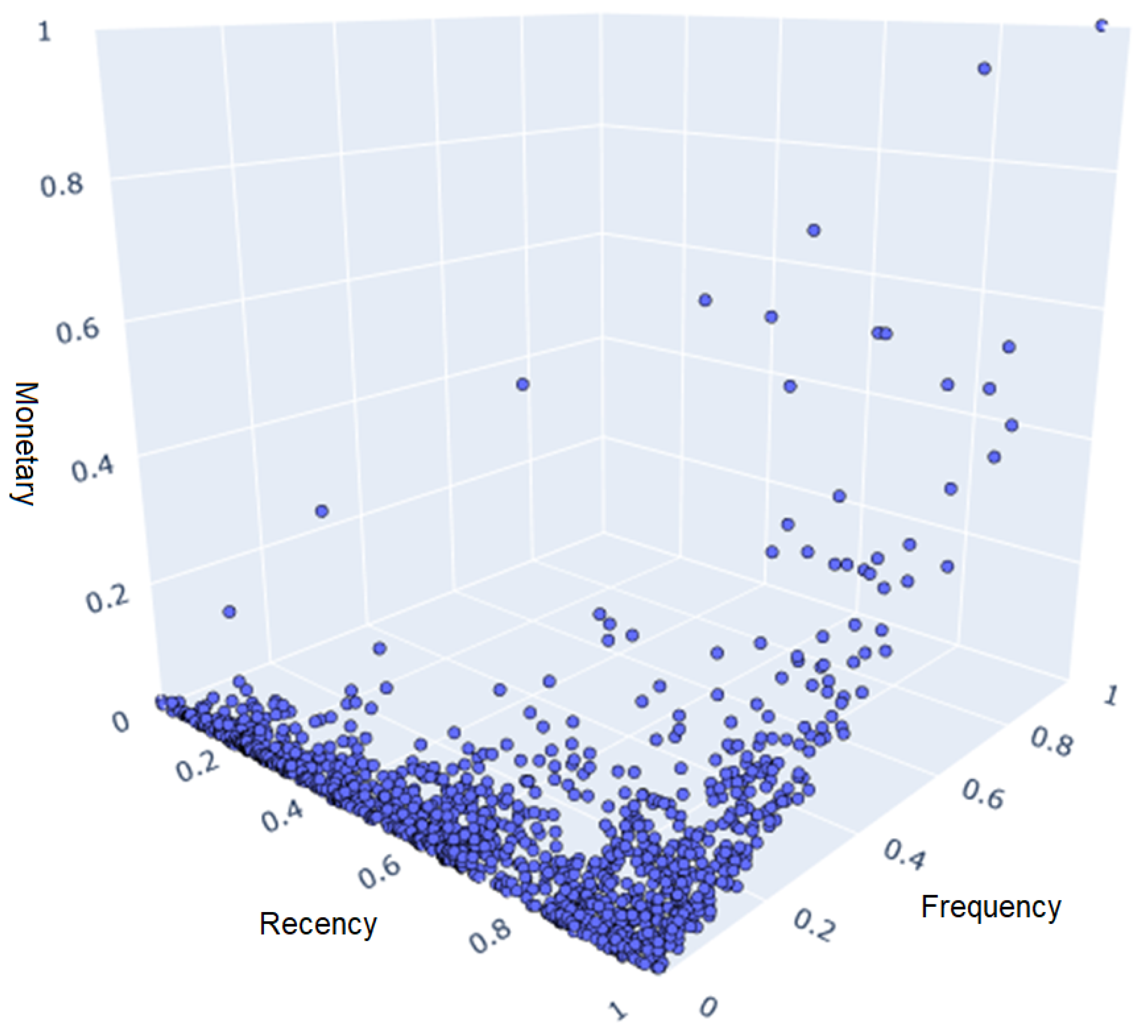
After organizing the data, it is possible to present each customer in a 3D graph, with each axis representing an attribute as in Figure 1. It is possible to identify that although the data do not provide a natural cluster distribution, it does present a structure of its own, with many customers clustered in the left corner of the graph indicating a low frequency, distributed over several recency intervals, with few high-monetary-attribute customers.

The segmentation and validation steps were performed in parallel since the algorithm used, K-means, requires the specification of the desired number of clusters. Internal and external validations were available to assist in the decision [49]. Through a statistical analysis of the 30 internal indexes researched, 10 prove to be recommendable for use. At the top of this list are the silhouette, Calinski–Harabasz, and Davies–Bouldin indexes.

To generate the silhouette index for data, only two things are needed: the clusters obtained and the set of distances between all observed data, and for each i, its respective Silhouette index $s\left(i\right)$ is calculated. The average dissimilarity of the distances of i with the rest of the data in the cluster of i, denoted by $a\left(i\right)$, is evaluated [50]. Then, the minimum value between the distances of i and any other cluster is obtained (the neighboring cluster of i is then discovered, i.e., the cluster with which i would most fit if it were not in its original cluster), denoted by $b\left(i\right)$. This process can be summarized by:

$$s\left(i\right)=\frac{b\left(i\right)-a\left(i\right)}{maxa\left(i\right),b\left(i\right)},$$

(2)

which results in a number between −1 and 1, where −1 is a bad categorization of the object i (not matching its current cluster) and 1 is an optimal categorization. To obtain the quality of the clustering in general, the average of $s\left(i\right)$ is obtained for all objects i in the dataset.

The variance rate criterion (VRC) considers the number of observations/data n and the number of clusters k. When this index is used, an attempt is made to maximize the result as the value of k is changed. The VRC index is given by:

$$VRC=\frac{BGSS}{k-1}/\frac{WGSS}{n-k}.$$

(3)

where BGSS is the between-group sum of squares that portrays the variance between clusters taking into account the distance from their centroids to the global centroid, and WGSS is the within-group sum of squares that portrays the variance within clusters taking into account the distances from the points in a cluster to its centroid [51].

The goal of the index is to define a cluster separation measure $R(S_i,S_j,M_{ij})$ that allows for the computation of the average similarity of each cluster with its most similar (neighboring) cluster, the lowest possible value would be the optimal result [52]. With $S_i$ being the dispersion measure of cluster i, $S_j$ being the dispersion measure of cluster j, and $M_{ij}$ being the distance between clusters i and j, according to:

$$R_{ij}\equiv \frac{S_i+S_j}{M_{ij}}\overline{R}\equiv \frac{1}{N}\sum _{i=1}^N{R}_i.$$

(4)

$R_{ij}$ is obtained for all clusters, that is, the ratio of inter- and intra-cluster distances between cluster i and j. After that, $R_i$ (the highest value of $R_{ij}$) is obtained by identifying for each cluster, the neighboring cluster to which it is most similar. The index itself is calculated $\overline{R}$, this being the total sum of the similarities of N clusters with their closest neighbors.

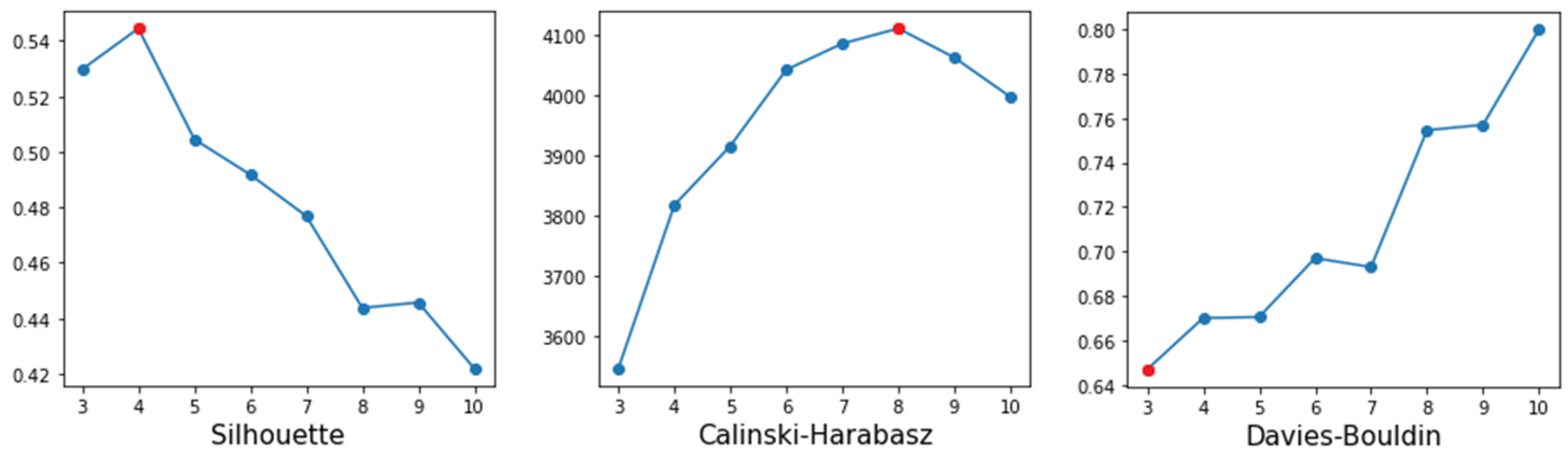
Eight segmentation solutions were generated with the K-means algorithm, starting from $k=3$ to $k=10$. After that, the best results among the k solutions according to each index were obtained. According to Figure 2, the silhouette index suggested four clusters, while Calinski–Harabasz suggested eight and Davies–Bouldin three. It should be noted that in the interpretation of the silhouette and Calinski–Harabasz index, the highest value is chosen, while in the Davies–Bouldin index, the lowest value is selected.

The suggestions for the number of clusters from the indices showed high variability, causing great uncertainty in detecting the number of clusters. This result is common among datasets that do not have naturally occurring clusters. The consumer data typically does not contain natural segments, making it difficult to obtain the optimal number of clusters from internal validation indices [40].

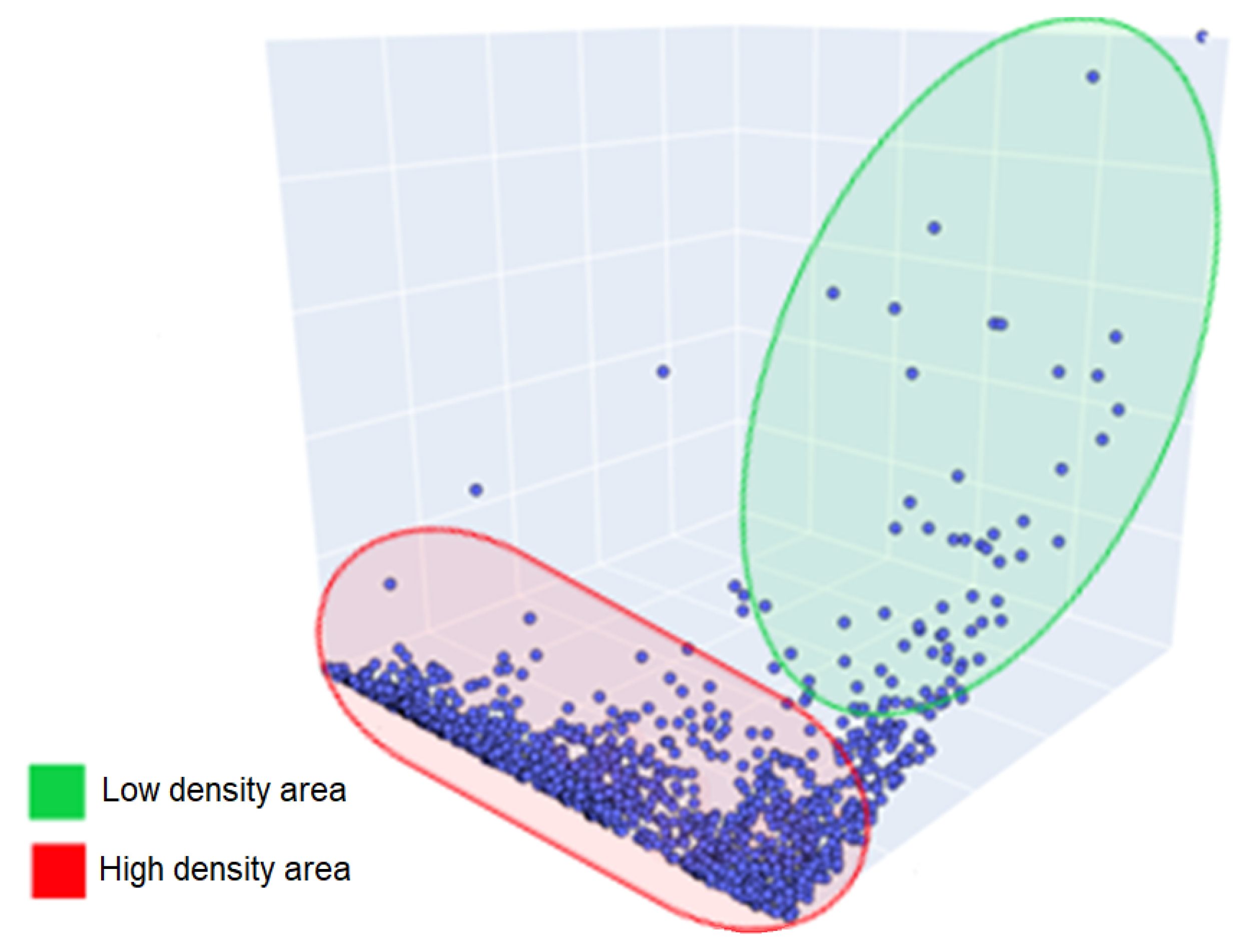
Various features in the data distribution can affect the internal validation indices. The silhouette and Davies–Bouldin indices suffer from close clusters, and Calinski–Harabasz performs poorly on unequal-size distributions [53]. All these cited characteristics are present when viewing the distribution of the data in Figure 3, which in addition to showing different sizes in the possible clusters demonstrates a clustering of data on a specific side of the distribution and a low-density in areas of a high monetary attribute.

3.3. Specification

For the description of the prototype functions, the functional requirements (FR) and non-functional requirements (NFR) are shown in

Table 4. Requirements.

Functional Requirements	RF01	Acquire the transaction data of customers from a database.
	RF02	Filter out customers with irregular information.
	RF03	Extract the characteristics used in the RFM model from the customers.
	RF04	Normalize the data to avoid disparities in attribute scales.
	RF05	Display on a 3D graph the location of the customers from the RFM feature scores.
	RF06	Segm. into clusters the cust. based on the RFM attributes.
Non- Functional Requirements	RNF01	Use the K-means clustering algorithm for segm. of clients.
	RNF02	Apply the silhouette, Calinski–Harabasz, and Davies–Bouldin internal validation indexes to val. the quality of the clusters.
	RNF03	Apply the external validation index of global stability, stability per cluster, and SLSa stability.
	RNF04	Use the Python language for prototype development.

. To obtain the customers and pertinent information from a commercial management software database. The market segment of the database in question is focused on the sale of men’s and women’s clothing. The customers were extracted with information from the considered period, which represents the structure needed to perform the segmentation based on RFM attributes.

3.4. Global Stability

With the uncertainty generated by the internal validation indexes, it is necessary to acquire other views on the dataset, so that it is possible to ensure an optimal number of clusters with an acceptable margin of certainty [54]. External validation indices were applied. Since there are no “true” clusters or test data with a priori categories to make the external comparison, a global stability measure was used, where the external information is composed of solutions with different amounts of clusters.

The external information uses the main concepts: bootstrapping for random sample selection, and the adjusted Rand index (RI) for the similarity measure between the two clustering solutions z and $z^{\prime }$. The RI can be defined by:

$$RI=\frac{a+d}{a+b+c+d},$$

(5)

where a is the number of element pairs that were assigned to the same cluster.

For that, b is the number of element pairs that were assigned to the same cluster in solution z, but in different clusters in solution $z^{\prime }$. c is the number of element pairs that were assigned to different clusters in solution z, but in the same clusters in solution $z^{\prime }$, and finally, d is the number of element pairs that are in different clusters in both z and $z^{\prime }$ [55].

The RI has some issues, such as not always presenting a value of 0 for completely random solutions and varying positively as the number of clusters in the solutions increases. Different measures have been created to correct such problems; one of these measures is the adjusted Rand index (ARI), given by:

$$ARI=\frac{Index-ExpectedIndex}{MaxIndex-ExpectedIndex}.$$

(6)

With Index being the result of RI, Expected Index being the expected RI when observations are randomly assigned to different clusters, and Maximum Index being the maximum possible value of RI. The ARI index ranges between −1 and 1, with −1 being a value for high dissimilarity and 1 being a value for high similarity between two solutions [56]. From these two concepts presented, it is possible to apply the global stability measure divided into the following steps:

(a)

Creating 50 pairs of bootstrap samples with replacements from the data;

(b)

Performing the clustering of each pair of samples with k clusters;

(c)

Calculating the ARI value of the clustered pair, generating a value from −1 to 1;

(d)

Repeating steps “b” and “c” until the desired number k is reached [54].

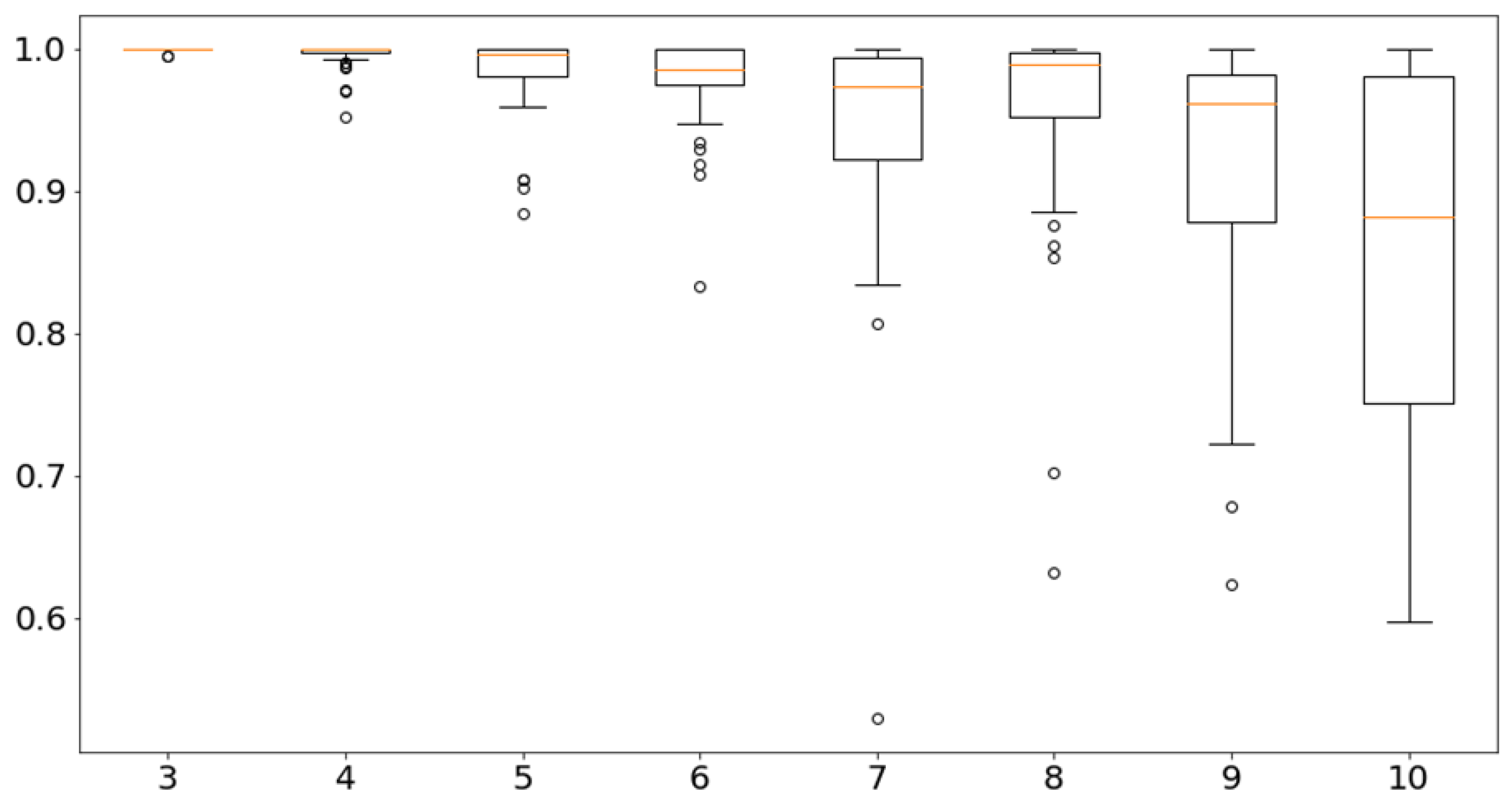
After applying ARI, 50 values are used for each k analyzed. Then, it is possible to represent the values in a boxplot chart as shown in Figure 4, where the horizontal axis represents the solutions with different numbers of clusters and the vertical axis represents the ARI index value. The box shapes represent 50% of the values and the outer dashes represent the other 50%.

Outliers are represented by circles outside the outer part, and the orange dash indicates the average of the values. With this graph, a view of the stability of each solution with k clusters is obtained. The ARI tends to decrease as k is increased, indicating a greater variation in the possible differences between the clusters of each solution.

Analyzing the boxplot, after six clusters, the ARI value between solutions constantly varies negatively. Therefore, solutions with four, five, and six clusters become viable, since they have desirable stability in relation to solutions with k larger numbers, and still, allow for a more detailed analysis of each cluster. $k=3$ was not considered because it has few clusters, aggregating different customers in the same group, making the solution more generalized and with few discernible details in each cluster.

3.5. Stability by Cluster

Global stability allows for an analysis of the solutions with respect to their change according to several executions of a clustering algorithm, but does not allow for a detailed analysis of the specific structure of the solutions, i.e., the clusters [57]. After selecting three segmentation candidates ($k=4, k=5$, and $k=6$), it is possible to calculate the cluster stability, which is similar to the previous method, but with a focus on clusters instead of entire solutions.

This stability allows for the detection of unstable clusters within stable solutions and vice versa, helping later in descriptive analyses and selection of the solutions themselves, since it provides a view by cluster, facilitating the choice of a potential customer segment. The method uses bootstrapping and Jaccard’s index to calculate stability.

The Jaccard index (J) measures the similarity between two datasets A and B, considering the union and intersection of these sets, as expressed:

$$J\left(A,B\right)=\frac{\left|A\cap B\right|}{\left|A\cup B\right|}=\frac{\left|A\cap B\right|}{\left|A|+|B\right|-\left|A\cap B\right|}.$$

(7)

The upper part represents the intersection of A with B, thus containing values common to both sets. The lower part represents the union of A with B, containing all the values of A and all the values of B, then subtracting the values common to both sets to avoid their duplication. The Jaccard index returns a value between 0 and 1, with 1 being a value that represents the similarity between the two sets, and 0 representing the total dissimilarity between the sets [58].

Through Jaccard’s index, each cluster belonging to the original solution with its bootstrap representation is compared, generating an index for each cluster. Running the algorithm results in 100 values in a range from 0 to 1 for each cluster, which can then be displayed in a boxplot. The horizontal axis of each graph represents the different clusters contained in a solution, while the vertical axis represents the value of Jaccard’s index, allowing for the intuitive visualization of the stability of each cluster within a solution.

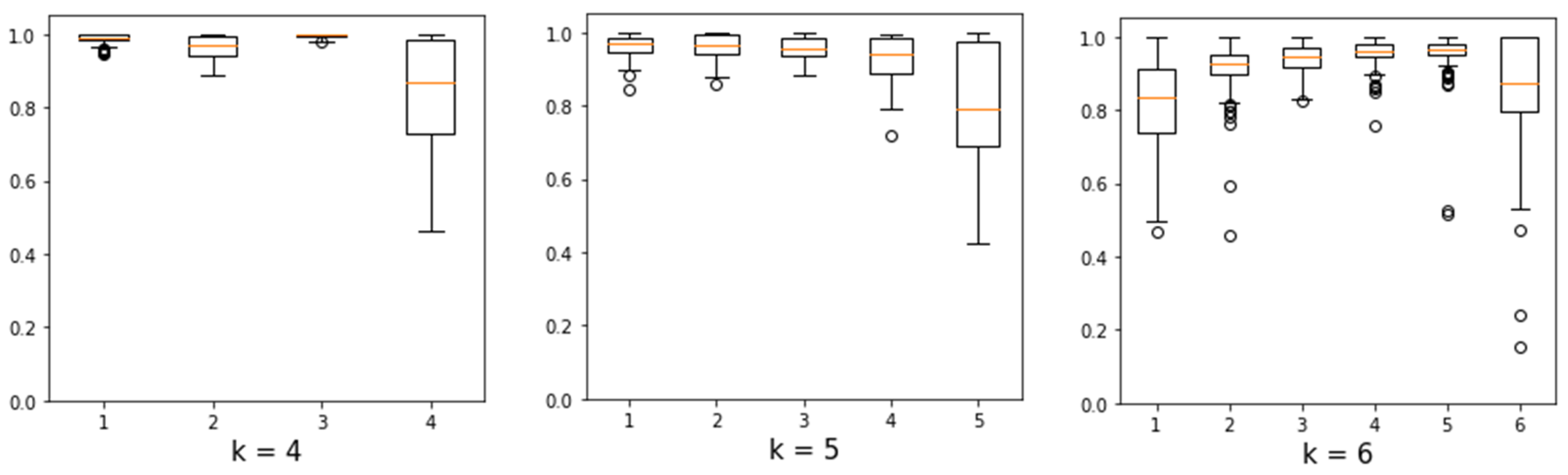
As there are three candidates for the solution ($k=4, k=5$, and $k=6$), the algorithm was applied to each one resulting in Figure 5, where it is possible to compare the solutions with respect to the stability of their clusters. It can be observed in the solutions with $k=4$ and $k=5$ that the last cluster has great instability, reaching Jaccard values close to 0.4.

In the solution with $k=6$, the stability of the last cluster varies with less intensity. The solution still presents an instability in the first cluster, indicating a possible division of a large and unstable cluster into two smaller and more stable clusters.

3.6. SLSa Stability

Another method for analyzing possible solutions with respect to the number of clusters is the SLSa, which evaluates the cluster-level stability over several solutions and allows changes in cluster structures such as joins and splits to be identified, providing information about the history of a cluster regarding its composition. This method applies the concept of relabeling and uses the entropy measure formulated by Shannon [59].

For the dataset used in this work, although the focus is on candidate solutions with $k=4$, $k=5$, and $k=6$, it was chosen to apply relabeling on solutions with $k=2$ through $k=9$ for a better understanding of the cluster formation process. The entropy represents the uncertainty in a probability distribution ($p_1,p_2,p_3,\dots ,p_k$) [60]. It is described by:

$$H=-\sum _{i=1}^n{p}_{j}log{p}_j,$$

(8)

where $p_j$ is the probability distribution in question.

The maximum entropy value consists of a probability distribution where all values are equal, resulting in an entropy value $H=1$. The minimum entropy value consists of a probability distribution where only one of the values is $1,[0,0,1,0,0]$, for example, resulting in an entropy value $H=0$, and in the context of the algorithm, signaling that all the data in one cluster in a solution are the same as all the data in another cluster in a previous solution.

To apply the SLSa, it is necessary to calculate the entropy measure H of each cluster $S_l^i$ (cluster l belonging to the solution i) with respect to all clusters of the previous solution $S_j^{i-1}$ (clusters $j=1,\dots ,k_{i-1}$ belonging to the previous solution $i-1$). Therefore, the SLSa value of a segment l belonging to a solution with $k_i$ segments is defined by:

$$SLSa\left(S_l^i\right)=-1\frac{H}{log\left(k_{i-1}\right)},$$

(9)

where a minimum value of 0 represents the worst possible stability, while 1 indicates the best possible stability. In short, a cluster with $SLSa=1$ is equivalent to a cluster that was not formed from other clusters, while a cluster with $SLSa=0$ was created from two or more clusters in the previous $k-1$ solution.

3.7. Clustering Methods

Based on the results of SLSa, the standard K-means [61] is compared to the K-medoids [62] and MiniBatch K-means [63]. Then the most appropriate clustering model is standardized for the following analyses.

3.7.1. K-Means

The K-means algorithm is a clustering technique used in data analysis and machine learning. Its goal is to partition a given dataset into K distinct, non-overlapping clusters [64]. Each data point is assigned to the cluster whose centroid (mean) is closest to it. This algorithm is particularly useful for grouping similar data points together [65]. The K-means algorithm follows a simple yet effective process:

• Initialization: Choosing K initial cluster centroids. These can be randomly selected data points or determined using other methods.
• Assignment: Assigning each data point to the nearest centroid. This creates K clusters.
• Update: Recalculating the centroids of the clusters based on the current assignment of data points.
• Iteration: Repeating the assignment and update steps iteratively until convergence. Convergence occurs when the centroids stabilize or a predetermined number of iterations is reached.

Given a dataset with N data points $\{x_1,x_2,\dots ,x_N\}$ and cluster centroids $\{c_1,c_2,\dots ,c_K\}$, the assignment step can be mathematically expressed as follows:

$$\mathrm{cluster}\left(x_i\right)=arg\underset{j}{min}\left|\right|x_i-c_j{\left|\right|}^2$$

where $\left|\right|x_i-c_j{\left|\right|}^2$ represents the squared Euclidean distance between data point $x_i$ and centroid $c_j$. The update step involves calculating new centroids $c_j$:

$$c_j=\frac{1}{N_j}\sum _{x_i\in \mathrm{cluster}\left(j\right)}{x}_i$$

where $N_j$ is the number of data points in cluster j.

3.7.2. K-Medoids

The K-medoids algorithm is a variation of the K-means clustering technique that aims to partition a dataset into K distinct, non-overlapping clusters [66]. Unlike K-means, which uses the mean (centroid) of a cluster to represent it, K-medoids employs the actual data points, known as medoids, as representatives. This makes K-medoids more robust to outliers and able to handle non-spherical clusters [67].

The procedure of K-medoids is equivalent to the K-means clustering; the difference is the evaluation of medoids [68]. Given a dataset with N data points and medoids $\{m_1,m_2,\dots ,m_K\}$, the assignment step involves selecting the medoid that minimizes the dissimilarity:

$$\mathrm{medoid}\left(x_i\right)=arg\underset{j}{min}\mathrm{dissimilarity}(x_i,m_j).$$

The dissimilarity function can be defined based on a suitable distance metric [69], such as the Euclidean distance. The update step aims to find the best medoid replacement for each cluster:

$$m_j^{\prime }=arg\underset{x_i\in \mathrm{cluster}\left(j\right)}{min}\sum _{x_k\in \mathrm{cluster}\left(j\right)}\mathrm{dissimilarity}(x_k,x_i).$$

3.7.3. MiniBatch K-means

The MiniBatch K-means algorithm is a variation of the K-means clustering technique designed to efficiently handle large datasets [70]. While standard K-means can be computationally expensive for sizable datasets, MiniBatch K-means offers a more scalable approach by using random subsets (mini-batches) of data for each iteration. This accelerates the convergence process and reduces memory requirements.

Since the algorithm uses mini-batches, it introduces some level of randomness in each iteration. This might lead to suboptimal results if not managed properly. The quality of clusters might vary depending on the mini-batch sizes and the initialization strategy. The core mathematical formulation of MiniBatch K-means remains similar to the standard K-means algorithm, with the main differences in the assignment and update steps, which are performed on mini-batches [71].

4. Results and Discussion

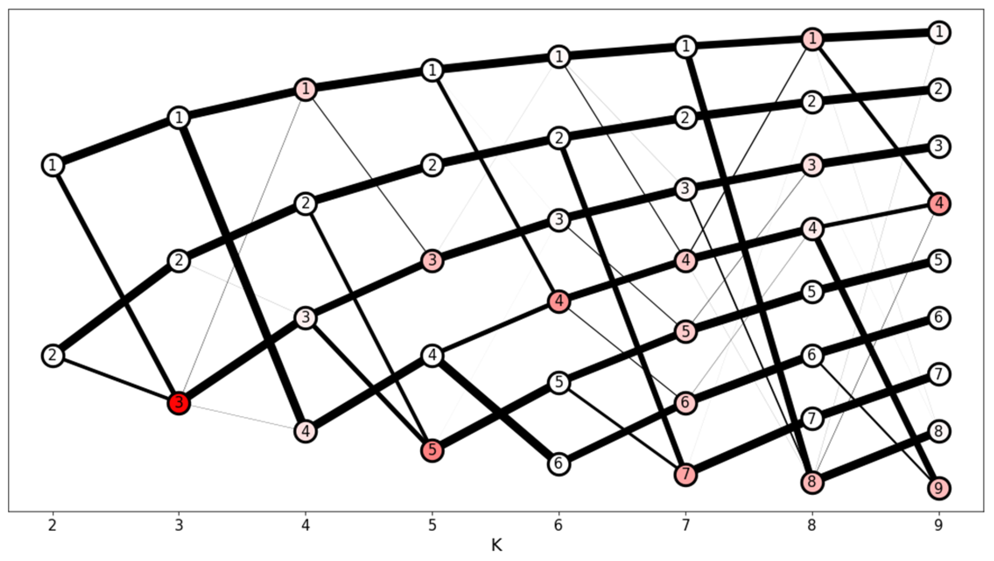
This section presents the results and discussions concerning the application of the proposed method, considering the initial calculations to define the stability criteria. After calculating the SLSa for each cluster of each solution up to $k=9$, it is possible to represent the values in a graph (see Figure 6), starting from a solution with two clusters in the left corner and ending with a solution with nine clusters in the right corner. Clusters with low SLSa values are colored with a shade of red according to their instability.

In Figure 6, the black lines represent the number of clients belonging to one cluster that is assigned to another cluster in the next solution; thick lines indicate a larger amount, and many lines to the left of a cluster indicate that it was generated from several others.

Cluster number 3 in the three-cluster solution has a high level of instability since it was created from the data in clusters 1 and 2 in the previous solution (effectively representing half of each cluster in the previous solution). Other clusters follow the same behavior: more specifically, the clusters created from a new solution (the last clusters in each column) are most often the product of joining parts of other clusters.

After solution 6, almost all the clusters in the following solutions present some amount of instability, being formed from two or more clusters in previous solutions with a few exceptions. Of the candidate solutions (4, 5, and 6) only solution 6 presents a satisfactory distribution of stable clusters, with five clusters having only one parent in the previous solution.

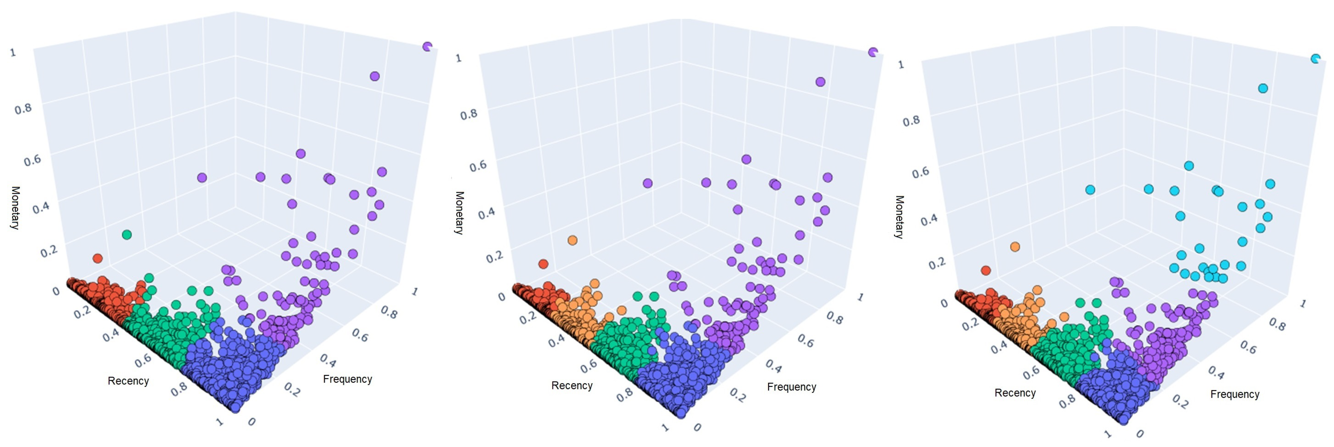
For better visualization, Figure 7 shows the transition of clusters along the different candidate solutions. Cluster 5 (in orange) was created in solution 5 from data coming from clusters 2 (in red) and 3 (in green). Similarly, cluster 6 (in cyan) in solution 6 was created from half of the data from cluster 4 (in purple), which consequently was shifted towards cluster 1 (in purple), resulting in the apparent “junction” between two halves of clusters.

Customers in cluster 6 (in cyan) are completely absorbed into another cluster in the smaller solutions, despite having unique characteristics such as having all three RFM attributes high compared to the rest of the clusters. Therefore, the solution with six clusters was chosen because it satisfactorily represents all customer types present in the dataset, as well as having an acceptable overall stability (above 0.95) and a tolerable instability per cluster (only one cluster formed from shifts).

4.1. Comparison to Other Algorithms

When applying K-medoids and MiniBatch K-means to the same database, there were variations from the standard K-means, which will be explained here. With internal indices, there was a recommendation of four clusters by the silhouette index, eight or nine clusters by the Calinski—Harabasz index, and three clusters by the Davies—Bouldin index. In this case, the internal validation indexes did not provide an equivalent value in the number of clusters. Therefore, unlike the result of standard K-means, K-medoids, and MiniBatch K-means performed lower overall stability starting at four clusters. For standard K-means, stability remained high until solutions with six clusters.

The lower stability in other algorithms occurs because they suffer more from the repeated iterations and initializations required by stability methods. For example, K-medoids takes as centroids the very points present in the dataset and may suffer multiple divergences over too many runs of the algorithm, because as the dataset presents many points, the initialization and subsequent execution may vary.

In the case of MiniBatch, the algorithm randomly obtains a subset of the data to perform cluster assignment, further increasing the variability between solutions and contributing to lower overall stability. With the overall stability reduced, the stability per cluster follows this trend, showing more variation in most solutions. Considering K-medoids and MiniBatch K-means, there were few clusters that remain with high stability across all solutions.

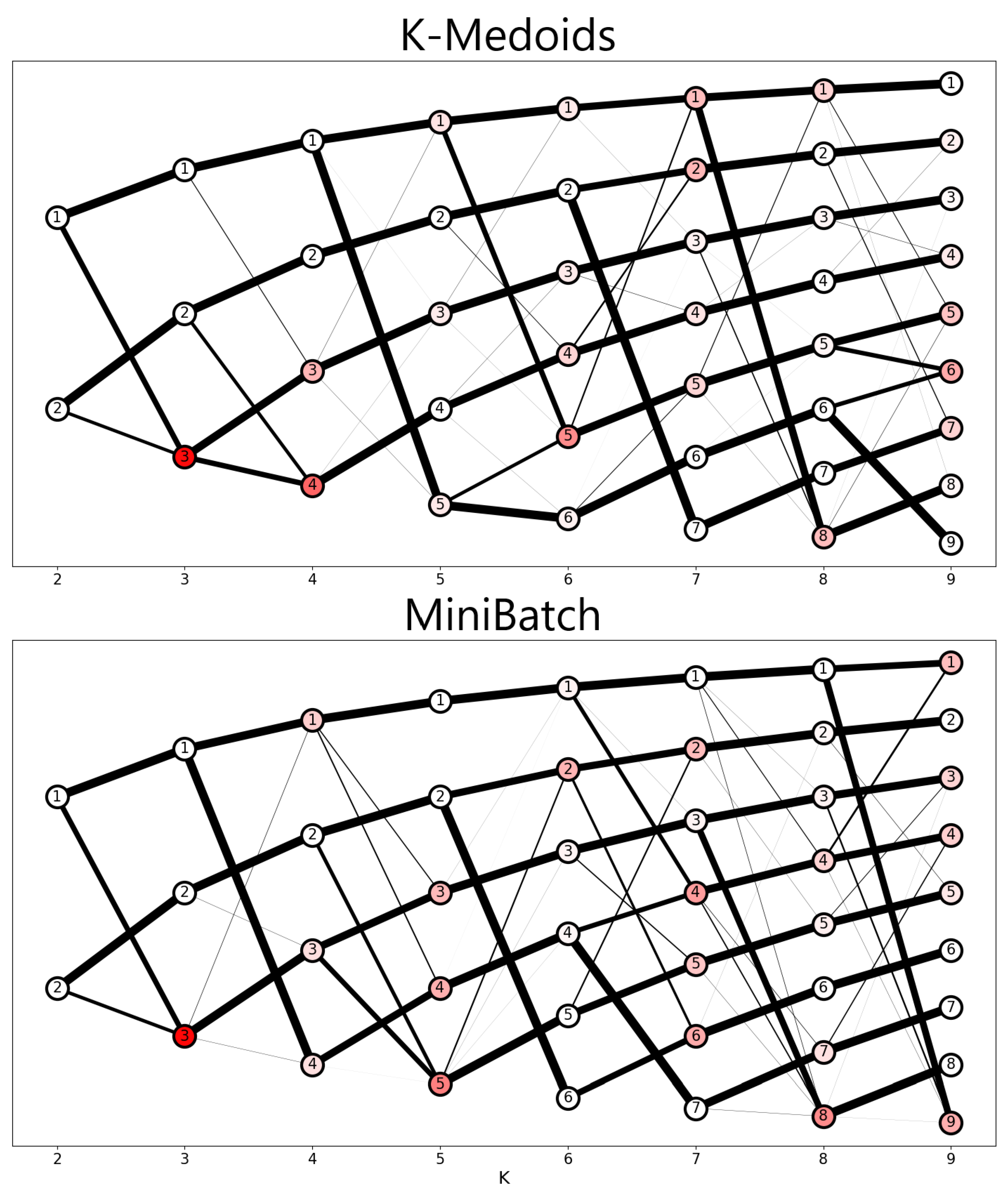
The SLSa results presented in Figure 8 show the stability drop by demonstrating the history of each cluster in each solution. Note that in comparison with the result referring to K-means (Figure 6), the two algorithms presented many more “Splits” and “Joins” among the members of each solution, contributing to a larger number of clusters with an inadequate entropy level, while K-means exhibits this behavior only after the amount of six clusters.

The external validation indexes prove to be not only a promising tool for choosing the number of clusters but also for comparing different clustering algorithms. Overall, K-means demonstrated higher reliability compared to K-medoids and MiniBatch K-means, showing higher stabilities throughout the analysis process.

4.2. Cluster Profile

Once the desired solution is obtained, it is necessary to analyze the clusters contained therein, so that their profile is easily understood; and which characteristics are really relevant. Witschel, Loo, and Riesen [72] state that before benefiting from the results, an analyst needs to understand the essence of each cluster, that is, what are the characteristics shared among the customers of a cluster that differentiate them from others.

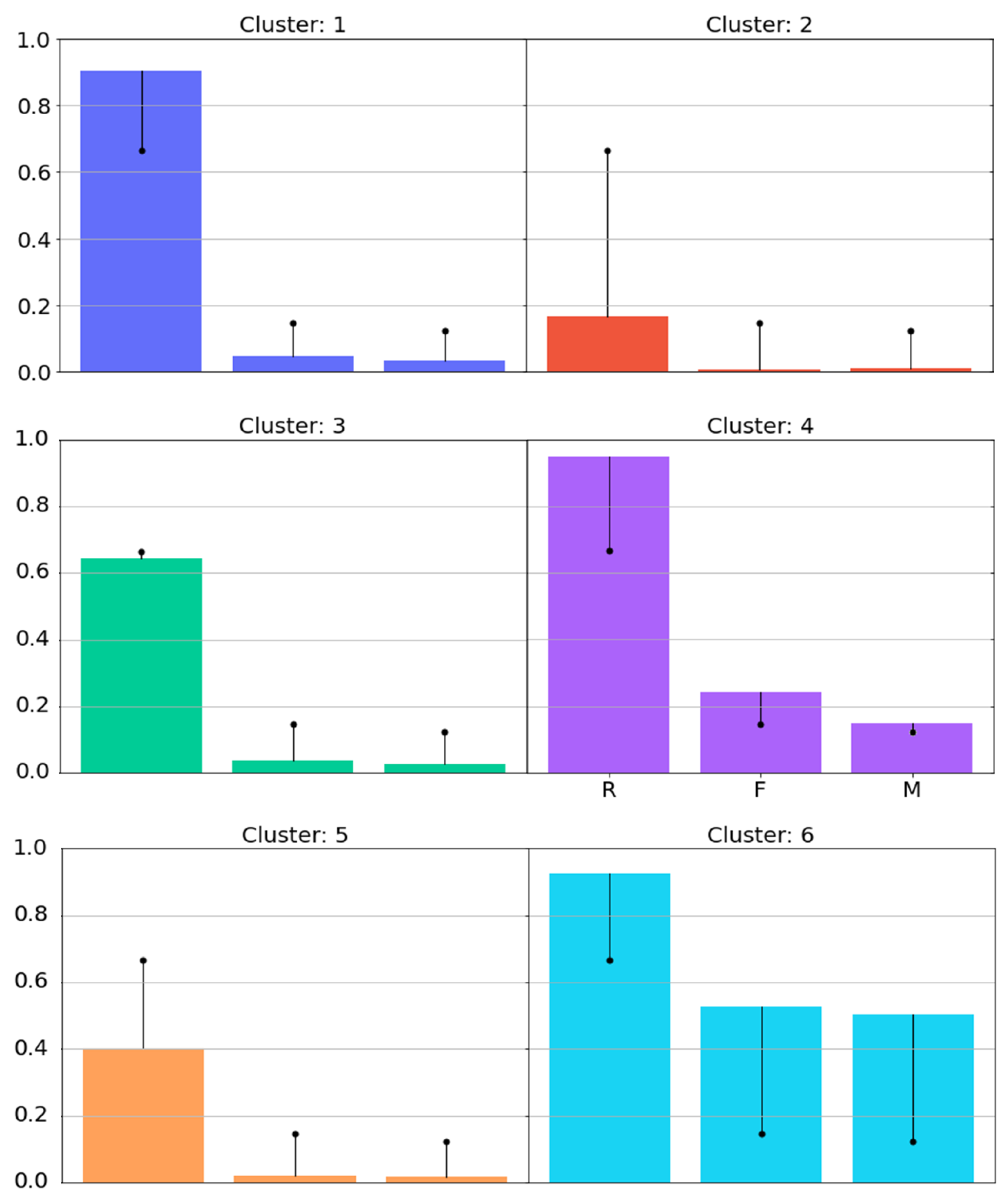
A bar chart was created that presents the average of each RFM characteristic of each cluster contained in the $k=6$ solution, presented in Figure 9. Each bar represents an RFM attribute, and its height is defined by the average of the attribute in question in the cluster. In this representation, each attribute has a black dot referring to the average of the entire solution, allowing you to compare whether the attribute of the cluster stands out in relation to all the others.

By analyzing Figure 9 considering each RFM attribute, it is possible to have the following interpretations:

(a)

Clusters 2 and 5 have a recency, frequency, and monetary attribute below the overall average, possibly indicating a type of customer who no longer frequents the store (cluster 2) or is in the process of stopping frequenting (cluster 5). Clusters 2 and 5 have 390 and 338 customers, respectively, representing about 41% of all registered customers;

(b)

Clusters 1 and 3 have high recency, but low frequency and monetary, indicating a new type of customer who is not yet familiar with the store, or is in the process of developing a frequent visiting relationship, or even an old customer who frequented the store recently. Either way, these clusters may represent the flow of customers who have recently purchased from the store. Clusters 1 and 3 have 474 and 379 customers respectively, representing about 48% of all registered customers;

(c)

Clusters 4 and 5 have above-average RFM attributes, indicating loyal customers who buy frequently and spend high total money relative to others. Cluster 6 has the highest values among all clusters, representing the store’s best customers. Its RFM attributes are expressively higher, yet this cluster contains only 28 customers. Cluster 4 also has fewer customers than the other clusters, with 139 in total. The two clusters together represent a total of 167 customers, about 11% of all registered customers.

With the information generated by the cluster profiles, it is possible to obtain a succinct summary of the types of customers who frequent the company, these being lost customers (with low recency, frequency, and monetary), customers in the process of being lost (with below-average recency; low frequency and monetary), recent customers (with high recency but low frequency and monetary), less recent customers (with high recency but lower than recent customers, and a lower frequency and monetary than recent customers), loyal customers (high recency, frequency, and monetary), and finally, the best customers (the best possible RFM attributes).

4.3. Cluster Description

From the analysis of segmentation variables, it becomes feasible to implement promotional campaigns, incentive actions, and even methods to rescue lost customers. However, the analysis is not necessarily finished; one of the important steps after obtaining the cluster profiles is the description process. Cluster description consists of the individual analysis of the clusters from variables external to the clustering process, called descriptive variables [40]. These variables can contain information from questionnaires, and other characteristics pertinent to the scope of the company.

As the database has a large amount of eligible information, five were chosen for the cluster description process: age, sex, time of contact with the store, number of purchases per season, and rate of returns. After extracting the descriptive data, mosaic charts were used for display. This type of chart is similar to a bar chart but displays the information in cells that have their size relative to the amount of information observed and may vary in width according to the number of customers/purchases in a cluster, and in height according to the percentage of the variable observed compared to the percentage of other variables.

Another concept pertinent to the mosaic chart is the statistical model applied, called bimodal distribution, which displays abnormal variations in the distribution of values based on an assumption of independence of variables. In this way, higher-than-expected values (above two standard deviations, or outside the 95% value limit) are displayed in red shades of greater intensity, lower-than-expected values are displayed in blue shades of greater intensity, and normal values take on green. With this view, it is possible to observe unique characteristics of clusters that have abnormal variations.

Regarding the descriptive information used, the age variable was transformed into an ordinal variable. This variable starts from 18 to 24 years old, considering age intervals of six years onwards for each category, with the penultimate one being for customers over 40 years old and the last one for a category representing a lack of information in the register. The gender variable available in the database consists of the categories “male” and “female”.

The result of the graphs applied to these variables can be seen in Figure 10, which presents the age graph on the left side and the sex graph on the right side; each graph displays on the vertical axis the categories of the descriptive variables analyzed and on the horizontal axis the clusters. Since the distribution of the cells occurs according to the observed variable and the number of observations in the cluster, the size of each varies in width and height. Taking cluster 6 (C6) as an example, its width is thin due to the low number of customers it has, and the height of each cell belonging to it depends on the percentage that each category represents in relation to the other categories in the same cluster; if a category has 99% of customers, it will occupy 100% of the cell, as in cluster 6 (C6) in the graph on the right side.

By analyzing Figure 10, it is possible to have the following interpretations:

(a)

Regarding age (left graph), the cluster of recent customers (C1) has a lower-than-expected number (cells in blue) of adult and elderly customers and higher concentrations of young adults and customers with no information, indicating that there may be a flow of young people being attracted by the store. The cluster of lost customers (C2) has a higher-than-expected number of customers who did not inform their age, indicating a certain resistance to filling out registrations. The cluster of customers being lost (C5) has a higher-than-expected number of customers over 30 years old, indicating a possible dissatisfaction with the products offered to this age group, information that is corroborated by the fact that the flow of recent customers (C1) has more young people than expected.

(b)

Regarding gender (right chart), the most important customers (belonging to clusters C4 and C6) are mostly women and are in larger numbers than expected, even though the store offers male lines, indicating a female preference for the clothes offered. This information is corroborated by the fact that the clusters with customers lost or in the process of being lost (C2 and C5) have a larger number of men than women, indicating a possible lack of male engagement with the options offered.

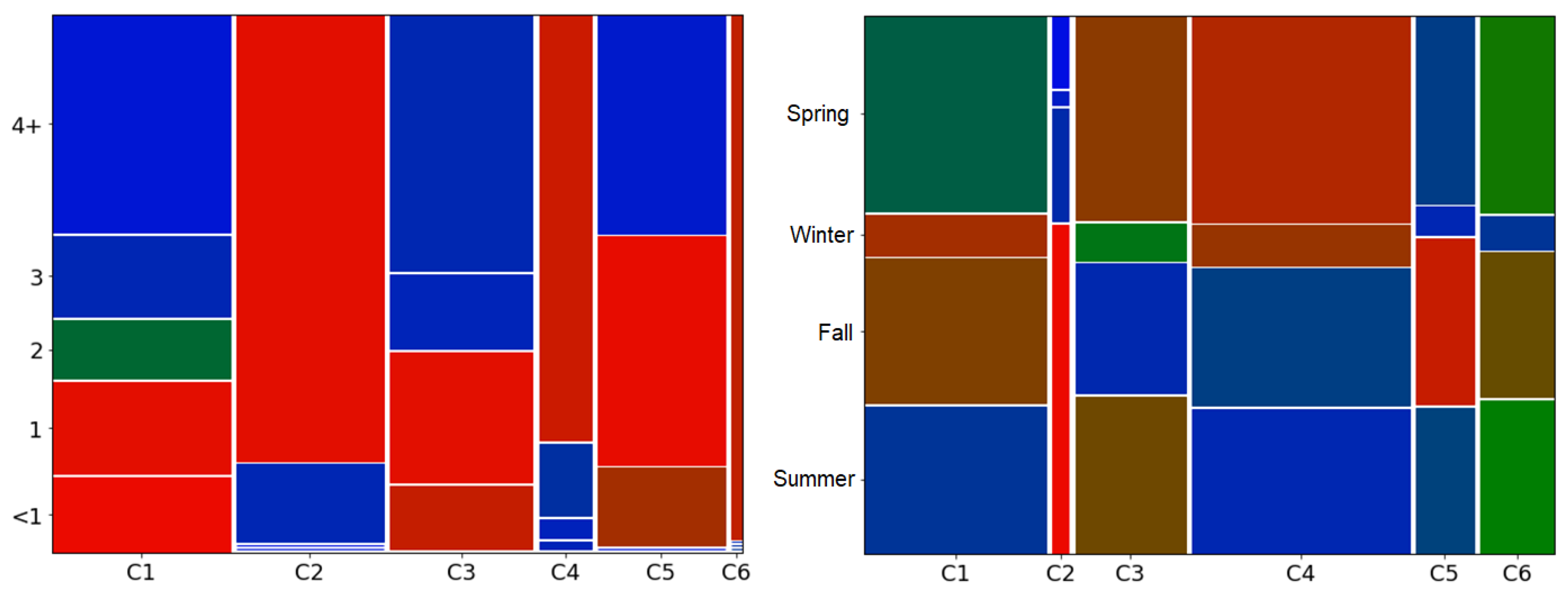
The two other variables that allow for a mosaic display are the number of years since a customer’s registration with the company and the number of purchases made during each season. For the first, the intervals were established as less than a year (<1), one, two, three, and more than four years. For the second, the intervals are composed of the four seasons (summer, autumn, winter, and spring). The graphs generated are shown in Figure 11, which follows the same structure as the previous figure.

From the analysis of Figure 11, it is possible to make the following interpretations:

(a)

In relation to the time of customers’ registration (graph on the left side), it is possible to identify that the clusters with recent customers (C1 and C3) have a higher number of newly registered customers than normal, as well as customers with one year of registration, allowing one to identify that these clusters present a flow of new customers. The clusters with the best customers (C4 and C6) have many customers registered for more than four years (in cluster C6 it is all customers), indicating that customers with an acceptable RFM performance are rarely new customers, requiring a long relationship with the store. Finally, clusters C2 and C5, which represent customers lost or in the process of being lost, present many customers registered for more than four years, which justifies the characteristic of lost customers.

(b)

Regarding the number of purchases per season (right chart), the chart shows the preferences of each cluster in relation to specific seasons, showing a general preference for the winter, summer, and fall collections. The cluster of lost customers (C2) shows a high rate of purchases made during the summer, possibly indicating a certain dissatisfaction with this season’s line, since customers in this cluster no longer frequent the store. The cluster with the second-best RFM performance (C4) presents the highest number of purchases of all the other clusters (denoted by the width of the cells); of these sales, higher than normal was the frequency of purchases in spring, indicating a preference of this group for the line of this season.

The last variable analyzed, purchase returns rate (transaction or sale that contains at least one return), was obtained through the ratio between the number of returns in a cluster and its total sales quantity. Thus,

Table 5. Rate of returns per cluster.

Clust. 1	Clust. 2	Clust. 3	Clust. 4	Clust. 5	Clust. 6
9.09%	6.93%	8.11%	11.81%	8.68%	17.50%

displays the percentages of returns for each cluster.

Based on the percentages presented, the clusters with the best RFM performance (clusters 4 and 6) have the highest return rates (11.81% and 17.50% respectively), indicating a high selectivity among their customers. The cluster of lost customers (cluster 2) has the lowest return rate (6.93%), indicating that a dissatisfied customer rarely makes a return, and simply does not frequent the store anymore instead of exchanging the product and trying to buy again.

5. Conclusions

Customer segmentation allows for an in-depth analysis of a company’s customer behavior. With the right data, previously obscure profiles can be identified, based on information sometimes considered useless beyond the operational layer of a company’s sales and registration. This work had as its initiative the numbering and identification of these profiles, for which the database of a real retail clothing company was used, containing registration and transaction information from 1845 customers. Each customer was assigned characteristics based on the RFM model, and then the data were cleaned and manipulated to fit the clustering algorithm used (K-means).

To validate the cluster solution as well as its quantity, three internal validation indexes were used, and when they were not conclusive enough to define the quantity, the following external validation indexes were used: a global stability measure based on the ARI index, a stability measure per cluster based on the Jaccard index, and the SLSa method from the entropy measure. After selecting three candidate solutions (with four, five, and six clusters) based on global stability; the stability per cluster presented a better result in the solution with six clusters, then being confirmed and detailed from the SLSa method, demonstrating the process of dividing and joining clusters throughout the iterations with different numbers for the k parameter of the K-means algorithm.

Thus, the solution with six clusters was chosen, and its clusters were presented in a chart containing their RFM characteristics so that their profiles could be detected based on inferences made from their attributes. With the profiling of the clusters, six segments were named based on their peculiarities: lost customers (with low recency, frequency, and monetary), customers in the process of being lost (with below-average recency; low frequency and monetary), recent customers (with high recency, but low frequency and monetary), less recent customers (with high recency, but lower than recent customers, and a lower frequency and monetary than recent customers), loyal customers (high recency, frequency, and monetary), and finally, the best customers (best possible RFM attributes).

After highlighting the profile of each segment through the RFM segmentation variables, an analysis was performed from descriptive variables based on the data available in the database. The segments were evaluated through mosaic graphs and tables based on their age, gender, registration time, purchases per season, and returns, and particularities present in each descriptive variable were pointed out, such as possible trends of the segments, abnormal flows, and non-standard amounts, among others.

The objective of identifying different customer segments based on their behavior was achieved. Although the internal validation indexes do not present a consensus among the number of natural clusters, it was possible to obtain a guarantee of the stability of the segments through the external indexes. That said, it is clear that despite the absence of natural clusters, it was still possible to obtain significant segments, containing distinguishable characteristics that differentiate them from each other, allowing for further insights into the types of customers who frequent the establishment, extrapolating to customer types in general in the retail industry.

Furthermore, this work contributes to the academic community, by applying models (RFM), indexes (three internal and three external), methods (Min-Max normalization, bootstrapping, Jaccard Index, and ARI), and the K-means algorithm in a real database, analyzing its influence on data with a different distribution of training data (whose characteristics commonly present well-defined clusters, unlike a database with real data). A conclusion derived from applying such techniques to this dataset is that internal validation indices do not always present a consensus on the number of clusters requiring the use of other types of validation.

Valuable information for the apparel retail industry and possibly other industries can be extracted from a database of transactional and registration information, indicating the intrinsic value of data that is often only stored and rarely analyzed in the context of customer clusters. The proposed approach presented in this paper could be applied to other databases, helping decision making based on extra information from the data. Since the proposed method needs to have a convex-shaped cluster when other shapes are evaluated, the proposed method could not be the best alternative. In this case, other clustering methods such as the DBSCAN may be the best approach.

Given the above, the present work can be complemented by the following proposals: the use of the RFM method in conjunction with K-means applied to a database of a different retail branch, such as supermarkets, dealerships, and real estate agents, among others; the application of different internal and external indexes for the validation of the quality of clusters under different visions; the use of other descriptive variables, such as time spent per purchase, lines of products most purchased, and quantity of products per purchase; the application of questionnaires, to use in conjunction with the analysis of the profiles, crossing the variables based on the questioned cluster.