Article

Bundle Enrichment Method for Nonsmooth Difference of Convex Programming Problems

1
DIMES (Dipartimento di Ingegneria Informatica, Modellistica, Elettronica e Sistemistica), Università della Calabria, 87036 Rende, CS, Italy
2
School of Mathematical Sciences, RMIT University, Melbourne 3000, Australia
3
Centre for Smart Analytics, Institute of Innovation, Science and Sustainability, Federation University Australia, Ballarat 3350, Australia
4
Department of Computing, University of Turku, FI-20014 Turku, Finland
*
Author to whom correspondence should be addressed.
Algorithms 2023, 16(8), 394; https://doi.org/10.3390/a16080394
Submission received: 2 August 2023 / Revised: 18 August 2023 / Accepted: 19 August 2023 / Published: 21 August 2023

Abstract

:
The Bundle Enrichment Method (BEM-DC) is introduced for solving nonsmooth difference of convex (DC) programming problems. The novelty of the method consists of the dynamic management of the bundle. More specifically, a DC model, being the difference of two convex piecewise affine functions, is formulated. The (global) minimization of the model is tackled by solving a set of convex problems whose cardinality depends on the number of linearizations adopted to approximate the second DC component function. The new bundle management policy distributes the information coming from previous iterations to separately model the DC components of the objective function. Such a distribution is driven by the sign of linearization errors. If the displacement suggested by the model minimization provides no sufficient decrease of the objective function, then the temporary enrichment of the cutting plane approximation of just the first DC component function takes place until either the termination of the algorithm is certified or a sufficient decrease is achieved. The convergence of the BEM-DC method is studied, and computational results on a set of academic test problems with nonsmooth DC objective functions are provided.

1. Introduction

Optimization approaches are essential for solving a wide range of practical problems. There are various problems based on these approaches including unconstrained and constrained problems, problems with linear and nonlinear as well as smooth and nonsmooth objective and/or constraint functions, and problems with continuous and integer decision variables [1]. The majority of optimization problems from applications have special structures (for example, convexity) which can be exploited to design efficient and accurate methods for their solutions. Difference of convex (DC) optimization problems are among such problems, where the objective and/or constraint functions are represented as a difference of two convex functions.
In this research work, we consider the unconstrained nonsmooth DC programming problem
min x R n f ( x ) ,
where f : R n R is, in general, nonsmooth and is expressed as a difference of two convex functions f 1 , f 2 : R n R :
f ( x ) = f 1 ( x ) f 2 ( x ) .
Here, f 1 f 2 is called a DC representation (decomposition) of f while f 1 and f 2 are DC components of the function f . The DC components f 1 and f 2 are, in general, nonsmooth [2,3,4,5].
Nonsmooth DC programming is an important subclass of DC optimization problems [6], and many practical problems are modeled as a DC programming problem. They include the bridge location problem, the design centering problem [7], the packing problem [8], the production–transportation planning problem [9], the location planning problem [10], the edge detection problem [11], the conic programming problem [12], cluster analysis [13], and regression analysis [14]. Recently, DC optimization problems with uncertain data has become an interesting topic, and the results from robust optimization, in particular those obtained in [15,16,17], can be extended to robust DC optimization.
DC optimization problems have been studied in the context of both local and global problems, and various methods have been developed for solving these problems globally [7,18]. To the best of our knowledge, the first local search algorithm for solving DC optimization problems is the difference of convex algorithm (DCA) introduced in [19] and further explored, for example, in [8,20]. Since then, the development of local DC optimization methods for solving Problem (1) has attracted remarkable scholarly attention. Next, we provide a short description of such methods and give references for more details. These methods can be classified into three categories:
  • The first category consists of the DCA and its modifications. The basic idea of the DCA is to linearize the concave part f 2 around the current iterate by using its subgradient while keeping the convex part f 1 as it is in the minimization process. To improve the convergence of the DCA, various modifications have been developed, for instance, in [21,22,23]. The boosted DC algorithm (BDCA), proposed in [21,22], accelerates the convergence of the DCA by using an additional line search step. The inertial DCA, introduced in [23], defines trial points whose sequence of functional values is not necessarily monotonically decreasing. This controls the algorithm from converging to a critical point that is not d-stationary. In [24], the BDCA is combined with a simple derivative-free optimization method. This allows one to force the d-stationarity (lack of descent direction) at the obtained point. To avoid the difficulty of solving the DCA’s subproblem, in [25], the first DC component is replaced with a convex model, and the second DC component is used without any approximation;
  • The methods in the second category, which we refer to as DC-Bundle, are various extensions of the bundle methods for convex problems. The piecewise linear underestimates or subgradients of both DC components are utilized to compute search directions. The methods include the codifferential method [26], the proximal bundle method with the concave affine model [27,28], the proximal bundle method for DC optimization [29,30], the proximal point algorithm [31], the proximal linearized algorithm [32], the double bundle method [33], and the nonlinearly constrained DC bundle method [34];
  • The methods in the third category are those that use the convex piecewise linear model of the first DC component and one subgradient of the second DC component to compute search directions at each iteration [35,36]. They differ from those in the first category as at each iteration of these methods, the model of the first DC component is updated and the new subgradient of the second component is calculated. They also differ from those in the second category as they use only one subgradient of the second DC component at each iteration whereas the DC-Bundle methods may use more than one subgradient of this component to build its piecewise linear model. Note that some overlapping is unavoidable when classifying methods into different categories: for instance, the proximal bundle method for DC optimization [30] may be classified into both the second and the third categories. The other methods in the third category include the aggregate subgradient method for DC optimization [35] and the augmented subgradient method [36]. In the former method, the aggregate subgradient of the first DC component and one subgradient of the second component are utilized to compute search directions. In the latter method, augmented subgradients of convex functions are defined and used to model the first DC component. Then, this model and one subgradient of the second DC component are used for computing search directions.
The proposed BEM-DC method belongs to the DC-bundle family whose main features, with respect to the DCA, are
  • developing a model function based on cutting-plane approximations of f 1 and, possibly, f 2 ;
  • adding a regularization term (typically a proximity one) to the model for stabilization purposes.
We assume the familiarity of the reader with the basic notions of bundle methods. We refer to the following books and articles from the vast literature available [37,38,39,40,41,42,43,44,45]. In our iterative scheme, we adopt two cutting-plane approximations (based, as usual in bundle methods, on information coming from previous iterations) for f 1 and f 2 , respectively. Consequently, we have a model which is still DC, being the difference of two convex piecewise affine functions. Similarly to  [29,33], we tackle the (global) minimization of the model by solving a set of convex problems whose cardinality depends on the number of linearizations adopted to approximate the function f 2 . The novelty of the approach consists of the dynamic management of the bundle. This enables us to achieve a parsimonious use of the information available, in view of reducing the computational burden to minimize the model function at each iteration. The adopted strategies are based on the following:
  • The information coming from the previous iterates contributes to the approximation of exactly one of the DC components f 1 and f 2 , depending on the sign of the linearization error relative to the current iterate. During the iterative process, every time a new point is generated, subgradients of both component functions f 1 and f 2 are calculated, but only one of them will enter the calculation of the search direction: the choice being driven, at each of the successive iterations, by the sign of the linearization error with respect to the current point. Such sign may change at each iteration. Therefore, we define a dynamic bundling strategy, which implies a consistent reduction (approximately one-half) of the size of the auxiliary problems to be solved;
  • If the displacement suggested by the model minimization provides no sufficient decrease of the objective function (the null step in bundle parlance), the temporary enrichment exclusively of the cutting-plane approximation of f 1 takes place.
Note that a significant difference between the proposed approach with those introduced in [29,33] is in the reduction of the size of the bundle of the function f 2 . This has a strong impact on the solution of the auxiliary problem to be solved at each iteration.
The structure of the paper is organized as follows. Section 2 provides necessary notations and some preliminaries. Section 3 presents the new model function formulation. Section 4 describes the new method, and its convergence is discussed in Section 5. Section 6 reports the results of numerical experiments. Section 7 provides some concluding remarks.

2. Notations and Background

First, we provide some notations and definitions that we will use throughout the paper. The inner product in R n is u , v = i = 1 n u i v i , and · is the associated norm. For x R n and ε > 0 , B ( x ; ε ) is an open ball of the radius ε > 0 centered at x. The function f : R n R is locally Lipschitz continuous on R n if for every x R n , there exists a Lipschitz constant L > 0 and ε > 0 such that | f ( y ) f ( z ) | L y z for all y , z B ( x ; ε ) .
For a convex function f : R n R , its subdifferential at a point x R n is [38,41]
f ( x ) = ξ R n : f ( y ) f ( x ) ξ , y x for all y R n ,
and for ε > 0 , its ε -subdifferential is
ε f ( x ) = ξ ε R n : f ( y ) f ( x ) ξ ε , y x ε for all y R n .
Each vector ξ f ( x ) ( ξ ε ε f ( x ) ) is called a subgradient ( ε -subgradient) of f at x.
A point x * R n is called a critical point of Problem (1) if
f 1 ( x * ) f 2 ( x * ) ,
and a point x ¯ * R n is said to be an ε -critical point if [31]
ε f 1 ( x ¯ * ) ε f 2 ( x ¯ * ) .
Next, we recall the basic idea of the standard cutting-plane model for any convex nonsmooth function f . Let x k R n be the current iteration point, x j R n be some auxiliary points (from past iterations), ξ j f ( x j ) be the subgradients of the function f computed at the point x j R n for j J k , and J k is a nonempty subset of { 1 , , k } . The cutting-plane model for the function f can be given by
f ^ k ( x ) = max j J k f ¯ j ( x ) ,
where f ¯ j ( x ) = f ( x j ) + ξ j , x x j . The linearization error
α j k = f ( x k ) f ¯ j ( x k ) for all j J k
defines how well f ¯ j approximates the function f at the current iteration point x k .
In this paper, we assume that f is the DC function, and due to the lack of its convexity, the straightforward application of the cutting-plane approach is meaningless. Nevertheless, it can be separately applied to model the DC components f i , i = 1 , 2 . Thus, we have
f ^ i k ( x ) = max j J k f i ( x j ) + ξ i , j , x x j for x R n .
Here, ξ i , j f i ( x j ) , i = 1 , 2 are the subgradients of the DC components f i computed at the auxiliary point x j R n for j J k . This approximation can be rewritten as
f ^ i k ( x ) = max j J k f i ( x k ) + ξ i , j , x x k α i , j k ,
where x k R n is the current iteration point, and α i , j k , i = 1 , 2 are the linearization errors associated with the j-th first order expansion of f i , i = 1 , 2 rooted at the point x j , given by
α i , j k = f i ( x k ) f i ( x j ) ξ i , j , x k x j for all j J k .
Suppose that information coming from some auxiliary points x j R n , j J k , along with x k , ξ 1 , k f 1 ( x k ) , ξ 2 , k f 2 ( x k ) , is available. We condense all such information into a bundle set B k defined as a set of tuples, one for each point x j . That is,
b ( x j ) = x j , f 1 ( x j ) , f 2 ( x j ) , ξ 1 , j f 1 ( x j ) , ξ 2 , j f 2 ( x j ) , α 1 , j k , α 2 , j k .
In general, we assume that for some appropriate index j, the tuple
b ( x k ) = x k , f 1 ( x k ) , f 2 ( x k ) , ξ 1 , k f 1 ( x k ) , ξ 2 , k f 2 ( x k ) , 0 , 0
associated with x k is in the bundle too.

3. The New Model Function

In this section, we formulate our new model function. First, we distribute the bundle index set J k into the subsets
J 1 k = j : j J k , α j k 0 and J 2 k = j : j J k , α j k 0 ,
where J k = J 1 k J 2 k . It is worth noting that this does not properly define a partition of J k as the indexes corresponding to α j k = 0 are in both subsets J 1 k and J 2 k . In addition, α j k = α 1 , j k α 2 , j k can take any sign due to the nonconvexity of the function f . Based on the sign of α j k , we extract elements from the set J k and modify the definition of the cutting-plane models, given in (2), accordingly. It is clear that α j k 0 corresponds to α 1 , j k α 2 , j k . That is, the linearization error at x k associated with the linearization of the function f 1 rooted at x j is not bigger than that associated with the function f 2 . This means that the information provided by x j is more suited to approximate f 1 than f 2 around x k . The reverse holds for the case α j k 0 .
Remark 1. 
The structures of the subsets J i k , i = 1 , 2 depend on the point x k . Thus, they should be updated every time a new iterate x k + 1 is calculated.
Consider the subsets J i k , i = 1 , 2 . Aiming at a parsimonious use of the available information, we restrict the definition of the cutting-plane functions, given in (2), as
f ^ i k ( x ) = max j J i k f i ( x k ) + ξ i , j , x x k α i , j k , i = 1 , 2 ,
which reduces the number of affine pieces defining the convex approximations of the functions f i , i = 1 , 2 .
Next, we introduce the variable d = x x k and define the function h k ( d ) (the model of the difference function f ( x k + d ) f ( x k ) ) as
h k ( d ) = h 1 k ( d ) h 2 k ( d ) = max j J 1 k ξ 1 , j , d α 1 , j k max j J 2 k ξ 2 , j , d α 2 , j k ,
and calculate
w k = min d w k ( d ) = min d h k ( d ) + 1 2 δ k d 2 .
Here, δ k is the proximity parameter used in most bundle methods, and 1 2 δ k d 2 is a stabilizing term used to guarantee the existence of the solution. Letting d k be the solution to (5), we take x k + 1 = x k + d k as the (tentative) new iterate point. Then, we check this point for a possible sufficient decrease in the objective function f as follows:
f ( x k + d k ) f ( x k ) + μ v k ,
where μ ( 0 , 1 ) is a given parameter, and v k is the predicted reduction of the function f provided by the model function h k ( d ) . That is, v k = v 1 k v 2 k , where
v 1 k = h 1 k ( d k ) = max j J 1 k ξ 1 , j , d k α 1 , j k , and v 2 k = h 2 k ( d k ) = max j J 2 k ξ 2 , j , d k α 2 , j k .
Note that we have v k 0 . It is sufficient to observe that both functions h 1 k ( d ) and h 2 k ( d ) are non-positive at d = 0 . If (6) is satisfied (serious step in bundle method parlance), then the point x k + 1 = x k + d k becomes the new estimate of a minimum. Thus, the related information to this point is appended to the bundle, and the bundle index set is updated. Next, the elements of the new index set J k + 1 are distributed between J 1 k + 1 and J 2 k + 1 according to (4) (see Remark 1), and the procedure is iterated.
If the condition (6) is not satisfied, that is f ( x k + d k ) > f ( x k ) + μ v k , then there is no sufficient decrease (null step). Taking into account μ ( 0 , 1 ) and v k 0 , it follows that
f 1 ( x k + d k ) f 2 ( x k + d k ) > f 1 ( x k ) f 2 ( x k ) + μ ( v 1 k v 2 k ) > f 1 ( x k ) f 2 ( x k ) + v 1 k v 2 k ,
which in turn implies that
f 1 ( x k + d k ) f 1 ( x k ) v 1 k > f 2 ( x k + d k ) f 2 ( x k ) v 2 k .
This means that whenever a sufficient decrease does not occur, then the gap between the actual and the predicted reduction for the function f 1 is bigger than that of f 2 . Such an observation is at the basis of our bundle enlargement strategy in the case of the null step. More precisely, whenever a null step occurs, we invest in improving the approximation of f 1 more than in that of f 2 .
The following proposition ensures that in the case of the null step, by inserting the point x k + 1 = x k + d k into the bundle, any couple ξ 1 + , α + generates a substantial cut of the epigraph of h 1 k and, thus, an improved model of the function f 1 . Here, ξ 1 + f 1 ( x k + d k ) and
α + = f 1 ( x k ) f 1 ( x k + d k ) + ξ 1 + , d k .
Proposition 1. 
Assume that v k < η for some η > 0 , and the sufficient decrease condition (6) is not fulfilled at the point x k + d k . Then, for any ξ 1 + f 1 ( x k + d k ) , we have
ξ 1 + , d k α + > v 1 k + ρ η ,
where ρ = 1 μ .
Proof. 
From the definition of α + , it follows
ξ 1 + , d k α + = f 1 ( x k + d k ) f 1 ( x k ) .
Further, from (7), considering the definition of v 2 k and v k = v 1 k v 2 k 0 , we have
ξ 1 + , d k α + = f 1 ( x k + d k ) f 1 ( x k ) > f 2 ( x k + d k ) f 2 ( x k ) + μ ( v 1 k v 2 k ) v 2 k + μ ( v 1 k v 2 k ) = v 1 k + ρ ( v 2 k v 1 k ) = v 1 k ρ v k v 1 k + ρ η .
This completes the proof.    □

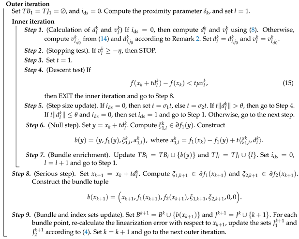
4. The Proposed BEM-DC Algorithm

In this section, we describe the BEM-DC algorithm for solving Problem (1) and give its step-by-step format. The algorithm has both inner and outer iterations. The inner iteration contains the evaluation, in terms of the decrease in the objective function, of tentative displacements from the current point. Null steps might occur within the inner iteration whenever a sufficient decrease is not achieved. Once, instead, such reduction is obtained (serious step), the current estimate of the minimum is updated and a new outer iteration takes place. Based on Proposition 1, a subgradient accumulation process takes place any time a null step occurs within the inner iteration. The specific feature of the BEM-DC algorithm is such that a process involves only information about the function f 1 which is stored in a temporary bundle of tuples, thus exclusively enriching the bundle J 1 k .
Let us denote the outer iteration counter by k. We use l to count for the l-th inner iteration within the k-th outer iteration. Denote the current temporary bundle by T B l and its corresponding index set by T J l . Then, the displacement finding subproblem (5) at the inner iteration l within the k-th iteration takes the following form:
w l k = min d w l k ( d ) .
Define
d l k = arg min d w l k ( d ) = arg min d h l k ( d ) + 1 2 δ k d 2 , and v l k = h l k ( d l k ) .
Then, considering the presence of two distinct bundles for the function f, we have
h l k ( d ) = h 1 , l k ( d ) h 2 k ( d ) ,
where
h 1 , l k ( d ) = max { max j J 1 k ξ 1 , j k , d α 1 , j k , max j T J l ξ 1 , j k , d α 1 , j k } = max j J 1 k T J l ξ 1 , j k , d α 1 , j k , and h 2 k ( d ) = max j J 2 k ξ 2 , j k , d α 2 , j k .
The sets T B l and T J l are updated at each inner iteration, while they are reset to the empty sets at the beginning of each outer iteration. Note that the set J 2 k remains unchanged during the inner iteration process.
Let us focus on Problem (8). Note that it is a DC programming problem whose global optimal solution can be found by solving | J 2 k | convex problems (see [29,33]). Consider the following (convex) problem P l , j k , j J 2 k :
min d w l , j k ( d )
with
w l , j k ( d ) = h 1 , l k ( d ) ξ 2 , j k , d α 2 , j k + 1 2 δ k d 2 .
Let d l , j k = arg min d w l , j k ( d ) . It is clear that, defining
j * = arg min j J 2 k w l , j k ( d l , j k ) ,
the global optimal solution of Problem (8) is
d l k = d l , j * k = arg min d w l , j * k ( d ) , and v l k = h l k ( d l k ) = h 1 , l k ( d l k ) ξ 2 , j * k , d l k α 2 , j * k .
Summing up, d l k is a global optimal solution of Problem (8), and the couple ( d l k , v l k ) is the unique optimal solution of the convex problem P l , j * k
min d R n , v R v + 1 2 δ k d 2 v ξ 1 , j k ξ 2 , j * k , d α 1 , j k α 2 , j * k , j J 1 k T J l .
Then, applying the standard duality arguments to Problem (9), we have the following primal-dual relations:
d l k = 1 δ k j J 1 k T J l λ j ξ 1 , j k ξ 2 , j * k ,
v l k = 1 δ k j J 1 k T J l λ j ξ 1 , j k ξ 2 , j * k 2 j J 1 k T J l λ j α 1 , j k + α 2 , j * k ,
w l k = 1 2 δ k j J 1 k T J l λ j ξ 1 , j k ξ 2 , j * k 2 j J 1 k T J l λ j α 1 , j k + α 2 , j * k .
Here, λ j 0 , j J 1 k T J l , with j J 1 k T J l λ j = 1 , are the optimal variables of the dual of Problem (9). In addition, the definition of the set of problems P l , j k , j J 2 k implies that
w l k = min d w l k ( d ) = w l , j * k ( d l , j * k ) w l , j k ( d l , j k ) , j J 2 k .
Since in the bundle index set J 2 k , there exists an index, say j 0 , associated with the tuple b ( x k ) (see (3)) for which ξ 2 , j 0 k f 2 ( x k ) and α 2 , j 0 k = 0 , we have
w l k w l , j 0 k = w l , j 0 k ( d l , j 0 k ) = 1 2 δ k j J 1 k T J l λ j 0 ξ 1 , j k ξ 2 , j 0 k 2 j J 1 k T J l λ j 0 α 1 , j k ,
for λ j 0 0 , j J 1 k T J l , with j J 1 k T J l λ j 0 = 1 . This together with (12) suggests a possible termination criterion for the proposed algorithm. In fact, whenever w l k η , we have
1 2 δ k j J 1 k T J l λ j 0 ξ 1 , j k ξ 2 , j 0 k 2 + j J 1 k T J l λ j 0 α 1 , j k η ,
which indicates that the subgradient ξ 2 , j 0 k f 2 ( x k ) is at a distance not bigger than 2 δ k η from the ε -subdifferential of f 1 at x k , where
ε = j J 1 k T J l λ j 0 α 1 , j k η .
This property can be interpreted as the approximate satisfaction at the point x k of criticality. Nevertheless, we implement the termination test of the proposed algorithm in the more common form of v l k η . In fact, from (10) and (11), v l k η implies w l k η . Further, the fulfillment of the condition w l , j 0 k η provides an alternative termination criterion as
v l , j 0 k = 1 δ k j J 1 k T J l λ j 0 ξ 1 , j k ξ 2 , j 0 k 2 j J 1 k T J l λ j 0 α 1 , j k η .
Remark 2. 
In the above case, we embed the switching direction technique. That is, we use d l k as a tentative displacement, and if the descent failure occurs, then we implement an Armijo-type line search along the direction d l , j 0 k . Only in the case of failure of the latter is a null step declared.
Next, we present the proposed BEM-DC algorithm 1 in the step-by-step format. We denote by i d s = 1 when the switching direction technique is embedded.
Algorithm 1: BEM-DC
  • Require: The stopping tolerance parameter η > 0 , the null step parameter θ > 0 , the proximity threshold δ m i n > 0 , the sufficient descent parameter μ ( 0 , 1 ) , and the step size reduction parameters σ 1 , σ 2 ( 0 , 1 ) .
  • Ensure: An approximate critical points of Problem (1).
    • Select a starting point x 1 R n . Compute ξ 1 , 1 f 1 ( x 1 ) and ξ 2 , 1 f 2 ( x 1 ) .
    • Set B 1 = { x 1 , f 1 ( x 1 ) , f 2 ( x 1 ) , ξ 1 , 1 , ξ 2 , 1 , 0 , 0 } , J 1 1 = { 1 } , J 2 1 = { 1 } , and k = 1 .
Algorithms 16 00394 i001
Remark 3. 
We update the proximity parameter δ k using the following formula given in [46]:
δ ¯ k + 1 = δ k 1 f ( x k + d k ) f ( x k ) v k , δ k + 1 = max δ ¯ k + 1 , δ k / 10 , δ m i n .
Remark 4. 
An outline of the main differences between BEM-DC and PBDC described in [29] is in order.
  • In BEM-DC, only one of the two subgradients ξ 1 , j and ξ 2 , j , gathered at any iteration j, enters into the calculation of the tentative displacement at each of the successive iterations; the choice is driven by the sign of the linearization error at the current iterate. This is not the case in PBDC;
  • In BEM-DC, there exists a temporary bundle whose “birth and death” takes place within the procedure for escaping from the null step and does not increase the bundle size once a descent is achieved, while PBDC adds more information to the bundles at each step and, thus, increases the bundle sizes at every iteration;
  • In BEM-DC, a second direction is checked for the descent before the null step is declared (see Remark 2), whereas there is only one possible direction used in each step of PBDC.

5. Termination Property of Algorithm BEM-DC

In this section, we provide the proof of the Algorithm BEM-DC, taking any starting point x 1 R n as an input, that returns an approximate critical point x * . Assume that the set
F 1 x R n : f ( x ) f ( x 1 )
is bounded and the numbers L 1 and L 2 are the Lipschitz constants of f 1 and f 2 , respectively, on the set F 1 . Note that, whenever the tuple b ( y ) is inserted into the temporary bundle T B l associated with the function f 1 at the trial point y (see Step 6), then t d l k θ implies ξ 1 + ( y ) ε f 1 ( x k ) for ε 2 θ L 1 θ , where L 1 θ is the Lipschitz constant of f 1 on the set
F θ x R n : d i s t ( x , F 1 ) θ .
Lemma 1. 
Let L 1 θ and L 2 be the Lipschitz constants of f 1 and f 2 , respectively, on the set F θ . Then the following bound holds:
d l k L 1 θ + L 2 δ m i n = D .
Proof. 
Throughout the algorithm, we have δ k δ m i n , and thus, the inequality follows from (10).    □
Remark 5. 
The bound given in (17) is also valid for d l , j 0 * .
Next, we prove that the number of inner iterations of algorithm BEM-DC is finite.
Lemma 2. 
At any given k-th outer iteration, the inner iteration terminates, either fulfilling the sufficient decrease condition (Step 4) or satisfying the stopping condition (Step 2).
Proof. 
Suppose by contradiction that the inner iteration does not terminate. Since (see Remark 5) d l , j 0 * is bounded and t becomes arbitrarily small, the algorithm cannot loop infinitely many times between Steps 4 and 5. Thus, it loops infinitely many times between Steps 1 and 7, giving rise to an infinite number of null steps.
Observe now that every time a null step occurs and the tuple b ( y ) is generated at Step 6, we have
f ( x k + t l d l k ) f ( x k ) = f 1 ( x k + t l d l k ) f 2 ( x k + t l d l k ) f 1 ( x k ) f 2 ( x k ) t l μ v l k , for some 0 < t l < 1 .
Considering
α 1 , l + 1 k = f 1 ( x k ) f 1 ( x k + t l d l k ) + t l ξ 1 , l + 1 k , d l k ,
the convexity of f 2 , and ξ 2 , j 0 k f 2 ( x k ) , it follows
ξ 1 , l + 1 k ξ 2 , j 0 k , d l k α 1 , l + 1 k 1 t l 1 α 1 , l + 1 k + μ v l k > μ v l k .
Furthermore, since the sequence { w l k } l , is monotonically non-decreasing and bounded from above by zero, it is convergent. Note that the sequence { w l , j 0 k } l (see (13)) is convergent as well. Consequently, from boundedness of d l , j 0 k , there exists a convergent subsequence { d l , j 0 k } l L d ¯ 0 k , and thus, the subsequence { v l , j 0 k } l L also converges to a limit, say v ¯ 0 k 0 , for some subset of indices L { 1 , 2 , } .
Next, consider two successive indices p , q L . From (18) and the definition of Problem P l , j 0 k , we obtain
ξ 1 , p + 1 k ξ 2 , j 0 k , d p k α 1 , p + 1 k > μ v p , j 0 k , and ξ 1 , p + 1 k ξ 2 , j 0 k , d q k α 1 , p + 1 k v q , j 0 k .
Therefore, we obtain
v q , j 0 k μ v q , j 0 k > ξ 1 , p + 1 k ξ 2 , j 0 k , d q k d p k .
Passing this to the limit, we have ( 1 μ ) v ¯ 0 k 0 , which, taking into account v ¯ 0 k 0 , implies v ¯ 0 k = 0 . This contradicts that the stopping condition at Step 2 is not satisfied infinitely many times.    □
The next theorem proves the termination of Algorithm BEM-DC.
Theorem 1. 
For any starting point x 1 R n , the algorithm terminates after finitely many iterations at a point satisfying the stopping criterion at Step 2.
Proof. 
Assume the contrary. That is, the stopping criterion at Step 2 is never fulfilled. This implies, taking into account Lemma 2, that an infinite sequence of serious steps takes place, giving rise to infinitely many outer iterations.
Note that every time a serious step is achieved, considering the failed stopping test at Step 2, we have v l k η < 0 . Furthermore, it holds that either t = 1 or t d k > θ . Consequently, it follows from (15) that in the case of t = 1 , we obtain
f ( x k + t d k ) f ( x k ) < μ η ,
or in the second case, considering (17), we have
f ( x k + t d k ) f ( x k ) < μ η θ D .
This together with (19) implies that the decrease of the objective function value in both cases is bounded away from zero every time a serious step occurs. This is a contradiction under the assumption that F 1 is bounded.    □
Remark 6. 
The “escape procedure” (Algorithm 1, introduced in [33]) can escape from critical points which are not Clarke stationary. Algorithm BEM-DC can be combined with this procedure to design an algorithm for finding Clarke stationary points of Problem (1). More precisely, once an approximate critical point is obtained byBEM-DC, the escape procedure could be applied to approximate the Clarke subdifferential at this point [42,43]. Then, it verifies whether this approximation contains the origin with respect to some tolerance. During this approximation, the procedure generates directions that are used to find elements of the Clarke subdifferential. It is proved that this procedure is finitely convergent. That is, after a finite number of steps, it either confirms that the current critical point is also Clarke stationary or the descent direction is found to escape this point (see [33] for more details about different stationary points and their relationships).

6. Numerical Experiments

To evaluate the performance of the BEM-DC algorithm and to compare it with some existing nonsmooth DC programming algorithms, we carry out numerical experiments using different known academic test problems designed for DC programming. Problems 1–9 are from [29], Problems 11–14 are described in [33], and Problems 15–17 are designed in [36]. We exclude Problem 10 from [29] in our experiments as it has many local minimizers and its usage does not provide an unbiased picture of the performance of local search solvers. For the formulations, optimal values, and initial points of these test problems, we refer to references [29,33,36].

6.1. Solvers and Parameters

We consider the following nonsmooth DC optimization solvers in our comparison:
  • Augmented subgradient method for nonsmooth DC optimization (ASM-DC) [36];
  • Aggregate subgradient method for nonsmooth DC optimization (AggSub) [35];
  • Proximal bundle method for nonsmooth DC optimization (PBDC) [29];
  • DC Algorithm (DCA) [8,20];
  • Proximal bundle method for nonsmooth DC programming (PBMDC) [30];
  • Sequential DC programming with cutting-plane models (SDCA-LP) [25].
The parameters in algorithm BEM-DC are chosen as follows: η = 10 7 , δ m i n = 10 5 , θ = 0.5 , μ = 0.2 , σ 1 = 0.2 , and σ 2 = 0.4 . The same set of parameters is used with all the test problems. The initial value of the proximity parameter is computed according to the recommendation given in [46]; that is, δ 1 = ξ 1 , 1 ξ 2 , 1 . We select the parameters of other algorithms considering the recommendations given in their references.
The algorithms BEM-DC, ASM-DC, AggSub, PBDC, and DCA are implemented in Fortran 95 and compiled using the gfortran compiler. For PBMDC and SDCA-LP, we use their MATLAB implementations, available at http://www.oliveira.mat.br/solvers (accessed on 1 August 2023). Since the SDCA-LP algorithm requires the feasible set to be compact, to apply this method to unconstrained problems, we define a large n-dimensional box around the starting point and consider only those points generated by the SDCA-LP that belong to this box.
We set a time limit for all algorithms. For solvers in MATLAB, we consider the limit to be three hours, and for those in Fortran, the limit is half an hour. The source code of algorithm BEM-DC is freely available on GitHub: https://github.com/SnTa2019/Nonsmooth-Optimization (accessed on 1 August 2023) and at http://napsu.karmitsa.fi/bemdc (accessed on 1 August 2023). We carry out our numerical experiments on a computer with Intel(R) Core (TM), i7-9750H, CPU @ 2.60 GHz, 32GB (RAM), under Windows 10, 64Bits. Since the solvers PBMDC and SDCA-LP are implemented in MATLAB, we do not report their CPU time in our comparison.

6.2. Evaluation Measures and Notations

We report the numbers of function and subgradient evaluations and the final value of the objective function found by algorithms. We also provide the computational time (in seconds) required by the algorithms implemented in the same platform (Fortran). The following notations are used:
  • Prob. is the label of the problem;
  • n is the number of variables;
  • N f is the number of function evaluations for the objective function f;
  • N ξ is the number of subgradient evaluations defined as the average of subgradient evaluations for the DC components f 1 and f 2 ;
  • CPU is the computational time in seconds;
  • f A * is the best value of the objective function obtained by algorithm A.
All methods used in this paper are local search methods. In this case, a method is successful if it can find a stationary point of a problem with the given accuracy. For each test problem, a subset of stationary points is known. This subset contains, in particular, stationary points found in methods used in this paper. We say that an algorithm “A” finds a solution with respect to a tolerance β 1 if
0 f A * f o p t | f o p t | + 1 β 1 ,
where f o p t is the value of the objective function at one of the known stationary points. Otherwise, we say that the solver fails. We set β 1 = 10 4 . In addition, we apply performance profiles, introduced in [47], to analyze the results.

6.3. Results

In this subsection, we report and discuss the results of the numerical experiments. We present the results obtained by algorithms for Problems 1–9 from [29] and Problems 11–14 from [33]. We consider two cases by using two types of starting points. In the first case, for each problem, we use one starting point, given in [29,33]. In this case, using tables, we report the values of the objective functions and the numbers of function and subgradient evaluations. In the second case, we use 20 randomly generated starting points for each problem and present the results by applying performance profiles. We also report the average CPU time required by the BEM-DC algorithm on these problems for a different number of variables using both 1 and 20 randomly generated starting points. Further, we show the results for three large-scale test problems from [36] by reporting the values of objective functions and the numbers of function and subgradient evaluations. Table 1, Table 2, Table 3, Table 4 and Table 5 report the results, and the sign “–” is used to show the failure of a method in finding the correct solution.

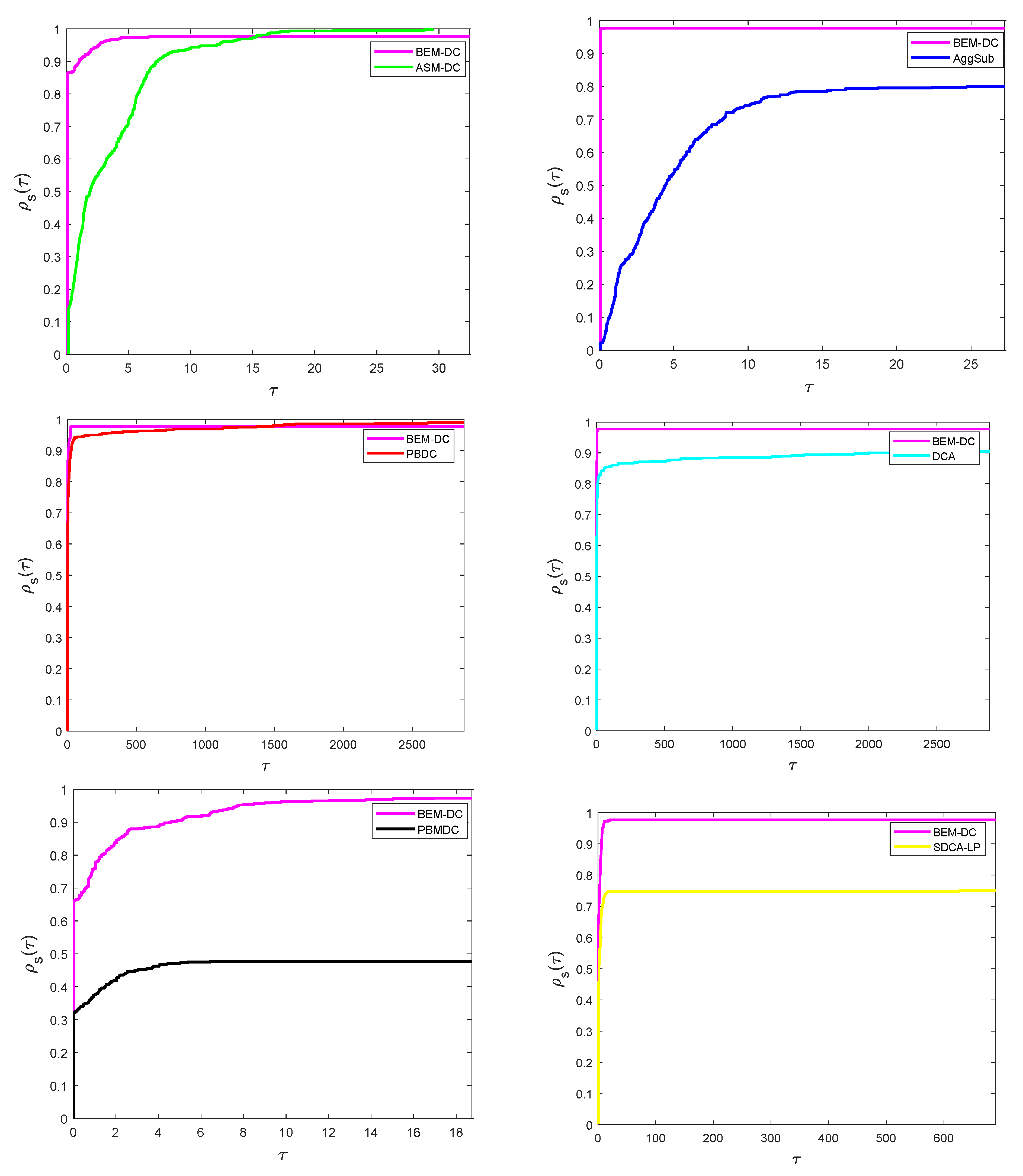
6.3.1. Results with One Starting Point

Table 1 presents the best value of the objective function obtained by solvers using one starting point. We can see that the BEM-DC algorithm is sufficiently accurate in finding local solutions. Except for Problem 9, it finds global minimizers of DC optimization problems in all other cases. Other solvers fail in one or several problems. More specifically, ASM-DC, AggSub, and DCA fail to find solutions in Problem 4 with n = 200 . Furthermore, AggSub fails in Problems 5 and 14 with n = 5 , 10 , 50 , 100 , 200 ; PBDC fails in Problem 12 with n = 50 , 100 , 200 and in Problem 13; DCA fails in Problem 8; PBMDC fails in Problems 7, 12, 13 and also fails in Problem 14 with n = 100 , 200 ; and finally, SDCA-LP fails in Problems 1, 8, 9, 13 and also fails in Problem 12 with n = 10 , 50 , 100 , 200 .
In Table 2, we report the number of function and subgradient evaluations required by the algorithms. These numbers are computed as an average of the number of function and subgradient evaluations of DC components. Note that in SDCA-LP, the number of function and subgradient evaluations are the same. The results show that, in general, PBMDC requires the least number of function and subgradient evaluations among all algorithms. These numbers are similar for PBDC and SDCA-LP. We can see that the computational effort required by the BEM-DC is reasonable and in some instances it is similar to that of by PBMDC, PBDC, and SDCA-LP. Here, Problem 4 with n = 50 , 100 , 200 is an exception. Three other solvers, ASM-DC, AggSub, and DCA also require a reasonable computational effort in most cases; however, in general, they use (in some cases significantly) more function and subgradient evaluations than BEM-DC PBMDC, PBDC, and SDCA-LP.

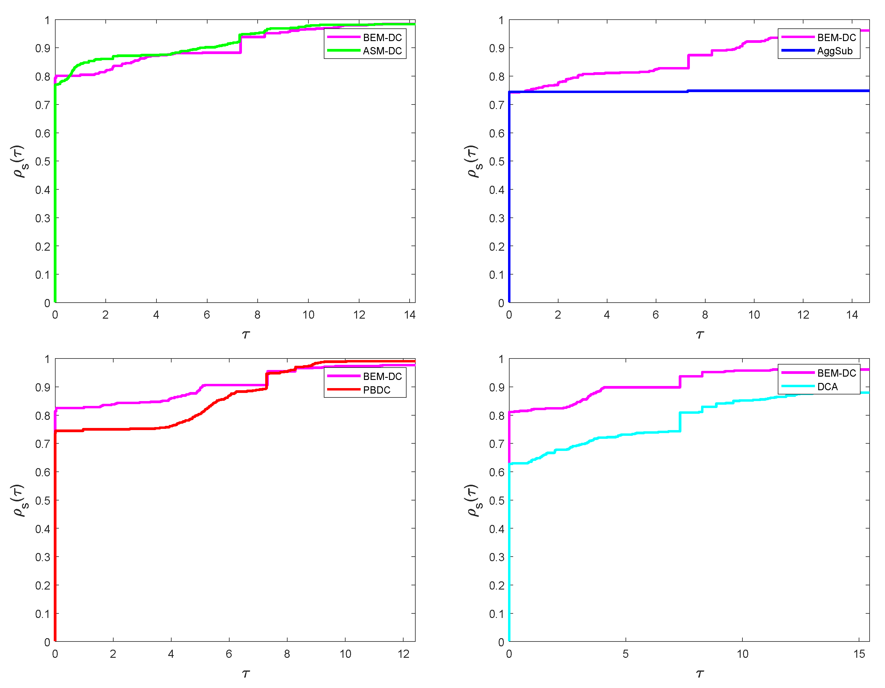
6.3.2. Results with 20 Starting Points

Performance profiles using the number of function evaluations, the number of subgradient evaluations, and the computational time (CPU time) required by algorithms are depicted in Figure 1, Figure 2 and Figure 3. Here, we use results obtained by solving Problems 1–9 and 11–14 with 20 random starting points. We report the pairwise comparison of performance profiles as per the note by [48]. The comparison with other methods shows that the BEM-DC is more efficient and robust than the AggSub, DCA, PBMDC, and SDCA-LP methods. Compared with the ASM-DC method, we can see that the BEM-DC uses significantly fewer subgradient evaluations, and the performance of these two methods are similar concerning two other measures. The performance of the BEM-DC and PBDC methods are similar for the number of function and subgradient evaluations; however, the BEM-DC is more efficient than PBDC if one uses computational time. One reason for this can be the fact that the BEM-DC better manages the bundle of the second DC component than PBDC and decreases the number of the solving of the quadratic programming subproblems required to find search directions.
For a given number n of variables, we also report the average CPU time (in seconds) required by the BEM-DC for Problems 1–9 and 11–14 (29 problems considering different variables) with 1 starting point and 20 random starting points. The results given in Table 3 indicate that the CPU time required by this algorithm is very small for problems with n 10 number of variables.

6.3.3. Results for Large-Scale Problems

Table 4 and Table 5 provide the results obtained by different algorithms for three large-scale problems from [36]: P L 1 , P L 2 , and P L 3 . More specifically, Table 4 contains the best objective function values found by each solver, and Table 5 displays the number of function and subgradient evaluations. As we mentioned above, the number of function and subgradient evaluations are the same for SDCA-LP. Only two algorithms, BEM-DC and ASM-DC, can find approximate solutions to all three problems. AggSub fails in Problem P L 3 , PBDC in Problem P L 1 , DCA in Problems P L 1 and P L 3 , PBMDC in Problem P L 1 , and SDCA-LP in Problems P L 1 and P L 2 . Summarizing results from Table 4, we can conclude that the BEM-DC is the most accurate among all algorithms for solving large-scale problems used in numerical experiments.
Results presented in Table 5 show that among all algorithms, BEM-DC uses the least number of function and subgradient evaluations for solving Problem P L 1 , and PBMDC requires the least computational effort for solving Problems P L 2 and P L 3 . Although the BEM-DC can find accurate solutions for Problems P L 2 and P L 3 , it nevertheless requires more—and in the case of Problem P L 3 , significantly more—function and subgradient evaluations than other solvers. All other algorithms also require reasonable computational effort in problems where they succeeded to find solutions.

7. Conclusions

In this paper, a new method, named the bundle enrichment method (BEM-DC), is introduced for solving nonsmooth unconstrained difference of convex (DC) optimization problems. This method belongs to the family of bundle-type methods. It exploits cutting plane models of DC components to build the model of the DC objective function. The main difference between the proposed method and other bundle methods for DC optimization is in the dynamic management of the bundle. In the implementation of most bundle methods, the size of the bundle for the cutting plane models of the second DC component is given by the user, and it is restricted to reduce the number of subproblems for finding search directions. However, in the BEM-DC, this size is self-determined by the method. This allows for avoiding solving subproblems that do not provide descent directions.
We prove that the BEM-DC computes approximate critical points of the unconstrained DC optimization problems in a finite number of iterations. The performance of this method is evaluated using two groups of nonsmooth DC optimization test problems: small- and medium-sized sized test problems and test problems with a large number of variables. We consider two types of starting points for problems from the first group: the single starting point available in the literature and 20 randomly generated starting points. The use of randomly generated starting points allows us to investigate the robustness of the proposed method. In addition, we provide a comparison of the BEM-DC with six other DC optimization methods.
Results of numerical experiments show that the BEM-DC is able to find accurate solutions using reasonable computational effort in most test problems. Nevertheless, in some large-scale problems, the number of function and subgradient evaluations required by the BEM-DC algorithm may increase significantly as the number of variables increases. This means that the BEM-DC algorithm may not be applicable to some nonsmooth DC optimization problems with a very large number of variables ( n 5000 ). The extension of this method for solving such problems will be the subject of future research.
The remarkable feature of the BEM-DC is that it is able to dynamically manage the number of subgradients of the second DC components and significantly decrease the number of quadratic programming subproblems for finding search directions. Results obtained using many randomly generated starting points allow us to conclude that the BEM-DC is efficient and is among the most robust methods used in numerical experiments. Further, the BEM-DC algorithm is able to efficiently solve relatively large nonsmooth DC optimization problems.

Author Contributions

All authors contribute equally. All authors have read and agreed to the published version of the manuscript.

Funding

A.M. Bagirov’s research is funded by the Australian Government through the Australian Research Council’s Discovery Projects (Project No. DP190100580), and the research by N. Karmitsa is supported by the Research Council of Finland (Projects No. 345804 and No. 345805).

Data Availability Statement

The source code of BEM-DC is freely available on GitHub: https://github.com/SnTa2019/Nonsmooth-Optimization (accessed on 1 August 2023) and at http://napsu.karmitsa.fi/bemdc (accessed on 1 August 2023).

Acknowledgments

A.M. Bagirov’s research is funded by the Australian Government through the Australian Research Council’s Discovery Projects (Project No. DP190100580), and the research by N. Karmitsa is supported by the Academy of Finland (Projects No. 345804 and No. 345805).

Conflicts of Interest

The authors declare no conflict of interest.

References

  1. Bertsekas, D.P. Nonlinear programming. In Theoretical Solutions Manual, 3rd ed.; Athena Scientific: Nashua, NH, USA, 2016. [Google Scholar]
  2. Hiriart-Urruty, J.B. Generalized differentiability/ duality and optimization for problems dealing with differences of convex functions. In Lecture Notes in Economics and Mathematical Systems; Springer: Berlin/Heidelberg, Germany, 1986; Volume 256, pp. 37–70. [Google Scholar]
  3. Strekalovsky, A.S. Global optimality conditions for nonconvex optimization. J. Glob. Optim. 1998, 12, 415–434. [Google Scholar] [CrossRef]
  4. Strekalovsky, A.S. On a Global Search in D.C. Optimization Problems. In Optimization and Applications; Springer: Cham, Swizerland, 2020; pp. 222–236. [Google Scholar]
  5. Strekalovsky, A.S. Local Search for Nonsmooth DC Optimization with DC Equality and Inequality Constraints. In Numerical Nonsmooth Optimization; Springer: Cham, Swizerland, 2020; pp. 229–261. [Google Scholar]
  6. de Oliveira, W. The ABC of DC programming. Set-Valued Var. Anal. 2020, 28, 679–706. [Google Scholar] [CrossRef]
  7. Horst, R.; Thoai, N.V. DC programming: Overview. J. Optim. Theory Appl. 1999, 103, 1–43. [Google Scholar] [CrossRef]
  8. An, L.T.H.; Tao, P.D. The DC (difference of convex functions) programming and DCA revisited with DC models of real world nonconvex optimization problems. Ann. Oper. Res. 2005, 133, 23–46. [Google Scholar] [CrossRef]
  9. Holmberg, K.; Tuy, H. A production-transportation problem with stochastic demand and concave production costs. Math. Program. 1999, 85, 157–179. [Google Scholar] [CrossRef]
  10. Pey-Chun, C.; Hansen, P.; Jaumard, B.; Tuy, H. Solution of the multisource Weber and conditional Weber problems by DC programming. Oper. Res. 1998, 46, 548–562. [Google Scholar] [CrossRef]
  11. Khalaf, W.; Astorino, A.; D’Alessandro, P.; Gaudioso, M. A DC optimization-based clustering technique for edge detection. Optim. Lett. 2017, 11, 627–640. [Google Scholar] [CrossRef]
  12. Sun, X.K. Regularity conditions characterizing Fenchel–Lagrange duality and Farkas-type results in DC infinite programming. J. Math. Anal. Appl. 2014, 414, 590–611. [Google Scholar] [CrossRef]
  13. Bagirov, A.M.; Karmitsa, N.; Taheri, S. Partitional Clustering via Nonsmooth Optimization; Springer: Berlin/Heidelberg, Germany, 2020. [Google Scholar]
  14. Bagirov, A.M.; Taheri, S.; Cimen, E. Incremental DC Optimization Algorithm for Large-Scale Clusterwise Linear Regression. J. Comput. Appl. Math. 2021, 389, 113323. [Google Scholar] [CrossRef]
  15. Sun, X.; Teo, K.L.; Zeng, J.; Liu, L. Robust approximate optimal solutions for nonlinear semi-infinite programming with uncertainty. Optimization 2020, 69, 2109–2129. [Google Scholar] [CrossRef]
  16. Sun, X.; Tan, W.; and Teo, K.L. Characterizing a Class of Robust Vector Polynomial Optimization via Sum of Squares Conditions. J. Optim. Theory Appl. 2023, 197, 737–764. [Google Scholar] [CrossRef]
  17. Sun, X.; Teo, K.L.; Long, X.J. Some characterizations of approximate solutions for robust semi-infinite optimization problems. J. Optim. Theory Appl. 2021, 191, 281–310. [Google Scholar] [CrossRef]
  18. Tuy, H. Convex Analysis and Global Optimization; Kluwer: Dordrecht, The Netherlands, 1998. [Google Scholar]
  19. Tao, P.D.; Souad, E.B. Algorithms for solving a class of nonconvex optimization problems: Methods of subgradient. North-Holl. Math. Stud. 1986, 129, 249–271. [Google Scholar]
  20. An, L.T.H.; Tao, P.D.; Ngai, H.V. Exact penalty and error bounds in DC programming. J. Glob. Optim. 2012, 52, 509–535. [Google Scholar]
  21. Artacho, F.J.A.; Fleming, R.M.T.; Vuong, P.T. Accelerating the DC algorithm for smooth functions. Math. Program. 2018, 169, 95–118. [Google Scholar] [CrossRef]
  22. Artacho, F.J.A.; Vuong, P.T. The Boosted Difference of Convex Functions Algorithm for Nonsmooth Functions. Siam J. Optim. 2020, 30, 980–1006. [Google Scholar] [CrossRef]
  23. de Oliveira, W.; Tcheou, M.P. An inertial algorithm for DC programming. Set-Valued Var. Anal. 2019, 27, 895–919. [Google Scholar] [CrossRef]
  24. Artacho, F.J.A.; Campoy, R.; Vuong, P.T. Using positive spanning sets to achieve d-stationarity with the boosted DC algorithm. Vietnam. J. Math. 2020, 48, 363–376. [Google Scholar] [CrossRef]
  25. de Oliveira, W. Sequential difference-of-convex programming. J. Optim. Theory Appl. 2020, 186, 936–959. [Google Scholar] [CrossRef]
  26. Dolgopolik, M.V. A convergence analysis of the method of codifferential descent. Comput. Optim. Appl. 2018, 71, 879–913. [Google Scholar] [CrossRef]
  27. Gaudioso, M.; Giallombardo, G.; Miglionico, G. Minimizing piecewise-concave functions over polytopes. Math. Oper. Res. 2018, 43, 580–597. [Google Scholar] [CrossRef]
  28. Gaudioso, M.; Giallombardo, G.; Miglionico, G.; Bagirov, A.M. Minimizing nonsmooth DC functions via successive DC piecewise-affine approximations. J. Glob. Optim. 2018, 71, 37–55. [Google Scholar] [CrossRef]
  29. Joki, K.; Bagirov, A.M.; Karmitsa, N.; Mäkelä, M.M. A proximal bundle method for nonsmooth DC optimization utilizing nonconvex cutting planes. J. Glob. Optim. 2017, 68, 501–535. [Google Scholar] [CrossRef]
  30. de Oliveira, W. Proximal bundle methods for nonsmooth DC programming. J. Glob. Optim. 2019, 75, 523–563. [Google Scholar] [CrossRef]
  31. Sun, W.Y.; Sampaio, R.J.B.; Candido, M.A.B. Proximal point algorithm for minimization of DC functions. J. Comput. Math. 2003, 21, 451–462. [Google Scholar]
  32. Souza, J.C.O.; Oliveira, P.R.; Soubeyran, A. Global convergence of a proximal linearized algorithm for difference of convex functions. Optim. Lett. 2016, 10, 1529–1539. [Google Scholar] [CrossRef]
  33. Joki, K.; Bagirov, A.M.; Karmitsa, N.; Mäkelä, M.M.; Taheri, S. Double bundle method for finding Clarke stationary points in nonsmooth DC programming. Siam J. Optim. 2018, 28, 1892–1919. [Google Scholar] [CrossRef]
  34. Ackooij, W.; Demassey, S.; Javal, P.; Morais, H.; de Oliveira, W.; Swaminathan, B. A bundle method for nonsmooth dc programming with application to chance–constrained problems. Comput. Optim. Appl. 2021, 78, 451–490. [Google Scholar] [CrossRef]
  35. Bagirov, A.M.; Taheri, S.; Joki, K.; Karmitsa, N.; Mäkelä, M.M. Aggregate subgradient method for nonsmooth DC optimization. Optim. Lett. 2020, 15, 83–96. [Google Scholar] [CrossRef]
  36. Bagirov, A.M.; Hoseini, M.N.; Taheri, S. An augmented subgradient method for minimizing nonsmooth DC functions. Comput. Optim. Appl. 2021, 80, 411–438. [Google Scholar] [CrossRef]
  37. Astorino, A.; Frangioni, A.; Gaudioso, M.; Gorgone, E. Piecewise quadratic approximations in convex numerical optimization. SIAM J. Optim. 2011, 21, 1418–1438. [Google Scholar] [CrossRef]
  38. Bagirov, A.M.; Gaudioso, M.; Karmitsa, N.; Mäkelä, M.M.; Taheri, S. (Eds.) Numerical Nonsmooth Optimization, State of the Art Algorithms; Springer: Berlin/Heidelberg, Germany, 2020. [Google Scholar]
  39. Gaudioso, M.; Monaco, M.F. Variants to the cutting plane approach for convex nondifferentiable optimization. Optimization 1992, 25, 65–75. [Google Scholar] [CrossRef]
  40. Hiriart–Urruty, J.B.; Lemaréchal, C. Convex Analysis and Minimization Algorithms; Springer: Berlin, Germany, 1993; Volume I and II. [Google Scholar]
  41. Bagirov, A.M.; Karmitsa, N.; Mäkelä, M.M. Introduction to Nonsmooth Optimization: Theory, Practice and Software; Springer: New York, NY, USA, 2014. [Google Scholar]
  42. Mäkelä, M.M.; Neittaanmäki, P. Nonsmooth Optimization; World Scientific: Singapore, 1992. [Google Scholar]
  43. Clarke, F.H. Optimization and Nonsmooth Analysis; John Wiley & Sons: New York, NY, USA, 1983. [Google Scholar]
  44. Demyanov, V.F.; Vasilev, L.V. Nondifferentiable Optimization; Springer: New York, NY, USA, 1985. [Google Scholar]
  45. Polyak, B.T. Minimization of unsmooth functionals. Ussr Comput. Math. Math. Phys. 1969, 9, 14–29. [Google Scholar] [CrossRef]
  46. Kiwiel, K.C. Proximity control in bundle methods for convex nondifferentiable minimization. Math. Program. 1990, 46, 105–122. [Google Scholar] [CrossRef]
  47. Dolan, E.D.; More, J.J. Benchmarking optimization software with performance profiles. Math. Program. 2002, 91, 201–213. [Google Scholar] [CrossRef]
  48. Gould, N.; Scott, J. A note of performance profiles for benchmarking software. Acm Trans. Math. Softw. 2016, 43, 1–5. [Google Scholar] [CrossRef]
Figure 1. Performance profiles using the number of function evaluations (20 starting points).
Algorithms 16 00394 g001
Figure 2. Performance profiles using the number of subgradient evaluations (20 starting points).
Algorithms 16 00394 g002
Figure 3. Performance profiles using CPU time (20 starting points).
Algorithms 16 00394 g003
Table 1. Best values of the objective functions obtained by solvers (one starting point).
Prob.nBEM-DCASM-DCAggSubPBDCDCAPBMDCSDCA-LP
122.000002.000002.000002.000002.000002.00000
220.000000.000000.000000.000001.000000.000000.00000
340.000000.000010.000010.000000.000000.000002.00000
420.000000.000000.000000.000000.000000.000000.00000
450.000000.000000.000000.000000.000000.000000.00000
4100.000000.000000.000000.000000.000000.000000.00000
4500.000000.000000.000000.000000.000000.000000.00000
41000.000000.000000.000000.000000.000000.000000.00000
42000.000000.000000.000000.00000
520.000000.000000.000000.000000.000000.000000.00000
550.000000.000000.000000.000000.000000.00000
5100.000010.000000.000000.000000.000000.00001
5500.000040.000010.000000.000110.000000.00002
51000.000000.000010.000000.000310.000000.00007
52000.000000.000010.000000.000030.000000.00008
62−2.50000−2.50000−2.50000−2.50000−2.50000−2.50000−2.50000
720.500000.500000.500000.500001.000000.50000
833.500003.500003.500003.500003.50000
949.200009.200009.200001.833339.200001.83333
113116.33333116.33333116.33377116.33333116.33333116.33330116.33330
1220.618040.618040.618041.618030.618031.61809
1250.618030.618040.618041.618030.618030.61803
12100.618030.618040.618040.618030.61803
12500.618030.618040.618040.61804
121000.618030.618030.618040.61804
122000.618030.618030.618040.61804
13100.000000.000000.000000.00000
1420.000000.000000.000000.000000.000000.000000.00000
1450.000010.000000.000000.000000.000010.00001
14100.000000.000000.000000.000000.000010.00003
14500.000020.000000.000000.000000.000020.00005
141000.000070.000010.000000.000000.00006
142000.000030.000030.000000.000000.00003
Table 2. Number of function and subgradient evaluations required by solvers (one starting point).
Prob.nBEM-DCASM-DCAggSubPBDCDCAPBMDCSDCA-LP
N f N ξ N f N ξ N f N ξ N f N ξ N f N ξ N f N ξ N f , N ξ
12105251895216275221760411016
2217525109412559218137254357
3487171495339117423112221815816
42751743196431635228226
45409126442351201361651243413
41070182568854527316103613095826
450186587434301124320615975232291528072538103
41009049437910,87835396824340510266631262325075204
420040,71319,626475546101151403
52832315075311843724238
55642611844157474297689
5108742335111231554,11653,287122434
5505262351413457135124247,813246,256172455
51001417113374384725471,198469,845202963
52001296518855941085246,2821461,267182866
623910135431055522144133172429
723034838811128510772473368247149
831254927175176886032
94931996316980867263561725
113146281746125812610718175814
1221302629079127642015616037
1252025245712221310358396765696
1210393105831257359170141512577674
1250739156301577114116949997
121001032173699825191239907117115
12200275717415,302509028501397338337
131014521261370382019
14219450237134955654111629
14514526206732261001091056361223158
1410249593571073221556169615161603450107
14501168439672211165379099196616145989280
14100227370817795497807401816552
14200259172417465419839612826619
Table 3. CPU time (in seconds) required by BEM-DC.
n23451050100
1 starting point0.0000.0000.0010.0120.0090.67216.328
20 starting points0.0000.0000.0020.0180.61614.61342.461
Table 4. Best values of objective functions obtained by solvers for large-scale problems.
PnBEM-DCASM-DCAggSubPBDCDCAPBMDCSDCA-LP
P L 1 2000.000000.000060.0000798.56721153.29050
P L 1 5000.000000.000090.00007249.00000539.99295
P L 1 10000.000000.000320.00032499.00000510.84581
P L 1 15000.000000.000720.00051749.00000 1.90755 × 10 3
P L 1 20000.000000.002470.00083999.00000 1.00229 × 10 3
P L 2 2000.000000.000000.000000.000000.000000.00000 3.59539 × 10 3
P L 2 5000.000000.000000.000000.000000.000000.00000 1.08151 × 10 4
P L 2 10000.000000.000000.000000.000000.000000.00001 2.43987 × 10 4
P L 2 15000.000000.000000.000000.000000.000000.00002 3.90289 × 10 4
P L 2 20000.000000.000000.000000.000000.000000.00003 5.43386 × 10 4
P L 3 2000.000040.000004.665260.000000.161240.000010.00005
P L 3 5000.000010.000017.912750.000000.083520.000020.00015
P L 3 10000.000060.0003717.321600.000000.050600.000010.00004
P L 3 15000.000020.0015710.501610.000002.787350.000010.00011
P L 3 20000.000080.0005612.630330.0000026.174930.000020.00003
Table 5. Number of function and subgradient evaluations for large-scale problems.
Prob.nBEM-DCASM-DCAggSubPBDCDCAPBMDCSDCA-LP
N f N ξ N f N ξ N f N ξ N f N ξ N f N ξ N f N ξ N f , N ξ
P L 1 20049323286281075277604825082502
P L 1 5009432083456140036414611520062002
P L 1 1000158321654972127607503735113503
P L 1 15002184269166417344791028010031001
P L 1 2000244431237931299631493445264515
P L 2 20086324818355931604787974780501050051081774509
P L 2 50014304242161705234211571355105750105005144232264
P L 2 100035891057315310412277112516641416590458962193601655
P L 2 150042931329396613102722134420441740415841532954821509
P L 2 20006433181744331466293614592244191455115505299497955
P L 3 200198953610443331463971511928184530063003559797
P L 3 50045987291444469128696252253925133507350358993555
P L 3 100013,84430063445110721,45610,555298029583006300373126370
P L 3 150012,3842291240873041,09620,2392763274715031501691211130
P L 3 200017,52031564017128334,75817,1493766374115031501731271090
Disclaimer/Publisher’s Note: The statements, opinions and data contained in all publications are solely those of the individual author(s) and contributor(s) and not of MDPI and/or the editor(s). MDPI and/or the editor(s) disclaim responsibility for any injury to people or property resulting from any ideas, methods, instructions or products referred to in the content.

