Abstract
This paper presents a novel approach utilizing uniform rectangular arrays to design a constant-beamwidth (CB) linearly constrained minimum variance (LCMV) beamformer, which also improves white noise gain and directivity. By employing a generalization of the convolutional Kronecker product beamforming technique, we decompose a physical array into virtual subarrays, each tailored to achieve a specific desired feature, and we subsequently synthesize the original array’s beamformer. Through simulations, we demonstrate that the proposed approach successfully achieves the desired beamforming characteristics while maintaining favorable levels of white noise gain and directivity. A comparative analysis against existing methods from the literature reveals that the proposed method performs better than the existing methods.
1. Introduction
Beamformers play a crucial role in diverse fields, such as telecommunications [1], acoustics [2,3], hearing aids [4], and others [5,6,7,8]. Among the array configurations used for beamforming, rectangular arrays are an interesting option to be explored [9,10,11], as they offer distinct advantages over linear arrays, providing enhanced spatial information regarding impinging sources [12,13] and reduced redundancy due to their asymmetry [14].
The development of robust adaptive beamformers with frequency-invariant characteristics has been a significant point of interest as, in this case, frequency does not affect the behavior of the beamformer. Some desired features are a constant beamwidth [15] and null steering [16]. One approach for null steering is using a linearly constrained minimum variance (LCMV) beamformer [17,18,19], which cancels interfering signals from given directions and steers the main beam toward the desired signal. However, it lacks a robust mechanism for maintaining a constant beamwidth. Constant-beamwidth (CB) beamforming [15,20,21] can be accomplished by using window-based beamforming techniques [22], but these methods cannot incorporate directional restrictions. CB-LCMV beamformers have been recently explored [23], however only in the context of linear sensor arrays, leaving space for their study in the context of different array configurations.
Other metrics that are desired to be enhanced are white noise gain and directivity factor, which can respectively be maximized by the delay-and-sum (DS) and superdirective (SD) beamformers [24]. Another quality that is often required for designing a beamformer is a distortionless response to the desired source or to the desired source direction. This ensures that the desired signal is unaltered by filtering processes.
While constructing a beamformer with multiple beamforming features is non-trivial, efforts have been made to combine multiple beamforming techniques for a single array of sensors. Two notable approaches are the Kronecker product (KP) method [25,26] and the linear convolutional Kronecker product (LCKP) method [23]. The LCKP method is valid only for linear arrays, however it allows for the virtual utilization of more sensors than are physically available [23]. Meanwhile, the KP method can be used in linear or rectangular arrays, but it does not increase the number of sensors available for beamforming. For both combination methods (the KP and LCKP), beampattern features and distortionless constraints are preserved in the combined beamformers. Therefore, by using beamformers with desired beampattern characteristics that respect the distortionless constraint, these are maintained in the end result.
In this paper, we propose a novel approach to constructing a CB-LCMV beamformer for rectangular arrays. To this end, we generalize the LCKP beamforming technique to the case of rectangular arrays. We synthesize beamformers for virtual subarrays and, with our proposed generalized technique, apply them to a full array to achieve the desired beamwidth and null placement. This is achieved without sacrificing white noise gain or the directivity factor. The performance of the proposed method is compared against that of beamformers obtained through the KP and LCKP methods. Our results demonstrate superior performance in terms of the beamwidth, white noise gain, and directivity of the beamformers obtained using the proposed method when compared to the performance of the beamformers obtained using the methods in the literature.
This paper is organized as follows: Section 2 presents the array and signal model considered for the problem; Section 3 shows the traditional beamforming techniques and methods that are used further. In Section 4, the newly proposed method for an array analysis for rectangular arrays is introduced and detailed, as well as its proposed usage for solving the problem at hand. In Section 5, we present the conducted simulations and discuss the results, comparing them to those in the literature. Finally, Section 6 concludes this paper, presenting an overview of the main contributions.
2. Signal and Array Model
Let S be a uniform rectangular array (URA) of sensors over the plane in an anechoic environment with desired and undesired sources. The URA comprises sensors spaced apart along the -axis and sensors spaced apart along the -axis, resulting in a total of sensors. Assume a source in the far field on the same plane as the sensor array (that is, with elevation ), impinging on it from an azimuth angle . As it is unusual, in speech enhancement, for the desired and undesired sources to have the same azimuth, differing only by elevation, we assume the elevation to be . This constraint can be easily removed without affecting the developed mathematical framework.
Let denote the steering matrix of size with elements given by
where m/s is the speed of sound, are the polar coordinates of the sensor at , is the angular frequency, f is the temporal frequency, and is the imaginary unit. We let denote the steering vector, with and being the vectorization operation, and we let denote the inverse vectorization of .
The observed signal vector for all sensors in the frequency domain can be written as
where is the desired signal at the reference sensor, is the steering vector of the desired source from direction , and is the additive noise signal vector. All signals are assumed to be zero-mean and uncorrelated. We can estimate the desired signal as using the beamformer (assumed to be a 2-D beamformer) through linear filtering,
where the superscript denotes the conjugate-transpose operator. In that case,
where is the residual noise at the beamformer’s output. The beamformer is called distortionless if it satisfies for all . This constraint guarantees that the beamformer does not affect the desired signal, only altering the undesired noise signal.
From here on, is omitted unless in definitions, and in the steering vectors appears in subscripts where necessary. When no angle is shown, is assumed to be the desired signal steering vector for conciseness.
Beamformer Metrics
Beampattern , as a function of beamformer and direction (through steering vector ) is given by
Given the desired signal steering vector , the white noise gain (WNG), desired signal distortion index (DSDI), and directivity factor (DF) are, respectively,
where is the spherical isotropic noise field coherence matrix [27]. Using the DSDI, the distortionless constraint can also be written as .
3. Conventional Beamformers
This section briefly overviews the beamforming techniques used to construct the proposed beamformer, as well as the different methods for beamformer synthesis.
3.1. LCMV Beamformer
Assuming the presence of undesired sources in known directions, a linearly constrained minimum variance (LCMV) beamformer [17,18,19] is useful to position the nulls of the beampattern in those undesired directions. To this end, we assume the existence of N (with ) uncorrelated interfering sources in the far field, each coming from a (different) direction () that we want to cancel. We write as
where is the noise signal for the n-th undesired direction, and is the portion of the noise signal not coming from the N undesired directions, also accounting for acoustic uncorrelated noise. We assume that . We then use linear constraints, representing the distortionless constraint for the desired signal plus the canceling of the N undesired directions.
The LCMV constraint is written in matrix form as
where is an matrix, is an vector, and the superscript denotes the transpose operator. The LCMV beamformer is obtained by minimizing the variance of residual noise in the beamformer output (from Equation (4)), given the constraints in (8), which translates to a minimization problem given as
where is the correlation matrix of , assumed to be a full-rank invertible matrix. As the undesired directions will be canceled (assuming an anechoic environment [28]), this minimization process minimizes , the noise portion that is uncorrelated with the N undesired directions. The solution to this minimization problem is
To ensure the existence of a solution, the number of sensors should be larger than or equal to the number of constraints, i.e., . For , only the distortionless constraint remains, and the LCMV beamformer reduces to a minimum variance distortionless response (MVDR) beamformer [29], which is given by
It is possible to show that the LCMV and MVDR beamformers are also defined in terms of the observed signal correlation matrix [24], in which case
This formulation depends only on the statistics of the observed signal, which are easier to compute than those of the noise signal.
3.2. CB Beamformer
Constant-beamwidth (CB) beamformers guarantee a certain beamwidth around the desired direction that is constant over frequency. This is important to ensure the correct receiving of the desired signal, even if is not precisely calibrated.
We define as the first-null beamwidth (FNBW), such that if . That is, is the first angle in which a null of the beampattern occurs. A constant-beamwidth beamformer can be achieved using a window-based design technique [22]. Here, the Kaiser window is used [30], which can be written as
where is the zero-order modified Bessel function of the first kind, and ([22], Section 3.3.2) is frequency-dependent to maintain the constant. This technique requires that the desired source signal impinges on the array from the broadside direction [22]. To satisfy the distortionless constraint, we normalize , obtaining
3.3. SD and DS Beamformers
Superdirective (SD) and delay-and-sum (DS) beamformers are obtained by maximizing the DF and the WNG, respectively [29,31], both subject to the distortionless constraint. The solutions to these minimization problems are respectively given by
3.4. Kronecker Product Beamforming
Designing a single beamformer with different features is highly important, allowing different effects to be employed over a single array of sensors. Two methods to accomplish such a task are the Kronecker product (KP) [25,26] and linear convolutional Kronecker product (LCKP) methods [23]. In these processes, the sensor array is split into subarrays for which we design separate beamformers and use the chosen technique to synthesize the whole sensor array’s (or full array’s) beamformer.
The KP beamforming process is as follows: given steering vector , we decompose it into two parts (namely, and ) satisfying the relation , where ⊗ represents the Kronecker product. By designing beamformers and for and , respectively, we obtain the beamformer for the full array as [32].
LCKP beamforming is achieved similarly: given a uniform linear array’s (ULA) steering vector of length M, we define as the -th first elements of and, similarly, with elements, respecting . By designing beamformers and for each subarray, the full array’s beamformer is [23], where ∗ denotes the linear convolution.
For both the KP and LCKP methods, we have the following properties:
The first one shows that the beampattern of is the combination of the beampatterns of the subarrays. Through the second one, we can see that, if and are distortionless beamformers, also will be. From these properties, we can see that the beampattern properties (including the distortionless feature) from and are maintained for .
4. Constant-Beamwidth LCMV Beamformer with Rectangular Arrays
Both the KP and LCKP beamforming methods have advantages and disadvantages. While the LCKP is only usable over linear arrays, beamformers achieved through it have (virtually) more sensors than there are available in the physical array, generally leading to better performance when combining different techniques. Meanwhile, the KP method can be applied to rectangular arrays, which on its own is beneficial, but it does not have the virtual utilization of more sensors. To benefit from the lack of symmetry of the rectangular arrays and to also be able to have more sensors available for each subarray’s beamformer, we propose a generalization of the LCKP to URAs to take advantage of both methods, enabling virtual sensor augmentation while exploiting the rectangular array’s symmetry.
4.1. Rectangular Convolutional Kronecker Product Beamforming
Let be a subarray of S, including the first sensors of S, with steering vector , and similarly for . These arrays sizes are such that , and . By designing beamformers and for and , respectively, we show in Appendix A that it is possible to synthesize a beamformer for full array S through
with ⊛ representing the 2-D convolution operation. We call this the rectangular convolutional Kronecker product (RCKP) method. A simple implementation of the proposed RCKP method is presented in Algorithm A1 in Appendix B, which is written in a Python-like pseudolanguage.
In the same way as with the KP and LCKP methods, with the RCKP, one can design beamformers for subarrays and , and one can synthesize the URA’s beamformer through the 2-D convolution (and vectorization processes). Accordingly, is an vector; however, in this scenario we have a total of virtual sensors. Assuming that all Ms are ≥1, it is trivial to see that (equality happens if and are perpendicular ULAs, or if one of them has only one sensor). Therefore, we have more sensors virtually than if S was split into two VAs through the KP method.
It is easy to verify that the properties in (16) are also valid for the proposed RCKP. With this, like for the KP and LCKP, the full-array beamformer obtained through the RCKP inherits the beampattern and distortionless features from the subarray beamformers. Also, since convolution is commutative and associative, one can split the S array into more than two virtual arrays, design a beamformer for each subarray, and combine all the beamformers through the RCKP without the loss of generalization. In this case, assuming that we are using K beamformers, each with size , then their dimensions must be such that
This is easily verifiable by repeating the synthesis operation in Equation (17) times.
4.2. CB-LCMV Beamformer with RCKP
Here, we propose the use of the RCKP method as derived previously to construct a CB-LCMV beamformer with an increase in white noise gain and directivity measures. For this, full array S is separated into four subarrays: , , , and . Each subarray is used to design one of the desired beamformers presented in Section 3.1, Section 3.2 and Section 3.3.
is used to design the LCMV beamformer, following the steps detailed in Section 3.1. Since the LCMV beamformer does not require the array to be linear, we use as a rectangular array of size . As explained previously, this choice has the advantage of the rectangular array’s lesser symmetry compared to a linear array. We have virtual sensors and, at most, nulls to be placed. If , this same array is used for the MVDR beamformer instead.
The subarray is used to construct the CB beamformer. Given that the CB is achieved through the window technique (as per Section 3.2), this subarray must be a ULA, and the desired source direction should be on its broadside direction. Here, this implies that .
The SD and DS beamformers are built from the and subarrays, respectively, based on Section 3.3. We assume that they are constructed from linear arrays, but this condition is flexible and can be changed in other implementations.
Once all the subarray beamformers are designed, we use the RCKP method to combine these beamformers into a full-array beamformer. Thus, we construct a beamformer with many desired features (null placement + constant beamwidth + white noise gain + directivity factor gain) that exploit the symmetry of the rectangular array, which implies more spatial information and more performance. Algebraically, the full-array beamformer is given by
An implementation of the proposed CB-LCMV beamformer is shown in Algorithm A2 in Appendix B. The procedure calculates beamformer for a single frequency.
For the CB beamformer to be effective, its condition must be valid for all beamformers. That is, if , where . This is true by definition for the CB beamformer, and by setting for the LCMV, no nulls are free to end up inside the main beam. For the SD and DS beamformers, we assume that their FNBWs are sufficient to satisfy the condition.
5. Experimental Results
In this section, we present the simulations performed to verify the proposed method’s implementation and to compare its performance to that of existing methods. The code used for these simulations is available at https://github.com/VCurtarelli/py-cb-lcmv-rect (accessed on 27 July 2023). We test different combinations of the number of sensors for each subarray, as established in Table 1. The table presents the dimensions for each subarray, for the full array of sensors, and the virtual number of sensors being employed. [A, B] are obtained through the RCKP, [C, D] through the LCKP, and [E, F] through the KP + LCKP, with the KP and LCKP methods being as defined in Section 3.4. [A, C, E] utilize the SD and DS beamformers, while [B, D, F] “disable” them in favor of the CB beamformer. For [E, F], the LCMV beamformer is more spaced out.

Table 1.
Number of sensors for each subarray, dimension of the full array (FA), and size of the virtual array in each simulation.
In all situations, S has a total of sensors. The sensors are assumed to be ideal omnidirectional sensors with a plain frequency response over the spectrum. The intersensor distances are and . We assume that and . Since the LCMV has four sensors, we use three interfering sources (for all situations), with directions , each with , and we also assume to be uncorrelated Gaussian white noise with unit variance (that is, is the identity matrix). The variance of the desired signal is . The simulations are performed for the range . This range is chosen to satisfy the conditions from ([22], Equation (29)) for condition [A].
Figure 1 and Figure 2a–c show the simulation results for , measured , , and . was measured as the first angle in which . All methods manage to achieve the nulls in the desired directions from the LCMV. Observing Figure 2a, all but [E] are capable of maintaining a reasonable beamwidth across all frequencies, with [E] not being able to maintain the beamwidth because of too few sensors in the CB beamformer. The “naïve” combination of KP and LCKP [E, F] leads to worse performance for all metrics; thus, their results are not further compared.
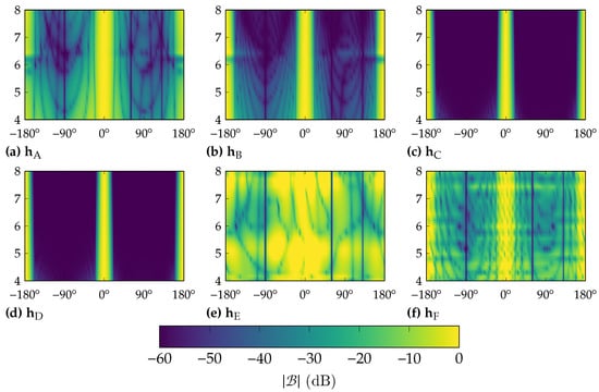
Figure 1.
Beampattern heatmap for all situations in Table 1. -axis is direction of source (in ), and -axis is the frequency (in kHz).
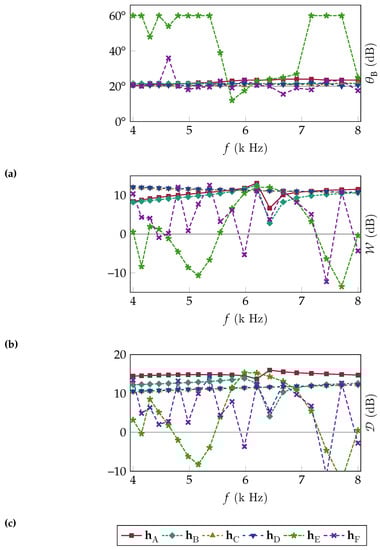
Figure 2.
(a) FNBW, (b) WNG, and (c) DF for the beamformers designed with the parameters in Table 1.
Both methods (the RCKP and LCKP) lead to very akin results for , even though the LCKP simulations [C, D] have many more sensors in the CB beamformer than the RCKP ones [A, B]. This indicates that increasing the CB array size does not result in a better performance in either FNBW or directivity. However, in Figure 1, it can be seen that it generates a more focused beam. Both the RCKP and LCKP have similar WNG results of around 10 dB. The proposed method (especially [A]) leads to a better performance in terms of DF for all frequencies compared to the LCKP. The LCKP is marginally better for WNG in lower frequencies and does not suffer from performance loss at approximately , caused by using rectangular arrays.
Comparing [A] and [B], the former has better results for both WNG and DF, while both have a similar result in maintaining a constant . This is a direct result of using the SD and DS beamformers in [A], and although [A] has less than half the number of sensors in the CB beamformer than [B], the FNBWs are similar. The beampattern of [B] is more focused than that of [A], but this does not cause a better performance in either beamwidth or directivity.
Comparing [C] and [D], both lead to almost identical results for all metrics. This can also be seen by comparing Figure 1c,d, where their beampatterns are almost indistinguishable. This indicates that the SD and DS beamformers are obfuscated by the CB in [C, D], caused by the CB beamformer having too many sensors compared to the other beamformers.
6. Conclusions
We have introduced a novel approach for designing a constant-beamwidth beamformer with null-direction constraints, utilizing uniform rectangular arrays and a generalized convolutional Kronecker product beamforming technique. By synthesizing beamformers for virtual arrays and applying our proposed technique to a full array, we successfully achieved the desired features in terms of beamwidth and null placement. Moreover, by using virtual arrays and beamformers, we demonstrated the ability to enhance the signal quality in terms of white noise gain and the directivity factor without compromising the beamwidth. The experimental results using simulated sensor arrays demonstrate that the performance of our method surpassed the performance obtained using only known techniques based on the Kronecker product for beamforming synthesis when assessing beamwidth, white noise gain, and directivity.
Author Contributions
Conceptualization, I.C. and V.P.C.; Methodology, V.P.C.; Software, V.P.C.; Writing—original draft: V.P.C.; Writing—review and editing, I.C. and V.P.C.; Supervision, V.P.C. All authors have read and agreed to the published version of the manuscript.
Funding
This research was supported by the Pazy Research Foundation and the Israel Science Foundation (grant no. 1449/23).
Data Availability Statement
The source code for the simulations developed herein is available at https://github.com/VCurtarelli/py-cb-lcmv-rect (accessed on 27 July 2023).
Conflicts of Interest
The authors declare no conflict of interest.
Abbreviations
The following abbreviations are used in this manuscript:
| CB | Constant beamwidth |
| CKP | Convolutional KP |
| DF | Directivity factor |
| DS | Delay and sum |
| DSDI | Desired signal distortion index |
| FNBW | First-null beamwidth |
| KP | Kronecker product |
| LCKP | Linear CKP |
| LCMV | Linearly constrained minimum variance |
| MVDR | Minimum variance distortionless response |
| RCKP | Rectangular CKP |
| SD | Superdirective |
| ULA | Uniform linear array |
| URA | Uniform rectangular array |
| WNG | White noise gain |
Appendix A. Proof of CKP Beamforming for URAs
We assume a rectangular uniform sensor array of size , with steering vector , and two subarrays of sizes and , with steering vectors and , such that and . We define
From this, it easily follows that
Expanding both,
We define as the inverse vectorization of ; similarly, is the inverse vectorization of , and is the inverse vectorization of . Using the inverse vectorization on the sum over , we have
We also assume that , by the definition of the steering vector. Applying a similar process to the sum over from (A3),
By applying the Cauchy product [33] to the second sum twice,
By the definition of the steering vectors, (also for ), and, therefore, the d term becomes . By noting that the sum over and is the 2-D convolution between them (at the element ), and with this defining (where ⊛ denotes the 2-D convolution), then
Finally, by vectorizing and into and ,
which concludes the proof.
Appendix B. Pseudocode Algorithms
These algorithms are written in a Python-like pseudolanguage. Brackets can denote both vector definition and vector slicing/indexing. For example, denotes a vector, while denotes a vector, such that (last exclusive slicing, zero indexing). Comments are added where necessary to clarify the steps.
| Algorithm A1 RCKP beamforming algorithm |
 |
| Algorithm A2 CB-LCMV beamformer algorithm |
 |
References
- Viswanath, P.; Tse, D.; Laroia, R. Opportunistic beamforming using dumb antennas. IEEE Trans. Inf. Theory 2002, 48, 1277–1294. [Google Scholar] [CrossRef]
- Herbordt, W.; Nakamura, S.; Kellermann, W. Joint Optimization of LCMV Beamforming and Acoustic Echo Cancellation for Automatic Speech Recognition. In Proceedings of the (ICASSP ’05), IEEE International Conference on Acoustics, Speech, and Signal Processing, Philadelphia, PA, USA, 23–23 March 2005; Volume 3, pp. 77–80. [Google Scholar] [CrossRef]
- Chiariotti, P.; Martarelli, M.; Castellini, P. Acoustic beamforming for noise source localization—Reviews, methodology and applications. Mech. Syst. Signal Process. 2019, 120, 422–448. [Google Scholar] [CrossRef]
- Haykin, S.; Liu, K.J.R. Handbook on Array Processing and Sensor Networks; Wiley-IEEE Press: New York, NY, USA, 2009. [Google Scholar]
- Van Veen, B.; Buckley, K. Beamforming: A versatile approach to spatial filtering. IEEE ASSP Mag. 1988, 5, 4–24. [Google Scholar] [CrossRef] [PubMed]
- Liu, W.; Weiss, S. Wideband Beamforming Concepts and Techniques; Wiley: New York, NY, USA, 2010. [Google Scholar]
- Huang, Q.; Lin, M.; Wang, J.B.; Tsiftsis, T.A.; Wang, J. Energy Efficient Beamforming Schemes for Satellite-Aerial-Terrestrial Networks. IEEE Trans. Commun. 2020, 68, 3863–3875. [Google Scholar] [CrossRef]
- Elbir, A.M.; Mishra, K.V.; Vorobyov, S.A.; Heath, R.W. Twenty-Five Years of Advances in Beamforming: From convex and nonconvex optimization to learning techniques. IEEE Signal Process. Mag. 2023, 40, 118–131. [Google Scholar] [CrossRef]
- Gu, P.; Wang, G.; Fan, Z.; Chen, R. An Efficient Approach for the Synthesis of Large Sparse Planar Array. IEEE Trans. Antennas Propag. 2019, 67, 7320–7330. [Google Scholar] [CrossRef]
- Zhang, X.; Zheng, W.; Chen, W.; Shi, Z. Two-dimensional DOA estimation for generalized coprime planar arrays: A fast-convergence trilinear decomposition approach. Multidimens. Syst. Signal Process. 2019, 30, 239–256. [Google Scholar] [CrossRef]
- Lin, Z.; Lin, M.; Champagne, B.; Zhu, W.P.; Al-Dhahir, N. Secrecy-Energy Efficient Hybrid Beamforming for Satellite-Terrestrial Integrated Networks. IEEE Trans. Commun. 2021, 69, 6345–6360. [Google Scholar] [CrossRef]
- Heidenreich, P.; Zoubir, A.M.; Rubsamen, M. Joint 2-D DOA Estimation and Phase Calibration for Uniform Rectangular Arrays. IEEE Trans. Signal Process. 2012, 60, 4683–4693. [Google Scholar] [CrossRef]
- Ioannides, P.; Balanis, C. Uniform circular and rectangular arrays for adaptive beamforming applications. IEEE Antennas Wirel. Propag. Lett. 2005, 4, 351–354. [Google Scholar] [CrossRef]
- Singh, S. Minimal Redundancy Linear Array and Uniform Linear Arrays Beamforming Applications in 5G Smart Devices. Emerg. Sci. J. 2021, 4, 70–84. [Google Scholar] [CrossRef]
- Goodwin, M.; Elko, G. Constant beamwidth beamforming. In Proceedings of the IEEE International Conference on Acoustics Speech and Signal Processing, Minneapolis, MN, USA, 27–30 April 1993; Volume 1, pp. 169–172. [Google Scholar] [CrossRef]
- Zarifi, K.; Affes, S.; Ghrayeb, A. Collaborative Null-Steering Beamforming for Uniformly Distributed Wireless Sensor Networks. IEEE Trans. Signal Process. 2010, 58, 1889–1903. [Google Scholar] [CrossRef]
- Frost, O. An algorithm for linearly constrained adaptive array processing. Proc. IEEE 1972, 60, 926–935. [Google Scholar] [CrossRef]
- Buckley, K. Spatial/Spectral filtering with linearly constrained minimum variance beamformers. IEEE Trans. Acoust. Speech Signal Process. 1987, 35, 249–266. [Google Scholar] [CrossRef]
- Souden, M.; Benesty, J.; Affes, S. A Study of the LCMV and MVDR Noise Reduction Filters. IEEE Trans. Signal Process. 2010, 58, 4925–4935. [Google Scholar] [CrossRef]
- Hixson, E.L.; Au, K.T. Wide-Bandwidth Constant-Beamwidth Acoustic Array. J. Acoust. Soc. Am. 1970, 48, 117. [Google Scholar] [CrossRef]
- Wang, Z.; Li, J.; Stoica, P.; Nishida, T.; Sheplak, M. Constant-beamwidth and constant-powerwidth wideband robust Capon beamformers for acoustic imaging. J. Acoust. Soc. Am. 2004, 116, 1621–1631. [Google Scholar] [CrossRef]
- Long, T.; Cohen, I.; Berdugo, B.; Yang, Y.; Chen, J. Window-Based Constant Beamwidth Beamformer. Sensors 2019, 19, 2091. [Google Scholar] [CrossRef]
- Frank, A.; Ben-Kish, A.; Cohen, I. Constant-Beamwidth Linearly Constrained Minimum Variance Beamformer. In Proceedings of the 2022 30th European Signal Processing Conference (EUSIPCO), Belgrade, Serbia, 29 August–2 September 2022; pp. 50–54. [Google Scholar] [CrossRef]
- Benesty, J.; Chen, J.; Huang, Y. Microphone Array Signal Processing; Springer Topics in Signal Processing; Springer: Berlin/Heidelberg, Germany, 2008; Volume 1. [Google Scholar] [CrossRef]
- Abramovich, Y.I.; Frazer, G.J.; Johnson, B.A. Iterative Adaptive Kronecker MIMO Radar Beamformer: Description and Convergence Analysis. IEEE Trans. Signal Process. 2010, 58, 3681–3691. [Google Scholar] [CrossRef]
- Werner, K.; Jansson, M.; Stoica, P. On Estimation of Covariance Matrices With Kronecker Product Structure. IEEE Trans. Signal Process. 2008, 56, 478–491. [Google Scholar] [CrossRef]
- Habets, E.A.P.; Gannot, S. Generating sensor signals in isotropic noise fields. J. Acoust. Soc. Am. 2007, 122, 3464–3470. [Google Scholar] [CrossRef] [PubMed]
- Markovich-Golan, S.; Gannot, S.; Kellermann, W. Combined LCMV-TRINICON Beamforming for Separating Multiple Speech Sources in Noisy and Reverberant Environments. IEEE/ACM Trans. Audio Speech Lang. Process. 2017, 25, 320–332. [Google Scholar] [CrossRef]
- Erdogan, H.; Hershey, J.R.; Watanabe, S.; Mandel, M.I.; Roux, J.L. Improved MVDR Beamforming Using Single-Channel Mask Prediction Networks. In Proceedings of the Interspeech 2016, ISCA—17th Annual Conference of the International Speech Communication Association, San Francisco, CA, USA, 8–12 September 2016; pp. 1981–1985. [Google Scholar] [CrossRef]
- Kaiser, J.; Schafer, R. On the use of the I0-sinh window for spectrum analysis. IEEE Trans. Acoust. Speech Signal Process. 1980, 28, 105–107. [Google Scholar] [CrossRef]
- Brandstein, M.; Ward, D.; Lacroix, A.; Venetsanopoulos, A. (Eds.) Microphone Arrays: Signal Processing Techniques and Applications; Digital Signal Processing; Springer: Berlin/Heidelberg, Germany, 2001. [Google Scholar] [CrossRef]
- Huang, G.; Benesty, J.; Chen, J.; Cohen, I. Robust and steerable kronecker product differential beamforming With rectangular microphone arrays. In Proceedings of the ICASSP 2020—2020 IEEE International Conference on Acoustics, Speech and Signal Processing (ICASSP), Barcelona, Spain, 4–8 May 2020; pp. 211–215. [Google Scholar] [CrossRef]
- Hamahata, Y. Arithmetic functions and the Cauchy product. Arch. Math. 2020, 114, 41–50. [Google Scholar] [CrossRef]
Disclaimer/Publisher’s Note: The statements, opinions and data contained in all publications are solely those of the individual author(s) and contributor(s) and not of MDPI and/or the editor(s). MDPI and/or the editor(s) disclaim responsibility for any injury to people or property resulting from any ideas, methods, instructions or products referred to in the content. |
© 2023 by the authors. Licensee MDPI, Basel, Switzerland. This article is an open access article distributed under the terms and conditions of the Creative Commons Attribution (CC BY) license (https://creativecommons.org/licenses/by/4.0/).