Reducing Nervousness in Master Production Planning: A Systematic Approach Incorporating Product-Driven Strategies

Abstract

Manufacturing companies face a significant challenge when developing their master production schedule, navigating unforeseen disruptions during daily operations. Moreover, fluctuations in demand pose a substantial risk to scheduling and are the main cause of instability and uncertainty in the system. To address these challenges, employing flexible systems to mitigate uncertainty without incurring additional costs and generate sustainable responses in industrial applications is crucial. This paper proposes a product-driven system to complement the master production plan generated by a mathematical model. This system incorporates intelligent agents that make production decisions with a function capable of reducing uncertainty without significantly increasing production costs. The agents modify or determine the forecasted production quantities for each cycle or period. In the case study conducted, a master production plan was established for 12 products over a one-year time horizon. The proposed solution achieved an 11.42% reduction in uncertainty, albeit with a 2.39% cost increase.

1. Introduction

Conventional manufacturing management is constantly evolving due to the incorporation of new technologies. These technologies make it possible to reduce the problems caused by fluctuations in market demand and operational disturbances. As a result, conventional production planning and control models have been transformed into new flexible models that react dynamically during the production period. These models react dynamically to changes in scheduling, including disturbances arising from various factors such as operating machinery, production expansion, processes, products, and production volumes [1,2,3,4].

When developing their master production plan, which serves as the basis for strategic decision making, manufacturing companies often consider flexibility in their production systems. This plan outlines the production quantities of each product based on market demands and requirements. Manufacturing companies typically develop the master production plan using optimization models that may not consider the operational details, leading to potential feasibility issues and production challenges. To mitigate these issues, companies often modify their operations, which can destabilize the system and lead to production plan nervousness [5].

Production plan nervousness can make achieving stable production systems challenging, resulting in a need for constant supervision and distrust in planning [6]. Incorporating demand fluctuations, the leading cause of production plan nervousness, into a model is complex [7]. Nevertheless, advancements in technology, including artificial intelligence tools and new manufacturing systems, have made it possible to mitigate the effects of nervousness [8].

The literature has given limited attention to the impact of production plan nervousness on production stability. Conversely, instability is also a cause of nervousness because as nervousness increases, production plan instability increases [9,10]. Hence, it is reasonable to consider both concepts as interdependent [11,12]. The most common approach to reduce nervousness and instability is automatic reprogramming, allowing the system to respond to exceptional conditions [13]. However, conventional routines are inflexible in practice, making it impossible to reprogram jobs.

Experimental studies and quantitative modeling have recently addressed nervousness in production systems [14]. However, the literature lacks clarity on the most effective approach to mitigate nervousness. Some studies have suggested frequent rescheduling for better responsiveness to demand fluctuations, while others have recommended avoiding frequent schedule changes [11]. In addition, considering the cost of production has shown that improved stability does not necessarily significantly increase the total cost [15]. To better understand the performance of a specific model, computational simulations of the proposed approach are necessary for more clarity.

Product-driven production systems (PDSs) are models that naturally allow for the inclusion of the nervousness phenomenon. A PDS regards the products as intelligent and artificial entities that execute and coordinate the control process. Thus, in a PDS, products function as controllers of resources and adapt to disturbances in an interoperable system [16,17,18]. Therefore, products enable the dynamic reconfiguration of resources to provide agility in the face of production changes generated by nervousness. The implementation of a PDS is achieved through the concept of a holonic system (HMS) using a multiagent system (MAS). A holonic system (HMS) is used within a multiagent system (MAS) to implement a PDS. A MAS is a development approach based on the distribution, autonomy, and cooperation of virtual entities known as agents [19]. In an HMS, machines, robots, or workers are modeled as holons consisting of physical and virtual components capable of autonomous self-organization and blending the physical and virtual worlds [16]. However, there is no clarity on the effect of including these issues on the computational performance of a PDS.

Measuring and analyzing the concept of nervousness can be complex because, unlike other objective measures such as productivity or efficiency, nervousness lacks a direct quantitative measure. Additionally, nervousness can vary widely depending on the production environment, with factors such as market dynamics, task complexity, and labor relations (human resources) influencing it. These contextual differences make comparing and generalizing nervousness levels across production situations difficult.

This paper presents a PDS that considers the nervousness management of a production planning system. The PDS considers intelligent products as functional units and makes autonomous production decisions to manage nervousness in an environment under realistic conditions. A decrease in system nervousness occurs due to decentralized decision making based on information from intelligent products. We evaluated the computational performance of the proposed PDS by applying it to a production planning scenario that involves 12 products over a one-year planning horizon. This proposal generates flexible production planning that can reduce the nervousness of the system, produce more stable plans, and mitigate production cost increases.

The proposed PDS offers efficient solutions for practical production planning problems in sustainable manufacturing environments, spanning various manufacturing industries, especially those producing different products with fluctuating demand. By employing intelligent agents to make production decisions and adjust production quantities, the system has the potential to assist companies in creating a more flexible and adaptable master production schedule.

This study contributes to production planning research by integrating moving horizon planning with dynamic planning, resulting in improved stability and reduced instability in the production process. Thus, the primary objective of this study is to evaluate the cost and nervousness of the system using synthetic data. By analyzing these factors, the aim is to understand the integrated approach’s effectiveness and performance. In addition, this study contributes to developing an effective PDS that addresses nervousness in production planning. The PDS incorporates intelligent products as functional units, enabling decentralized decision making and autonomous adjustments in production to mitigate nervousness under realistic conditions. Including intelligent agents empowers companies to create a flexible and adaptable master production schedule that ensures stable production plans and reduced costs.

This paper is organized as follows: Section 2 reviews the literature and explains the essential terms, such as master production plan, nervousness, PDSs, and intelligent products. Section 3 outlines the proposed PDS and is followed by Section 4, which presents the results. Section 5 discusses the results and Section 6 concludes the paper.

2. Related Work

Production planning involves determining a product’s quantity, timing, and production stage location, often represented by a mathematical model that optimizes decision making to minimize costs or maximize profits. The model determines the production quantity for each period within a finite horizon while meeting future demand and not exceeding the system’s capacity. Lot sizing is a commonly used modeling technique for production planning [20].

Several studies in the literature have addressed time-based production planning using moving horizon planning for different production processes [21,22,23,24]. However, although it is a widely used approach in the industry, the impact of combining moving horizon planning with artificial intelligence tools on the stability of the production process still lacks clarity in the literature [25]. A real-world data study was conducted in the automotive industry, considering multiple impact assessment tests to meet plant requirements [23].

In modern industry, it is crucial for production planning to respond effectively to dynamic market conditions and mitigate the adverse effects of production instability, commonly referred to as nervousness. The objectives of production planning include reducing lead times, enhancing process agility, improving product quality, and reducing manufacturing costs [26]. However, achieving these objectives requires a series of operational reconfigurations that result in permanent modifications to the established schedule, leading to instability and increased production nervousness [27].

Several studies have presented methodologies and tools for measuring, detecting, and eliminating production instability [28]. The concepts of instability and nervousness have been studied interchangeably in some cases [11,12], while other works have considered instability as a consequence of system nervousness [9,10]. Tunc et al. [29] provided a higher level of specificity by identifying two types of nervousness that occur due to the quantities involved or the configurations made.

Several studies have considered the mitigation of nervousness based on the quantity of production, inventory, or safety stock [12,30,31]. Other proposals for nervousness mitigation have focused on the planning horizon and the amount of production or storage. In the former, planning horizon freezing has been used [7,23,32,33]. Additionally, the rolling horizon method [34,35,36,37] and increases in the forecast horizon [38,39] have been studied. Other authors have considered the dynamic lot-sizing model [40,41] and control rules [42].

The concept of an intelligent product is a fundamental component in the design of a PDS, and it has been defined in various ways in the existing literature [43,44,45,46,47]. We have adopted Wong et al.’s [43] definition of an intelligent product in our proposal. Their definition stipulates that an intelligent product must possess five essential characteristics: a unique identity, the ability to communicate effectively with its environment, the capability to retain or store data, the ability to participate in decision making relevant to its destiny, and a communication language to express its characteristics. Thus, including intelligent products in the PDS facilitates the synchronization of material and information flows in a specific direction.

The characteristics of intelligent products provide the basis for the product-controlled production approach. They are entities that take the initiative during the execution of the production plan by reacting appropriately to disturbances that might occur [15]. This approach facilitates the design, distribution, and operation phases of production. The consequence is improved product quality and performance resulting from self-learning, self-diagnosis, self-adaptation, and self-optimization [48].

A PDS is a distributed control system to support operational decision making, the design of which is facilitated by including the holonic paradigm, which specifies that each product is represented by physical and virtual components [49]. The virtual component is interpreted as an agent, making a PDS a multiagent system. Agent-based models have autonomous roles, originating actions without direct human intervention. Herrera et al. [50] conducted a simulation to coordinate different decision levels in a production system with intelligent product characteristics. They observed that coordination among active batches was more effective at distributed levels than traditional approaches. In another study, Campos et al. [8] proposed a solution to a dynamic scheduling problem by dividing the process into three stages and assigning specific roles to different agents. However, their approach did not directly include a master scheduling model.

Integrating a PDS with a holonic system and its implementation through a multiagent system could generate computational times that do not allow for real-time production control. Decentralized decision making in these systems could provide feasible solutions that minimize nervousness for a given period but with higher production costs. Additionally, the industry has adopted static production modeling as a practical solution, which could be initially integrated into a PDS and subsequently adjusted with individual decisions made by intelligent products. However, the production planning literature has given limited attention to these topics, and the computational performance of a PDS with such features is not yet clear.

Despite the significance of integrating a DPS with a holonic system and its implementation through a multi-agent system, there is a need for more research that addresses this approach. This lack of information hinders a comprehensive understanding of the computational performance associated with a DPS and its distinctive characteristics. Hence, the conducted study generates novel insights in this field, maximizing the potential of these systems and achieving more efficient and adaptable production planning.

3. Proposed PDS

The proposed PDS implements a master plan for a production system that operates with production cycles and periods, considering the presence of nervousness. The master production plan is obtained by solving an optimization problem and determining the optimal quantity for each product in each cycle and period. Each product is represented by a virtual agent that translates the information into valuable data for decision making, resulting in a highly distributed architecture. Furthermore, each agent incorporates an intelligence function that assesses individual and collective performance. Nervousness is the variance between the planned quantity for each product in a given cycle and period. The optimization model is presented in Section 3.1, the nervousness evaluation in Section 3.2, and the PDS architecture in Section 3.3.

3.1. The Optimization Problem

The mathematical model that produces the master production plan considers minimizing the production cost subject to the quantity to be produced at a given time. This formulation extends the formulation presented in the literature for lot-sizing problems by including production costs, inventory, setup, and backorder costs [20,51]. Our specific model uses the following variables, all of which depend on the period ‘$t$’ and product ‘$i$’: production quantity ${(x}_{it}$), inventory level ($s_{it}$), backlog quantity ($r_{it}$), and setup ($y_{it}$). Additionally, we provide the model with the following initial parameters: demand ($d_{it}$), production cost ($p_{it}$), inventory holding cost ($h_{it}$), backorder cost ($b_{it}$), setup cost ($q_{it}$), and system capacity ($C_t$). We define all these parameters for specific periods ‘t’ and product ‘i’. Let the following decision variables be defined as follows:

$x_{it}=Quantity of product i in period t.$

$s_{it}=Quantity of inventory product i in period t.$

$r_{it}=Backlog of product i in period t.$

$y_{it}=Setup of product i in period t (y_{it}=1⬌x_{it}>0,\mathrm{Ɐ}i,\mathrm{Ɐ}t)$.

The model requires the following input:

$d_{it}=Demand of product i in period t$.

$p_{it}=Production cost of product i in period t$.

$h_{it}=Inventory cost of product i in period t.$

$b_{it}=Backorder cost of product i in period t.$

$q_{it}=Setup cost of product i in period t$.

$C_t=Capacity in period t$.

The mathematical formulation is in Equations (1)–(5).

$$min{f}^k=\sum _{i=1}^n\sum _{t=k}^{t^{\prime }}(p_{it}{x}_{it}+h_{it}{s}_{it}+b_{it}{r}_{it}+q_{it}{y}_{it})$$

(1)

subject to:

$$x_{it}\le {My}_{it},i\in \left[1,\dots ,n\right],t\in \left[k,\dots ,t^{\prime }\right]$$

(2)

$$\sum _i^n{x}_{it}\le C_t,\mathrm{t}\in \left[k,\dots ,t^{\prime }\right]$$

(3)

$$s_{i0}^0=s_{ini}^0,r_{i0}^0=r_{ini}^0,i\in \left[1,\dots ,n\right]$$

(4)

$$s_{i(t-1)}-r_{i\left(t-1\right)}+x_{it}=d_{it}+s_{it}-r_{it},i\in \left[1,\dots ,n\right],t\in \left[k,\dots ,t^{\prime }\right]$$

(5)

Equations (1)–(5) enable us to compute the production schedule that minimizes costs for each cycle. Specifically, Equation (1) addresses the total cost of the current planning (considering individual costs and production quantities). Meanwhile, Equations (2)–(5) provide us with information related to production and its development, starting from the establishment of the initial parameters ($s_{ini}^0$ and $r_{ini}^0$) up to the production dynamics (capacity evolution in each period and production balance per cycle and period).

In greater detail, we have the following: the objective function of model $f^k$ in Equation (1) corresponds to the minimization of the production cost in the intervals of time horizon sliding [k, …, t′]. In this way, k and t′ = k + n − 1 are the first and last periods of the mobile planning horizon of length n in each cycle k. Constraint (2) relates production and the corresponding setup, where setup = 1 when there is production and 0 otherwise. Constraint (3) restricts production according to the capacity. Constraints (4) and (5) set the initial inventory conditions, backorders, and the balance between the two. The problem covers each cycle $k$ concerning schedules of precedent cycles. In this problem, the objective function (1) minimizes the value between the production quantity of product $i$ in period $t$ in cycle $k$ ($Q_{it}^k$) related to the cycle $k-1$.

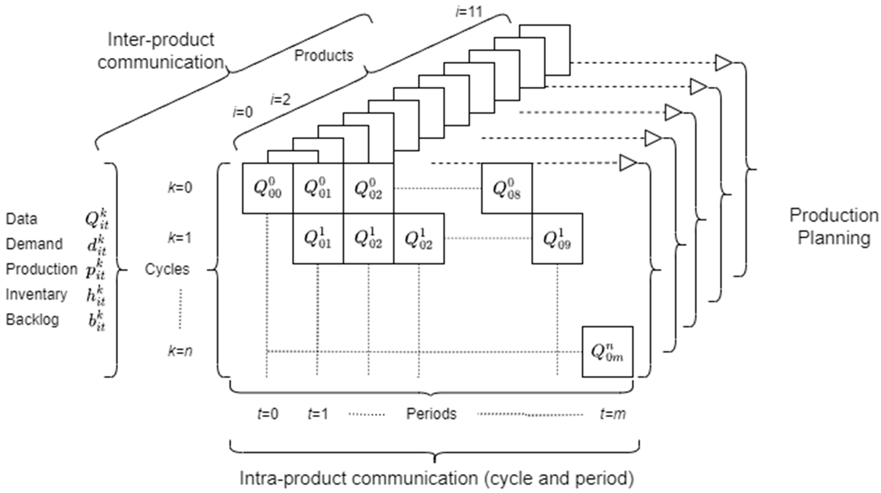
3.2. Measurement of System Nervousness

Nervousness measures the difference in the quantity of product $i$ to be produced in period $t$ during production cycle $k$ compared to the previous cycle and period. The calculation is based on two parameters (the magnitude of change and the frequency of changes), so significant changes or a high frequency of changes in production imply high values of nervousness. Two metrics express the nervousness per cycle and period. Let $C_{ki}$ be the number of schedule changes of product $i$ in cycle $k$ and $C_{ti}$ be the number of schedule changes of product $i$ in period $t$. Furthermore, let $Q_{it}^k$ be the production quantity for product $i$ in period $t$ in cycle $k$. Then, in Equation (6), $N_{cki}$ is the nervousness in cycle $k$ for product $i$, and in Equation (7), $N_{pti}$ is the nervousness in period $t$ for product $i$. Equation (8) presents the measure of nervousness $N$.

$$N_{cki}=C_{ki}\ast \left\{{\displaystyle {\sum }_{t=0}^{n-1}}{|Q}_{i\left(t+1\right)}^k{-Q}_{it}^k|\right\},\mathrm{Ɐ}k, \mathrm{Ɐ}i$$

(6)

$$N_{pti}=C_{ti}\ast \left\{{\displaystyle {\sum }_{t=0}^n}{|Q}_{it}^{\left(k+1\right)}{-Q}_{it}^k|\right\},\mathrm{Ɐ}t, \mathrm{Ɐ}i$$

(7)

$$N=N_{cki}+N_{pti}$$

(8)

Thus, $Q_{it}^k$ represents the quantity of production for product $i$ in period $t$ in cycle $k$. For the example in

Table 1. Example of production scheduling with a rolling horizon.

k/t	1	2	3	4	5	6	7	8
1	$Q_{i1}^1$	$Q_{i2}^1$	$Q_{i3}^1$	$Q_{i4}^1$
2		${\mathit{Q}}_{\mathit{i}\mathbf{2}}^{\mathbf{2}}$	${\mathit{Q}}_{\mathit{i}\mathbf{3}}^{\mathbf{2}}$	${\mathit{Q}}_{\mathit{i}\mathbf{4}}^{\mathbf{2}}$	${\mathit{Q}}_{\mathit{i}\mathbf{5}}^{\mathbf{2}}$
3			$Q_{i3}^3$	$Q_{i4}^3$	${\mathit{Q}}_{\mathit{i}\mathbf{5}}^{\mathbf{3}}$	$Q_{i6}^3$
4				$Q_{i4}^4$	${\mathit{Q}}_{\mathit{i}\mathbf{5}}^{\mathbf{4}}$	$Q_{i6}^4$	$Q_{i7}^4$
5					${\mathit{Q}}_{\mathit{i}\mathbf{5}}^{\mathbf{5}}$	$Q_{i6}^5$	$Q_{i7}^5$	$Q_{i8}^5$

, in period 5, nervousness is measured between ${\mathit{Q}}_{\mathit{i}\mathbf{2}}^{\mathbf{2}}$, ${\mathit{Q}}_{\mathit{i}\mathbf{3}}^{\mathbf{2}}$, ${\mathit{Q}}_{\mathit{i}\mathbf{4}}^{\mathbf{2}}$, and ${\mathit{Q}}_{\mathit{i}\mathbf{5}}^{\mathbf{2}}$ for $N_{cki}$ and ${\mathit{Q}}_{\mathit{i}\mathbf{5}}^{\mathbf{2}},{\mathit{Q}}_{\mathit{i}\mathbf{5}}^{\mathbf{3}},{\mathit{Q}}_{\mathit{i}\mathbf{5}}^{\mathbf{4}},$ and ${\mathit{Q}}_{\mathit{i}\mathbf{5}}^{\mathbf{5}}$ or $N_{pti}$.

The parameter ${\Phi }_k$ quantifies the ratio between cost and nervousness for each cycle k. In cycle k, $c\left(k\right)$ represents the cost and $N\left(k\right)$ represents the nervousness. This parameter identifies the magnitude of the change in each cycle by calculating the area under the curve of cost and nervousness. In addition, let c = [$c_1,\dots ,c_k$] and N= [$N_1,\dots ,N_k$] be two vectors to update ${\Phi }_k$; thus, ${\Phi }_k,k=\mathrm{1,2},\dots ,60$ is given by Equation (9).

$${\Phi }_k=\left|\frac{\sum _{k=1}^{k}c\left(k\right)}{\sum _{k=1}^{k}N\left(k\right)}\right|,\forall k\in \{k=1,\dots ,k=60\}$$

(9)

The following numerical example for k = 10 illustrates the updating of Equation (9). Considers values for c and N as follows:

c = [12.1, 12.44, 12.85, 13.34, 13.97, 14.6, 15.39, 16.3, 17.12, 18.05],

N = [1.79, −3.47, −8.63, −14.07, −19.13, −24.43, −29.74, −34.54, −38.87, −43.37].

Such values indicate that a program costing 12.1 monetary units has a nervousness of 1.79 for k = 0. Thus, the calculations of Φ are exemplified below for the vectors c and N.

$$\Phi =[\left|\frac{12.1}{1.79}\right|=6.76, \left|\frac{24.54}{-1.68}\right|=14.61,\left|\frac{37.39}{-10.3}\right|=3.63, \dots ,\left|\frac{128.1}{-171.1}\right|=0.75, \left|\frac{146.2}{-214.5}\right|=0.68]$$

3.3. PDS Architecture

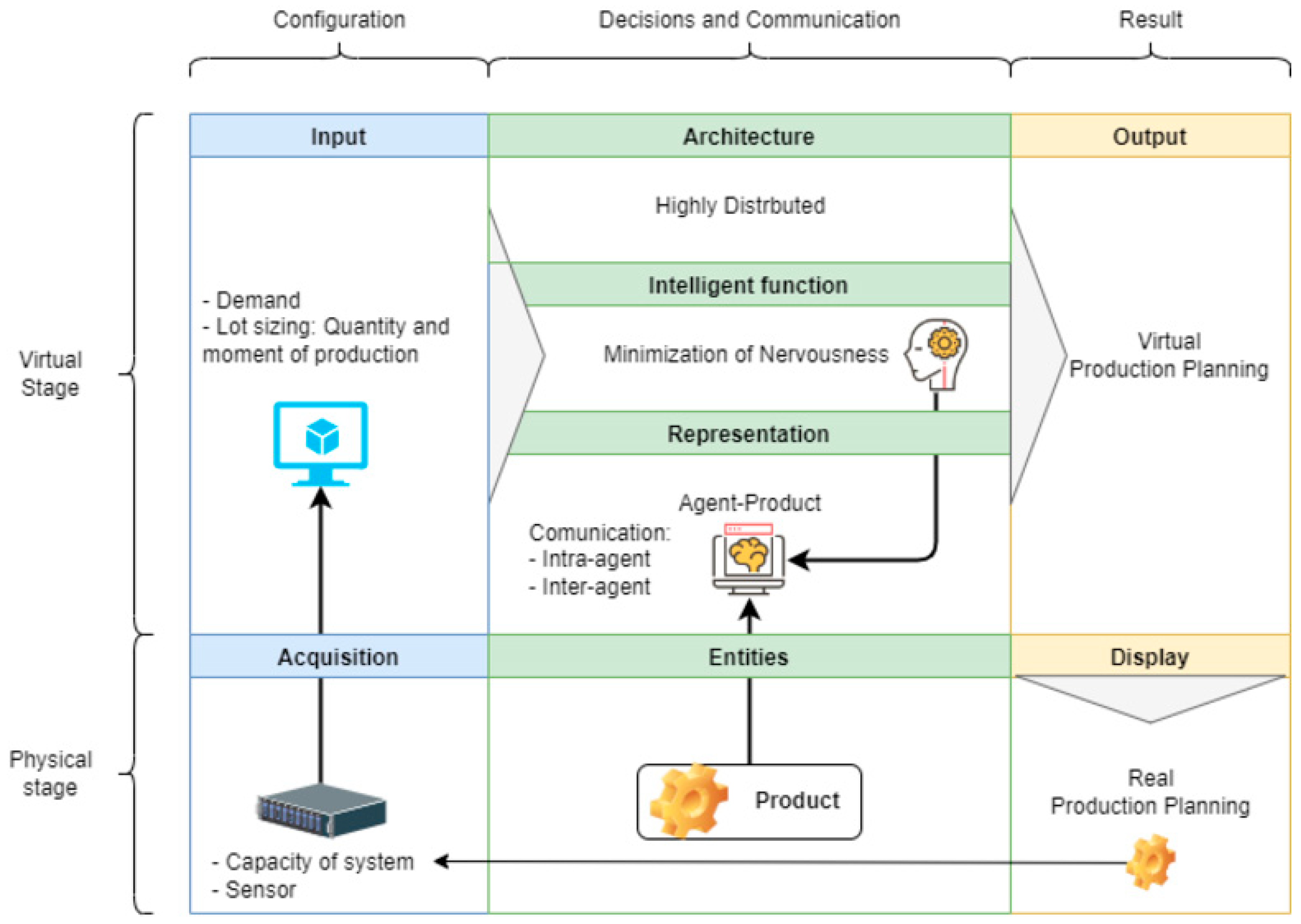
The system architecture contains physical and virtual layers, each with three levels (configuration, interactions, and results), as shown in Figure 1. An agent represents each product in the virtual layer, transforming the information into valuable data for decision making. The configuration of the virtual layer represents the results generated by the optimization model as data for communication and decision making by each agent. Thus, the physical layer of the system interacts with other physical entities, and its virtual layer interacts with the environment for production control and management. Decision making and communication among agents are distributed on the same hierarchical scale. The intelligence function of the agents considers decision rules for obtaining a global objective considering all of the system’s entities. Such decision rules are known and applied by all of the agents of the system through internal and inter-agent communication. This information is processed and stored in the physical part of the components. At the results level, the model outputs correspond to the production planning, virtually and physically representing the planning.

The virtual layer in Figure 1 contemplates an intelligence function that evaluates individual and collective performance, looking for system stability with a sustained cost increase. To this end, the intelligence function measures the nervousness of each agent using Equation (8). Each agent complies with the characteristics of an intelligent product defined by Wong et al. [43], i.e., they have a unique identifier and can communicate with the surrounding agents of the same product type.

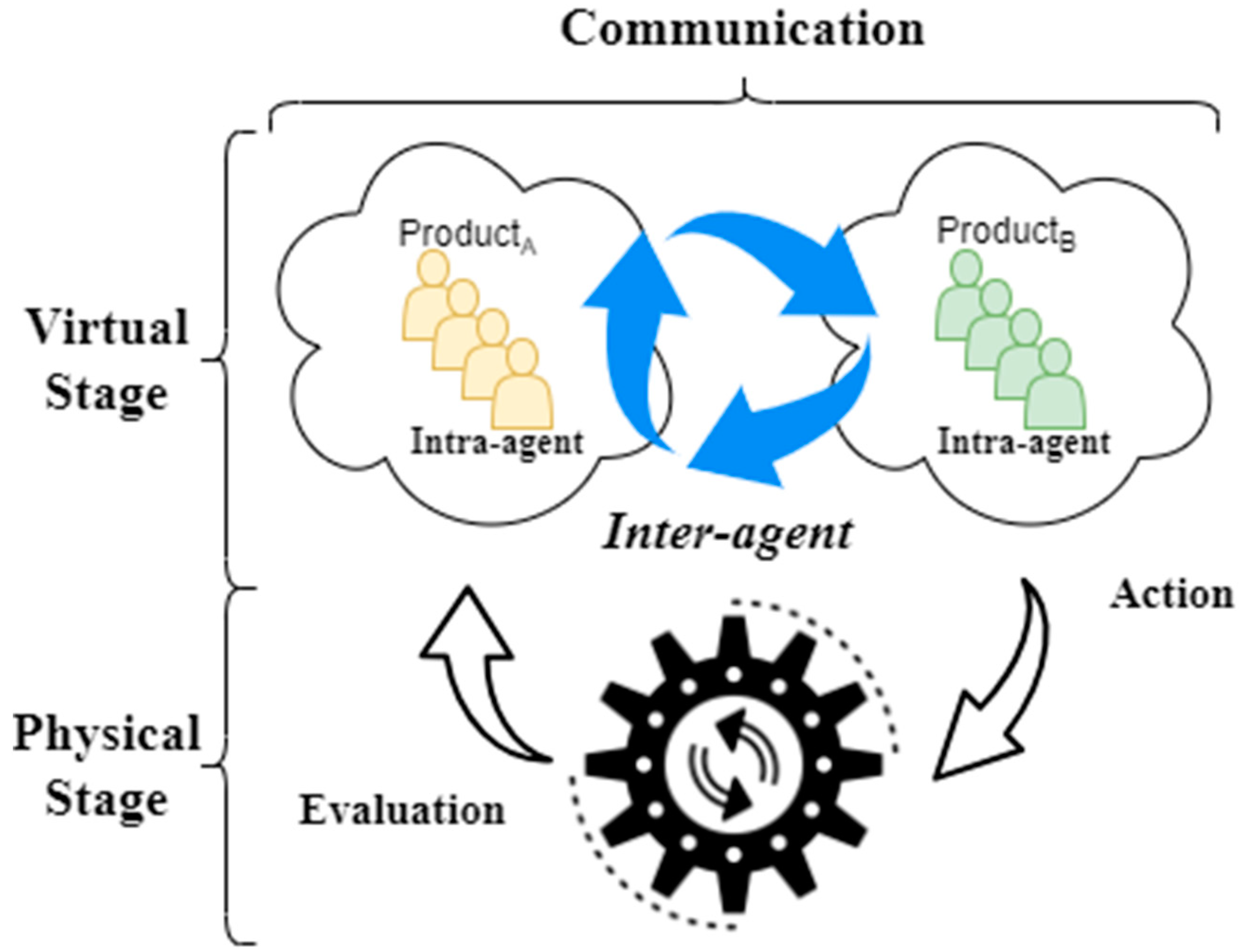
Agent communication occurs within the system’s virtual layer, where each product corresponds to an individual agent (Figure 1). This communication converts information into data. Each agent collects and processes data on its current state, production requirements, and resource needs. Interaction between agents occurs through a question-and-answer system. In addition, communication between agents eventually involves transferring data through the system optimization model, including results derived from production planning, capacity, and constraint information and recommendations to support decision making.

Figure 2 depicts the communication process among agents representing various product types within the system. These agents engage in virtual interactions, inquiring about the required production quantity for each period and cycle. Furthermore, when the daily production capacity is exceeded, agents reach out to agents representing other product types. Such interactions constitute internal communication among agents of the same type and external communication between agents of different types. For instance, an agent positioned in the production plan’s second cycle and second period would query the production quantities for future periods pertaining to the product it represents. Additionally, this agent would refer to the quantities produced in previous cycles to ensure production stability. This continuous communication facilitates the coordination of production activities and enables informed decision making that aligns with each product’s specific needs and capacities.

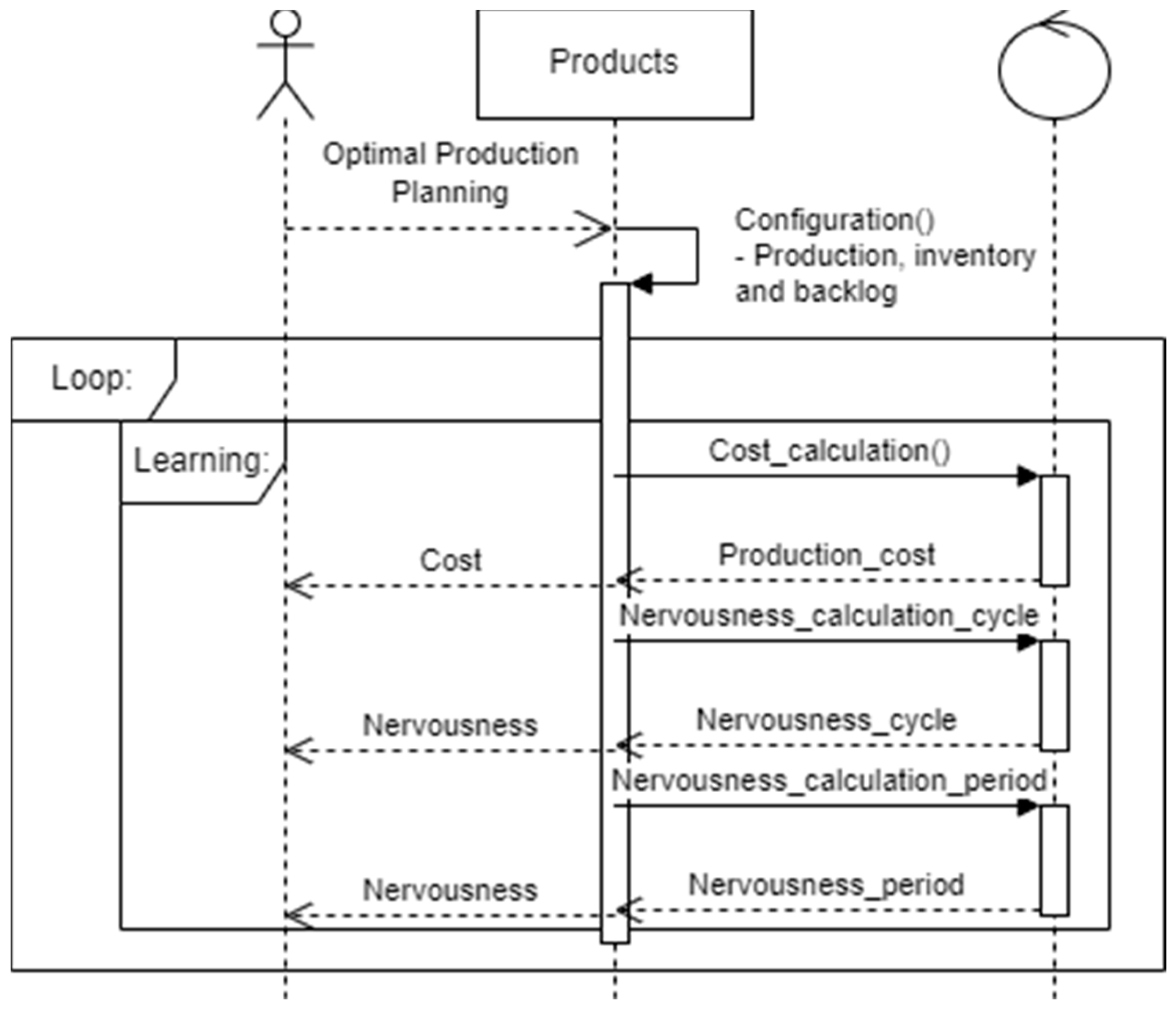
Figure 3 shows the sequence of actions of the proposed architecture. First, the algorithm solves the mathematical model and generates the optimal production. Then, the agents evaluate the nervousness and the planning cost to determine the required production that minimizes the increase in production cost. The objective function of the lot-sizing model (Equation (1)) is the basis of such calculation. Finally, agents communicate with other agents of the same product type in the corresponding cycle and period to evaluate the production quantity. Simultaneously, agents communicate with agents of another product family to avoid exceeding the system’s production capacity and to satisfy each product’s demand (see Figure 4). Then, the possibilities of decreasing nervousness are evaluated by modifying the production quantities and calculating the costs associated with such modifications. When a production quantity modification occurs that improves the value of nervousness, the agents store the production values. This communication architecture and these agent interactions respond to a perturbation of the system because of the permanent evaluation of quantities.

The production plan considers 12 products and a production horizon of 52 periods. The planning horizon is $n=8$ with an interval between periods of $\mathsf{\Delta }t=1$. The demand for each product obeys a normal distribution $d_{it}^k~\eta \left(\mathrm{\mu },\rho \right)=\eta \left(120,12\right),\mathrm{Ɐ}i,\mathrm{Ɐ}t,\mathrm{Ɐ}k$ to simulate different variations. The first stage outputs a master production plan for each product in the active period and a demand projection for subsequent periods. The complete simulation is set up with parameters that resemble a real industrial case, allowing a realistic evaluation of the model’s performance. Version 6.2 of the NetLogo simulation platform simulates the scenario providing a suitable environment for testing and monitoring model performance [52].

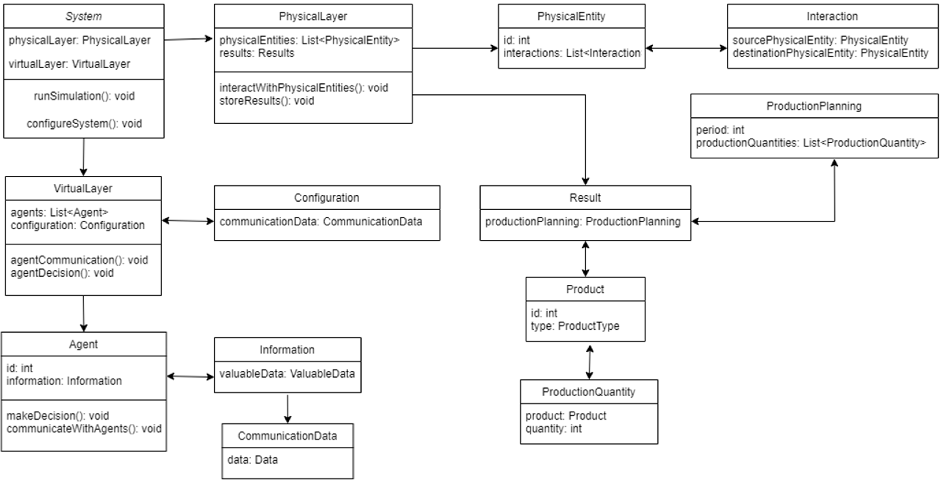
Figure 5 shows a class diagram to provide a reference model. The system contains a main class called “System”, which has two attributes: “PhysicalLayer” and “VirtualLayer”. The physical layer (“PhysicalLayer”) has a list of physical entities (“PhysicalEntity”) and a results attribute (“Results”). In addition, the virtual layer (“VirtualLayer”) has a list of agents (“Agent”) and a configuration (“Configuration”). Each physical entity and agent has its specific attributes and methods. The physical entities interact through the “Interaction” class, which registers the source and target physical entity. Agents make decisions and communicate with each other using the “Information” class to share valuable data. The “Results” class stores the production planning (“ProductionPlanning”), which has information about the period and production quantities for each product (“Product”) in the form of “ProductionQuantity” objects. In addition, the “CommunicationData” class manages the necessary communication data in the virtual layer.

4. Results

The PDS presents an initial phase of significant variation in cost and nervousness until it reaches a steady state. This phenomenon emerges from a simulation with three control variables: per period, per cycle, and per period cycle. In period control, intelligent products monitor production quantities during each period and modify the production plan to reduce nervousness. In cycle control, intelligent products control production quantities over the planning horizon. In period–cycle control, intelligent products look for period and cycle stability by considering consecutive periods of the planning horizon. In each type of control, Equations (6)–(8) update the nervousness.

Table 2. Analysis of percentage increase in the cost of the master production plan.

		Increase in Production Plan Cost
		1%	2%	3%	4%	5%	6%	7%	8%	9%	10%
% Reduction in nervousness	Cycle control	1.78	7.43	10.12	12.83	14.72	16.85	18.99	21.86	23.86	25.93
	Period control	42.41	51.71	56.98	61.89	63.8	67.08	68.63	69.72	71.7	72.97
	Cycle and period control	14.31	24.59	34.44	43.25	55.92	64.18	88.74	95.3	98.5	98.61

shows the results of analyzing the percentage increase in production costs up to 10%. Our model, with a 1% cost increase, reduces nervousness by 1.78%, 42.41%, and 14.31% in terms of cycle control, period control, and cycle–period control, respectively. This reduction in nervousness is consistent across the studied percentage increases, with period control being the most effective until a 6% cost increase. For cost increases exceeding 7%, cycle–period control becomes more effective, resulting in a 98.61% reduction in accumulative nervousness.

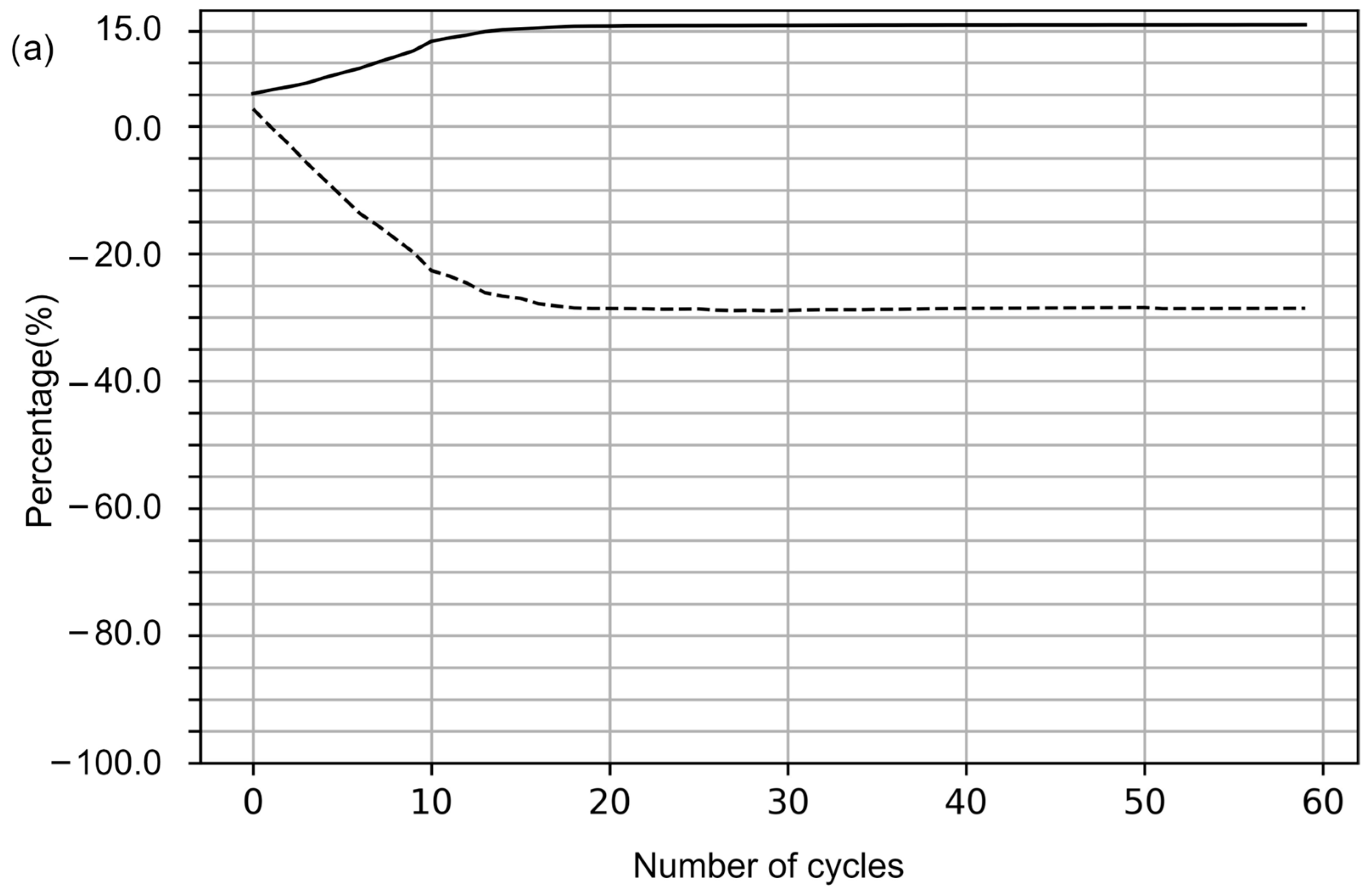
However, it is necessary to analyze the three types of control, evaluating the number of cycles required to reduce nervousness expressed in Table 2. Figure 6 shows the results of the cost and nervousness variations for each control type. The decrease in nervousness occurs with the consequent increase in cost concerning the initial values. For example, considering control by period (Figure 6a), there is an increase in cost of 11.21% and a reduction in nervousness of 14.72% in the eighth cycle. In control by cycle (Figure 6b), an increase in cost of 2.39% and a reduction in nervousness of 18.27% are observed. 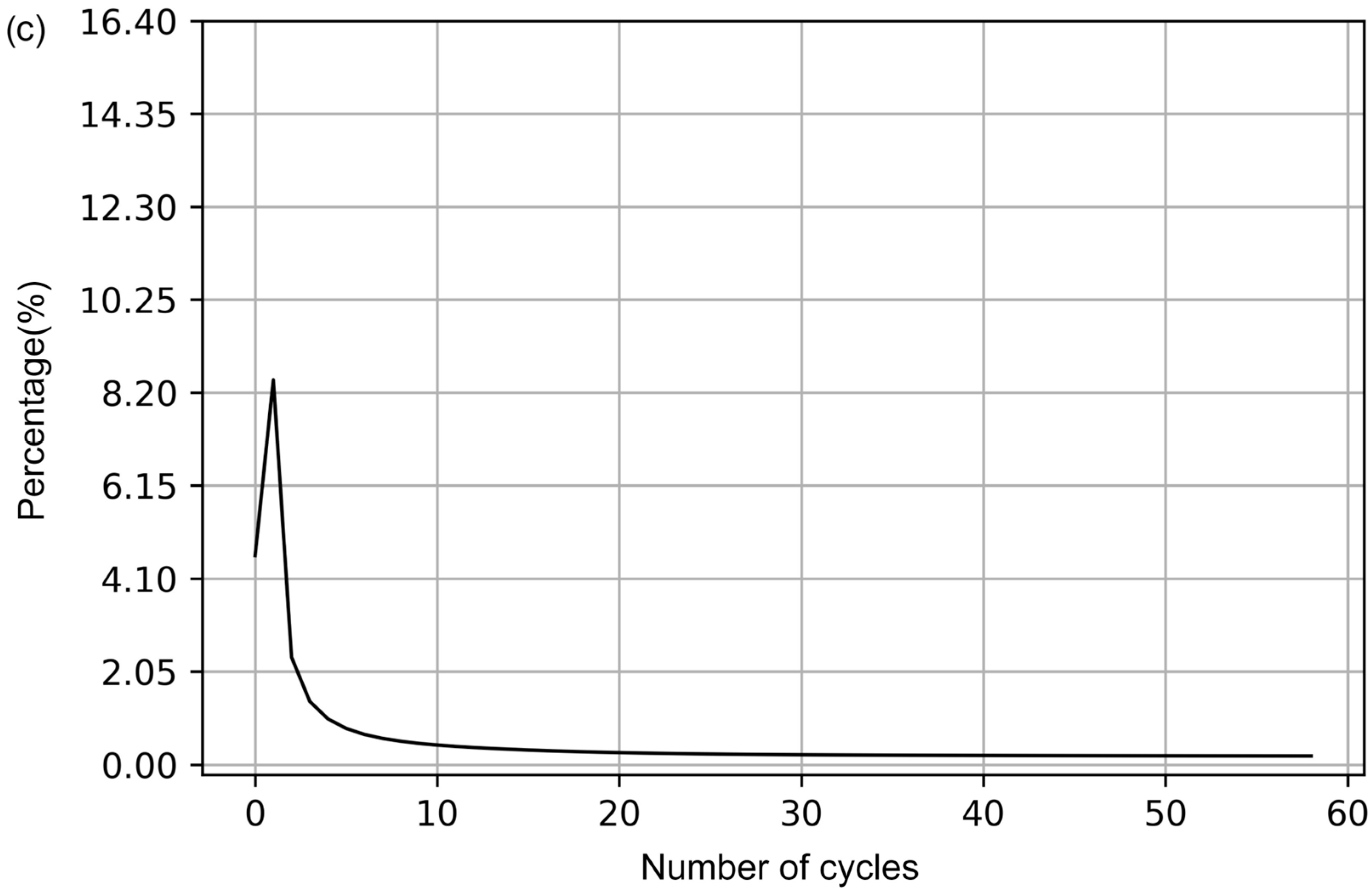Figure 6c shows the behavior of the PDS according to the period–cycle control. A more significant decrease in nervousness is observed than with the two types of controls. In the same programming cycle, an increase in cost of 11.27% and a reduction in nervousness of 34.44% are observed.

5. Discussion

The PDS results indicate an uneven relationship between decreased nervousness and increased costs. The more significant the decrease in nervousness, the smaller the increase in the cost of the production plan. This system-generated dynamic is consistent with the plan modification that minimizes the cost. In other words, any change in the production plan calculated through the mathematical model generates an increase in cost. However, the benefit of such a modification implies more stable plans. As the production cycles proceed, both cost and nervousness reach an equilibrium because modifying production quantities is no longer possible. 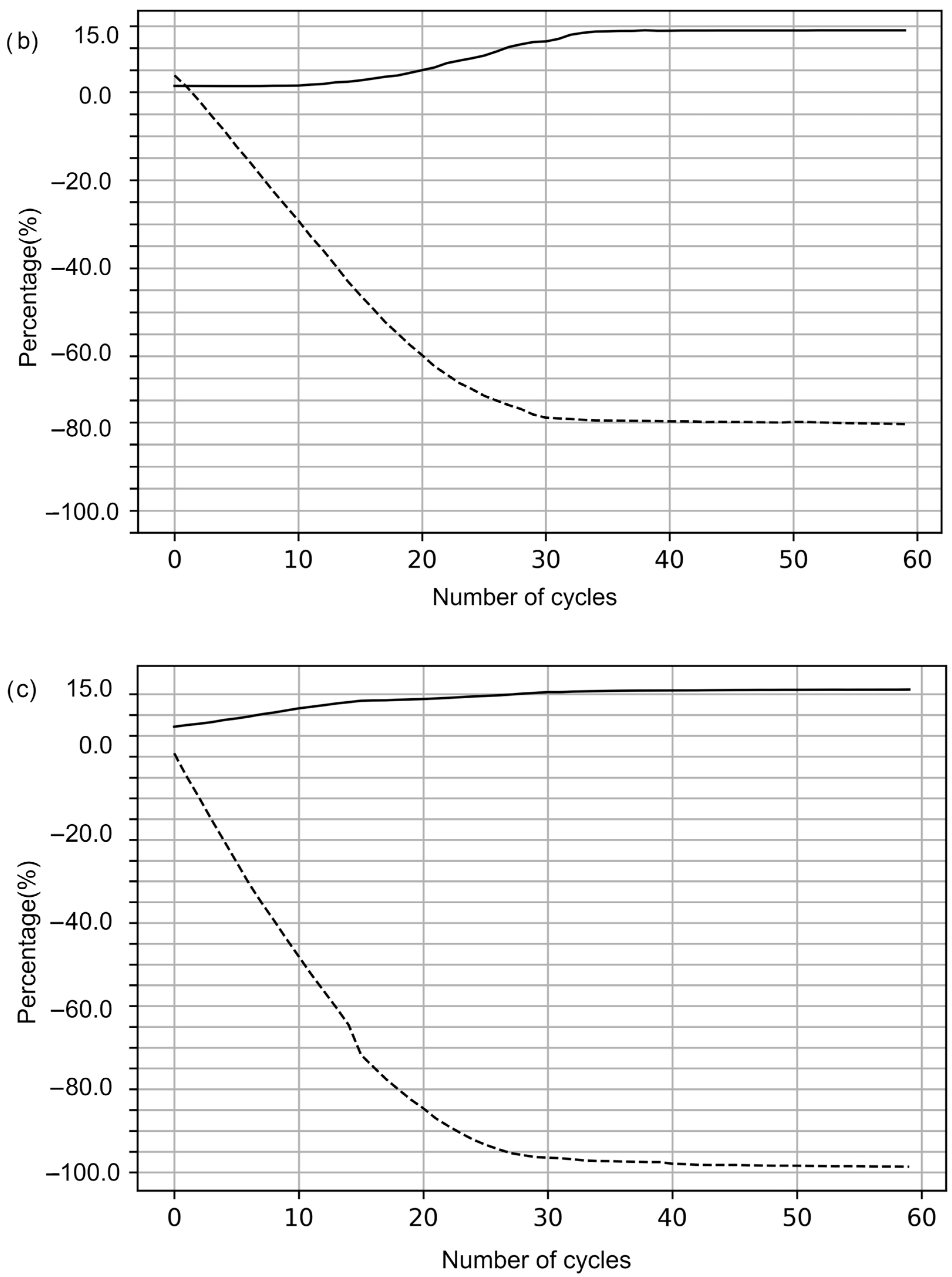Figure 7a–c show that the main results of decreasing nervousness and increasing cost occur before production cycle 10. In Figure 7, we observe the results for different values of ${\mathsf{\Phi }}_k$, which compare the initial cost increase with the benefits of nervousness reduction. The behavior is similar in the three types of control applied, obtaining a more noticeable change when using the cycle–period control, which optimizes in a balanced way between cycle and product.

In all types of control, cost increases with decreasing nervousness are observed in the first cycles of the simulation. However, after this initialization stage, a period of stability is reached during which there are no substantial differences in the magnitude of the changes associated with costs and nervousness. The computational results suggest that using a PDS is promising in reducing nervousness without substantial increases in production costs. Thus, a PDS can improve the master production plan by minimizing nervousness and adapting to changing environments.

The proposed system reduced uncertainty by 11.42% for the case study conducted. This is a promising result since uncertainty can be detrimental to production planning. However, a 2.39% increase in production costs was observed. In this case, the increase in production costs could be considered relatively low, especially considering the benefit of more accurate and stable planning. It is essential to consider that cost-effectiveness analysis may vary according to each production system’s context and specific priorities. Some companies may accept a slight cost increase if it implies stability in production and a significant reduction in uncertainty. Other companies may prioritize cost minimization and be less willing to accept additional increases. Thus, the precise assessment of cost-effectiveness depends on each company’s specific objectives and priorities.

6. Conclusions

This work proposes a production planning system that addresses nervousness management in production systems. The system utilizes intelligent products and starts from an initial production plan for the planning period generated through a mathematical cost minimization model. The numerical evaluation of the proposed system using a 12-product production system and a one-year planning period shows that it effectively reduces nervousness without significantly increasing production costs. For example, using cycle control, a modest increase in cost of 2.39% results in a significant reduction in nervousness of up to 11.42%.

The developed system includes a mathematical model, a metric for measuring uncertainty, and a definition of intelligent products. It is worth noting that there are several options and variants in the literature for each component, allowing for customization based on the specific needs of different industries. Future research could further explore these combinations of possibilities to develop production planning control systems tailored to industry-specific requirements.

It is relevant to emphasize that the proposed system generates flexible solutions without requiring multiple executions of a mathematical model, thus avoiding the resolution of computationally slow problems. This approach enables improved decision making in the modern industry by leveraging real-time process data that feed algorithms optimizing resource utilization. In turn, this fosters the development of a more sustainable industry, contributing to the innovation of new perspectives for uncertainty management in production planning.

Integrating new technologies into conventional manufacturing management is revolutionizing the industry, primarily to address challenges arising from demand fluctuations and operational disruptions. Product-driven production systems emerge as a promising solution by incorporating intelligent products capable of autonomous decision making and adaptation to disruptions. This approach enables more flexible planning, reduces nervousness, and mitigates increases in production costs. By implementing these approaches based on artificial intelligence and holonic systems, efficient solutions for production planning can be achieved across various industries. This integration enhances adaptability and optimizes resource allocation in sustainable manufacturing environments.

Overall, the findings of this study demonstrate the potential of using a production planning system to manage uncertainty in production planning, resulting in enhanced system performance in terms of reducing uncertainty and optimizing production costs. This work contributes to the existing literature on production planning and lays the groundwork for future research in this field.

As a future research direction, we propose exploring novel forms of embedded intelligence to improve response times and outcomes. These new forms would align with heuristics or machine learning techniques. In addition, it is possible to consider dynamism in the agent decision making, including functionalities that allow selecting the best decision at each moment according to different optimization criteria. Further study would determine the level of dynamism that does not exceed a certain threshold of computational time. Furthermore, expanding our study and considering real-world industrial cases is recommended. This would provide a more comprehensive understanding of the applicability and effectiveness of the proposed approach in diverse production environments.