Hardware Suitability of Complex Natural Resonances Extraction Algorithms in Backscattered Radar Signals

Abstract

Complex natural resonances (CNRs) extraction methods such as matrix pencil method (MPM), Cauchy, vector-fitting Cauchy method (VCM), or Prony’s method decompose a signal in terms of frequency components and damping factors based on Baum’s singularity expansion method (SEM) either in the time or frequency domain. The validation of these CNRs is accomplished through a reconstruction of the signal based on these complex poles and residues and a comparison with the input signal. Here, we perform quantitative performance metrics in order to have an evaluation of each method’s hardware suitability factor before selecting a hardware platform using benchmark signals, simulations of backscattering scenarios, and experiments.

1. Introduction

In 1971, Baum proposed the singularity expansion method (SEM) in which a time domain radar backscattered signal can be approximated as a sum of damped exponentials and complex residues [1,2]. He noticed how the frequencies (or poles) associated with these damped exponentials did not depend on the orientation of the object, and this led to the object identification as the poles can be used as its unique signature. Equation (1) shows how the input signal $y\left(t\right)$ is constructed with the complex residues $R_i$ and the poles $s_i$, having M as the number of complex natural resonances (CNRs). The poles $s_i={\alpha }_i+j{w}_i$, which are called the natural resonances of the object, represent the natural frequencies of the illuminated target [3,4]. In [5], SEM is mentioned as a useful method for determining experimental CNR of complex targets other than thin wires.

$$y\left(t\right)\approx \sum _{i=1}^M{R}_i{e}^{-s_{i}t}$$

(1)

The singularities in the time or frequency domain can be calculated using methods such as matrix pencil method (MPM), Prony’s method, Cauchy’s method, or vector-fitting Cauchy method (VCM) [6,7,8,9,10,11,12]. However, besides VCM, there is no reconstruction of the signal validated through numerical results that validate the poles for object identification scenarios or any analysis for real-time implementation. The main reason for this article is, then, to provide an insight into the advantages and disadvantages of each algorithm for several scenarios to extract useful information with the right procedure, and also obtain performance metrics such as execution time, number of samples, and accuracy. These metrics can subsequently serve as a basis for the selection or design of a hardware platform that conforms to the desired levels of accuracy, execution time, and number of samples required by the application.

In Section 2, the CNRs calculation methods are presented. Then, Section 3 describes the simulation and experimental setup, and after that we present the comparison of the results and discuss accuracy, execution time, and overall suitability for a hardware implementation.

2. Complex Natural Resonances Methods

2.1. Prony’s Method

In order to resolve a nonlinear problem, R. Prony proposed a method back in 1795 where a linear prediction equation is formed with an unknown coefficient vector and, before the amplitudes can be retrieved from the sample set, the frequencies are obtained from the roots of the prediction coefficient vector. Several modifications to this method have been proposed to increase its SNR [9,13], some used for SEM poles extraction and based on linear prediction (LP) for large data and presence of noise [14,15]. The least square (LS) and total least square (TLS) methods are applied as follows, using singular value decomposition (SVD) to lower the rank of the data matrix [16].

Starting with the linear prediction equation for a signal composed of complex sinusoids as in (2), Prony’s approach takes the data and their associated noise in the data matrix and the observation vector [17]. The linear prediction (LP) matrix (3) $Ab\approx g$ for data, the linear predictor, and the observation vector can be treated as if we were searching for the solution vector in the form of minimizing the $l_2$ norm for g.

$$y_n=\sum _{m=1}^p{c}_m{e}^{n{S}_{m}t}+W_{n}n=0,1,\dots ,N-1$$

(2)

$$\left[\begin{array}{cccc}{y}_{L-1}& y_{L-2}& \cdots & y_0\\ y_L& y_{L-1}& \cdots & y_1\\ ⋮& ⋮& \ddots & ⋮\\ y_{N-2}& y_{N-3}& \cdots & y_{N-L-1}\end{array}\right]\left[\begin{array}{c}{b}_0\\ b_1\\ ⋮\\ b_{m-1}\end{array}\right]=\left[\begin{array}{c}{y}_L\\ y_{L+1}\\ ⋮\\ y_{N-1}\end{array}\right]$$

(3)

The parameter L is an overestimate of the number of complex exponentials to compute from the data, and $b_m$ are the polynomial coefficients from which the poles are calculated with $b_0=1$. L is to be updated after a rank fix is applied, employing SVD.

The general description and steps for Prony’s algorithm are described in Figure 1 with the samples for the linear prediction (LP) matrix H, which becomes $H1$ after a rank fix using SVD.

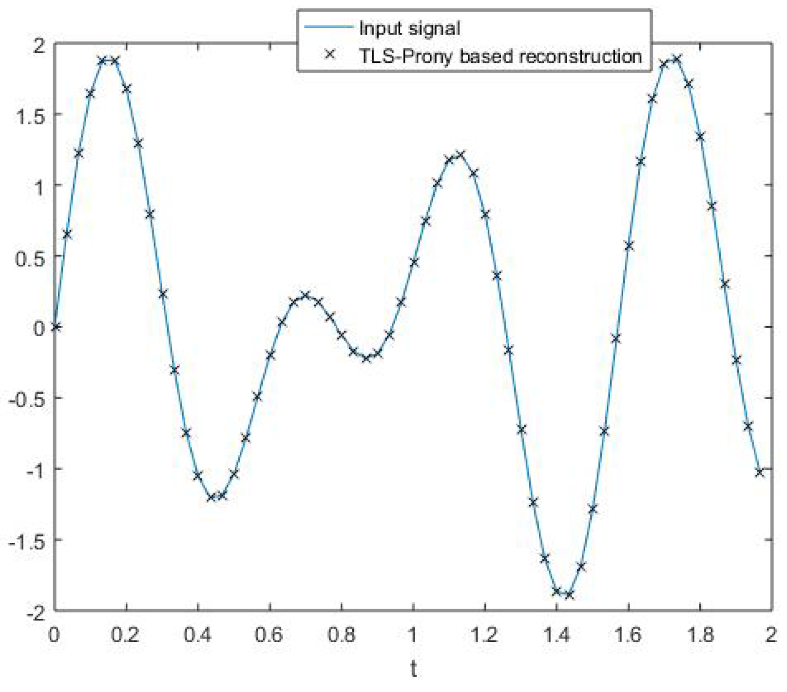
Now, as an example, a time series benchmark signal $y\left(t\right)=sin(8t+sin(12t\left)\right)$ is used to observe the behavior of this algorithm in terms of reconstruction accuracy after the poles have been found and the residues extrapolated. In Figure 2, the resulting approximation alongside the input time series is shown, and in Figure 3, the conjugated poles extracted with Prony’s method are presented.

2.2. Matrix Pencil Method

This method was presented in 1990 by [6] as an alternative method to Prony’s method for estimating parameters of backscattered signals with noise. It uses the pencil-of-function parameter, resulting in an improvement for noise sensitivity [6], and starts with Equation (4) for time domain samples and a discrete representation of the approximation of the input signal y into data samples $y_k$. This corresponds to a Hankel matrix $\left[Y\right]$ as in (5), with L as the pencil parameter, $k=1,2,\dots ,K$ the sample numbers, $z_n=e^{s_n{T}_s}$, the sampling period $T_s$, and $R_n$ the complex residues.

$$y_k\approx \sum _{i=1}^M{R}_n{z}_n^k$$

(4)

$$Y=\left[\begin{array}{cccc}{y}_o& y_1& \cdots & y_L\\ y_1& y_2& \cdots & y_{L+1}\\ ⋮& ⋮& \ddots & ⋮\\ y_{K-L-1}& y_{K-L}& \cdots & y_{K-1}\end{array}\right]$$

(5)

To find the critical components of (5), MPM uses $\lambda$ when Equation (6) is singular. This approach denotes $\left[Y_2\right]$ as the matrix $\left[Y\right]$ with the first column deleted and $\left[Y_1\right]$ as the matrix $\left[Y\right]$ with the last column deleted, and H as the Hermitian transpose. However, as the solution is not straightforward, several SVDs have to be computed from $\left[Y\right]$ to find $\lambda$ as follows.

$${\left[Y_2\right]}^H-\lambda {\left[Y_1\right]}^H$$

(6)

Applying SVD to $\left[Y\right]$ leads to (7) with $\left[U\right]$ having the largest n orthonormalized eigenvectors of $\left[Y\right]{\left[Y\right]}^H$, and $\left[V\right]$ the eigenvectors from ${\left[Y\right]}^H\left[Y\right]$. The singular values composing $[\Sigma ]$ are the nonnegative square roots of the eigenvalues of ${\left[Y\right]}^H\left[Y\right]$. After this matrix has been constructed, and assuming a noisy environment, a new matrix $\left[Y^{\prime }\right]$ and the corresponding $\left[U^{\prime }\right]$, $\left[{\Sigma }^{\prime }\right]$, and $\left[V^{\prime }\right]$ are defined, setting a minimum threshold in order to delete the nonzero and noise-dependent eigenvalues in $\left[Y\right]$.

$$\left[Y\right]=\left[U\right][\Sigma ]{\left[V\right]}^T$$

(7)

$$\frac{{\sigma }_M}{{\sigma }_{max}}={10}^{-p}$$

(8)

This threshold relies on the selection of a significance parameter, and a way to estimate it is to calculate the ratio between the maximum singular value and all others in the diagonal matrix $[\Sigma ]$ to obtain (8), with p being the number of significant decimal digits in the data [18].

Now that $\left[V^{\prime }\right]$ has M parameters, is separated into $\left[V_1^{\prime }\right]$ and $\left[V_2^{\prime }\right]$, where $\left[V_1^{\prime }\right]$ is $\left[V^{\prime }\right]$ with the last column deleted, and $\left[V_2^{\prime }\right]$ is $\left[V^{\prime }\right]$ with the first column deleted. Equation (6) could now have a singular solution for (9) with a reduced number of samples for the LP matrix.

$${\left[V_2\right]}^H-\lambda {\left[V_1\right]}^H$$

(9)

The SVD is used to compute the pseudo-inverse of ${\left[V_1\right]}^H$, which is then multiplied by ${\left[V_2\right]}^H$ to find the poles z. A least square approach will allow the determination of the residues R after a Vandermonde matrix is formed, as in Equation (10) [19].

$$\left[\begin{array}{c}{y}_o\\ y_1\\ ⋮\\ y_{K-1}\end{array}\right]=\left[\begin{array}{cccc}1& 1& \cdots & 1\\ z_1& z_2& \cdots & z_M\\ ⋮& ⋮& \ddots & ⋮\\ z_1^{K-1}& z_2^{K-1}& \cdots & z_M^{K-1}\end{array}\right]\left[\begin{array}{c}{R}_1\\ R_2\\ ⋮\\ R_M\end{array}\right]$$

(10)

The implementation of MPM is as shown in the block representation in Figure 4. There is a recursive step variables refinement and setup in which the reconstructed signal is compared with the input signal, and it also works as CNRs validation.

To test the accuracy of the CNRs extracted, a simple test is then carried out with the benchmark signal $y\left(t\right)=sin5t+sin10t$. Both the input signal and the pole-based reconstruction are compared, and the poles calculated through MPM are shown in Figure 5 and Figure 6, respectively.

2.3. Cauchy’s Method

In the frequency domain, this method was presented in 1821 by Cauchy, approximating a function by a ratio of two polynomials [20]. After that, it has been applied to the solution to electromagnetic problems modeling the system frequency response in the same way [11]. It assumes that the response is completely linear-time-invariant (LTI); thus, the transfer function can be written as in Equation (11) [10]. Equation (12) can be constructed with the coefficients $a_k$ and $b_k$ and then having $\left[C\right]$ as in Equation (13). As in the MPM approach, the SVD is applied to $\left[C\right]$ and a threshold to have the smallest singular value greater than or equal to the number of significant decimal digits of data in (14) and (15), having w as the number of accurate significant decimal digits in the data from the response.

$$H\left(f_i\right)\approx \frac{A\left(f_i\right)}{B\left(f_i\right)}=\frac{{\sum }_{k=0}^P{a}_k{f}_i^k}{{\sum }_{k=0}^Q{b}_k{f}_i^k},i=1,2,\dots ,N$$

(11)

$${[A-B]}_{N\times (P+Q+2)}{\left[\begin{array}{c}a\\ b\end{array}\right]}_{(P+Q+2)\times 1}={\left[C\right]}_{N\prod (P+Q+2)}{\left[\begin{array}{c}a\\ b\end{array}\right]}_{\times (P+Q+2)\times 1}=0$$

(12)

$$\left[C\right]=\left[\begin{array}{cccccccc}1& f_1& \cdots & f_1^P& -H_{f_1}& -H_{f_1}{f}_1& \cdots & -H_{f_1}{f}_1^Q\\ 1& f_2& \cdots & f_2^P& -H_{f_2}& -H_{f_2}{f}_2& \cdots & -H_{f_2}{f}_2^Q\\ ⋮& ⋮& \ddots & ⋮& ⋮& \ddots & ⋮\\ 1& f_N& \cdots & f_N^P& -H_{f_N}& -H_{f_N}{f}_N& \cdots & -H_{f_N}{f}_N^Q\end{array}\right]$$

(13)

$$\left[U\right][\Sigma ]{\left[V\right]}^H\left[\begin{array}{c}a\\ b\end{array}\right]=0$$

(14)

$$\frac{{\sigma }_R}{{\sigma }_{max}}\approx {10}^{-w}$$

(15)

Now, returning to (11), the TLS solution approach can be used to solve the equation and find the residues [19], which lead to the general steps for the method from the input signal to the reconstructed one in Figure 7.

A straightforward validation process occurs in the same way as the ones for MPM and Prony’s methods, but this time for a frequency domain benchmark signal $Y\left(\omega \right)=\frac{0.5}{\omega +1}+\frac{5}{\omega +5}+\frac{7}{\omega +6}+\frac{9}{\omega +8}$. The signal reconstruction comparison and the poles calculated with this method are shown in Figure 8 and Figure 9.

2.4. Vector-Fitting Cauchy Method

This approach is based on vector-fitting and Cauchy’s methods for calculating CNRs of a backscattered signal [10,12,21]. The VMC starts with the frequency domain signal treated as the response of the system $Y\left(s\right)$ and its transfer function approximation as a ratio of $u_k$ and $v_k$ coefficients, as in Equation (16). The solution to this system through a least square approach is the initial calculation of the poles of the system as in Cauchy’s method using the SVD as in Equation (17).

$$Y\left(s\right)=\frac{{\displaystyle \sum _{k=0}^P{u}_k{s}_i^k}}{{\displaystyle \sum _{k=0}^Q{v}_k{s}_i^k}}$$

(16)

$$\left[U\right]\left[S\right]{\left[V\right]}^{\prime }\left[\begin{array}{c}u\\ v\end{array}\right]=0$$

(17)

Then, these poles are treated as an initial guess for the system poles proposed in vector-fitting, which uses a partial-fraction expansion and a new function with the same poles as the input signal. The residues of this created signal $\widetilde{R_n}$ are the poles of the modeled signal, i.e., the calculated residues ${\tilde{R}}_N$ as the poles of the system. After this, Equation (18) can be used to find the solution with

$$f\left(s\right)=\sum _{n=1}^N\frac{R_n}{s-{\tilde{R}}_n}+d+sh.$$

(18)

The steps describing the VCM method are shown in Figure 10 and, again, a simple validation with a benchmark signal with known poles $Y\left(\omega \right)=\frac{0.8}{\omega +5}+\frac{3}{\omega +10}+\frac{9}{\omega +12}+\frac{10}{\omega +15}$ can be used for comparison and the poles location in Figure 10, Figure 11 and Figure 12.

3. Accuracy and Feasibility for Hardware Implementation

The approach for obtaining quantitative performance metrics for CNRs extraction methods is based on signal reconstruction accuracy, number of samples used, and execution time. For this, a set of backscattering signals in the time and frequency domain was obtained through simulations in CST Microwave Studio, experiments in free space, and buried objects in a sandbox.

The dimensions of the simulated objects are presented in

Table 1. Canonical objects simulated in three different positions.

	Dimensions (mm)
Thin wire	$l=100$, $d=2$
Sphere	$r=50$
Plate	$l_1=100,l_2=100,h=1$
Cylinder	$d=50,l=100,t=1$

, while the E-field vector was obtained in three different positions for every scenario. The backscattering response of a metal cylinder in free space was measured by using two RFSpace TSA600 antennas and a VNA. Likewise, the GPR measurements in a sandbox for buried objects are described in [22], where the EM responses for a metal plate and a metal can were obtained using Vivaldi antennas with operation frequencies from 0.8 GHz to 5 GHz.

In order to measure the accuracy of the reconstruction for each method, each backscattering signal is processed using MPM, Prony’s, Cauchy’s, and VCM algorithms, and the reconstruction validation is calculated with $R^2$ coefficient. A comparison of the number of samples used to compute the CNRs and the execution time will also provide a better insight into how these methods perform under different scenarios. This will provide a guide for an upcoming hardware implementation in a portable GPR.

3.1. Simulation Signals

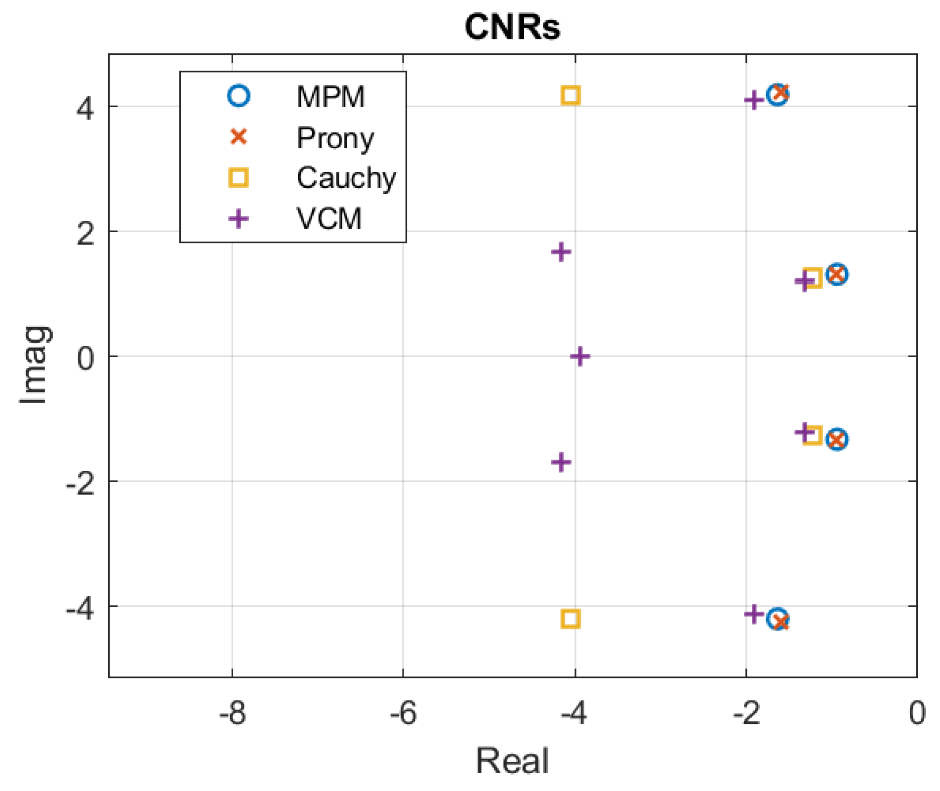
In Figure 13, the plots for the 100 mm length PEC thin wire response and its corresponding CNR-based reconstruction are shown. Subsequently, Figure 14 displays the CNRs in the complex plane. For time domain analysis, the signal processing is that of the late-time response of the object only; however, this part of the response is included in the frequency domain. Therefore, as the calculated CNRs do not have any filtering or preprocessing, they show similar characteristics but are not exactly the same. Considering this CNRs comparison, as the damping factor $\alpha$, which is the real part of each CNR, approaches zero, its contribution to the signal in the form of an exponential decay becomes more significant, and the complex conjugated component of the CNR is related to the oscillation frequency. This means that two main frequencies can be identified in Figure 14 with the imaginary values 1.45 and 4.26, which also correspond to the expected resonances for this particular thin wire.

3.2. Experimentally Registered Signatures

To measure an aluminum cylinder in free space, three responses from different positions were obtained using two low-cost TSA600 Vivaldi antennas from RFSpace with a VNA in the frequency range from 1 MHz to 3 GHz. The setup is shown in Figure 15 alongside the reconstruction-wise behavior of each method in Figure 16.

Now, as a critical evaluation requires the backscattered response of buried objects, a sandbox experiment was performed using an ultrawide band (UWB) radar from 0.8 GHz to 5 GHz and Vivaldi antennas as well [22]. As before, the time and frequency responses for a metal can and a metal plate were obtained and processed with complex natural resonances extraction methods (CNREMs), and the reconstruction of the signal is shown in Figure 17.

3.3. Methods Evaluation

Backscattered signals from simulation and experimentation were the input for CNREM reconstruction accuracy, using the minimum number of samples and the higher $R^2$ coefficient obtained. The execution time in a computer with an Intel Core i7 processor and 32 GB of RAM was calculated afterward for the 21 scenarios.

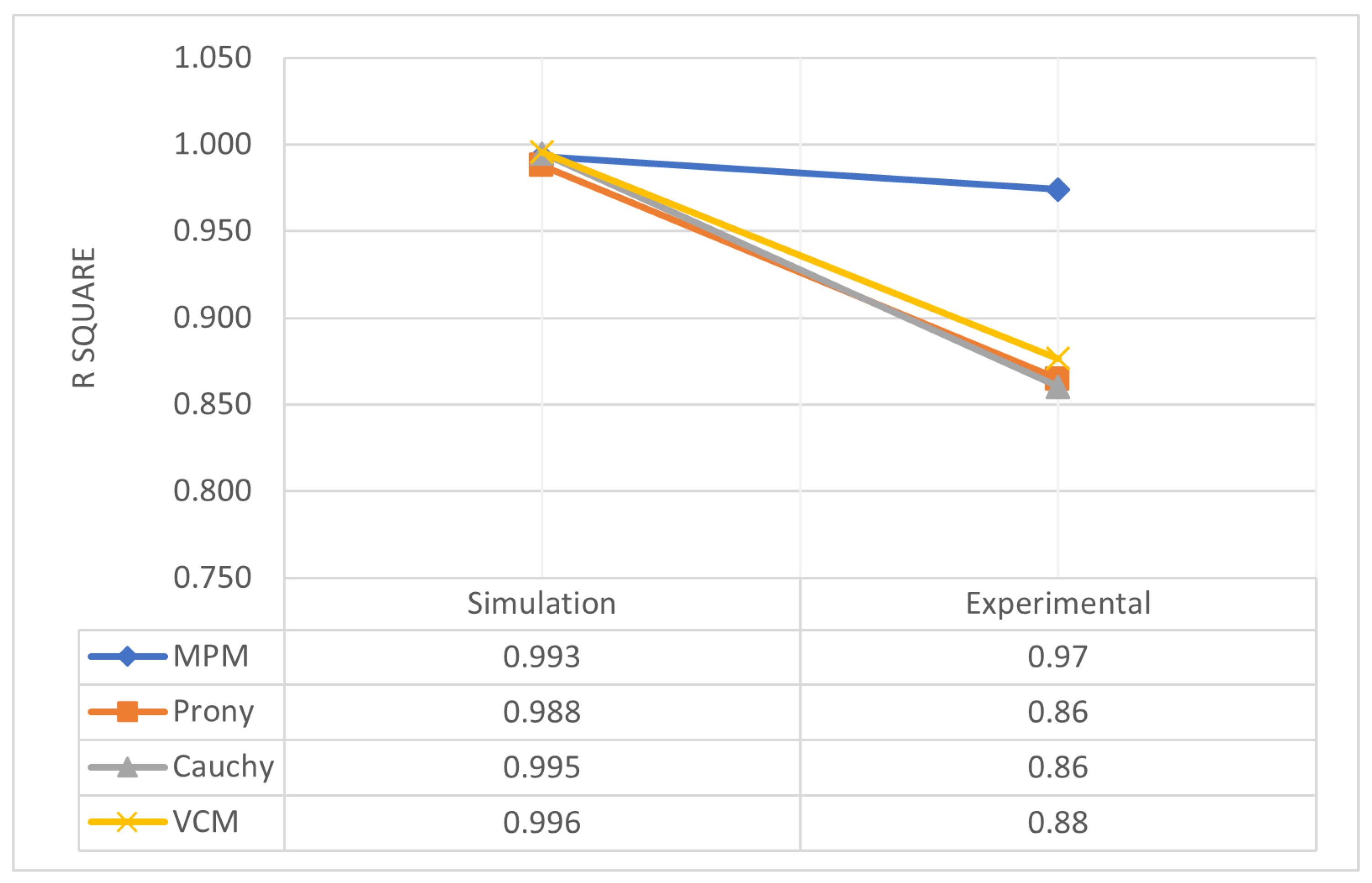
Now, the comparison starts with the accuracy of each method, i.e., the fidelity of the reconstruction. The CNRs calculated from the input signal are the base for the linear regression that leads to the signal reconstruction, so the CNRs calculated are reliable only if this reconstructed signal has a $R^2$ coefficient (from 0 to 1) close or equal to 1. The average for these measurements is presented in Figure 18, where MPM outperforms in both simulation and experimental scenarios.

When the higher $R^2$ for each signal was obtained, the number of samples for the linear prediction matrix in time or frequency domain methods were compared and are shown in Figure 19. Here, frequency domain methods (Cauchy’s and VCM) use significantly fewer samples to obtain an acceptable reconstruction. The execution time was the final approach for understanding CNREM as a signal processing tool feasible for hardware implementation in GPR operations. Figure 20 shows how time domain methods use, on average, less processing time than frequency domain methods.

Time domain methods have a better time performance than frequency domain methods, and MPM in particular has a good reconstruction, with the highest $R^2$ coefficient for experimental scenarios. However, for real-time implementation, the number of samples and the late-time response identification could use additional hardware resources. This consideration is not present in frequency domain methods.

3.4. Hardware Suitability

It is important to note that the relationship between these metrics can be highly problem-specific, having different trade-offs and considerations when it comes to execution time, number of samples, and accuracy. However, and only to offer additional perspective on the preceding analysis, an estimated hardware suitability factor (HSF) ${\psi }_{R^2}$ with $R^2$ as the accuracy measurement method can be considered, as in Equation (19). This factor could provide an initial measurement of how suitable a CNREM is for hardware implementation in a portable device.

Considering that this suitability factor decreases as time and the number of samples increase, and increases with accuracy, then ${\psi }_{R^2}$ is directly proportional to A and inversely proportional to N and $t_e$. In other words, ${\psi }_{R^2}\propto A_{R^2}\frac{1}{N}\frac{1}{t_e}$. This factor is meant to be dimensionless, so the time units have to be ignored.

$${\psi }_{R^2}=\frac{A_{R^2}}{N{t}_e}$$

(19)

The results, including all the experimental and simulated scenarios for the HSF, are shown in Figure 21. The frequency domain methods are more suitable for a hardware implementation, more specifically Cauchy’s method.

4. Conclusions

Several backscattering signals from objects in different positions and experiments with different schemes were presented and processed with Prony, matrix pencil method, Cauchy, and VCM in order to find the CNRs and then compare the reconstruction fidelity, number of samples used, and execution time, with the intention of having a better insight before selecting or designing a hardware platform for a particular study.

If high reconstruction accuracy, i.e., reliable CNRs extracted, is desired, MPM is the most appropriate choice with low execution time (assuming a previous identification of the late-time response). If a reduced number of samples to process is required by the signal acquisition hardware (or if the hardware capabilities are limited), then frequency domain methods should be considered instead. Additionally, VCM should be selected if buried targets are to be studied; this is because the reconstruction fidelity is better in experimental scenarios.

Prony’s method has a low $R^2$ coefficient with experimental signals, probably due to a low SNR, even though it employs the same number of samples as MPM, and for this reason, it is not recommended above the other methods studied here. However, according to the first approach of the HSF, Cauchy’s method should be implemented in hardware first.

If the hardware implementation of this signal processing technique requires a real-time operation or a portable device, such as a portable GPR, two approaches could follow. The first one is to increase the reconstruction quality of frequency domain methods, as the sample set to be processed is small, and also reduce the execution time. The second approach is to reduce the number of samples or MPM computation time (or hardware resources needed); however, these improvements are still to be studied. In future work, the hardware-suitability factor, including computational complexity, has to be tested in a digital platform, which can also include hardware acceleration.

References

- Baum, C.E. On the Singularity Expansion Method for the Solution of Electromagnetic Interaction Problems; Technical Report, DTIC Document; DTIC: Fort Belvoir, VA, USA, 11 December 1971. [Google Scholar]
- Baum, C.; Rothwell, E.; Chen, K.M.; Nyquist, D. The singularity expansion method and its application to target∖nidentification. Proc. IEEE 1991, 79, 1481–1492. [Google Scholar] [CrossRef]
- Lee, W. Identification of a Target Using its Natural Poles Using Both Frequency and Time Domain Response. Ph.D. Thesis, Syracuse University, Syracuse, NY, USA, 2013. [Google Scholar]
- Dolph, C.L. The Singularity Expansion Method and Complex Singularities of Exterior Scalar and Vector Scattering in Acoustics & Electromagnetic Theory. 1979. Available online: https://apps.dtic.mil/sti/citations/ADA215164 (accessed on 1 May 2023).
- Giri, D.V.; Tesche, F.M. An Overview of the Natural Frequencies of a Straight Wire by Various Methods. IEEE Trans. Antennas Propag. 2012, 60, 5859–5866. [Google Scholar] [CrossRef]
- Hua, Y.; Sarkar, T.K. Matrix Pencil Method for Estimating Parameters of Exponentially Damped/Undamped Sinusoids in Noise. IEEE Trans. Acoust. Speech Signal Process. 1990, 38, 814–824. [Google Scholar] [CrossRef]
- Sarkar, T.K.; Hu, F.; Hua, Y.; Wicks, M. A real-time signal processing technique for approximating a function by a sum of complex exponentials utilizing the matrix-pencil approach. Digit. Signal Process. 1994, 4, 127–140. [Google Scholar] [CrossRef][Green Version]
- Sarrazin, F.; Chauveau, J.; Pouliguen, P.; Potier, P.; Sharaiha, A. Accuracy of singularity expansion method in time and frequency domains to characterize antennas in presence of noise. IEEE Trans. Antennas Propag. 2014, 62, 1261–1269. [Google Scholar] [CrossRef]
- Rahman, M.A.; Yu, K.B. Total least squares approach for frequency estimation using linear prediction. IEEE Trans. Acoust. Speech Signal Process. 1987, 35, 1440–1454. [Google Scholar] [CrossRef]
- Lee, W.; Sarkar, T.K.; Moon, H.; Salazar-Palma, M. Computation of the natural poles of an object in the frequency domain using the cauchy method. IEEE Antennas Wirel. Propag. Lett. 2012, 11, 1137–1140. [Google Scholar] [CrossRef]
- Yang, J.; Sarkar, T.K. Interpolation/extrapolation of radar cross-section (RCS) data in the frequency domain using the cauchy method. IEEE Trans. Antennas Propag. 2007, 55, 2844–2851. [Google Scholar] [CrossRef]
- Gallego, A.; Roman, F.; Pineda, E. Vector Fitting—Cauchy Method for the Extraction of Complex Natural Resonances in Ground Penetrating Radar Operations. Algorithms 2022, 15, 235. [Google Scholar] [CrossRef]
- Prony, R. Essai experimental et analytique sur les lois de la dilatabilite des fluides elastiques et sur celles de la force expansive de la vapeur de leau et de la vapeur de lalkool, r differentes temperatures. J. Polytech. Bull. Trav. Fait Lecole Cent. Des Trav. Public Paris Prem. Cah. 1795, 1, 24–76. [Google Scholar]
- Tufts, D.; Kumaresan, R. Singular value decomposition and improved frequency estimation using linear prediction. IEEE Trans. Acoust. Speech Signal Process. 1982, 30, 671–675. [Google Scholar] [CrossRef]
- Makhoul, J. Linear Prediction: A Tutorial Review. Proc. IEEE 1975, 63, 561–580. [Google Scholar] [CrossRef]
- Householder, A.S. On Prony’s Method of Fitting Exponential Decay Curves and Multiple-Hit Survival Curves. 1950. Available online: https://www.osti.gov/biblio/4444525 (accessed on 1 May 2023).
- Golub, G.H.; Van Loan, C.F. An Analysis of the Total Least Squares Problem; Society for Industrial and Applied Mathematics: Philadelphia, PA, USA, 1980. [Google Scholar] [CrossRef]
- Sarrazin, F.; Sharaiha, A.; Pouliguen, P.; Chauveau, J.; Collardey, S.; Potier, P. Comparison between Matrix Pencil and Prony methods applied on noisy antenna responses. In Proceedings of the LAPC 2011-2011 Loughborough Antennas and Propagation Conference, Loughborough, UK, 14–15 November 2011. [Google Scholar] [CrossRef]
- Markovsky, I.; Van Huffel, S. Overview of total least-squares methods. Signal Process. 2007, 87, 2283–2302. [Google Scholar] [CrossRef]
- Cauchy, A.L. Sur la formule de Lagrange relative à l’interpolation. In Cours D’analyse de l’École Royale Polytechnique; Cambridge University Press: Cambridge, UK, 1821; pp. 525–529. [Google Scholar] [CrossRef]
- Gustavsen, B.; Semlyen, A. Rational Approximatin of Frequency Domain Responses by Vector Fitting. IEEE Trans. Power Deliv. 1999, 14, 1052–1061. [Google Scholar] [CrossRef]
- Gutierrez, S. Application of Time-Frequency Transformations in Polarimetric UltraWideband MIMO-GPR signals for Detection of Colombian Improvised Explosive Devices. Ph.D. Thesis, Repositorio Universidad Nacional, Bogota, Colombia, 2019. [Google Scholar]
Figure 1.
Prony’s method algorithm in a general step-by-step flow chart.
Figure 2.
Benchmark signal and Prony’s CNR-based reconstruction.
Figure 3.
Prony’s CNRs calculated.
Figure 4.
General steps for implementing MPM algorithm and comparing input and output signals for CNRs validation.
Figure 5.
Input signal and its reconstruction using the CNRs calculated through MPM.
Figure 6.
Poles calculated with MPM from the benchmark signal . These poles come in conjugated pairs in the complex plane.
Figure 7.
Generalized steps in Cauchy’s algorithm for finding the CNRs from an input signal, which is compared with the reconstructed one in the final step for validation purposes.
Figure 8.
Input signal and its reconstruction based on the poles and residues calculated through Cauchy’s method.
Figure 9.
Poles calculated through Cauchy’s method in the complex plane.
Figure 10.
VCM method for a frequency domain backscattered signal [
12].
Figure 11.
Input signal and its reconstruction based on the poles and residues calculated through the VCM method.
Figure 12.
Poles calculated using the VCM method, plotted in the complex plane.
Figure 13.
Thin wire time domain response for Prony’s based reconstruction, MPM, frequency domain response with Cauchy-based reconstruction, and VCM.
Figure 14.
Comparison of the CNR poles calculation of the simulated thin wire in the complex plane.
Figure 15.
Experimental setup for free space experiments and the metal cylinder with two Vivaldi antennas.
Figure 16.
Metal cylinder in free space. Prony reconstruction, MPM-based reconstruction, frequency response Cauchy method based reconstruction, and VCM reconstruction.
Figure 17.
Buried objects measurement in a sandbox. Time domain late-time response for Prony’s and MPM-based reconstructions, and frequency domain response for Cauchy’s and VCM reconstructions.
Figure 18.
comparison for CNREM in different scenarios.
Figure 19.
Average number of samples per CNREM in different scenarios.
Figure 20.
Execution time per CNREM.
Figure 21.
Average number of samples per HSF in different scenarios.