Applying Particle Swarm Optimization Variations to Solve the Transportation Problem Effectively

Abstract

The Transportation Problem (TP) is a special type of linear programming problem, where the objective is to minimize the cost of distributing a product from a number of sources to a number of destinations. Many methods for solving the TP have been studied over time. However, exact methods do not always succeed in finding the optimal solution or a solution that effectively approximates the optimal one. This paper introduces two new variations of the well-established Particle Swarm Optimization (PSO) algorithm named the Trigonometric Acceleration Coefficients-PSO (TrigAc-PSO) and the Four Sectors Varying Acceleration Coefficients PSO (FSVAC-PSO) and applies them to solve the TP. The performances of the proposed variations are examined and validated by carrying out extensive experimental tests. In order to demonstrate the efficiency of the proposed PSO variations, thirty two problems with different sizes have been solved to evaluate and demonstrate their performance. Moreover, the proposed PSO variations were compared with exact methods such as Vogel’s Approximation Method (VAM), the Total Differences Method 1 (TDM1), the Total Opportunity Cost Matrix-Minimal Total (TOCM-MT), the Juman and Hoque Method (JHM) and the Bilqis Chastine Erma method (BCE). Last but not least, the proposed variations were also compared with other PSO variations that are well known for their completeness and efficiency, such as Decreasing Weight Particle Swarm Optimization (DWPSO) and Time Varying Acceleration Coefficients (TVAC). Experimental results show that the proposed variations achieve very satisfactory results in terms of their efficiency and effectiveness compared to existing either exact or heuristic methods.

1. Introduction

The Transportation Problem (TP) is one of the most significant types of linear programming problems. The aim of the TP is to minimize the cost of transportation of a given commodity from a number of sources or origins (e.g., factory manufacturing facility) to a number of destinations (e.g., warehouse, store) [1]. Over the years, many classical and stochastic search approaches have been applied for the purpose of solving the TP.

The Northwest Corner method (NWC) is one of the methods that obtains a basic feasible solution to various transportation problems [2]. This process very easily allocates the amounts when few demand and destination stations exist. Moreover, frequently, the exported solution does not approach the optimal. The Minimum Cost Method (MCM) [3] is an alternative method which can yield an initial basic feasible solution. The MCM succeeds in lowering total costs by taking into consideration the lowest available cost values while finding the initial solution. An innovative approach comes from the Vogel Approximation Method (VAM); the VAM is an upgraded version of the MCM which results in a basic feasible solution close to the optimal solution [3]. Both of them take the unit transportation costs into account and obtain satisfactory results; however, VAM is rather slow and computationally intensive for a large range of values. Nevertheless, it has been proven that in problems with a small range of values and a relatively small number of variables, the above exact methods are quite efficient.

In some cases, TP has a complex structure, multifaceted parameters and a huge amount of data to be studied. Therefore, exact methods do not succeed in finding a suitable solution in an acceptable time period; a result, it is unpractical to use them. Taking into consideration the above, apart from conventional solution techniques, various heuristic and metaheuristic methods have been designed to capitalize on their potential capabilities. Specifically, metaheuristic algorithms attempt to find the best feasible solution, surpassing the other technique as much in terms of quality as in computational time [4]. Mitsuo Gen, Fulya Atliparmak and Lin Lin applied a Genetic Algorithm (GA) for a two-stage TP using priority-based encoding, showing that the GA has been receiving great attention and can be successfully applied for combinational optimization problems [5]. Ant Colony Optimization (ACO) algorithms have already proven their efficiency in many complex problems; they constitute a very useful optimization tool for many transportation problems in cases where it is impossible to find an algorithm that finds the optimal solution or in cases where the time interval does not make it possible to approve this solution [6]. The applications of hybrid methods with the combination of two or more heuristic, metaheuristic or even exact methods are also widespread. Interesting research was undertaken in 2019 by Mohammad Bagher Fakhrzad, Fariba Goodarzian and Golmohammadi [7]. In their study, four metaheuristic algorithms, including Red deer Algorithm (RDA), Stochastic Fractal Search (SFS), Genetic Algorithm (GA) and Simulated Annealing (SA), as well as two hybrid algorithms, the RDA and GA (HRDGA) algorithm and the Hybrid SFS and SA (HRDGA) algorithm, were utilized to solve the TP, demonstrating significant effectiveness [7].

Motivated by the above-mentioned applications of metaheuristic algorithms to cope with the TP, this work deals with the application of Particle Swarm Optimization (PSO) to solve the TP effectively. The PSO algorithm was first introduced by Dr. Kennedy and Dr. Eberhart in 1995 and was known as a novel population-based stochastic algorithm, working out complex non-linear optimization problems [8]. The basic idea was originally inspired by simulations of the social behavior of animals such as bird flocking, fish schooling, etc. Possessing their own intelligence, birds of the group connect with each other, sharing their experiences, and follow and trust the mass in order to reach their food or migrate safely without knowing in advance the optimal way to achieve it. The proposed research is expected to enhance the abilities of both the social behavior and personal behavior of the birds. It is observed that the original PSO has deficits in premature convergence, especially for problems with multiple local optimums [9]. The swarm’s ability to function with social experience as well as personal experience is determined in the algorithm through two stochastic acceleration components, known as the cognitive and social components [10]. These components have the aptitude to guide the particles in the original PSO method to the optimum point as the correct selection of their values is the key influence on the success and efficiency of the algorithm. Much research has been carried out with a focus on finding out the best combination of these components [10].

First, this paper examines approaches that have already been applied with great success to solve the TP. Adding to the above, two new PSO variations are presented and applied to solve the TP, operating proper transformations of the main PSO parameters. Experimental results show that these new PSO variations have very good performance and efficiency in solving the TP compared to the former methods.

In order to confirm the technical merit and the applied value of our study, 32 instances of the TP with different sizes have been solved to evaluate and demonstrate the performance of the proposed PSO variations. Their experimental results are compared with those of well-known exact methods, proving their superiority over them. One major innovation of the proposed variations is the appropriate combination of acceleration coefficients (parameters c₁, c₂) and inertia weight (parameter w) [11] (see Section 3) in order to come up with better computational results compared to existing approaches. Exhaustive experimental results demonstrate that the performance of the new PSO variations noted significantly higher performance not only compared to the exact methods already applied to solve the TP but also compared to the other PSO variations already introduced in the respective literature. Furthermore, in order to check the stability of the proposed PSO variations, many different combinations of the main PSO parameters were tested and validated.

The contribution of the paper is as follows:

• According to our knowledge, PSO has already been applied for solving the fixed- charged TP, and a heuristic approach was used in order to find the shortest path in a network of routes with a standard number of points connected to each other. For the first time, the PSO-based algorithms are applied to solve the basic TP in a large amount of test instances effectively, not only finding the optimal means of items distribution but also discovering the optimal value.
• Moreover, two new PSO variations are introduced, which sustain balance between exploration and exploitation of the search space. These variations proved to be very efficient in solving the TP, achieving better results compared not only to deterministic but also to other already-known PSO-based methods.
• A thorough experimental analysis has been performed on the PSO variations applied to solve the TP to prove their efficiency and stability.

The remainder of the paper is organized as follows: Section 2 presents the mathematical formulation of the TP. The PSO algorithm is briefly described in Section 3. Section 4 presents the initialization procedure of the basic feasible solutions and the steps of the PSO algorithm for the TP. Both the existing PSO variations as well as the new ones are presented in detail in Section 5. A well-documented case study is conducted in Section 6, in order to compare the performance of five exact methods with the classic PSO and its variations. Lastly, conclusive remarks and future recommendations are presented in Section 7.

2. Transportation Problem (TP)

Many researchers have developed various types of transportation models. The most prevalent was presented by Hitchcock in 1941 [12]. Similar studies were conducted later by Koopmans in 1949 [13] and in 1951 by Dantzig [14]. It is well known that the problem has become quite widespread, so several extensions of transportation model and methods have been subsequently developed. However, how is the Transportation Problem defined?

The TP can be described as a distribution problem, with m suppliers $S_i$ (warehouses or factories) and n destinations $D_j$ (customers or demand points). Each of the m suppliers can be allocated to any of the n destinations at a unit shopping cost $c_{ij}$, which corresponds to the route from point i to point j. The available quantities of each supplier $S_i$, i = 1, 2,…, m are denoted as $s_i,$and those of each destination $D_j$, j = 1, 2, …, n are denoted as $d_j.$ The objective is to determine how to allocate the available amounts from the supply stations to the destination stations while simultaneously achieving the minimum transport cost and also satisfying demand and supply constraints [12].

The mathematical model of the TP can be formulated as follows:

$$\min Z={\sum }_{i=1}^m{\sum }_{j=1}^n{c}_{ij}·x_{ij};$$

(1)

$$\sum _{i=1}^m{x}_{ij}\ge d_j for j=1, 2, \dots , n;$$

(2)

$$\sum _{j=1}^n{x}_{ij}\le s_i for i=1, 2, \dots , m;$$

(3)

$$x_{ij}\ge 0 for i=1, 2, \dots , m, j=1, 2, \dots , n.$$

(4)

Equation (1) represents the objective function to be minimized. Equation (2) contains the supply constraints according to which the available number of origin points must be more than or equal to the quantity demanded from the destination points. Respectively, the sum of the amount to be transferred from source $S_i$ to destination $D_j$ must be less than or equal to the available quantity than we possess, as presented in Equation (3). A necessary condition is depicted in Equation (4), as units $x_{ij}$ must take positive and integer values. Without loss of generality, we assume that in this paper, both the supplies and demands are equal following the balanced condition model.

As already mentioned, there are several methods which can lead to finding a basic feasible solution. However, most of the currently used methods for solving transportation problems are considered complex and very expansive in terms of execution time. As a result, it is appealing to seek and discover a metaheuristic approach based on the PSO algorithm to solve the TP efficiently and effectively.

3. Particle Swarm Optimization (PSO)

The Particle Swarm Optimization (PSO) algorithm is considered to be one of the modern innovative heuristic algorithms since its methodology over the years has become extremely prevalent due to its simplicity of implementation; it leads very easily to satisfactory solutions [15]. According to the PSO algorithm, the collective behavior of animals has been analyzed in detail with an eye forward to function as a robust method in order to solve optimization problems in a wide variety of applications [16].

In PSO, each candidate solution can be defined as a particle and the whole swarm can be considered as the population of the algorithm. The particles improve themselves by cooperating and sharing information among the swarm, and they succeed in learning and improving to provide the highest possible efficiency. More precisely, each particle through the search space is intended to find the best value for its individual fitness and, simultaneously, to minimize the objective function by satisfying all the constraints of the problem. Each particle is studied from a perspective that contains three different parameters: position; velocity; and its previous best positions.

Consequently, in n-dimensional search space, each particle of the swarm is represented by $x_{ij}=(x_{i1, }{x}_{i2}, \dots , x_{ij})$, and the equation of its position is as follows:

$$x_{ij}\left(t+1\right)=x_{ij}\left(t\right)+v_{ij}\left(t+1\right), i=1, 2,\dots ,n \kappa \alpha \iota j=1, 2,\dots , n,$$

(5)

where $x_{ij}\left(t+1\right)$ is the current position, $x_{ij}\left(t\right)$ is the previous position and $v_{ij}\left(t+1\right)$ is the velocity which determines the movement of each particle in the current iteration ($t+1$).

Respectively, the velocity of the particle is denoted by $v_{ij}$ and is given by the following equation:

$$\begin{gathered} v_{ij}\left(t+1\right)=w v_{ij}\left(t\right)+c_1{r}_1\left({pbest}_{ij}\left(t\right)-x_{ij}\left(t\right)\right)+c_2{r}_2\left({gbest}_{ij}\left(t\right)-x_{ij}\left(t\right)\right), \\ i=1, 2,\dots ,n \kappa \alpha \iota j=1, 2,\dots .,n. \end{gathered}$$

(6)

where

• $v_{ij}\left(t+1\right)$ denotes the velocity in the current iteration and $v_{ij}\left(t\right)$ is the velocity in the previous iteration.
• $w$is the inertia weight, used to balance the global exploitation and local exploitation, providing a memory of the previous particle’s direction which prevents major changes in the suggested direction of the particles.
• $r_1$ and $r_2$ are two variables which are randomly derived from uniform distribution in range [0, 1].
• $c_1$ and $c_1$ are defined as “acceleration coefficients” which have a huge effect on the efficiency of the PSO method. The constant $c_1$ conveys how much confidence a particle has in itself, while $c_2$ expresses how much confidence a particle has in the swarm.
• The variable ${pbest}_{ij}\left(t\right)$ is the best position of the particle until the iteration $t$, whereas ${gbest}_{ij}\left(t\right)$ is the finest position of the whole swarm until the same iteration.
• The term $c_1{r}_1\left({pbest}_{ij}\left(t\right)-x_{ij}\left(t\right)\right)$ is known as the cognitive component; it acts as a kind of memory that stores the best previous positions that the particle has achieved. The cognitive component reflects the tendency of the particles to return to their best positions.
• The term $c_2{r}_2\left({gbest}_{ij}\left(t\right)-x_{ij}\left(t\right)\right)$ is called the social component. In this particular case, the particles behave according to the knowledge that they have obtained from the swarm, having as a guide the swarm’s best position.

The acceleration coefficients $c_1$and $c_2$, together with the random variables $r_1$ and $r_2,$affect to a great extent the evolution of cognitive and social component and hence the velocity value, which, as is known, is mainly responsible for the ultimate direction of the particles.

4. The Basic PSO for Solving the TP

The proposed PSO algorithm used to solve the TP is presented in this section. The primary goal is the initialization of the particles according to the problem’s instances. This is achieved through a sub-algorithm (an initialization algorithm), as presented below. Initially, the amounts of the supply and demand were defined in tables. Subsequently, through control conditions, the amounts were randomly distributed, satisfying the constraints of the sums of supply and demand.

First, Algorithm 1 creates two vectors, namely, Supply and Demand, which are its input, as shown in lines 1 and 2. Next, variables m and n are computed. These variables are equal to the values of parameters Supply and Demand, respectively. Then, a matrix is created consisting of random real numbers (line 7). In line 10, the elements of the candidate solution matrix are rounded to the nearest integer as the amounts of commodities should be non-negative integer values. In the following lines of the algorithm, a process of readjustment and redistribution of matrix L begins so that its values correspond to the given Supply and Demand amounts. In lines 11 and 12, the sum of all elements of each row of matrix L is stored in vector Sumrow, while the sum of all elements of each column of matrix L is stored in vector Sumcol. Then, two new vectors, namely, s and d, are created by subtracting Sumrow from Supply and Sumcol from Demand, respectively. In the following lines, for each cell of the final matrix, the shortcomings of the matrix are located and assembled appropriately to each cell by zeroing out the excess amount of vectors s and d. The output of Algorithm 1 is a matrix consisting of the initial solutions (Initial Basic Feasible Solutions—IBFS), which comprises the input of Algorithm 2 (see below). All possible Initial Basic Feasible Solutions (IBFS) are non-negative integer values satisfying the supply and demand constraints.

Algorithm 1: Initialization algorithm

Next, we present the structure of the basic PSO algorithm, which will be applied to solve the TP (Algorithm 2). The process starts with the initialization of the population size npop, the maximum number of iterations $t_{max}$, the personal and social acceleration coefficients $c_1$ and $c_2$, the random variables $r_1$ and $r_2$ and, finally, the inertia weight w (line 1). Moreover, subsequently, the Supply, Demand and Cost matrixes are defined (line 2).

Line 6 calculates the total transport cost of each particle. Then, in lines 7 and 8, whether the total cost of the current particle is less than the minimum transport cost calculated up to then is checked. If the statement is true, the value of global best cost is upgraded, and this particle is now defined as the best. This process is continued for all candidate particles. In lines 9 to 14, through an iterative loop, the position and velocity of the particles are calculated using Equations (5) and (6). The algorithm exports the particle with the optimal position and its respective optimal transport cost.

Algorithm 2: Particle Swarm Optimization algorithm

The exported values of the particle’s position, although satisfying demand and supply constraints, were observed to be taking occasionally negative and/or fractional values. These values cannot support the aspect of the solution since the values are quoted in quantities (only positive values are allowed); therefore, appropriate modifications have been made for the final form of the particle position.

Two sub-algorithms were designed to repair the algorithm, replacing negative and fractional volumes with natural numbers without breaking the supply and demand conditions.

Algorithm 3 takes as input a matrix—particle(i). Position—that has negative values in its cells. The aim is for the negative elements to be eliminated as in [17]. Through an iterative process, which is illustrated in line 3, the algorithm checks each line of the cell of the table and sets as neg the value of the cell with the negative value. Subsequently, it searches the maximum element of the column where its negative element was found, as shown in lines 5 and 6. The cardinal value of the negative value is subtracted from the cell with the largest negative value, while the cell with the negative value is set to zero. In line 9, a cell is randomly selected from the row that corresponds to the negative element. If the value is positive, the cardinal of the negative element is subtracted from it. Simultaneously, a cell of this row is counterbalanced by adding to it the cardinal of the negative cell as shown in line 13. Algorithm 3 exports the particle(i).Position with non-negative values, while sustaining the supply and demand conditions.

Algorithm 3: Negative values repair algorithm

Applying the above transformation, the result is a matrix with positive but also fractional elements. Algorithm 4 takes as its input the matrix of particles’ positions after removing the negative elements. In line 3, a new matrix named pos is defined as containing the integer elements of matrix particle(i).Position. In line 4, a vector named sumrow is created which contains the sum of each row of the pos matrix; while in line 5, a vector named sumcol is created, containing the sum of each column. In lines 6 and 7, the differences between the quantities of the Supply and sumrow and Demand and sumcol matrices are noted, respectively, in order to record the quantities missing from the pos matrix. Then, through an iterative loop, the u cell of s(u) is compared with the v cell of d(v). The minimum quantity of these two is selected and entered into the pos matrix, reallocating the integer amounts in an appropriate manner to satisfy the available supply and demand items. The algorithm terminates when vectors s and v are zeroed and the integer quantities are inserted into pos matrix, which is the output of Algorithm 4. The final solution is a non-negative integer solution matrix satisfying the requested constraints.

Algorithm 4: Amend fractions

5. Variations of PSO

This section presents two already-known and two new variations of the classical implementation of the PSO, which are presented and used in this contribution to solve the TP. These variations are investigated in order to improve the performance of the classical PSO algorithm.

5.1. Decreasing Weight Particle Swarm Optimization (DWPSO)

The inertia weight w is the most influential parameter with respect to both the success rate and the function evaluation [18]. In DWPSO, the inertia factor is linearly decreasing. The decision to use this variation was not arbitrary; DWPSO is one of the classic and very effective PSO variations since its superiority remains imperishable over years. Through DWPSO, the algorithm focuses on diversity at former iterations and on convergence at latter ones [18]. The right and proper selection of the inertia weight provides a balance among global and local exploitation and results in fewer iterations, on average, to find a sufficiently optimal solution [19]. Exploitation is the capacity of particles to converge to the same peak of the objective function and remain there without wanting to obtain better solutions in their wider field. On the contrary, in the exploration condition, the particles are in constant search, discovering beneficial solutions. After constant research regarding the figurative of inertia weight, Shi and Eberhart concluded that values in the interval [0.9, 1.2] have a positive effect on the improvement of the solution [20]. A linearly decreasing inertia weight with $c_1=2,c_2=2$ and w between 0.4 and 0.9 was used by Shi and Eberhart, too. According to their claim, $w_{new}$ is the new inertia weight, which linearly decreases from 0.9 to 0.4.

Equation (7) for DWPSO is given as

$$w_{new}\left(t\right)=w_{max}-\frac{\left(w_{max}-w_{min}\right)·t}{t_{max}},$$

(7)

where $w_{max}$ is set as 0.9, performing extensive exploration, and $w_{min}$ is equal to 0.4, performing more exploitation. Moreover, t is the current iteration of the algorithm and $t_{max}$ is the maximum number of iterations. A large portion of researchers’ results illustrate that linearly decreasing in the inertia weight can greatly improve the performance of PSO, having better results than the classic implementation of the algorithm.

5.2. Time-Varying Acceleration Coefficients (TVAC)

In population-based optimization methods, proper control of global and local exploration is essential for the efficient identification of the optimum solution.

Rathweera et al. introduced the TVAC in PSO [11]. According to their research, the cognitive parameter $c_1$ starts with a high value and linearly decreases to a low value, whereas the social parameter $c_2$ starts with a low value and linearly increases to a high value [21]. On the one hand, with a large value for the cognitive parameter and small value for the social parameter at the beginning, particles are moving by their own experience according to their own best positions, being able to move freely without following the mass. On the other hand, a small value for the cognitive parameter and a large value for the social parameter help the particles to escape from the area around their personal best positions and allow them to enhance the global search in the latter stages of the optimization procedure, converging toward the global optima. This concept can be mathematically represented as

$$c_1=c_{1i}-\left(c_{1i}-c_{1f}\right)·\frac{t}{t_{max}};$$

(8)

$$c_2=c_{2i}-\left(c_{2i}-c_{2f}\right)·\frac{t}{t_{max}},$$

(9)

where $c_{1i}$ defines the value of $c_1$ in the first iteration equal to 2.5 and $c_{1f}$ defines the value of $c_1$ in the last iteration equal to 0.5. Respectively, the value of $c_2$ in the first iteration is $c_{2i}$ and is set to 0.5, while the value of $c_2$ in the first iteration is $c_{2f}$ and is set to 2.5 [21].

5.3. Trigonometric Acceleration Coefficients-PSO (TrigAC-PSO)

In this subsection, a new variation is introduced. According to this variation, the impact of parameters $c_1$ and $c_2$ is extensively studied. First, each particle is guided by the knowledge and experience gained by the swarm (the value of $c_2$ is considerably bigger than the value of $c_1$). Next, relying on the learning mechanism, each particle builds its own strategy and acquires its own experience (the value of $c_2$ is becoming smaller while the value of $c_1$ is becoming bigger (see Equations (10) and (11)). This decrement of $c_2$ and increment of $c_1$ take place until both parameters are equalized to 2 in the last generation of the algorithm.

The following equations are used to calculate the cognitive and social acceleration parameters:

$$c_1=\frac{c_{1f}}{2}+\sin \frac{2·c_{1i}·t}{t_{max}}·\frac{\pi }{2};$$

(10)

$$c_2=c_{2i}+\cos \frac{c_{2f}·\pi ·t}{2 ·t_{max}}-\frac{1}{2}.$$

(11)

Here, in the first iteration, $c_{1i}$, which is the personal acceleration value, is equal to 0.5, while $c_{2i}$, which is the social acceleration value, is equal to 3.5. In the last iteration of the algorithm, both personal $c_{1f}$ and social $c_{2f}$ are equal to 2.

The value of inertia weight w varies according to the number of the current iteration t and the number of maximum iterations $t_{max}$.

It is described as follows in Equation (12):

$$w=\frac{t_{max}-t}{t_{max}}.$$

(12)

5.4. Four Sectors Varying Acceleration Coefficients PSO (FSVAC-PSO)

In the following section, a new variation is developed. This variation is novel and comprises the major technical merit of this contribution. The major role in this variation is the multiple changes of the coefficient parameters $c_1$ and $c_2$. In this case, the solution is approached both from the knowledge of the particle and from the experience of the whole swarm. The number of iterations is divided into four sectors. Starting from the first iteration, the social and cognitive acceleration coefficient is initialized to 2. In the first sector of iterations, the value of $c_1$ is increasing while the value of $c_2$ is decreasing. As a result, the particle is mostly influenced by its own knowledge, while the influence of the swarm on it is limited; in the second sector, the value of $c_1$ is decreasing while the value of $c_2$ is increasing to an equilibrium between the knowledge of the particle gained at the previous sector and the experience of the swarm; in the third sector, the value of $c_1$ is decreasing while the value of $c_2$ is increasing—explicitly, the particles are allowed to move towards the global best position, following the swarm’s movements; as a result, information about the global best is reallocated to all the particles for more exploration before the swarm finally converges [11]; in the fourth sector, the particles head toward both their own personal best and global best observed by the whole swarm—the concept of this variation is based on the combination of all types of different searching behaviors, as they arise for different values of the coefficient acceleration parameters, culminating in equilibrium between exploitation and exploration of the search space; finally, in the last iteration, the two coefficient parameters are equated.

The formulation is represented in detail below:

• In the first Iteration, as already mentioned:

  $$c_1=2$$

  $$c_2=2;$$
• In the first sector:

  $$\left.\begin{array}{c}{c}_1=\frac{\left(2·c_{1f}-c_{1i}\right)·t}{t_{max}}-1\\ c_2=\frac{c_{2i}}{2·c_{2f}}·\frac{t}{t_{max}}\end{array}\right\}$$

  (13)

  where $c_{1i}=2$, $c_{1f}=3$,$c_{2i}=2$ and $c_{2f}=1$;
• In the second sector:

  $$\left.\begin{array}{c}{c}_1=\frac{c_{1f}·c_{1i}·t}{2·t_{max}}-1\\ c_2=0.5+\frac{c_{2f}+c_{2i}}{2}·\frac{t}{t_{max}}\end{array}\right\}$$

  (14)

  where $c_{1i}=3$, $c_{1f}=2{,c}_{2i}=1 \mathrm{a}\mathrm{n}\mathrm{d} c_{2f}=2$;
• In the third sector:

  $$\left.\begin{array}{c}{c}_1=\frac{3}{2}-\frac{(c_{1i}-c_{1f})·t}{t_{max}}\\ c_2=0.5+\frac{{2·c}_{2i}+1}{c_{2f}}·\frac{t}{t_{max}}\end{array}\right\},$$

  (15)

  where $c_{1i}=2,c_{1f}=0.5,c_{2i}=2 \mathrm{and} c_{2f}=2.5$;
• In the fourth sector:

  $$\left.\begin{array}{c}{c}_1=\frac{(4c_{1i}+c_{1f})·t}{t_{max}}\\ c_2=\frac{3}{2}+(c_{2f}-c_{2i})·\frac{t}{t_{max}}\end{array}\right\},$$

  (16)

  where $c_{1i}=0.5,c_{1f}=2,c_{2i}=2.5 \mathrm{and} c_{2f}=2$;
• In the last iteration:

  $$c_1=2$$

  $$c_2=2.$$

In the above formulations, $c_{1i}, c_{1f}, c_{2i}$ and $c_{2f}$ are initial and final values of cognitive and social components acceleration factors, respectively. To improve the solution quality, these coefficients are updated in such a way that the values increase and decrease at a steady pace. According to this approach, the solution avoids being trapped into a local optimum, as shown by the experimental results presented in Section 6.

As for the inertia weight w, Equation (12) is used to provide the necessary momentum for particles to roam across the search space.

6. Case Studies and Experimental Results

In this section, the proposed variations of the PSO algorithm are applied in thirty two well-known numerical examples of the TP, as shown in

Table 1. Detail of 32 numerical examples of the TP.

No	From Journal	Name	Problem Size	Optimal Solution
1	Srinivasan and Thompson (1977)	Pr.1	3·4	880
2	Deshmukh (2012)	Pr.2	3·4	743
3	Ramadan and Ramadan (2012)	Pr.3	3·3	5600
4	Schrenk et al. (2011)	Pr.4	3·4	59
5	Samuel (2012)	Pr.5	3·4	28
6	Imam et al. (2009)	Pr.6	3·4	435
7	Adlakha and Kowalski (2009)	Pr.7	4·5	390
8	Kaur et al. (2018)	Pr.8	3·5	1580
9	G. Patel et al. (2017)	Pr.9	4·4	49
10	Ahmed et al. (2016b)	Pr.10	4·4	410
11	Ahmed et al. (2016b)	Pr.11	3·4	2850
12	Ahmed et al. (2016a)	Pr.12	3·5	183
13	Uddin and Khan (2016)	Pr.13	3·4	799
14	Uddin and Khan (2016)	Pr.14	3·5	273
15	Das et al. (2014a)	Pr.15	3·4	1160
16	Khan et al. (2015a)	Pr.16	3·4	200
17	Azad and Hossain (2017)	Pr.17	3·4	240
18	Morade (2017)	Pr.18	3·3	820
19	Jude (2016)	Pr.19	3·4	190
20	Jude (2016)	Pr.20	4·4	83
21	Hosseini (2017)	Pr.21	3·4	3460
22	Amaliah et al. (2019)	Pr.22	3·4	910
23	Amaliah et al. (2019)	Pr.23	4·4	1670
24	Amaliah et al. (2019)	Pr.24	4·4	2280
25	Amaliah et al. (2019)	Pr.25	3·4	2460
26	Amaliah et al. (2019)	Pr.26	3·3	291
27	Juman and Hoque (2015)	Pr.27	3·3	4525
28	Juman and Hoque (2015)	Pr.28	3·4	920
29	Juman and Hoque (2015)	Pr.29	3·4	809
30	Juman and Hoque (2015)	Pr.30	3·4	417
31	Juman and Hoque (2015)	Pr.31	4·5	3458
32	Juman and Hoque (2015)	Pr.32	4·6	109

. The numerical examples of this study come from the research of B. Amaliah, who compared five different methods, which will be presented briefly below, regarding their performance in solving the TP [22].

Vogel’s Approximation Method (VAM) is an iterative procedure such that in each step, proper penalties for each available row and column are taken into account through the least cost and the second-least cost of the transportation matrix [22]. The Total Differences Method 1 (TDM1) was introduced by Hosseini in 2017. The method is based on VAM’s innovation to use penalties for all rows and columns of the transportation matrix. The TDM1 was developed by calculating penalty values only for rows of the transportation matrix [23]. Amaliah et al., in 2019, represented their new method, known as the Total Opportunity Cost Matrix Minimal Cost (TOCM-MT). This method has a mechanism with which to check the value of the least-cost cell before allocating the maximum units $x_{ij}$; this is in contradiction to the TDM1, which directly allocates the maximum units $x_{ij}$ to the least cost [24]. Juman and Hoque, in 2015, developed a formulation method called the Juman and Hoque method (JHM). Their study is based on the distribution of supply and demand quantities, taking into account the two minimum-cost cells and their redistribution through penalties [25]. Finally, the last method presented is known as the Bilqis Chastine Erma Method (BCE), which constitutes an enhanced version of the JHM [26].

The whole algorithmic approach was implemented using MATLAB R2021b. The algorithm was tested on a set of different dimensional problems. All parameters of the proposed algorithm were selected after exhaustive experimental testing. Each of the four variations was tested using different parameter values, and those values whose computational results were superior to other values were selected. The number of iterations is set to 100. The parameter $r_1$ is set as a random number derived from the uniform distribution in range [0, 1], and $r_2$ is set as the complement of $r_1$; that is, $r_2=1-r_1$. This modification plays a significant part as it is different from the customary application where both $r_1$ and $r_2$ are randomly derived uniformly from range [0, 1]. Using the former relationship between $r_1$ and $r_2$, we manage to achieve stronger control over these parameters’ values.

In the following table (

Table 2. The optimal solution of each method for the 32 test instances.

No.	Name	VAM	TDM1	T0CM-MT	JHM	BCE	PSO	DWPSO	TVAC	TrigAC-PSO	FSVAC	Optimal (Op)
1	Pr.1	955	880	880	880	880	880	880	880	880	880	880
2	Pr.2	779	779	743	743	743	743	743	743	743	743	743
3	Pr.3	5600	5600	5600	5600	5600	5600	5600	5600	5600	5600	5600
4	Pr.4	59	59	61	59	59	59	59	59	59	59	59
5	Pr.5	28	28	28	28	28	28	28	28	28	28	28
6	Pr.6	475	475	435	460	435	435	435	435	435	435	435
7	Pr.7	390	400	390	390	390	390	390	390	390	390	390
8	Pr.8	1600	1595	1580	1580	1580	1580	1580	1580	1580	1580	1580
9	Pr.9	49	53	53	49	49	49	49	49	49	49	49
10	Pr.10	470	435	435	420	410	410	411	410	410	410	410
11	Pr.11	2850	2850	2850	2850	2850	2850	2850	2850	2850	2850	2850
12	Pr.12	187	186	187	183	187	183	183	183	183	183	183
13	Pr.13	859	859	799	799	799	799	799	799	799	799	799
14	Pr.14	273	273	273	273	273	290	273	273	273	273	273
15	Pr.15	1220	1160	1160	1170	1170	1160	1160	1160	1160	1160	1160
16	Pr.16	204	200	200	218	204	200	200	200	200	200	200
17	Pr.17	248	248	240	240	240	240	240	240	240	240	240
18	Pr.18	820	820	820	820	820	820	820	820	820	820	820
19	Pr.19	190	190	190	190	192	190	190	190	190	190	190
20	Pr.20	92	83	83	83	83	83	83	83	83	83	83
21	Pr.21	3520	3570	3460	3460	3460	3460	3460	3460	3460	3460	3460
22	Pr.22	990	990	910	960	910	910	910	910	910	910	910
23	Pr.23	1680	1670	1670	1690	1670	1670	1670	1670	1670	1670	1670
24	Pr.24	2400	2400	2400	2340	2280	2280	2286	2281	2284	2288	2280
25	Pr.25	2980	2980	2500	2500	2460	2460	2460	2460	2460	2460	2460
26	Pr.26	327	291	291	327	291	291	291	291	291	291	291
27	Pr.27	5125	4550	5225	4525	4525	4525	4525	4525	4525	4525	4525
28	Pr.28	960	960	930	920	920	920	920	920	920	920	920
29	Pr.29	859	849	809	809	809	809	809	809	809	809	809
30	Pr.30	476	465	417	417	417	417	417	417	417	417	417
31	Pr.31	3778	3572	3513	3487	3487	3458	3458	3458	3458	3458	3458
32	Pr.32	112	117	109	112	109	109	109	109	109	109	109

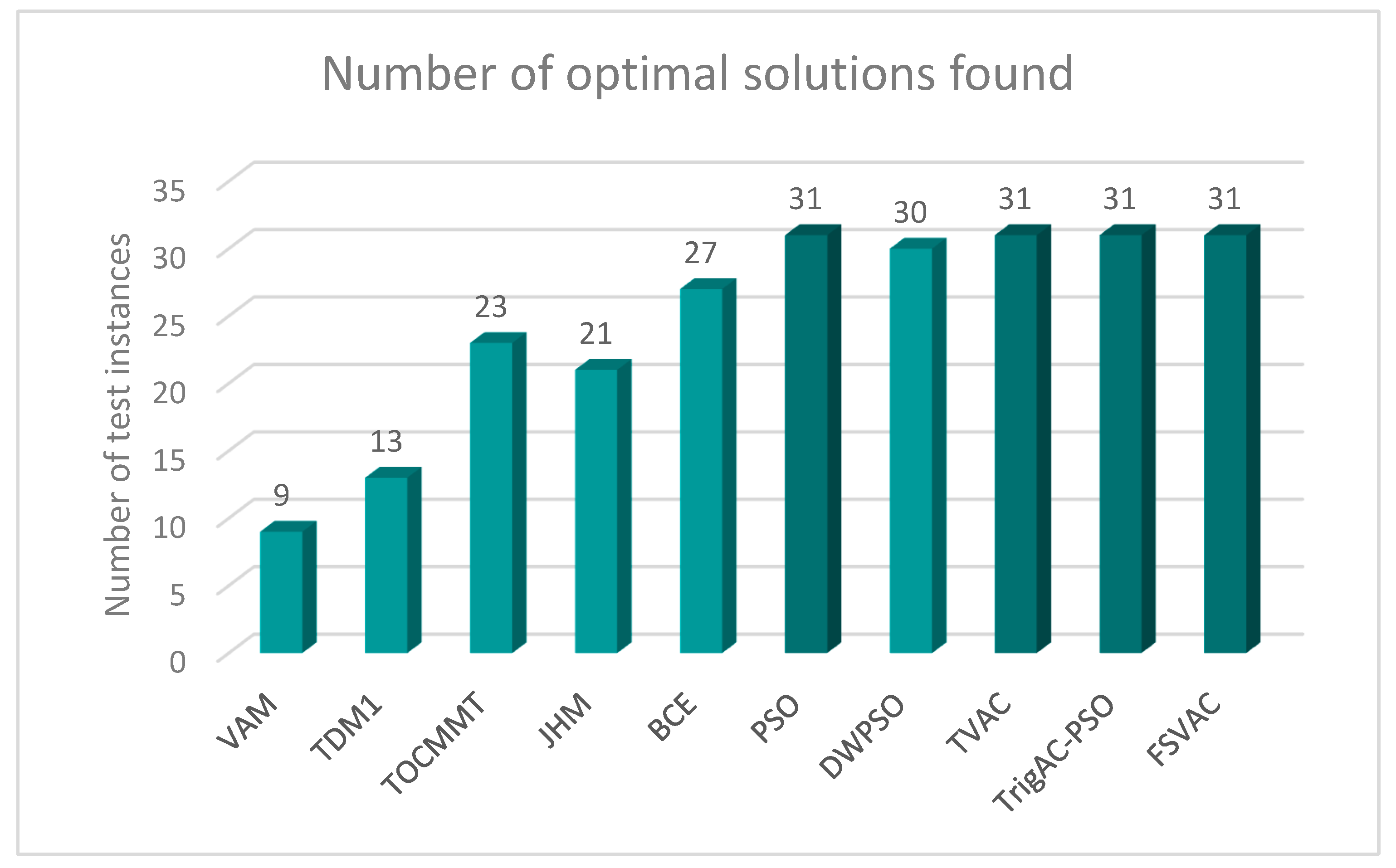
) and Figure 1, the performance of both the exact methods and the PSO-based ones are presented for 30 Monte Carlo runs; more precisely, the best value achieved by each method is depicted. The last column presents the optimal solution of each numerical problem. As shown, the Vogel method manages to find 9 out of the 32 test instances (28.13%); the Total Differences Method 1 (TDM1) succeeds in finding more optimal solutions than the Vogel method by finding 13 out of 32 optimal solutions (40.63%); using the TOCM-MT method, the results show that the method’s performance is better still, finding the optimum in 23 out of 32 test instances (71.9%); the JHM method, which accumulated 21 optimal solutions, was less effective than TOCM-MT (65.62%); the BCE method, which achieved 27 out of 32 test instances (84.4%), proved to be the most efficient compared to all previously mentioned methods; the classic PSO, the TVAC, the TrigAC-PSO and the FSVAG-PSO achieve the optimum in 31 out of 32 test instances (96.88%), while the PWPSO achieves the optimum in 30 out of the 32 (93.76%).

One significant finding of our research is that the new PSO variation, TrigAC-PSO, which is first presented in this study, achieved very good results. The following table (

Table 3. The deviation (dev) of the methods for 32 numerical examples.

	VAM	TDM1	TOCMMT	JHM	BCE	PSO	DWPSO	TVAC	TrigAC-PSO	FSVAC
Pr.01	0.085227	0	0	0	0	0	0	0	0	0
Pr.02	0.048452	0.048452	0	0	0	0	0	0	0	0
Pr.03	0	0	0	0	0	0	0	0	0	0
Pr.04	0	0	0.033898	0	0	0	0	0	0	0
Pr.05	0	0	0	0	0	0	0	0	0	0
Pr.06	0.091954	0.091954	0	0.057471	0	0	0	0	0	0
Pr.07	0	0.025641	0	0	0	0	0	0	0	0
Pr.08	0.012658	0.009494	0	0	0	0	0	0	0	0
Pr.09	0	0.081633	0.081633	0	0	0	0	0	0	0
Pr.10	0.146341	0.060976	0.060976	0.02439	0	0	0.002439	0	0	0
Pr.11	0	0	0	0	0	0	0	0	0	0
Pr.12	0.021858	0.016393	0.021858	0	0.021858	0	0	0	0	0
Pr.13	0.075094	0.075094	0	0	0	0	0	0	0	0
Pr.14	0	0	0	0	0	0.062271	0	0	0	0
Pr.15	0.051724	0	0	0.008621	0.008621	0	0	0	0	0
Pr.16	0.02	0	0	0.09	0.02	0	0	0	0	0
Pr.17	0.0333	0.0333	0	0	0	0	0	0	0	0
Pr.18	0	0	0	0	0	0	0	0	0	0
Pr.19	0	0	0	0	0.010526	0	0	0	0	0
Pr.20	0.108434	0	0	0	0	0	0	0	0	0
Pr.21	0.017341	0.031792	0	0	0	0	0	0	0	0
Pr.22	0.087912	0.087912	0	0.054945	0	0	0	0	0	0
Pr.23	0.005988	0	0	0.011976	0	0	0	0	0	0
Pr.24	0.052632	0.052632	0.052632	0.026316	0	0	0.002632	0.000439	0.001754	0.003509
Pr.25	0.211382	0.211382	0.01626	0.01626	0	0	0	0	0	0
Pr.26	0.123711	0	0	0.123711	0	0	0	0	0	0
Pr.27	0.132596	0.005525	0.154696	0	0	0	0	0	0	0
Pr.28	0.043478	0.043478	0.01087	0	0	0	0	0	0	0
Pr.29	0.061805	0.049444	0	0	0	0	0	0	0	0
Pr.30	0.141487	0.115108	0	0	0	0	0	0	0	0
Pr.31	0.092539	0.032967	0.015905	0.008386	0.008386	0	0	0	0	0
Pr.32	0.027523	0.073394	0	0.027523	0	0	0	0	0	0
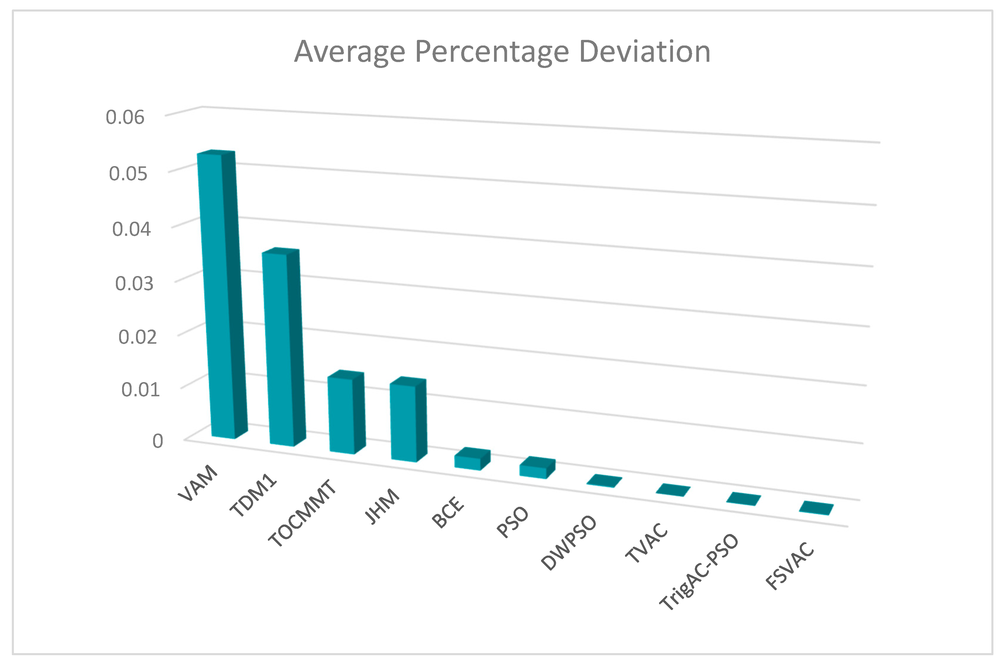
Average	0.05292	0.03583	0.014023	0.01405	0.002168	0.001946	0.000158	0.000013	0.000054	0.00011

) examines the deviation of VAM, TDM1, TOCM-MT, JHM, BCE, PSO, DuPSO, TVAC, TrigAC-PSO and FSVAC-PSO. The measurement of deviation shows the difference between the observed value and the expected value of a variable, and it is given by the following formula:

$$Dev=\frac{x_{ij}-optimal}{optimal},$$

(17)

where $x_{ij}$ is the current solution.

Considering Table 3 and Figure 2, it is evident that method VAM, TDM1, TOCM-MT and 1HM appear to be more inefficient, deviating from the optimal solution at a significant scale. More precisely, the results of Table 3 show that the solutions achieved by VAM differ from the optimal solution by 5.29%, the results of TDM1 by 3.58%, the results of TOCM-MT by 1.4% and the results of JHM by 1.4%. BCE method presented higher levels of efficiency since the values of deviation were negligible. Analysis of the data of Table 3 reveals that the percentage of the deviation in classic PSO, as well as in its variations, was almost zero. Furthermore, the TVAC method was nearest to the optimal solution, followed by TrigAC-PSO, FSVAC-PSO and finally by DWPSO.

The findings from the current study provide us with the basic information for an extensive meta-analysis, allowing us to investigate which of the presented PSO variations has better performance in solving the TP. To serve this cause, many experiments were carried out which investigated different values of PSO population size (number of particles). The classic PSO, as well as each one of its variations (DWPSO, TVAC, TrigAC-PSO, FSVAC-PSO), were tested for 10, 15 and 20 particles for all 32 numerical examples. The results presented in Table 4, Table 5 and Table 6 show the performance of the classic PSO as well of its variations for 30 independent runs. The number of generations was stable and equal to 100 for all runs.

Evidence from this study, presented in Table 4, expounds the accuracy rate of each algorithm for 10 particles. The accuracy rate is given by the following formulation:

$$Accuracy=\frac{TOR}{TR} ,$$

(18)

where $TOR$ is the total number of runs where optimal solution was found and $TR$ is the number of runs.

Table 4 shows that the classic PSO obtained 38.33% accuracy rate. A significant increase in accuracy rate, using 10 particles, was evident in DWPSO, which achieved 59.58% accuracy, almost twice as much as the percentage of the classic PSO. Moreover, TVAC obtain a 61.45% accuracy rate. The best results came from TrigAC-PSO, since this PSO variation achieved a 62.81% accuracy rate. Last but not least, FSVAC achieved a 59.5% accuracy rate.

Table 4. Accuracy of PSO, DWPSO, TVAC, TrigAC-PSO and FSVAC for 10 particles.

	PSO	DWPSO	TVAC	TrigAC-PSO	FSVAC
Pr.01	0.0333	0.2	0.4666	0.5667	0.2333
Pr.02	0.7667	1	1	1	1
Pr.03	1	1	1	1	1
Pr.04	1	1	1	1	1
Pr.05	0.2333	0.6667	0.8333	0.8667	0.8333
Pr.06	0.3667	1	0.9667	1	1
Pr.07	0.7667	0.9	1	1	0.9
Pr.08	0	0	0.2667	0.1667	0.1334
Pr.09	0.0333	0.3	0.2	0.2667	0.1
Pr.10	0	0	0.0333	0	0.0333
Pr.11	0.1	0.1	0.1333	0.1	0.0667
Pr.12	0	0.3	0.4	0.4667	0.3667
Pr.13	0.5334	1	1	0.8667	1
Pr.14	0	0	0	0.3333	0
Pr.15	0.7	1	1	1	1
Pr.16	0	0.4667	0.4667	0.6667	0.5667
Pr.17	0.4333	0.9	0.9333	0.9	0.8333
Pr.18	1	1	1	1	1
Pr.19	0.4667	0.7	0.7667	0.5	0.7333
Pr.20	0.4667	0.8333	0.6667	0.8667	0.7667
Pr.21	0.5667	0.5333	0.3333	0.5333	0.3939
Pr.22	0.3667	1	0.9667	0.8333	1
Pr.23	0.0333	0.0333	0.1667	0.1667	0.1667
Pr.24	0	0	0	0	0
Pr.25	0.5333	0.9667	0.9333	0.9667	1
Pr.26	0.4667	0.6	0.7	0.7	0.7333
Pr.27	0.0333	0.4667	0.5667	0.4	0.4667
Pr.28	0.2	0.2667	0.0667	0.2	0
Pr.29	0.8333	1	1	1	1
Pr.30	0.8667	1	1	1	1
Pr.31	0.4	0.8333	0.7	0.7	0.7
Pr.32	0.0667	0	0	0.0333	0
Average	0.383338	0.595834	0.611459	0.6281313	0.594603

Table 4. Accuracy of PSO, DWPSO, TVAC, TrigAC-PSO and FSVAC for 10 particles.

	PSO	DWPSO	TVAC	TrigAC-PSO	FSVAC
Pr.01	0.0333	0.2	0.4666	0.5667	0.2333
Pr.02	0.7667	1	1	1	1
Pr.03	1	1	1	1	1
Pr.04	1	1	1	1	1
Pr.05	0.2333	0.6667	0.8333	0.8667	0.8333
Pr.06	0.3667	1	0.9667	1	1
Pr.07	0.7667	0.9	1	1	0.9
Pr.08	0	0	0.2667	0.1667	0.1334
Pr.09	0.0333	0.3	0.2	0.2667	0.1
Pr.10	0	0	0.0333	0	0.0333
Pr.11	0.1	0.1	0.1333	0.1	0.0667
Pr.12	0	0.3	0.4	0.4667	0.3667
Pr.13	0.5334	1	1	0.8667	1
Pr.14	0	0	0	0.3333	0
Pr.15	0.7	1	1	1	1
Pr.16	0	0.4667	0.4667	0.6667	0.5667
Pr.17	0.4333	0.9	0.9333	0.9	0.8333
Pr.18	1	1	1	1	1
Pr.19	0.4667	0.7	0.7667	0.5	0.7333
Pr.20	0.4667	0.8333	0.6667	0.8667	0.7667
Pr.21	0.5667	0.5333	0.3333	0.5333	0.3939
Pr.22	0.3667	1	0.9667	0.8333	1
Pr.23	0.0333	0.0333	0.1667	0.1667	0.1667
Pr.24	0	0	0	0	0
Pr.25	0.5333	0.9667	0.9333	0.9667	1
Pr.26	0.4667	0.6	0.7	0.7	0.7333
Pr.27	0.0333	0.4667	0.5667	0.4	0.4667
Pr.28	0.2	0.2667	0.0667	0.2	0
Pr.29	0.8333	1	1	1	1
Pr.30	0.8667	1	1	1	1
Pr.31	0.4	0.8333	0.7	0.7	0.7
Pr.32	0.0667	0	0	0.0333	0
Average	0.383338	0.595834	0.611459	0.6281313	0.594603

The accuracy rate results for 15 particles are presented in Table 5. DWPSO achieved 65.31% accuracy, whereas TVAC reached 66.99%. It is of particular interest that TrigAC-PSO achieved the highest accuracy rate once again by reaching 69.8%. Finally, FSVAC obtained an accuracy rate equal to 66.56%.

Table 5. Accuracy of PSO, DWPSO, TVAC, TrigAC-PSO and FSVAC for 15 particles.

	PSO	DWPSO	TVAC	TrigAC-PSO	FSVAC
Pr.01	0.0667	0.6	0.6333	0.6333	0.4333
Pr.02	0.9667	1	1	1	1
Pr.03	1	1	1	1	1
Pr.04	1	1	1	1	1
Pr.05	0.7	0.9	1	1	1
Pr.06	0.7	1	0.9667	1	1
Pr.07	0.7667	1	1	0.9667	0.9667
Pr.08	0	0.0667	0.3333	0.1667	0.0333
Pr.09	0.0667	0.2333	0.2333	0.2	0.1333
Pr.10	0.2667	0	0	0.0667	0
Pr.11	0.2333	0.0667	0.3	0.2	0.0333
Pr.12	0.1	0.4	0.4333	0.3333	0.2
Pr.13	0.5667	1	1	0.9667	1
Pr.14	0	0.0333	0	0.0667	0.1
Pr.15	0.3	0.9333	0.9667	1	1
Pr.16	0	0.6	0.5	0.9333	0.5333
Pr.17	0.5667	0.9	1	0.9667	1
Pr.18	1	1	1	1	1
Pr.19	0.5333	0.9	0.9	0.6667	1
Pr.20	0.6334	0.9667	0.8667	0.9333	1
Pr.21	0.6667	0.4333	0.6667	1	0.4667
Pr.22	0.6	1	1	1	1
Pr.23	0.0667	0.2	0.3667	0.2333	0.2
Pr.24	0.6666	0	0	0	0
Pr.25	0.6333	1	0.8333	1	1
Pr.26	0.3333	1	0.8	0.6667	1
Pr.27	0.3667	0.4	0.4667	0.8333	1
Pr.28	0.3333	0.1333	0.1	0.3333	0.1667
Pr.29	1	1	1	1	1
Pr.30	0.9333	1	1	1	1
Pr.31	0.3667	1	0.9333	1	1
Pr.32	0.1333	0.1333	0.1	0.1667	0.0333
Average	0.486463	0.653122	0.669894	0.69791875	0.665622

Table 5. Accuracy of PSO, DWPSO, TVAC, TrigAC-PSO and FSVAC for 15 particles.

	PSO	DWPSO	TVAC	TrigAC-PSO	FSVAC
Pr.01	0.0667	0.6	0.6333	0.6333	0.4333
Pr.02	0.9667	1	1	1	1
Pr.03	1	1	1	1	1
Pr.04	1	1	1	1	1
Pr.05	0.7	0.9	1	1	1
Pr.06	0.7	1	0.9667	1	1
Pr.07	0.7667	1	1	0.9667	0.9667
Pr.08	0	0.0667	0.3333	0.1667	0.0333
Pr.09	0.0667	0.2333	0.2333	0.2	0.1333
Pr.10	0.2667	0	0	0.0667	0
Pr.11	0.2333	0.0667	0.3	0.2	0.0333
Pr.12	0.1	0.4	0.4333	0.3333	0.2
Pr.13	0.5667	1	1	0.9667	1
Pr.14	0	0.0333	0	0.0667	0.1
Pr.15	0.3	0.9333	0.9667	1	1
Pr.16	0	0.6	0.5	0.9333	0.5333
Pr.17	0.5667	0.9	1	0.9667	1
Pr.18	1	1	1	1	1
Pr.19	0.5333	0.9	0.9	0.6667	1
Pr.20	0.6334	0.9667	0.8667	0.9333	1
Pr.21	0.6667	0.4333	0.6667	1	0.4667
Pr.22	0.6	1	1	1	1
Pr.23	0.0667	0.2	0.3667	0.2333	0.2
Pr.24	0.6666	0	0	0	0
Pr.25	0.6333	1	0.8333	1	1
Pr.26	0.3333	1	0.8	0.6667	1
Pr.27	0.3667	0.4	0.4667	0.8333	1
Pr.28	0.3333	0.1333	0.1	0.3333	0.1667
Pr.29	1	1	1	1	1
Pr.30	0.9333	1	1	1	1
Pr.31	0.3667	1	0.9333	1	1
Pr.32	0.1333	0.1333	0.1	0.1667	0.0333
Average	0.486463	0.653122	0.669894	0.69791875	0.665622

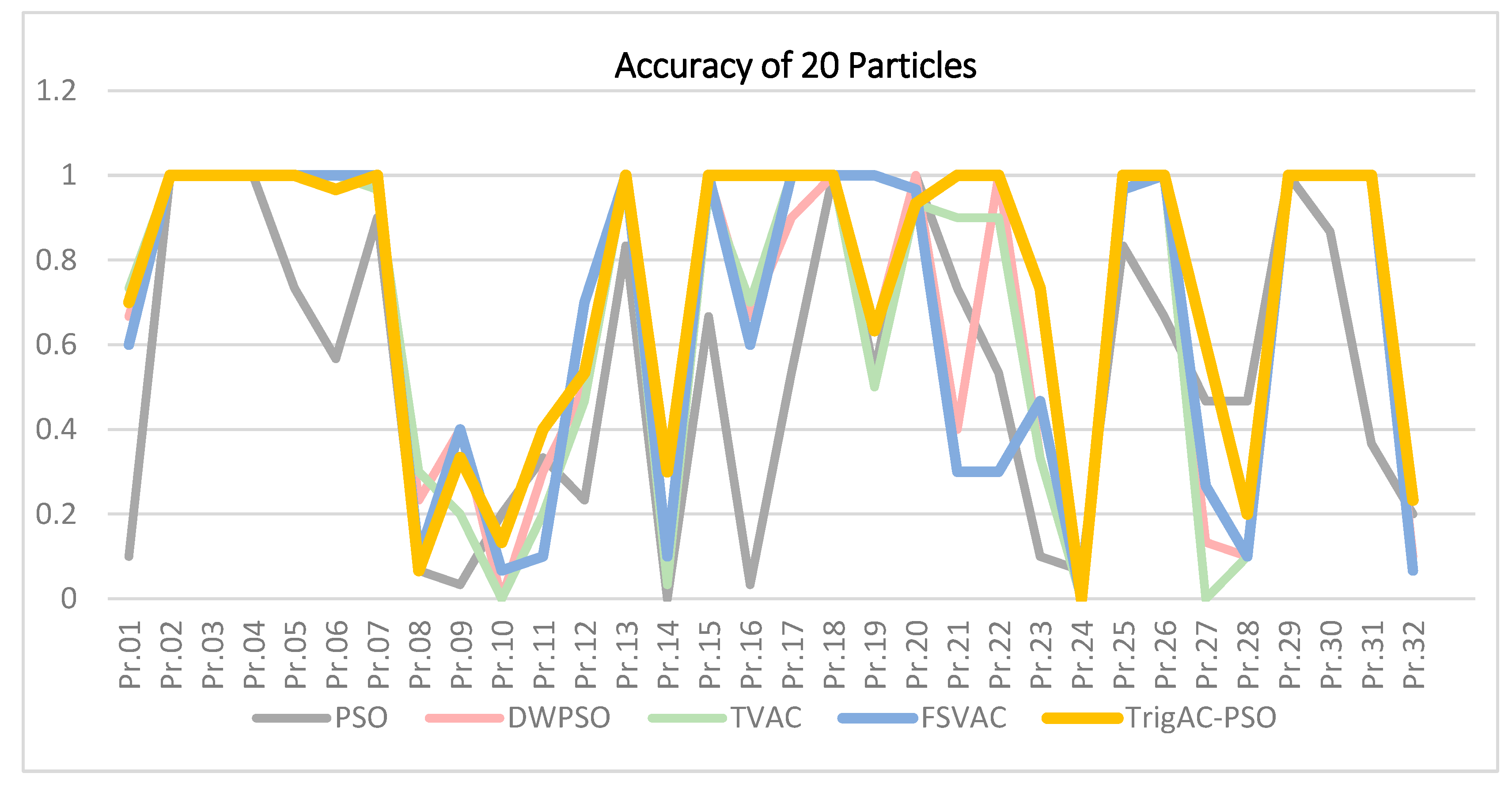
The accuracy rate results for 20 particles are presented in Table 6 and Figure 3. A high percentage of 53.33% was obtained by the classic PSO. Between DWPSO and TVAC, it is evident that both rates were sufficiently close, with accuracy rates ascending up to 66.78% and 66.56%, respectively. FSVAC, the variation which has been proposed and presented in this research, achieved accuracy rate equal to 66%. This new method evinced positive effects in terms of its validity and effectiveness. Last but not least, TrigAC-PSO demonstrated the best performance compared to all other variations, achieving 74.3%. Running the algorithm using 20 particles, TrigAC-PSO found the optimal in 31 out of 32 test instances, reaching 96.88%. Moreover, in 20 out of 32 numerical examples, this variation managed to reach the optimum in all 30 runs, with a success rate of 62.5%. The punctuality of this method rises to 75%; hence, this variation is established, compared to other variations, as the ideal option for the solution of the TP.

Table 6. Accuracy of PSO, DWPSO, TVAC, TrigAC-PSO and FSVAC for 20 particles.

	PSO	DWPSO	TVAC	TrigAC-PSO	FSVAC
Pr.01	0.1	0.6667	0.7333	0.7	0.6
Pr.02	1	1	1	1	1
Pr.03	1	1	1	1	1
Pr.04	1	1	1	1	1
Pr.05	0.7333	1	1	1	1
Pr.06	0.5667	1	1	0.9667	1
Pr.07	0.9	0.9667	0.9667	1	1
Pr.08	0.0667	0.2333	0.3	0.0667	0.1
Pr.09	0.0333	0.4	0.2	0.3333	0.4
Pr.10	0.2	0	0	0.1333	0.0667
Pr.11	0.3333	0.3	0.2	0.4	0.1
Pr.12	0.2333	0.5	0.4667	0.5333	0.7
Pr.13	0.8333	1	1	1	1
Pr.14	0	0.0333	0.0333	0.3	0.1
Pr.15	0.6667	1	0.9667	1	1
Pr.16	0.0333	0.6667	0.7	1	0.6
Pr.17	0.5333	0.9	1	1	1
Pr.18	1	1	1	1	1
Pr.19	0.5333	0.6333	0.5	0.6333	1
Pr.20	1	1	0.9333	0.9333	0.9667
Pr.21	0.7333	0.4	0.9	1	0.3
Pr.22	0.5333	1	0.9	1	0.3
Pr.23	0.1	0.3333	0.3333	0.7333	0.4667
Pr.24	0.0667	0	0	0	0
Pr.25	0.8333	1	1	1	0.9667
Pr.26	0.6667	1	1	1	1
Pr.27	0.4667	0.1333	0	0.6	0.2667
Pr.28	0.4667	0.1	0.1	0.2	0.1
Pr.29	1	1	1	1	1
Pr.30	0.8667	1	1	1	1
Pr.31	0.3667	1	1	1	1
Pr.32	0.2	0.1	0.0667	0.2333	0.0667
Average	0.533331	0.667706	0.665625	0.7427031	0.659381

Table 6. Accuracy of PSO, DWPSO, TVAC, TrigAC-PSO and FSVAC for 20 particles.

	PSO	DWPSO	TVAC	TrigAC-PSO	FSVAC
Pr.01	0.1	0.6667	0.7333	0.7	0.6
Pr.02	1	1	1	1	1
Pr.03	1	1	1	1	1
Pr.04	1	1	1	1	1
Pr.05	0.7333	1	1	1	1
Pr.06	0.5667	1	1	0.9667	1
Pr.07	0.9	0.9667	0.9667	1	1
Pr.08	0.0667	0.2333	0.3	0.0667	0.1
Pr.09	0.0333	0.4	0.2	0.3333	0.4
Pr.10	0.2	0	0	0.1333	0.0667
Pr.11	0.3333	0.3	0.2	0.4	0.1
Pr.12	0.2333	0.5	0.4667	0.5333	0.7
Pr.13	0.8333	1	1	1	1
Pr.14	0	0.0333	0.0333	0.3	0.1
Pr.15	0.6667	1	0.9667	1	1
Pr.16	0.0333	0.6667	0.7	1	0.6
Pr.17	0.5333	0.9	1	1	1
Pr.18	1	1	1	1	1
Pr.19	0.5333	0.6333	0.5	0.6333	1
Pr.20	1	1	0.9333	0.9333	0.9667
Pr.21	0.7333	0.4	0.9	1	0.3
Pr.22	0.5333	1	0.9	1	0.3
Pr.23	0.1	0.3333	0.3333	0.7333	0.4667
Pr.24	0.0667	0	0	0	0
Pr.25	0.8333	1	1	1	0.9667
Pr.26	0.6667	1	1	1	1
Pr.27	0.4667	0.1333	0	0.6	0.2667
Pr.28	0.4667	0.1	0.1	0.2	0.1
Pr.29	1	1	1	1	1
Pr.30	0.8667	1	1	1	1
Pr.31	0.3667	1	1	1	1
Pr.32	0.2	0.1	0.0667	0.2333	0.0667
Average	0.533331	0.667706	0.665625	0.7427031	0.659381

In summary, the proposed method FSVAC-PSO, although it did not demonstrate the highest average success rate, was very accurate in calculating the optimal solution in cases where the aforementioned variations were unable to approach the optimal solution. In more detail, this research experimented on population sizes of 10, 15, 20 particles over 32 well-known test instances used in the respective literature. For each problem, as already mentioned, 30 independent experimental runs were conducted. In the case of 10 particles, the classical PSO found the optimal solution in only in 3 out of 32 test instances in all 30 runs (9.4%); DWPSO found the optimal solution in 10 out of 32 test instances in all 30 runs (31.25%); while TVAC and Trig-PSO managed to find the optimal solution in 9 out of 32 test instances in all 30 runs (28.13%); finally, FSVAC was shown to be the best PSO variation, finding the optimal solution in 11 out of 32 test instances in all 30 runs (34.4%).

In the case of 15 particles, FSVAC also showed the best performance by finding in the optimal solution in 18 out of 32 test instances in all 30 runs (56.25%); the classic PSO found the optimal solution in 4 out of 32 (12.5%) test instances, and TVAC in 11 out of 32, in all 30 runs; last but not least, both DWPSO and TrigAC-PSO found the optimal value in 13 out of 32 test instances in all 30 runs (40.63%).

In the case of 20 particles, the variations TrigAC-PSO and FSVAC are still more accurate than the other PSO variations since they succeeded in finding the optimal solution in 18 out of 32 and in 17 out of 32 test instances in all 30 runs, respectively. The other PSO variations attained relatively lower success rates in finding the optimal solution in all of their runs.

In the following table (

Table 7. Statistical measures for 20 particles.

		PSO	DWPSO	TVAC	TrigAC-PSO	FSVAC
Pr.01	Mean	894.7666	884.3	883.6	882.86667	884.4
	St.Dev	22.51847	10.61278	11.2544	7.41263	8.76356
	Min	880	880	880	880	880
	Max	965	928	940	910	917
	cv%	2.51668658	1.200133	1.273701	0.8396096	0.990905
Pr.02	Mean	743	743	743	743	743
	St.Dev	0	0	0	0	0
	Min	743	743	743	743	743
	Max	743	743	743	743	743
	cv%	0	0	0	0	0
Pr.03	Mean	5600	5600	5600	5600	5600
	St.Dev	0	0	0	0	0
	Min	5600	5600	5600	5600	5600
	Max	5600	5600	5600	5600	5600
	cv%	0	0	0	0	0
Pr.04	Mean	59	59	59	59	59
	St.Dev	0	0	0	0	0
	Min	59	59	59	59	59
	Max	59	59	59	59	59
	cv%	0	0	0	0	0
Pr.05	Mean	28.266666	28	28	28	28
	St.Dev	0.4497764	0	0	0	0
	Min	28	28	28	28	28
	Max	29	28	28	28	28
	cv%	1.591190254	0	0	0	0
Pr.06	Mean	441.1333333	435	435	435	435
	St.Dev	7.619092775	0	0	0	0
	Min	435	435	435	435	435
	Max	463	435	435	435	435
	cv%	1.72716324	0	0	0	0
Pr.07	Mean	391.5	390.0333	390.4667	390	390
	St.Dev	5.015493237	0.182574	2.55603	0	0
	Min	390	390	390	390	390
	Max	410	391	404	390	390
	cv%	1.281096612	3.290831	0.654611	0	0
Pr.08	Mean	1650.933333	1593.033	1598.7	1592.1333	1629.533
	St.Dev	44.7667775	17.95873	23.31367	12.23824	40.14347
	Min	1580	1580	1580	1580	1580
	Max	1790	1642	1661	1623	1712
	cv%	2.711604194	1.127329	1.45829	0.7686698	2.463495
Pr.09	Mean	52.6	51.3	52.06667	51.6	51.16667
	St.Dev	2.40114915	2.768667	1.79910	1.90462	1.89524
	Min	49	109	49	49	49
	Max	63	122	55	53	53
	cv%	4.564922339	5.397012	3.455389	3.6911285	3.704062
Pr.10	Mean	427.4333333	427.7667	428.1	428.3	425.8
	St.Dev	8.935336025	4.38401	5.16853	6.25410	5.71386
	Min	410	411	411	410	410
	Max	434	431	431	432	430
	cv%	2.09046308	1.02486	1.20732	1.4602153	1.341913
Pr.11	Mean	2913.833333	2934.8	2864.633	2857.1	3036.767
	St.Dev	186.8538214	220.8248	226.892	11.66885	380.4261
	Min	2850	2850	2850	2850	2850
	Max	3850	3945	2977	2891	4554
	cv%	6.412646162	7.524358	1.117014	0.4084159	12.52734
Pr.12	Mean	190.5666667	184.4333	186.0333	184.33333	183.9
	St.Dev	7.623391106	1.50134	4.60496	1.49327	1.39827
	Min	183	183	183	183	183
	Max	206	186	200	186	186
	cv%	4.00038015	0.814029	2.475347	0.8100976	0.760345
Pr.13	Mean	805.3666667	799	799	799	799
	St.Dev	16.77535823	0	0	0	0
	Min	799	799	799	799	799
	Max	878	799	799	799	799
	cv%	2.082946678	0	0	0	0
Pr.14	Mean	319.9333333	302.2	290.4	290.1	292.2667
	St.Dev	21.78251962	17.70525	6.69328	16.159442	8.10250
	Min	292	273	273	273	273
	Max	378	335	317	327	306
	cv%	6.808455809	5.858785	2.304849	5.5703008	2.772298
Pr.15	Mean	1186.1	1160	1160.067	1160	1160
	St.Dev	73.12122669	0	0.36514	0	0
	Min	1160	1160	1160	1160	1160
	Max	1401	1160	1162	1160	1160
	cv%	6.164845012	0	0.031476	0	0
Pr.16	Mean	217.1333333	202.9667	202.7333	200	203.2333
	St.Dev	7.946950546	5.979755	6.53338	0	6.76034
	Min	200	200	200	200	109
	Max	237	218	220	200	119
	cv%	3.659940381	2.946176	3.222647	0	3.326397
Pr.17	Mean	244.6333333	241.6667	240	240	240
	St.Dev	6.025711195	5.195046	0	0	0
	Min	240	240	240	240	240
	Max	256	259	240	240	240
	cv%	2.463160319	2.149674	0	0	0
Pr.18	Mean	820	820	820	820	820
	St.Dev	0	0	0	0	0
	Min	820	820	820	820	820
	Max	820	820	820	820	820
	cv%	0	0	0	0	0
Pr.19	Mean	190.8	190.7	190.9333	190.56667	190
	St.Dev	0.924755326	0.952311	0.98026	0.81720	0
	Min	190	190	190	190	190
	Max	192	192	192	192	190
	cv%	0.484672603	0.499377	0.513407	0.4288264	0
Pr.20	Mean	83	83	83.3	83.2	83.1
	St.Dev	0	0	0.91538	0.761124	0.54772
	Min	83	83	83	83	83
	Max	83	83	86	86	86
	cv%	0	0	1.098902	0.914813	0.659113
Pr.21	Mean	3484.5	3536.467	3468.2	3460	3536.1
	St.Dev	58.99371679	71.42864	34.7804	0	63.5839
	Min	3460	3460	3460	3460	3460
	Max	3745	3646	3645	3460	3644
	cv%	1.693032481	2.019774	1.00284	0	1.798138
Pr.22	Mean	928.3	910	913.6	910	910
	St.Dev	28.61534433	0	14.8686	0	0
	Min	910	910	910	910	910
	Max	990	910	990	910	910
	cv%	3.08255352	0	1.627476	0	0
Pr.23	Mean	1679.1	1671.133	1670.733	1671	1671.367
	St.Dev	14.23291474	1.136642	0.58329	2.34888	2.02541
	Min	1670	1670	1670	1670	1670
	Max	1724	1675	1672	1679	1678
	cv%	0.847651405	0.068016	0.034912	0.1405674	0.121183
Pr.24	Mean	2403.966667	2366.4	2372.8	2361.5667	2333.833
	St.Dev	44.98005944	29.09627	31.0332	18.34287	117.1320
	Min	2280	2317	2320	2322	2292
	Max	2495	2430	2424	2390	2420
	cv%	1.871076669	1.229559	1.307874	0.7767247	1.47626
Pr.25	Mean	2468.766667	2460	2460	2460	2460
	St.Dev	24.21695521	0	0	0	0
	Min	2460	2460	2460	2460	2460
	Max	2563	2460	2460	2460	2460
	cv%	0.980933335	0	0	0	0
Pr.26	Mean	292.6	291	291	291	291
	St.Dev	2.485821865	0	0	0	0
	Min	291	291	291	291	291
	Max	299	291	291	291	291
	cv%	0.84956318	0	0	0	0
Pr.27	Mean	4574.233333	4639.967	4666.433	4535	4634.9
	St.Dev	73.42821187	60.22915	29.96973	18.34910	67.4073
	Min	4525	4525	4529	4525	4525
	Max	4753	4675	4677	4585	4675
	cv%	1.605257243	1.298051	0.642241	0.4046109	1.454343
Pr.28	Mean	941.7	953.3667	953.0667	947.26667	947.9667
	St.Dev	22.49314072	19.67404	13.35957	17.26454	13.60396
	Min	920	920	920	920	920
	Max	974	992	960	960	968
	cv%	2.38856756	2.063638	1.401746	1.8225639	1.435068
Pr.29	Mean	809	809	809	809	809
	St.Dev	0	0	0	0	0
	Min	809	809	809	809	809
	Max	809	809	809	809	809
	cv%	0	0	0	0	0
Pr.30	Mean	419.5333333	417	417	417	417
	St.Dev	7.103827688	0	0	0	0
	Min	417	417	417	417	417
	Max	445	417	417	417	417
	cv%	1.693268955	0	0	0	0
Pr.31	Mean	3480.066667	3458	3458	3458	3458
	St.Dev	33.27620392	0	0	0	0
	Min	3458	3458	3458	3458	3458
	Max	3587	3458	3458	3458	3458
	cv%	0.956194438	0	0	0	0
Pr.32	Mean	114.3	116.9333	114.4333	114.7	118.4333
	St.Dev	3.761419395	4.532894	3.549485	3.77057	4.44648
	Min	109	109	109	109	109
	Max	122	125	127	119	125
	cv%	3.290830616	3.876477	3.101794	3.2873372	3.754424

), the most important statistical measures in the cases of 20 particles for 30 independent runs are represented for all PSO variations. These experimental results demonstrate the very good performance and stability of the proposed PSO variations in solving the TP. As presented, in all cases, the mean value is very close to the best one, showing that all these variations are not only efficient but also quite stable. The value of the Coefficient of Variation (CV), which is the basic measure for proving stability of stochastic algorithms, is, for all PSO variations, quite small; more precisely, the mean CV value is for each PSO variation is as follows: Classic PSO, 2.12%; DWPSO, 1.32%; TVAC, 0.87%; TrigAC-PSO, 0.66%; and FSVAC, 1.26%. These values show that TrigAC-PSO, which is one of the new PSO variations presented in this work, is the most stable one.

The above results urged us to continue the research for an even greater number of particles, in order to study the behavior of new variations in a multi-solution environment.

More specifically, the aforementioned variations were also tested on the set of 40 and 50 particles. In this case, 10 independent runs were carried out for each test instance, reducing the chances of finding the optimal solution from the 30 independent runs that we have already performed. Selecting more particles revealed significant results.

The results showed, once again, the consistent superiority of the proposed variations.

Table 8. Accuracy of PSO, DWPSO, TVAC, TrigAC-PSO and FSVAC for 40 particles.

	PSO	DWPSO	TVAC	TrigAC-PSO	FSVAC
Pr.01	0.2	0.8	0.8	1	0.8
Pr.02	1	1	1	1	1
Pr.03	1	1	1	1	1
Pr.04	1	1	1	1	1
Pr.05	1	1	1	1	1
Pr.06	0.4	1	1	1	1
Pr.07	0.8	1	1	1	1
Pr.08	0.2	0.2	0.3	0.7	0.1
Pr.09	0	0.5	0.3	0.6	0.3
Pr.10	0.2	0.5	0.2	0.5	0.6
Pr.11	0	0.5	0.4	0.8	0.4
Pr.12	0.2	0.7	0.7	0.7	1
Pr.13	0.7	1	1	1	1
Pr.14	0	0.3	0.5	0.7	0.5
Pr.15	0.8	1	1	1	1
Pr.16	0.2	1	0.8	1	1
Pr.17	0.3	1	1	1	1
Pr.18	1	1	1	1	1
Pr.19	0.2	0.9	0.6	0.9	1
Pr.20	1	0.9	1	1	1
Pr.21	0.6	0.5	0.6	0.7	0.4
Pr.22	0.7	1	1	1	1
Pr.23	0.1	0.7	0.9	1	0.8
Pr.24	0	0	0	0	0
Pr.25	0.7	1	1	1	1
Pr.26	0.8	1	1	1	1
Pr.27	0.8	0.5	0.2	0.9	0.6
Pr.28	0	0.1	0.4	0.6	0.3
Pr.29	1	1	1	1	1
Pr.30	1	1	1	1	1
Pr.31	0.5	1	1	1	1
Pr.32	0.1	0.2	0.1	0.2	0
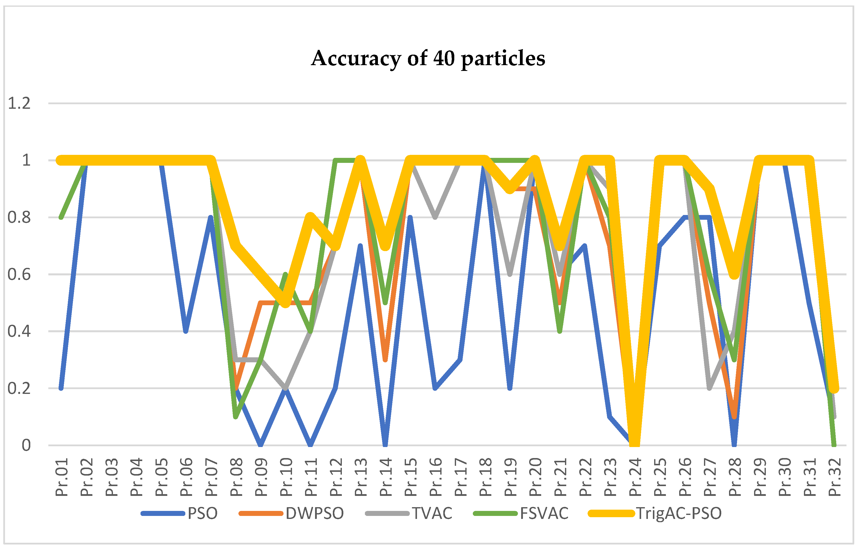
Average	0.515625	0.759375	0.74375	0.853125	0.775

and Figure 4 shows the accuracy achieved by each variation for 40 particles. These results provide further support for the hypothesis that TrigAC-PSO and FSVAC are still more accurate than the other PSO variations, since they attained accuracy rates 88.31% and 77.5%, respectively; the DWPSO method follows with 75.94%, and TVAC with 74.38%; last but not least is the classic PSO with 51.56%, attaining a spectacular 13% increase over the 10-particle accuracy rates, but maintaining a steady performance for 15 and 20 particles.

In the following table (

Table 9. Statistical measures for 40 particles.

		PSO	DWPSO	TVAC	TrigAC-PSO	FSVAC
Pr.01	Mean	900.6	882.6	879.6	880	886.5
	Var	32.69455	7.229569	2.065591	0	13.94633
	Min	880	880	874	880	880
	Max	975	903	882	880	918
	cv%	3.630307	0.819122	0.234833	0	1.57319
Pr.02	Mean	743	743	743	743	743
	Var	0	0	0	0	0
	Min	743	743	743	743	743
	Max	743	743	743	743	743
	cv%	0	0	0	0	0
Pr.03	Mean	5600	5600	5600	5600	5600
	Var	0	0	0	0	0
	Min	5600	5600	5600	5600	5600
	Max	5600	5600	5600	5600	5600
	cv%	0	0	0	0	0
Pr.04	Mean	59	59	59	59	59
	Var	0	0	0	0	0
	Min	59	59	59	59	59
	Max	59	59	59	59	59
	cv%	0	0	0	0	0
Pr.05	Mean	28	28	28	28	28
	Var	0	0	0	0	0
	Min	28	28	28	28	28
	Max	28	28	28	28	28
	cv%	0	0	0	0	0
Pr.06	Mean	443.2	435	435	435	435
	Var	11.51617	0	0	0	0
	Min	435	435	435	435	435
	Max	472	435	435	435	435
	cv%	2.598414	0	0	0	0
Pr.07	Mean	393.9	390	390	390	390
	Var	8.2253	0	0	0	0
	Min	390	390	390	390	390
	Max	410	390	390	390	390
	cv%	2.08817	0	0	0	0
Pr.08	Mean	1659.4	1595.4	1611.5	1586.3	1623.8
	Var	74.99363	23.41035	53.60193	18.53555	32.25179
	Min	1580	1580	1571	1580	1580
	Max	1802	1650	1717	1639	1671
	cv%	4.519322	1.467365	3.326213	1.168477	1.986192
Pr.09	Mean	52.4	50.2	50.5	49.7	50.4
	Var	1.577621	1.619328	1.509231	1.251666	1.074968
	Min	50	49	49	49	49
	Max	55	53	53	53	52
	cv%	3.010728	3.225752	2.988576	2.518442	2.132872
Pr.10	Mean	421.7	417	417.2	414.3	414.7
	Var	11.72888	9.092121	6.924995	5.945119	6.848357
	Min	410	410	410	410	410
	Max	434	430	430	425	430
	cv%	2.781333	2.180365	1.659874	1.434979	1.6514
Pr.11	Mean	3273.9	2894	2852.8	2850.2	3016.8
	Var	557.6408	121.5237	4.391912	0.421637	255.7915
	Min	2851	2850	2850	2850	2850
	Max	4360	3237	2864	2851	3513
	cv%	17.03292	4.199159	0.153951	0.014793	8.478901
Pr.12	Mean	190.9	185.2	183.7	183.9	183
	Var	7.218033	4.289522	1.251666	1.449138	0
	Min	183	183	183	183	183
	Max	203	196	186	186	183
	cv%	3.781054	2.316157	0.681364	0.788003	0
Pr.13	Mean	807.4	799	799	799	799
	Var	13.52528	0	0	0	0
	Min	799	799	799	799	799
	Max	827	799	799	799	799
	cv%	1.675165	0	0	0	0
Pr.14	Mean	300.9	284.6	280	276.9	281.8
	Var	15.16905	10.25454	8.628119	6.707376	9.29516
	Min	290	273	273	273	273
	Max	330	302	290	291	292
	cv%	5.041225	3.603141	3.081471	2.42231	3.298495
Pr.15	Mean	1160.4	1160	1160	1160	1160
	Var	0.843274	0	0	0	0
	Min	1160	1160	1160	1160	1160
	Max	1162	1160	1160	1160	1160
	cv%	0.072671	0	0	0	0
Pr.16	Mean	215.2	200	201.6	200	200
	Var	8.243516	0	4.718757	0	0
	Min	200	200	200	200	200
	Max	221	200	215	200	200
	cv%	3.83063	0	2.340653	0	0
Pr.17	Mean	244.7	240	240	240	240
	Var	6.236986	0	0	0	0
	Min	240	240	240	240	240
	Max	256	240	240	240	240
	cv%	2.54883	0	0	0	0
Pr.18	Mean	820	820	820	820	820
	Var	0	0	0	0	0
	Min	820	820	820	820	820
	Max	820	820	820	820	820
	cv%	0	0	0	0	0
Pr.19	Mean	191.4	190.2	190.7	190.1	190
	Var	0.843274	0.632456	0.948683	0.316228	0
	Min	190	190	190	190	190
	Max	192	192	192	191	190
	cv%	0.440582	0.332521	0.497474	0.166348	0
Pr.20	Mean	83.3	83.3	83	83	83
	Var	0.948683	0.948683	0	0	0
	Min	83	83	83	83	83
	Max	86	86	83	83	83
	cv%	1.138876	1.138876	0	0	0
Pr.21	Mean	3529.4	3482.4	3479.3	3469.3	3482
	Var	136.2777	28.33608	40.89567	16.54657	28.15828
	Min	3460	3460	3460	3460	3460
	Max	3805	3545	3590	3502	3544
	cv%	3.861213	0.813694	1.175399	0.476943	0.808681
Pr.22	Mean	919.6	910	910	910	910
	Var	16.46005	0	0	0	0
	Min	910	910	910	910	910
	Max	954	910	910	910	910
	cv%	1.789914	0	0	0	0
Pr.23	Mean	1674.4	1670.3	1670.1	1670	1671
	Var	4.718757	0.483046	0.316228	0	2.538591
	Min	1670	1670	1670	1670	1670
	Max	1686	1671	1671	1670	1678
	cv%	0.281818	0.02892	0.018935	0	0.15192
Pr.24	Mean	2412.6	2370	2352.5	2349	2351.1
	Var	20.74823	19.47648	34.42302	21.34895	29.51252
	Min	2371	2341	2287	2315	2296
	Max	2441	2397	2419	2393	2394
	cv%	0.859994	0.821792	1.463253	0.908853	1.255264
Pr.25	Mean	2479	2460	2460	2460	2460
	Var	31.34042	0	0	0	0
	Min	2460	2460	2460	2460	2460
	Max	2540	2460	2460	2460	2460
	cv%	1.264237	0	0	0	0
Pr.26	Mean	292.2	291	291	291	291
	Var	2.699794	0	0	0	0
	Min	291	291	291	291	291
	Max	299	291	291	291	291
	cv%	0.923954	0	0	0	0
Pr.27	Mean	4550.9	4538.4	4578.5	4525.6	4556.4
	Var	54.61471	20.28245	59.81871	1.897367	62.54634
	Min	4525	4525	4525	4525	4525
	Max	4657	4585	4675	4531	4675
	cv%	1.200086	0.446908	1.306513	0.041925	1.372714
Pr.28	Mean	971.9	931	934.1	924.7	930.3
	Var	11.97637	14.96663	15.05139	8.525126	12.5614
	Min	960	920	920	920	920
	Max	993	969	955	947	960
	cv%	1.232263	1.607586	1.611326	0.921934	1.350253
Pr.29	Mean	809	809	809	809	809
	Var	0	0	0	0	0
	Min	809	809	809	809	809
	Max	809	809	809	809	809
	cv%	0	0	0	0	0
Pr.30	Mean	417	417	417	417	417
	Var	0	0	0	0	0
	Min	417	417	417	417	417
	Max	417	417	417	417	417
	cv%	0	0	0	0	0
Pr.31	Mean	3469.5	3458	3458	3458	3458
	Var	12.40296	0	0	0	0
	Min	3458	3458	3458	3458	3458
	Max	3483	3458	3458	3458	3458
	cv%	0.357485	0	0	0	0
Pr.32	Mean	115	118.6	121.4	115	117.1
	Var	2.94392	8.126773	8.448537	4.944132	2.330951
	Min	109	109	109	109	112
	Max	119	129	129	123	120
	cv%	2.559931	6.852254	6.959256	4.299245	1.990565

), the most important statistical measures in the case of 40 particles for 10 independent runs are represented for all PSO variations. According to the particularly low values of the Coefficient of Variation (CV), we can infer that the PSO variations are extremely stable; more precisely, the mean CV value for each PSO variation is as follows: Classic PSO, 2.14%; DWPSO, 0.93%; TVAC, 0.86%; TrigAC-PSO, 0.47%; and FSVAC, 0.81%. These values show that TrigAC-PSO, which is one of the new PSO variations presented in this work, is once again the most stable method.

The following table (

Table 10. Accuracy of PSO, DWPSO, TVAC, TrigAC-PSO and FSVAC for 50 particles.

	PSO	DWPSO	TVAC	TrigAC-PSO	FSVAC
Pr.01	0.2	1	1	1	1
Pr.02	1	1	1	1	1
Pr.03	1	1	1	1	1
Pr.04	1	1	1	1	1
Pr.05	1	1	1	1	1
Pr.06	0.7	1	1	1	1
Pr.07	0.9	1	1	1	1
Pr.08	0.2	0.3	0.3	0.4	0.1
Pr.09	0	0.6	0.5	0.8	0.5
Pr.10	0.1	0.1	0.4	0.7	0.5
Pr.11	0.3	0.4	0.6	1	0.5
Pr.12	0.2	0.7	0.5	0.8	1
Pr.13	0.8	1	1	1	1
Pr.14	0	0.3	0.2	0.7	1
Pr.15	0.8	1	1	1	1
Pr.16	0.1	1	1	1	1
Pr.17	0.3	0.7	1	1	1
Pr.18	1	1	1	1	1
Pr.19	0.2	0.9	0.8	0.9	1
Pr.20	0.7	1	1	1	1
Pr.21	0.5	0.3	0.6	1	0.4
Pr.22	0.8	1	1	1	1
Pr.23	0.2	0.8	0.6	1	0.8
Pr.24	0	0	0.1	0	0
Pr.25	1	1	1	1	1
Pr.26	0.7	1	1	1	1
Pr.27	0.5	0.3	0.1	0.6	0.5
Pr.28	0.1	0.4	0.7	0.7	0.7
Pr.29	1	1	1	1	1
Pr.30	1	1	1	1	1
Pr.31	0.5	1	1	1	1
Pr.32	0	0	0.1	0.2	0.3
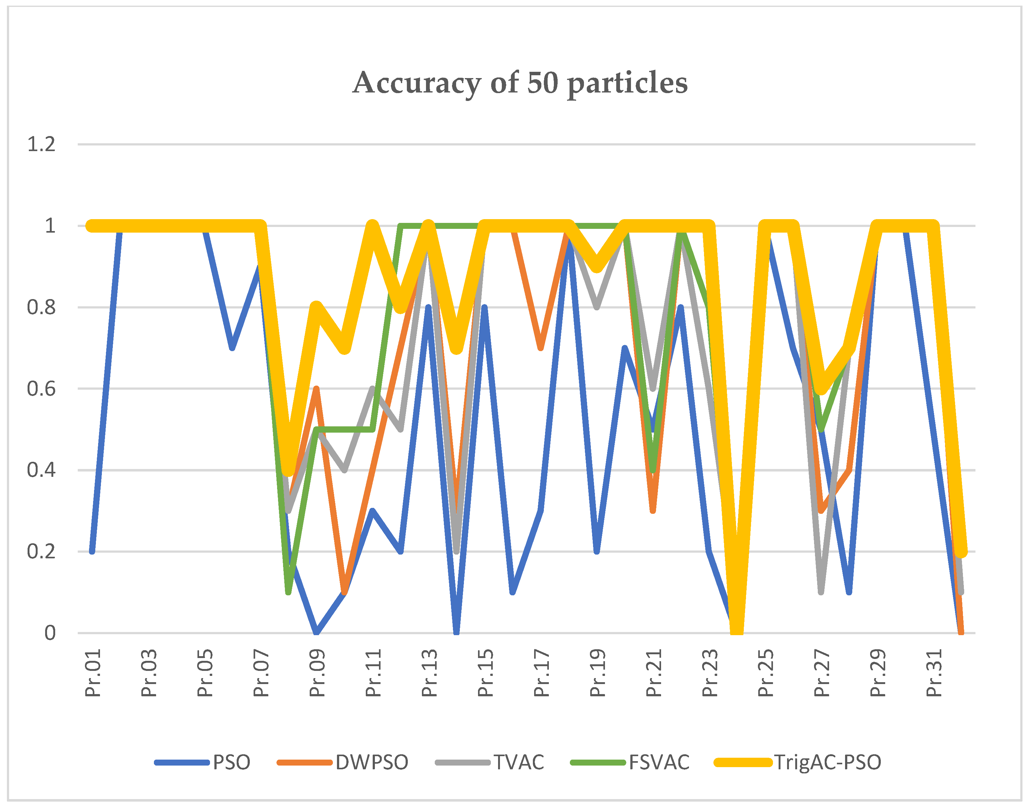
Average	0.525	0.74375	0.765625	0.86875	0.821875

) and Figure 5 present the accuracy for the 50 particles. The accuracy for each PSO variation is as follows: Classic PSO, 52.5%; DWPSO, 74.3%; TVAC, 76.56%; TrigAC-PSO, 86.88%; and FSVAC, 82.19%. The two new variations range at the highest levels. These are particularly promising results, demonstrating that the increase in the particle’s number leads to an increase in the PSO variation’s accuracy, especially in the case of TrigAC-PSO and FSVAC. The results of 50 particles are equal to or better than the results that are currently presented. Overall, TrigAC-PSO was the one that obtained the most robust results.

The results of

Table 11. Statistical measures for 50 particles.

		PSO	DWPSO	TVAC	TrigAC-PSO	FSVAC
	Mean	896.7	880	880	880	880
	Var	17.79544	0	0	0	0
Pr.01	Min	880	880	880	880	880
	Max	929	880	880	880	880
	cv%	1.984548	0	0	0	0
	Mean	743	743	743	743	743
	Var	0	0	0	0	0
Pr.02	Min	743	743	743	743	743
	Max	743	743	743	743	743
	cv%	0	0	0	0	0
	Mean	5600	5600	5600	5600	5600
	Var	0	0	0	0	0
Pr.03	Min	5600	5600	5600	5600	5600
	Max	5600	5600	5600	5600	5600
	cv%	0	0	0	0	0
	Mean	59	59	59	59	59
	Var	0	0	0	0	0
Pr.04	Min	59	59	59	59	59
	Max	59	59	59	59	59
	cv%	0	0	0	0	0
	Mean	28	28	28	28	28
	Var	0	0	0	0	0
Pr.05	Min	28	28	28	28	28
	Max	28	28	28	28	28
	cv%	0	0	0	0	0
	Mean	438.9	435	435	435	435
	Var	6.279597	0	0	0	0
Pr.06	Min	435	435	435	435	435
	Max	448	435	435	435	435
	cv%	1.430758	0	0	0	0
	Mean	392	390	390	390	390
	Var	6.324555	0	0	0	0
Pr.07	Min	390	390	390	390	390
	Max	410	390	390	390	390
	cv%	1.613407	0	0	0	0
	Mean	1677.3	1611.7	1601.7	1585.9	1634.5
	Var	73.73986	47.30058	31.18778	7.125073	41.31518
Pr.08	Min	1580	1580	1580	1580	1580
	Max	1794	1713	1672	1595	1705
	cv%	4.396343	2.934825	1.947168	0.449276	2.527696
	Mean	52.4	50.3	50.2	49.4	50.8
	Var	0.966092	1.888562	1.549193	0.843274	2.043961
Pr.09	Min	51	49	49	49	49
	Max	53	53	53	51	54
	cv%	1.843687	3.754597	3.086043	1.707032	4.023546
	Mean	424.1	421	418.6	412.6	416.1
	Var	9.362455	8.589399	9.057839	4.299871	8.292567
Pr.10	Min	410	410	410	410	410
	Max	432	430	430	421	430
	cv%	2.207605	2.040237	2.163841	1.04214	1.992926
	Mean	3149.1	2870.4	2856.9	2850	2898.3
	Var	611.9779	44.53014	14.0115	0	95.44405
Pr.11	Min	2850	2850	2850	2850	2850
	Max	4429	2990	2894	2850	3091
	cv%	19.43342	1.551357	0.490444	0	3.293105
	Mean	187.4	183.9	184.5	183.6	183
	Var	3.687818	1.449138	1.581139	1.264911	0
Pr.12	Min	183	183	183	183	183
	Max	193	186	186	186	183
	cv%	1.967886	0.788003	0.856986	0.688949	0
	Mean	804.6	799	799	799	799
	Var	11.80584	0	0	0	0
Pr.13	Min	799	799	799	799	799
	Max	827	799	799	799	799
	cv%	1.467293	0	0	0	0
	Mean	302.8	284.2	289.2	278.1	273
	Var	15.38975	7.871185	15.59772	8.491172	0
Pr.14	Min	290	273	273	273	273
	Max	328	291	328	295	273
	cv%	5.082481	2.769594	5.393403	3.05328	0
	Mean	1184.3	1160	1160	1160	1160
	Var	76.14321	0	0	0	0
Pr.15	Min	1160	1160	1160	1160	1160
	Max	1401	1160	1160	1160	1160
	cv%	6.429386	0	0	0	0
	Mean	212.9	200	200	200	200
	Var	8.69802	0	0	0	0
Pr.16	Min	200	200	200	200	200
	Max	221	200	200	200	200
	cv%	4.085496	0	0	0	0
	Mean	246.9	241.6	240	240	240
	Var	6.773314	2.796824	0	0	0
Pr.17	Min	240	240	240	240	240
	Max	256	248	240	240	240
	cv%	2.743343	1.157626	0	0	0
	Mean	820	820	820	820	820
	Var	0	0	0	0	0
Pr.18	Min	820	820	820	820	820
	Max	820	820	820	820	820
	cv%	0	0	0	0	0
	Mean	191.6	190.1	190.3	190.1	190
	Var	0.843274	0.316228	0.674949	0.316228	0
Pr.19	Min	190	190	190	190	190
	Max	192	191	192	191	190
	cv%	0.440122	0.166348	0.354676	0.166348	0
	Mean	83.9	83	83	83	83
	Var	1.449138	0	0	0	0
Pr.20	Min	83	83	83	83	83
	Max	86	83	83	83	83
	cv%	1.72722	0	0	0	0
	Mean	3493.6	3468.4	3477.6	3460	3470.8
	Var	57.87765	13.1673	24.84262	0	12.76105
Pr.21	Min	3460	3456	3460	3460	3460
	Max	3625	3492	3519	3460	3495
	cv%	1.656676	0.379636	0.714361	0	0.367669
	Mean	914.7	910	910	910	910
	Var	10.133	0	0	0	0
Pr.22	Min	910	910	910	910	910
	Max	938	910	910	910	910
	cv%	1.107795	0	0	0	0
	Mean	1675.2	1670.2	1672	1670	1670.6
	Var	7.743097	0.421637	3.018462	0	1.577621
Pr.23	Min	1670	1670	1670	1670	1670
	Max	1694	1671	1679	1670	1675
	cv%	0.462219	0.025245	0.18053	0	0.094434
	Mean	2423.4	2354.5	2336.8	2347	2355
	Var	13.35165	31.64824	37.90573	26.48689	28.5151
Pr.24	Min	2401	2288	2280	2307	2309
	Max	2446	2390	2404	2388	2395
	cv%	0.550947	1.34416	1.622121	1.128543	1.210832
	Mean	2460	2460	2460	2460	2460
	Var	0	0	0	0	0
Pr.25	Min	2460	2460	2460	2460	2460
	Max	2460	2460	2460	2460	2460
	cv%	0	0	0	0	0
	Mean	292.2	291	291	291	291
	Var	1.932184	0	0	0	0
Pr.26	Min	291	291	291	291	291
	Max	295	291	291	291	291
	cv%	0.661254	0	0	0	0
	Mean	4585.8	4549.3	4552.3	4532	4595.2
	Var	69.97904	45.93486	42.05829	16.57307	75.36843
Pr.27	Min	4525	4525	4525	4525	4525
	Max	4675	4675	4668	4577	4675
	cv%	1.525994	1.009713	0.923891	0.36569	1.640156
	Mean	957.3	928	929.9	923.3	923.6
	Var	21.12424	12.26558	17.85404	8.420214	9.070097
Pr.28	Min	920	920	920	920	920
	Max	990	960	967	947	949
	cv%	2.206647	1.321722	1.919995	0.911969	0.982037
	Mean	809	809	809	809	809
	Var	0	0	0	0	0
Pr.29	Min	809	809	809	809	809
	Max	809	809	809	809	809
	cv%	0	0	0	0	0
	Mean	417	417	417	417	417
	Var	0	0	0	0	0
Pr.30	Min	417	417	417	417	417
	Max	417	417	417	417	417
	cv%	0	0	0	0	0
	Mean	3470.4	3458	3458	3458	3458
	Var	18.42221	0	0	0	0
Pr.31	Min	3458	3458	3458	3458	3458
	Max	3508	3458	3458	3458	3458
	cv%	0.530838	0	0	0	0
	Mean	118.1	122.3	123.7	114.1	112.6
	Var	5.384133	6.498718	8.590046	3.784471	3.306559
Pr.32	Min	112	11a2	109	109	109
	Max	127	129	129	120	119
	cv%	4.558961	5.313751	6.944257	3.316802	2.936553

lead to similar conclusions. In order to examine the stability for the 50 particles, it is worth comparing the CV values of the proposed variations with those of the traditional variations. Superior results are seen from TrigAC-PSO, as the CV value is equal to 0.4%, followed by the FSVAC with 0.59%. The other values of variations ranged as follows: Classic PSO, 2.19%; DWPSO, 0.77%; and TVAC, 0.83%.

The overall results demonstrate two inferences of decisive importance: first, the PSO algorithm and its variations have successfully solved the TP with maximum accuracy and efficiency; second, TrigAC-PSO, beyond any doubt, is the leading option for solving the TP in terms of both stability and the solution’s quality.

7. Conclusions

As technology is developing, the need for product improvement and trading is of high priority in obtaining a more economical solution. The PSO algorithm was applied with success in order for the TP to be solved. Furthermore, two new variations were introduced and compared to already-known variations. These variations induced exceptional results and indicated their superiority against the existing variations and the well-known exact methods in the literature. The proposed PSO variations have been tested in a variety of test instances with different combined values of inertia weight as well as social and personal acceleration parameters. It was evidently proven that the solution quality is inseparably linked with the selection of proper values for controlling the algorithm parameters. In order to see the effectiveness and stability of the proposed variations, we compared their results with those of other PSO variations for the same instances. Remarkably, the punctuality of one of our variations rose to 88%, and it was finally established as the ideal option compared to all other variations for the solution of TP.

It can be easily observed that this PSO variationis simple compared to other variations with complex structures. It was a challenge to achieve better results by creating and running simple computational algorithms, proving that keeping a balance between human and artificial intelligence is the key to the success of computational intelligence.

A more comprehensive analysis may be needed in order to examine the TP to a greater extent. Moreover, the proposed PSO variations could be applied to more complex networks such as the Sioux Fall network [27] in order to demonstrate the algorithm’s good performance and independence of the network’s size. Except for this, some other real constraints can be proposed in order to find the optimal solution for the TP with PSO algorithm variations not only in balanced instances but also in more realistic unbalanced instances in the future. Moreover, combining the proposed PSO variations with other meta-heuristic methods to solve the TP will be an interesting challenge.