An Algorithm for the Fisher Information Matrix of a VARMAX Process

Abstract

In this paper, an algorithm for Mathematica is proposed for the computation of the asymptotic Fisher information matrix for a multivariate time series, more precisely for a controlled vector autoregressive moving average stationary process, or VARMAX process. Meanwhile, we present briefly several algorithms published in the literature and discuss the sufficient condition of invertibility of that matrix based on the eigenvalues of the process operators. The results are illustrated by numerical computations.

1. Introduction

In this paper, we present an algorithm for the symbolic software package Mathematica to compute the asymptotic Fisher information matrix for a multivariate time series, more precisely a controlled vector autoregressive moving average stationary process, or VARMAX process. There are several ways to obtain the Fisher information matrix for time series models. The most used procedure is computing the Hessian of the Gaussian log-likelihood when a model is fitted to the time series, usually after non-linear optimization (since the model is non-linear with respect to the parameters except for the pure VAR case), e.g., [1]. Another much less used method consists of determining the exact (Gaussian) Fisher information, see [2,3,4,5,6,7,8]. This is nice when the data are available but, as [9] indicates, it can be useful to know the matrix at a tentative parameter point before obtaining the data, in order to determine the series length necessary to reach some specific accuracy for the estimators of the parameters. Then, an algorithm for the computation of the so-called asymptotic Fisher information matrix at a given parameter point is what is needed. It was provided in the form of an algebraic expression for a handful of small-order (1 or 2) ARMA models by Box and Jenkins in 1970, see [10]. Otherwise, there is a vast literature for scalar models, i.e., simple ARMA models, e.g., [11,12], seasonal ARMA models [13], ARMAX models [14], single input single output models [15], and for vector models, i.e., VARMA models [16,17] and VARMAX models [18,19].

We introduce a new algorithm well-suited to symbolic computation software packages (here Mathematica) and we present an illustrative example. Then, we discuss the invertibility of the Fisher information matrices and provide other examples.

The proposed algorithm differs from the works of Zadrovny [3,20], see also Zadrozny and Mittnick [21], who developed their methods for VARMAX models, in the sense that they are based on an approximation of the exact Fisher information. Here, we follow Whittle’s approach [22] of expressing the asymptotic information matrix by computing a circular integral of a rational function, related to the autoregressive and moving average operators. That was the way used by Newton for VARMA models, see [16], with the difference that we make the effective computation and that we consider VARMAX models. The more fundamental source is [19], who obtained an explicit expression for the Fisher information matrix of a VARMAX model under the form of a sum of two integrals while [18] contains expressions for each element of that matrix. As a matter of fact, we first need to generalize [19], which is developed for the special case where the number of explanatory variables equals the number of variables of interest and, moreover, the coefficient matrix at lag 0 is the identity matrix. These restrictions were explained by the revealed objective of the paper which was to exploit tensor Sylvester matrices and try to extend to VARMAX models the resultant property of the Fisher information matrix wrongly claimed for VARMA models by [17]. Indeed, in [17] (p. 1986), it is written “[a] representation [based on tensor Sylvester matrices] is more appropriate …to prove a possible resultant property of the Fisher information matrix of a VARMAX process”. Such a tensor Sylvester matrix is associated with two matrix polynomials and it becomes singular if, and only if, the two matrix polynomials have at least one common eigenvalue, see [23].

In [17], it is said that the Fisher information matrix of a VARMA process becomes invertible if, and only if, the tensor Sylvester matrix is invertible, in other words, if, and only if, the autoregressive and moving average matrix polynomials of the VARMA process have no common eigenvalue. This is called the Sylvester resultant property. In [17], the Sylvester resultant property is shown for a scalar ARMAX process but it is no longer true, in general, for other than scalar ARMA or ARMAX processes. Indeed, in [24] Mélard indicated the error in the claim and explained why the example in [17] was wrong. In the present paper, we correct the assertion stated in [17] for VARMA processes, and we extend the “if” part to a class of VARMAX processes. As will be shown, the “only if” part of that result is, however, wrong when the dimension of the process is larger than 1. We will also compare our algorithms with other algorithms proposed for special cases in the literature. Although the results are less powerful, they are what is needed in practice: a sufficient condition of invertibility of the Fisher information matrix, indicating a possible lack of identifiability so that parameter estimation is risky. A necessary condition that should involve more information about the matrix polynomials is not as useful.

Consider the vector stochastic difference equation representation of a linear system of order $(p,r,q)$ of the process $\{y_t,t\in \mathbb{Z}\}$, $\mathbb{Z}$ is the set of integers

$$\sum _{j=0}^p{A}_j{y}_{t-j}=\sum _{j=0}^{r-1}{C}_j{x}_{t-j}+\sum _{j=0}^q{B}_j{\epsilon }_{t-j},t\in \mathbb{Z}$$

(1)

where $y_t,x_t$, and ${\epsilon }_t$ are, respectively, the n-dimensional stochastic observed output, the m-dimensional observed input, and the n-dimensional unobserved errors, and where $A_j\in {\mathbb{R}}^{n\times n}$, $j=1,\dots ,p$, $C_j\in {\mathbb{R}}^{n\times m}$, $j=0,\dots ,r-1$, and $B_j\in {\mathbb{R}}^{n\times n}$, $j=1,\dots ,q$, are associated parameter matrices. We additionally assume $A_0=B_0=I_n$, the $n\times n$ identity matrix. We also assume that $C_0$ is an invertible matrix. In the examples, we will sometimes take $C_0=I_n$ fixed instead of being a matrix of parameters so that the maximum lag $r-1$ is replaced by r. Note that the absence of lag induced by (1) is purely conventional. For example, a lagged effect of $x_t^{\prime }$ on $y_t$ can be produced by defining $x_t=x_{t-1}^{\prime }$. More precisely, we suppose that $x_t$ is stochastic and that $(y_t,x_t)$ is a Gaussian stochastic process. The error $\{{\epsilon }_t,t\in \mathbb{Z}\}$ is a sequence of independent zero-mean n-dimensional Gaussian random variables with a strictly positive definite covariance matrix $\mathsf{\Sigma }$. We denote this by $\mathsf{\Sigma }\succ 0$. We denote the transposition by ${}^T$, the complex conjugate transposition by ${}^{\ast }$, and the mathematical expectation is $\mathbb{E}$. We assume $\mathbb{E}\left\{x_t{\epsilon }_{t^{\prime }}^T\right\}=0$, for all $t,t^{\prime }$. We denote z as the backward shift operator, for example, $z{x}_t=x_{t-1}$. Then (1) can be written as

$$A\left(z\right)y_t=C\left(z\right)x_t+B\left(z\right){\epsilon }_t,$$

(2)

where

$$A\left(z\right)=\sum _{j=0}^p{A}_j{z}^j,C\left(z\right)=\sum _{j=0}^{r-1}{C}_j{z}^j,B\left(z\right)=\sum _{j=0}^q{B}_j{z}^j$$

(3)

are the associated matrix polynomials, where $z\in \mathbb{C}$ (the duplicate use of z as an operator and as a complex variable is usual in the signal and time series literature, e.g., [25,26,27]). The assumptions det$\left(A\right(z\left)\right)\ne 0$ for all $\left|z\right|\le 1$ (causality) and det$\left(B\right(z\left)\right)\ne 0$ for all $\left|z\right|\le 1$ (invertibility) are imposed so that the eigenvalues of the matrix polynomials $A\left(z\right)$ and $B\left(z\right)$ will be outside the unit circle, see [25]. Remind that the eigenvalues of an $n\times n$ matrix polynomial $D\left(z\right)$ are the roots of the equation det$\left(D\right(z\left)\right)=0$ (see [28], p. 14). We will also use the reciprocal polynomial of $D\left(z\right)$, with degree d, say. It is $\tilde{D}\left(z\right)=z^{d}D\left(z^{-1}\right)$. If $D\left(0\right)$ is full-rank, there are $dn$ eigenvalues for $\tilde{D}\left(z\right)$. The eigenvalues of $D\left(z\right)$ are the inverse of those of $\tilde{D}\left(z\right)$, provided the missing eigenvalues of the former are treated as being at ∞.

Remark 1. 

Note that there are restrictions in the VARMAX model being considered. The dimensions of the unobserved errors ${\epsilon }_t$ and the observed output $y_t$ are the same. This is often the case in the literature, although [29], for example, consider a VARMA model where the dimension of the unobserved errors is smaller than that of the observed output. Except when we will mention the tensor Sylvester matrices, the dimensions of the observed input $x_t$ and the observed output $y_t$ need not be the same, like [7,18] but contrary to [19].

We store the VARMAX $(p,r,q)$ coefficients in an $l=(n^2(p+q)+nmr)\times 1$ vector $\vartheta$ defined as follows:

$$\vartheta =\mathrm{vec}\{A_1,A_2,\dots ,A_p,C_0,\dots ,C_{r-1},B_1,B_2,\dots B_q\}.$$

The vec operator transforms a matrix into a vector by stacking the columns of the matrix one underneath the other, according to vec $X=\mathrm{col}(\mathrm{col}{\left(X_{ij}\right)}_{i=1}^n{)}_{j=1}^n$, see, e.g., [30].

The observed input variable $x_t$ is assumed to be a stationary m-dimensional Gaussian VARMA process with white noise process ${\eta }_t$ satisfying $\mathbb{E}\left\{{\eta }_t{\eta }_t^T\right\}=\mathsf{\Omega }\succ 0$ and

$$a\left(z\right)x_t=b\left(z\right){\eta }_t,$$

where $a\left(z\right)$ and $b\left(z\right)$ are, respectively, the autoregressive and moving average matrix polynomials, such that $a\left(0\right)=b\left(0\right)=I_m$ and det$\left(a\right(z\left)\right)\ne 0$ far all $\left|z\right|\le 1$ and det$\left(b\right(z\left)\right)\ne 0$ for all $\left|z\right|\le 1$. The spectral density of process $x_t$ is defined as, see, e.g., [26]

$$R_x(e^{if})=a^{-1}(e^{if})b(e^{if})\mathsf{\Omega }{b}^{\ast }(e^{if})a^{\ast -1}(e^{if}),$$

(4)

where i is the standard imaginary unit, f is the frequency, the spectral density matrix $R_x(e^{if})$ is Hermitian, and we further have, $R_x(e^{if})\succ 0$ and ${\int }_{-\pi }^{\pi }{R}_x(e^{if})df<\infty$. Therefore, there is at least one solution of (1) which is stationary.

2. The Fisher Information Matrix of VARMAX Processes

Using (2) for all $t\in \mathbb{Z}$ enables us to determine the residual ${\epsilon }_t\left(\vartheta \right)$ which depends on the parameter vector, $\vartheta$. Under the above assumptions, the asymptotic Fisher information matrix, $\mathcal{F}$($\vartheta$), is defined by the following $(l\times l)$ matrix, which does not depend on t:

$$\mathcal{F}\left(\vartheta \right)=\mathbb{E}\left\{{\left(\frac{\partial {\epsilon }_t\left(\vartheta \right)}{\partial {\vartheta }^T}\right)}^T{\mathsf{\Sigma }}^{-1}\left(\frac{\partial {\epsilon }_t\left(\vartheta \right)}{\partial {\vartheta }^T}\right)\right\}$$

(5)

where the $(n\times l)$ matrix $\partial (·)/\partial {\vartheta }^T$ is the derivative with respect to ${\vartheta }^T$. That derivative is computed in [19], using the Kronecker product ⊗, to obtain:

$$\begin{array}{cc}\hfill {\displaystyle \frac{\partial {\epsilon }_t}{\partial {\vartheta }^T}}& {\displaystyle =\{[{(A^{-1}\left(z\right)C\left(z\right)x_t)}^T+{(A^{-1}\left(z\right)B\left(z\right){\epsilon }_t)}^T]\otimes B^{-1}\left(z\right)\}\frac{\partial \mathrm{vec}A\left(z\right)}{\partial {\vartheta }^T}}\\ \\ & {\displaystyle -\{x_t^T\otimes B^{-1}\left(z\right)\}\frac{\partial \mathrm{vec}C\left(z\right)}{\partial {\vartheta }^T}-({\epsilon }_t^T\otimes B^{-1}\left(z\right))\frac{\partial \mathrm{vec}B\left(z\right)}{\partial {\vartheta }^T}.}\end{array}$$

(6)

For each positive integer k, denote $u_k\left(z\right)={(1,z,z^2,\cdots ,z^{k-1})}^T$. Let us define:

$$\mathcal{G}\left(z\right)=\left(\begin{array}{c}{u}_p\left(z\right)\otimes A^{-1}\left(z\right)(-B\left(z\right))\\ O_{rm\times n}\\ u_q\left(z\right)\otimes I_n\end{array}\right),\mathcal{K}\left(z\right)=\left(\begin{array}{c}{u}_p\left(z\right)\otimes A^{-1}\left(z\right)(-C\left(z\right))\\ u_r\left(z\right)\otimes I_m\\ O_{qn\times m}\end{array}\right).$$

(7)

Let $\sigma \left(z\right)=B^{-T}\left(z\right){\mathsf{\Sigma }}^{-1}{B}^{-1}\left(z^{-1}\right)$ and the square matrices of dimension $(p+q)n+rm$

$$\mathcal{P}\left(z\right):=\mathcal{G}\left(z\right)\mathsf{\Sigma }{\mathcal{G}}^{\ast }\left(z\right)\mathrm{and} \mathcal{Q}\left(z\right):=\mathcal{K}\left(z\right)R_x\left(z\right){\mathcal{K}}^{\ast }\left(z\right),$$

(8)

using the Hermitian spectral density matrix, $R_x\left(z\right)$, defined in (4). Then, as shown in [19] (for the special case where $m=n$), the Fisher information matrix is given by:

$$\mathcal{F}\left(\vartheta \right)=\frac{1}{2\pi i}{\oint }_{\left|z\right|=1}(\mathcal{P}\left(z\right)\otimes \sigma \left(z\right))\frac{dz}{z}+\frac{1}{2\pi i}{\oint }_{\left|z\right|=1}(\mathcal{Q}\left(z\right)\otimes \sigma \left(z\right))\frac{dz}{z}.$$

(9)

The integrals are counter-clockwise. It is easy to check that the result in (Proposition 2.1, [19]) is valid even if $m\ne n$ and $C\left(0\right)$ is not the identity matrix. The main changes are in (7) but also in the middle block of (Equations (18)–(20), [19]) where $I_{n^2}$ has to be replaced by $I_{nm}$. Note that the subsequent sections of [19] are not valid if $m\ne n$.

3. New Algorithm and Comparison with Other Algorithms

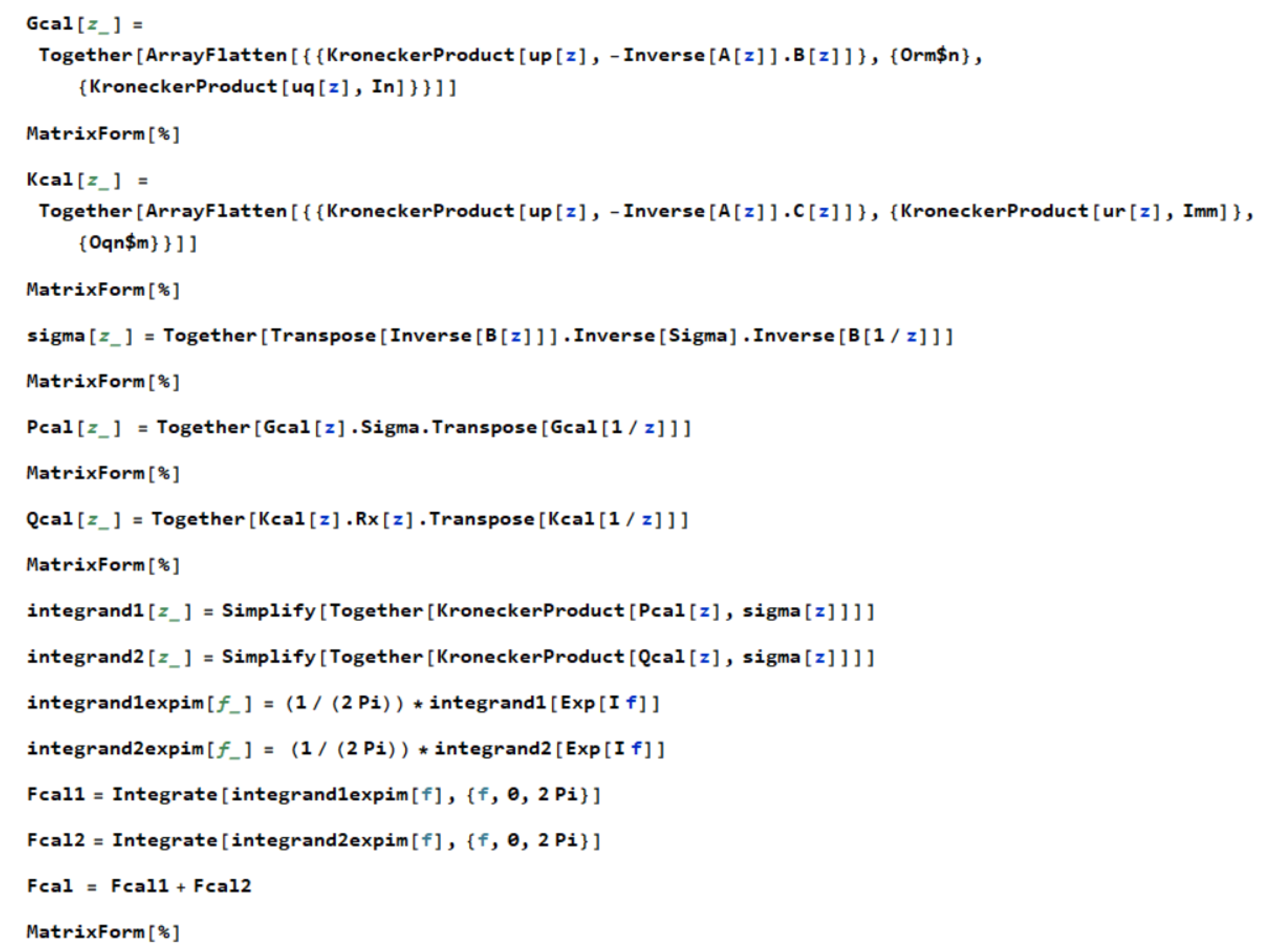
We propose an algorithm based on the method in the previous section and an implementation as a notebook for Mathematica. To make use of exact computations, the coefficients of the VARMAX model as well as $\mathsf{\Sigma }$ and $R_x$ are entered as fractions, if possible. The algorithm is provided in Figure 1 using some notations that are detailed here.

The arguments $\left(z\right)$ are written [z] for the polynomials. Given the polynomial matrices $A\left(z\right)$, $B\left(z\right)$, and $C\left(z\right)$ (hence denoted A[z], B[z], and C[z], respectively, in Figure 1), the vectors $u_p\left(z\right)$, $u_q\left(z\right)$, and $u_r\left(z\right)$ (denoted up[z], uq[z], and ur[z], respectively), the zero matrices $O_{rm\times n}$ and $O_{qn\times m}$ (denoted Orm$n and Oqn$m, respectively), the identity matrices $I_n$ and $I_m$ (denoted In and Imm, respectively, noting that Im is a locked symbol), plus $\mathsf{\Sigma }\left(z\right)$ (denoted Sigma[z]) and $R_x\left(z\right)$ (denoted Rx[z]). Then, the block matrices $\mathcal{G}\left(z\right)$ (Gcal[z]) and $\mathcal{K}\left(z\right)$ (Kcal[z]), are computed using the ArrayFlatten command of Mathematica, plus KroneckerProduct and Inverse, then $\sigma \left(z\right)$ (sigma[z]), $\mathcal{P}\left(z\right)$ (Pcal[z]), and $\mathcal{Q}\left(z\right)$ (Qcal[z]) using also the Transpose function. Since Mathematica does not treat well circular integrals, we transform them into line integrals between 0 and $2\pi$ by using the change of variable $z=e^{if}$, $0\le f\le 2\pi$, hence $dz/z=idf$. We compute the two transformed integrals of matrices using the command Integrate and sum them up. Contrary to the computations in (Appendix B, [7]), where individual formulas (taken from [18]) were used for each element and computed using the Cauchy rule, here the (two) integrals of the whole matrices are computed symbolically. To simplify the expressions as much as possible as rational functions of z, we use several times the commands Together and also Simplify. 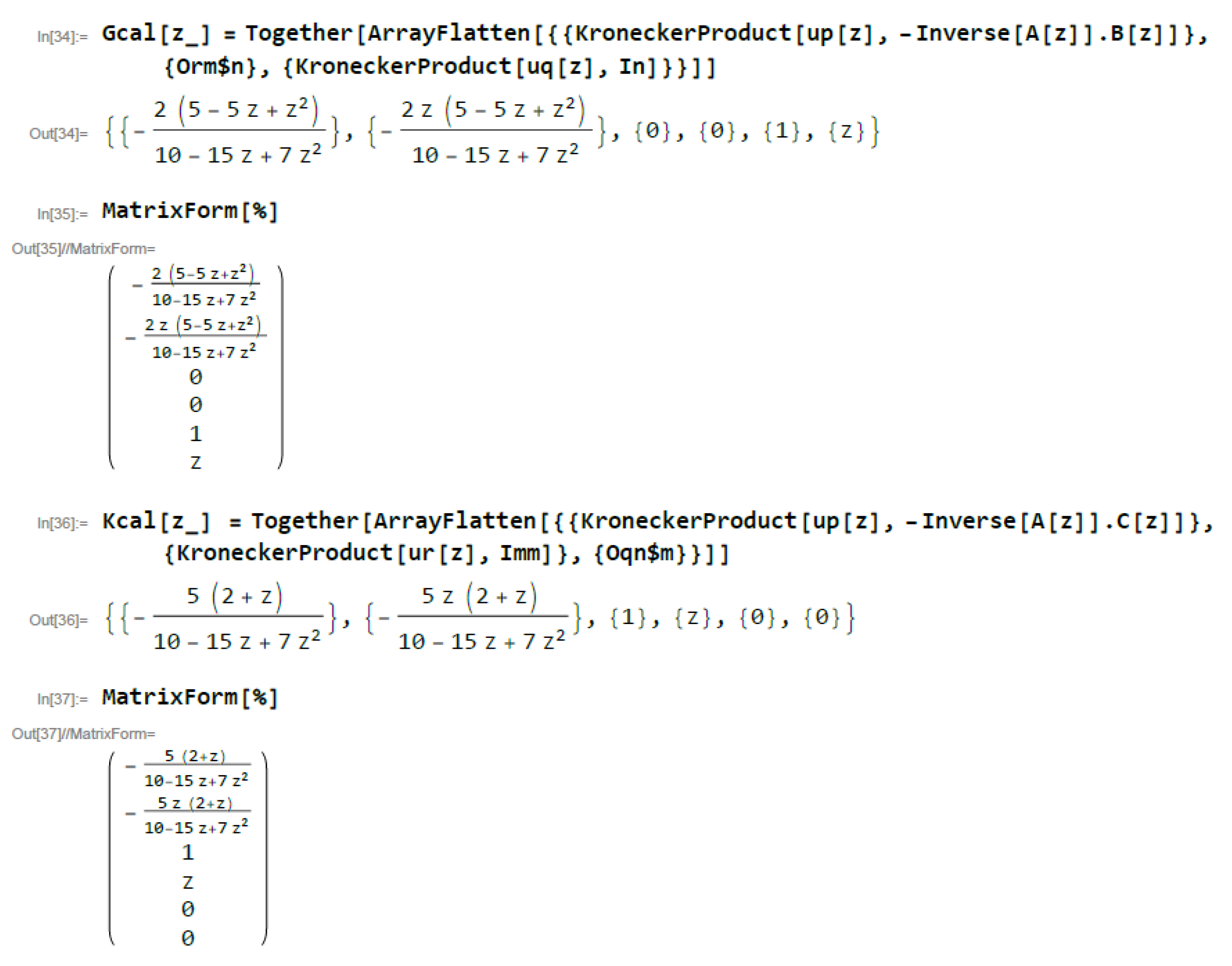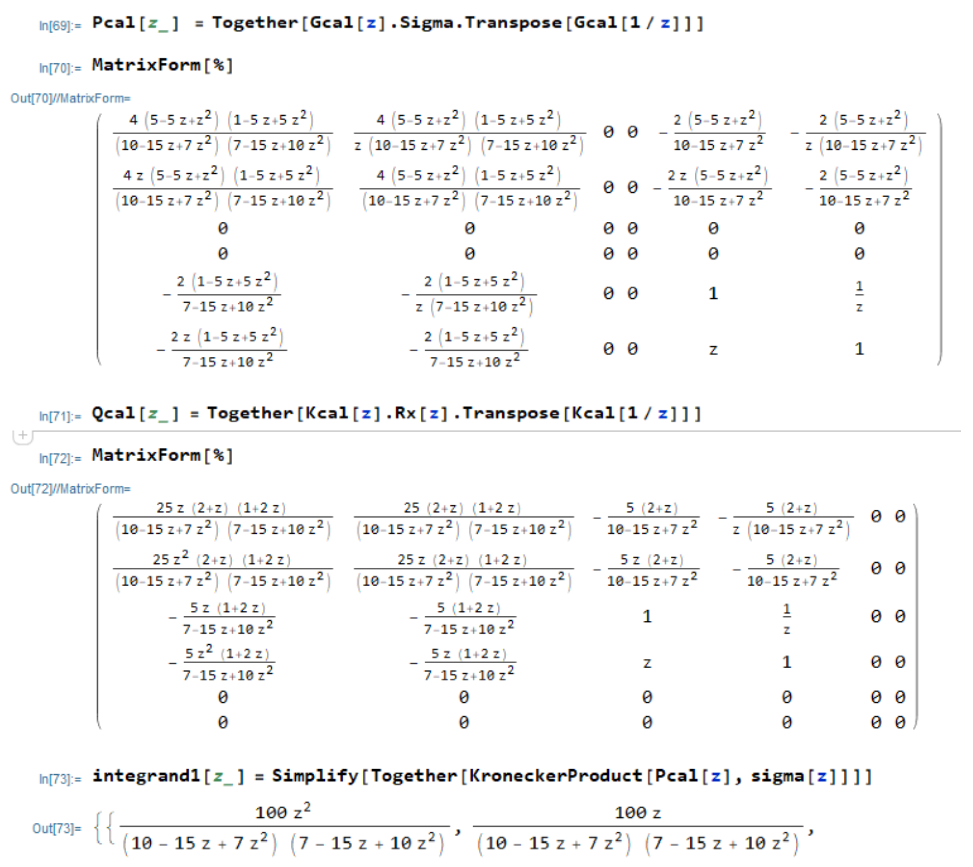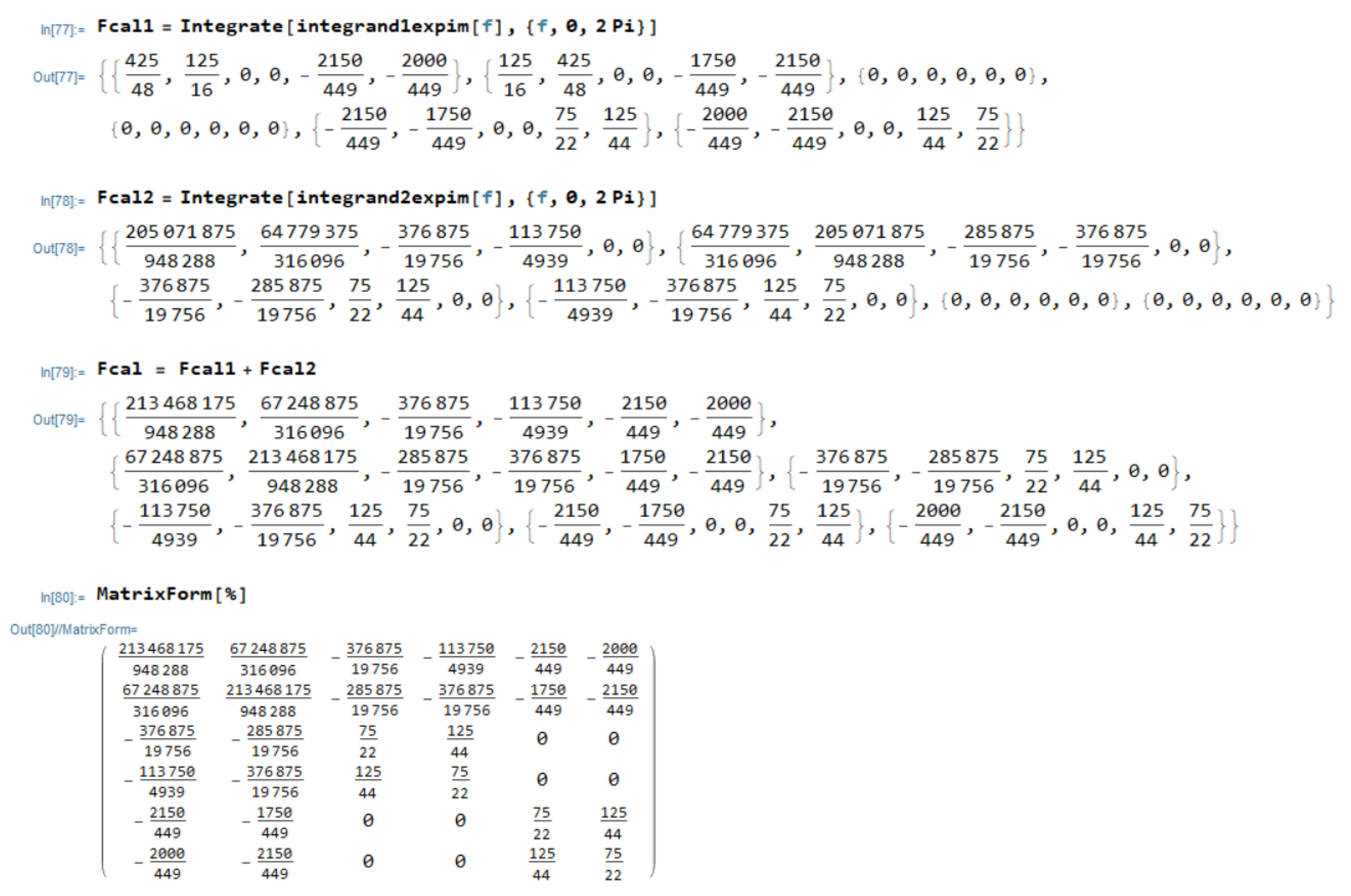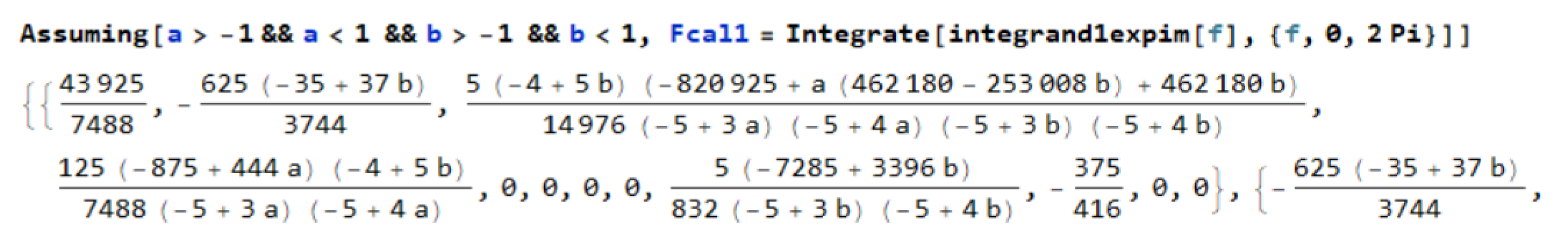The algorithm is shown in Figure 1 as a Mathematica notebook. The example is related to a VARMAX model used by [31] and also used by [32]. The model is defined by:

$$(1-1.5z+0.7z^2)y_t=(1+0.5z)x_t+(1-z+0.2z^2){\epsilon }_t.$$

(10)

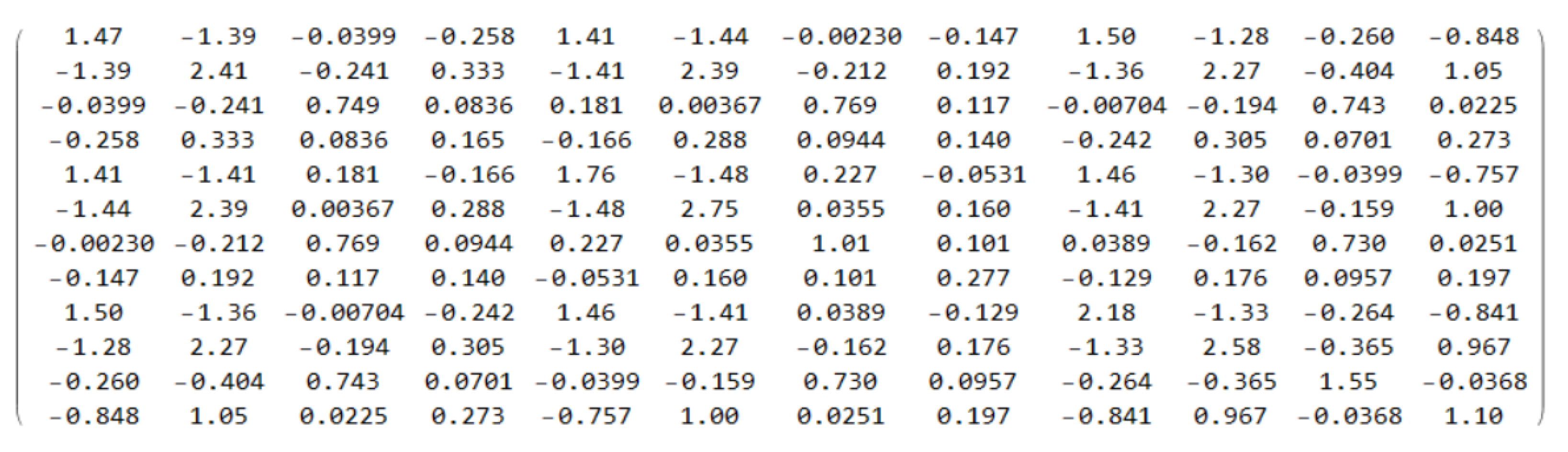
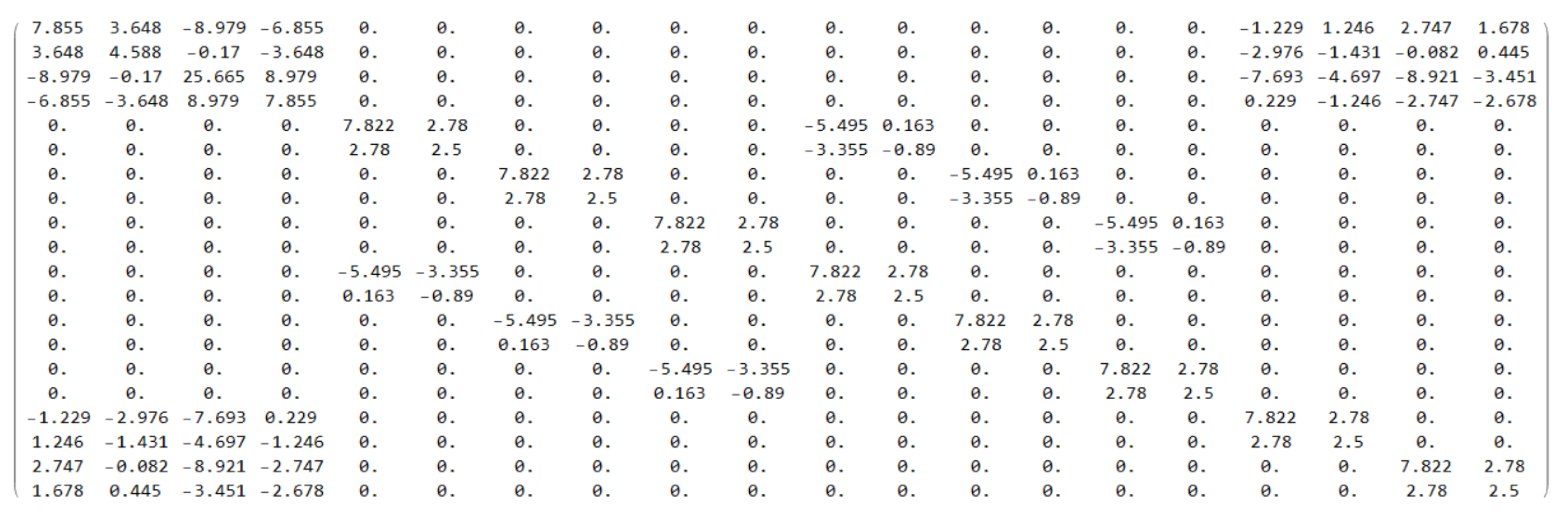
The coefficients are entered as fractions, hence $A_1=-3/2$, $A_2=7/10$, $C_0=1$, $C_1=1/2$, $B_1=-1$, and $B_2=1/5$. Part of the results are thus shown in Figure 2, Figure 3 and Figure 4. It took about 7.2 min to produce the output. Making the computation using the numerical program described in [32] on the same computer took 30 s but for one million evaluations.

Supplementary Materials Supplementary S1 contains the corresponding notebook (Figure1234.nb) that can be read using the free Wolfram’s CDF Player and its PDF copy (Figure1234.pdf). We will show and discuss other examples in the next Section. Note that we tried to implement the algorithm in two open-source packages for symbolic computation, Octave and Maxima. It is feasible because both programs allow us to integrate matrices but it appears that there is an error in the computation of the integrals being involved. We have informed the respective developers of the bug but the errors are not corrected yet.

Before showing other examples, let us look at other algorithms published in the literature. As said already, most of them are for the exact Fisher information, not the asymptotic Fisher information and we will not discuss them here, focusing instead on the asymptotic information matrix. Note that none of the existing algorithms is developed for VARMAX models, but only for VARMA or univariate models.

The first algorithm was due to Newton [16] for VARMA models. It is based on [22] who expressed the information matrix by a trigonometric integral involving the derivatives of the spectral density matrix of the process with respect to the parameters. The spectral density at frequency f, $f\in [-\pi ,\pi ]$, of a VARMAX process, e.g., (1) without the term ${\sum }_{j=0}^{r-1}{C}_j{x}_{t-j}$, is given by $(1/2\pi )A^{-1}\left(e^{if}\right)B\left(e^{if}\right)\mathsf{\Sigma }{B}^{\ast }\left(e^{if}\right)A^{\ast -1}\left(e^{if}\right)$. Newton [16] does not indicate how to evaluate these matrix integrals that he obtained. It can be seen that the integrand of each element of these matrix integrals is a rational function of $e^{if}$. Furthermore, the condition of stationarity implies that the denominator has a factor with zeroes in the unit circle and zeroes outside of it. Peterka and Vidinčev [33] have proposed an algorithm for evaluating circular integrals of a rational function around the unit circle and [34] has proposed an implementation that consists of a series of reduction in the degrees of the involved polynomials. That method was used by [12] for the evaluation of the Fisher information matrix of ARMA models.

A completely different early and effective method but restricted to ARMA models was proposed by Godolphin and Unwin [11]. It makes use of simple matrix operations with the inversion of two matrices, one of order p and one of order q.

Another approach was proposed by [35] which consists of replacing the computation of the integral by the evaluation of the cross-covariance of two ARMA processes based on the same white noise process, and this problem can be transformed in the computation of the autocovariance of a single AR process. There are excellent algorithms for that computation due to [36,37]. They require a number of operations which is quadratic in the AR order, much less than previous algorithms where a matrix of that order had to be inverted. The first algorithm was used by [13] for the evaluation of the Fisher information matrix of seasonal ARMA models. Ref. [38] have complained that several high-order AR models are sometimes involved and have proposed an alternative approach. Nevertheless, the algorithm making use of the autocovariances of an AR process using [37] could be developed for SISO models [15] and even for seasonal SISO models [32]. For ARMAX models, ref. [14] did not insist on algorithms but more on checking the invertibility of the Fisher information matrix, the subject of the next section. For ARMAX or SISO models, the Fisher information matrix is a sum of two integrals. The approach has however reached its limitations because the construction of the polynomials involved in the procedure becomes complex. For instance, the algorithm in [32] made use of a table with letters identifying the regular polynomials (a to f) and the seasonal polynomials (A to F) among others (the constant and the regression coefficient) involved as numerators or denominators in the different integrals. For a VARMAX model, there are 3 polynomials, hence the information matrix is a $3\times 3$ block matrix with, according to symmetry, 6 different blocks, including 1 corresponding to the parameters in the $A_j$ where a sum of two integrals appears. A simple inspection of the expressions for the different blocks in [18] reveals that obtaining the polynomials is a complex task.

4. A Sufficient Condition of Identifiability

The conditions for the identifiability of a VARMAX model have been studied by [25], among others. They are repeated later. A clear indication of identifiability is the invertibility of the Fisher information matrix. In this section, we derive a sufficient condition of invertibility for the case where $m=n$ and we enforce that the condition is not necessary, as could be deduced from the wrong arguments of [17]. For an ARMAX model, i.e., when $n=m=1$, [14] proved that a necessary and sufficient condition for invertibility of the Fisher information matrix is that the three polynomials have no common root. Indeed, as will be seen, the result of [14] cannot be extended to vector processes.

We have already been reminded of the concepts of reciprocal polynomials and eigenvalues of matrix polynomials. There remains to define what are a unimodular polynomial matrix and the common left divisor of matrix polynomials, see, e.g., [39].

A unimodular polynomial matrix $U\left(z\right)$ is a polynomial square matrix such that its determinant is a non-zero constant, instead of being a polynomial in z. Consequently, $U^{-1}\left(z\right)$ is also a polynomial matrix. In general, the inverse of a square polynomial matrix is a matrix with rational elements, not polynomial elements.

Three matrix polynomials $A\left(z\right)$, $B\left(z\right)$, and $C\left(z\right)$ with the same number of rows n have a common left divisor if there exist $n\times n$ polynomial matrices $F\left(z\right)$, $A^{\prime }\left(z\right)$, $B^{\prime }\left(z\right)$, and $C^{\prime }\left(z\right)$, such that $A\left(z\right)=F\left(z\right)A^{\prime }\left(z\right)$, $B\left(z\right)=F\left(z\right)B^{\prime }\left(z\right)$, and $C\left(z\right)=F\left(z\right)C^{\prime }\left(z\right)$. In matrix form, we can write $\left(A\left(z\right)B\left(z\right)C\left(z\right)\right)=F\left(z\right)\left(A^{\prime }\left(z\right)B^{\prime }\left(z\right)C^{\prime }\left(z\right)\right)$. Then $\left(A\right(z\left)B\right(z\left)C\right(z\left)\right)$ is called a right multiple of $F\left(z\right)$. A left divisor $F\left(z\right)$ is called the greatest common left divisor of $\left(A\right(z\left)B\right(z\left)C\right(z\left)\right)$ if it is a right multiple of all left divisors. Multiplying a greatest common left divisor to the right by any unimodular polynomial matrix yields another greatest common left divisor. As indicated by (Section 2.2, [25]), a greatest common left divisor can be constructed by elementary column operations: interchange any two columns, multiply any column by a real number different from 0, and add a polynomial multiple of any column to any column. Also, it corresponds to the right multiplication of $\left(A\right(z\left)B\right(z\left)C\right(z\left)\right)$ by an appropriate unimodular matrix. The concept can also be defined for rectangular matrices with the same number of rows although we will not consider that generalization.

Lemma 1. 

Assume that $A\left(z\right)$, $B\left(z\right)$, and $C\left(z\right)$ have the prescribed degrees, respectively, p, q, and $r-1$, with $\det \left(A\right(z\left)\right)\ne 0$ and $\det \left(B\right(z\left)\right)\ne 0$, for z in the unit circle of $\mathbb{C}$, and $\mathsf{\Sigma }$ is non-singular. Assume also that $x_t$ has an absolutely continuous spectrum with spectral-density non-zero on a set of positive measure on $(-\pi ,\pi ]$. Then a necessary and sufficient condition of identifiability of a stationary VARMAX process satisfying (1) is (i) $A\left(z\right)$, $B\left(z\right)$, and $C\left(z\right)$ have $I_n$ as greatest common left divisor, (ii) the matrix $\left(A_p{B}_q{C}_{r-1}\right)$ has rank n.

Proof. 

Since $\mathsf{\Sigma }$ is non-singular and given the assumptions on $A\left(z\right)$ and $B\left(z\right)$, the conditions (8a), (8b), and (8c) of [40] are satisfied for $A^{-1}\left(z\right)B\left(z\right)$, and the lemma is a special case of (Theorem 2, [40]) in the case (iii)${}_2$.  □

Since identifiability is equivalent to the inversibility of the Fisher information matrix, we are interested in finding a sufficient condition for identifiability. Equivalently, we are looking for a simple necessary condition for the lack of identifiability or the singularity of the Fisher information matrix, when $m=n$.

We can state the following theorem.

Theorem 1. 

Under the assumptions of Lemma 1 and if $m=n$, a sufficient condition of invertibility of the Fisher information matrix, $\mathcal{F}\left(\vartheta \right)$, associated with the VARMAX model with the matrix polynomials $A\left(z\right),C\left(z\right)$, and $B\left(z\right)$ of degree $p,r-1,q$, respectively, is that the reciprocal matrix polynomials $\tilde{A}\left(z\right)$, $\tilde{B}\left(z\right)$, and $\tilde{C}\left(z\right)$ have no common eigenvalue.

Proof. 

If the lack of identifiability occurs because (i) in Lemma 1 is not satisfied, that means that there exists a non-unimodular polynomial matrix $F\left(z\right)$, i.e., with $\det \left(F\right(z\left)\right)$ different from a constant and matrices $A^{\prime }\left(z\right)$, $B^{\prime }\left(z\right)$, and $C^{\prime }\left(z\right)$, such that $\left(A\left(z\right)B\left(z\right)C\left(z\right)\right)=F\left(z\right)\left(A^{\prime }\left(z\right)B^{\prime }\left(z\right)C^{\prime }\left(z\right)\right)$. Since the three polynomial matrices are square, we can consider their determinant stored in a row vector for which

$$\left(\det \left(A\left(z\right)\right)\det \left(B\left(z\right)\right)\det \left(C\left(z\right)\right)\right)=\det \left(F\left(z\right)\right)\left(\det \left(A^{\prime }\left(z\right)\right)\det \left(B^{\prime }\left(z\right)\right)\det \left(C^{\prime }\left(z\right)\right)\right),$$

where det$\left(F\right(z\left)\right)$ is a polynomial different from a constant. Hence, the equations det$\left(A\right(z\left)\right)=0$, det$\left(B\right(z\left)\right)=0$, and det$\left(C\right(z\left)\right)=0$ have at least one common root. Consequently, the matrix polynomials $A\left(z\right)$, $B\left(z\right)$, and $C\left(z\right)$ have at least one common eigenvalue. The same is also true for the reciprocal matrix polynomials $\tilde{A}\left(z\right)$, $\tilde{B}\left(z\right)$, and $\tilde{C}\left(z\right)$.

Now, if the lack of identifiability occurs because (ii) in Lemma 1 is not satisfied, that means that the matrix $\left(A_p{B}_q{C}_{r-1}\right)$ has a rank strictly smaller than n. Consequently, row n, say, of that matrix is a linear combination of the other $n-1$ rows and the matrices $A_p$, $B_q$, and $C_{r-1}$ do not have full rank. Hence the determinants det$\left(A\right(z\left)\right)$, det$\left(B\right(z\left)\right)$, and det$\left(C\right(z\left)\right)$ are polynomials of degree strictly smaller than, respectively, $np$, $nq$, and $n(r-1)$. Each of the reciprocal matrix polynomials $\tilde{A}\left(z\right)$, $\tilde{B}\left(z\right)$, and $\tilde{C}\left(z\right)$ have at least an eigenvalue equal to 0, hence at least one common eigenvalue.  □

Note that [17] has implicitly assumed that the determinants of $A\left(z\right)$ and $B\left(z\right)$ have their maximum degrees. For a discussion of identifiability without co-primeness, see [41]. For VARMA models, Ref. [24] has shown that it is not true to say, as [17] did, that the conditions in Theorem 1 are also necessary for invertibility of the Fisher information matrix. The approach of [17] used tensor Sylvester matrices which are a generalization of Sylvester matrices for the case of matrix polynomials instead of scalar polynomials. Consequently, the expectations of [19] mentioned in the second paragraph of Section 1 are not met for VARMAX models. Moreover, since there are three matrix polynomials and $C\left(z\right)$ does not need to be a square matrix, the tensor Sylvester matrices are not useful. It is also not useful to detail the alternative representations to (6) developed in (Sections 2.4 to 2.7, [19]) using the tensor Sylvester matrices. Let us just say that these representations seem to be correct in the sense that we have checked on all our examples for which $m=n$ that the Fisher information matrix obtained using them is identical to what is obtained using (7)–(9).

5. Numerical Experiments

The approach developed above can be used for any VARMAX model, for instance, the one produced by [42] obtained using a least-squares-based iterative estimation method.

To save space, we will use examples based on the simplest case, i.e., $n=m=2$, $C_0=I_2$, and $p=r=q=1$. We denote simply $A=A_1$, $B=B_1$, and $C=C_1$. For our first three examples, we will have:

$$R_x=\left(\begin{array}{cc}2.0& 0.0\\ 0.0& 3.0\end{array}\right),\mathsf{\Sigma }=I_2.$$

Example 1. 

Let A, B, and C be defined by

$$A=\left(\begin{array}{cc}-0.8& 0.0\\ -0.5& -a\end{array}\right),B=\left(\begin{array}{cc}-b& 0.0\\ -0.5& -0.6\end{array}\right),C=\left(\begin{array}{cc}-a& 0.0\\ -0.5& -0.7\end{array}\right),$$

where a and b are constants. The eigenvalues of $A\left(z\right)$, $B\left(z\right)$, and $C\left(z\right)$ are, respectively, the pairs $(0.8,a)$, $(0.6,b)$, and $(0.7,a)$ so that, whatever a and b, there is a common eigenvalue for $A\left(z\right)$ and $C\left(z\right)$. Clearly, the model is identifiable except if $a=b=0.8$ because then the factor $1-0.8z$ can be simplified on the first row of the system equation. In this case, because of the presence of the symbolic constants a and b, the algorithm needs to be changed by adding a command Assuming, as shown in Figure 5, with the mention that a and b are restricted to the interval $[-1,1]$. It is of course not possible to show here more of the matrix, see Supplementary Materials.

Take $b=0.8$ to simplify the discussion. Then, using Mathematica, it can be seen that the Fisher information matrix has a determinant proportional to $(4-5a)$ with a strictly positive factor, and indeed it is $0$ if, and only if, $a=0.8$. If $a=0.8$, the 2nd, 6th, and 10th rows of the Fisher information matrix contain the fractions

$$\mathit{Row}\mathit{2}=\left(\frac{1125}{416},\frac{75}{16},0,0,-\frac{375}{208},-\frac{25}{8},0,0,-\frac{375}{416},-\frac{25}{16},0,0\right),$$

$$\mathit{Row}\mathit{6}=\left(-\frac{375}{208},-\frac{25}{8},0,0,\frac{375}{208},\frac{25}{8},0,0,0,0,0,0\right),$$

$$\mathit{Row}\mathit{10}=\left(-\frac{375}{416},-\frac{25}{16},0,0,0,0,0,0,\frac{375}{416},\frac{25}{16},0,0\right),$$

and it is easy to check that −Row2 = −Row6 − Row10. Since the asymptotic information matrix is singular, there is no need to show it.

As we said, the computations described in Section 3 were implemented as matrix computations in Mathematica with coefficients given in the fractional form (e.g., 8/10 instead of 0.8) to have exact results. The complete Mathematica notebook (Example51.nb) is provided as Supplementary Materials, with its PDF output (Example51.pdf).

Example 2. 

Let A, B, and C be defined by:

$$A=\left(\begin{array}{cc}0.6& 0.2\\ 0.0& 0.0\end{array}\right),B=\left(\begin{array}{cc}0.5& 0.76\\ 0.0& 0.0\end{array}\right),C=\left(\begin{array}{cc}0.8& 0.0\\ 0.0& 0.0\end{array}\right).$$

This example is a generalization of a VARMA model considered by [24] based on an example in [43]. The determinants of $A\left(z\right)$, $B\left(z\right)$, and $C\left(z\right)$ have degree $1$, so we need to consider the reciprocal matrix polynomials $\tilde{A}\left(z\right)$, $\tilde{B}\left(z\right)$, and $\tilde{C}\left(z\right)$ which have respective roots $(-0.6,0)$, $(-0.5,0)$, and $(-0.8,0)$. Hence, we can consider the singularity of the Fisher information matrix. This is confirmed by computation with Mathematica which shows that the matrix has rank 10. Moreover, rows 3, 4, 7, 8, 11, and 12 of the Fisher information matrix contain the fractions

$$\mathit{Row}3=\left(\frac{4}{105},\frac{38}{2625},\frac{16}{3},\frac{152}{75},0,0,-4,-\frac{38}{25},0,0,-\frac{4}{3},-\frac{38}{75}\right)$$

$$\mathit{Row}4=\left(\frac{152}{2625},\frac{1444}{65625},\frac{152}{75},\frac{13276}{1875},0,0,-\frac{38}{25},-\frac{3319}{625},0,0,-\frac{38}{75},-\frac{3319}{1875}\right)$$

$$\mathit{Row}7=\left(-\frac{4}{7},-\frac{38}{175},-4,-\frac{38}{25},0,0,4,\frac{38}{25},0,0,0,0\right)$$

$$\mathit{Row}8=\left(-\frac{152}{175},-\frac{1444}{4375},-\frac{38}{25},-\frac{3319}{625},0,0,\frac{38}{25},\frac{3319}{625},0,0,0,0\right)$$

$$\mathit{Row}11=\left(\frac{8}{15},\frac{76}{375},-\frac{4}{3},-\frac{38}{75},0,0,0,0,0,0,\frac{4}{3},\frac{38}{75}\right)$$

$$\mathit{Row}12=\left(\frac{304}{375},\frac{2888}{9375},-\frac{38}{75},-\frac{3319}{1875},0,0,0,0,0,0,\frac{38}{75},\frac{3319}{1875}\right)$$

and it appears that Row3 = − Row11 − Row7 and Row4 = − Row8 − Row12.

Example 3. 

Let A, B, and C be defined by

$$A=\left(\begin{array}{cc}0.6& 0.2\\ 0.4& -0.6\end{array}\right),B=\left(\begin{array}{cc}0.5& 0.76\\ 0.25& -0.5\end{array}\right),C=\left(\begin{array}{cc}0.7& 0.1\\ -0.5& -0.7\end{array}\right).$$

(11)

This example is a generalization of the bivariate VARMA(1,1) model in (Example 1, [17]). There, the two matrix polynomials had the same two eigenvalues. In [17], it was concluded, wrongly, that the Fisher information matrix should be singular although the numerical computations in Matlab lead to the smallest eigenvalue equal to $0.0067$. This incoherency was explained by numerical inaccuracy. In [24], Mélard gave a second view to that example and discovered that the necessity and sufficiency of invertibility of the Fisher information matrix is only a necessary condition. For the VARMAX model related to (11), the three matrix polynomials have the same eigenvalues $\pm 5/\sqrt{11}$. Exact computations with Mathematica indicate, however, that the determinant of the $12\times 12$ Fisher information matrix is strictly positive and that the smallest eigenvalue is $0.0919$. The inverse of the asymptotic Fisher information matrix is shown in Figure 6. This example provides a counter-example that the sufficient condition in Theorem 1 is not necessary.

Example 4. 

This example is based on the example in (Section 4.1, [7]) so with $n=2$, $m=3$, $p=q=r=1$, $\mathsf{\Sigma }=I_2$, and $R_x\left(z\right)=I_3$. Let $A_1=O_{2\times 2}$, $C_0=C_1=O_{2\times 3}$, and $B_1$ be defined by:

$$B_1=\left(\begin{array}{cc}6/5& 1/2\\ -7/5& -1/5\end{array}\right).$$

(12)

The total number of parameters is $4+6+6+4=20$. In (Section 4.1, [7]), the exact Fisher information matrix was computed and compared to those obtained using the E4 Toolbox for Matlab, see [5,44], but (Appendix B, [7]) contains the results for the asymptotic Fisher information matrix obtained using individual formulas in [18] for each of the 10 different blocks, the computation of the integrals being performed using the algorithm in [33]. Here, we do not bother with complex individual expressions and the computation of integrals. We simply use the notebook described in Figure 1 and adapt the model specifications. See the resulting information matrix in Figure 7.

6. Conclusions

In this paper, we have proposed for the first time an exact method to compute the asymptotic Fisher information matrix of VARMAX processes, an algorithm for symbolic computation software, and an implementation for Mathematica. It is based on an extension of the method proposed in [19].

Therefore, we could not compare it with other algorithms in the general case. Nevertheless, we could compare it to the special case of an ARMAX process where there exists alternative algorithms.

The open-source packages Octave and Maxima should be able to do the job since their symbolic integration procedure can work on matrices of functions, but they do not work presently. More developments would be needed to circumvent their failing integration.

We also provide a simple sufficient condition of invertibility of the asymptotic Fisher information matrix and Example 3 shows that the condition is not necessary.

We did not examine the complexity of our algorithm because the concept is not well-established for symbolic computation. Let us just say that, at this stage, it will take much more running time, as seen in the special case discussed in Section 3. For instance, the timings given for the ARMAX model of Section 3 show that the numerical method is considerably faster. Also, the program implementing the algorithm relies on the capabilities of the symbolic computation package and possible hardware and software limitations. This is the price to pay for the ability to provide exact results, at least when the matrix entries are given as fractions, not as decimal numbers. We believe, however, that the fact that, when it works at least, the notebook that we have produced the result for an arbitrary VARMAX model.

We should conclude with possible extensions of our results. There have been papers on the asymptotic information matrix for extended models like ARMA models with periodic coefficients [45,46], state-space models [46], Markov switching VARMA models [47], or VARFIMA models [48]. It is possible that the approach described in this paper can be extended to these extended models.

References

1. Lütkepohl, H. Introduction to Multiple Time Series Analysis; Springer: New York, NY, USA, 1991. [Google Scholar]
2. Porat, B.; Friedlander, B. Computation of the exact information matrix of Gaussian time series with stationary random components. IEEE Trans. Acoust. Speech Signal Process. 1986, 14, 118–130. [Google Scholar] [CrossRef]
3. Zadrozny, P.A. Analytical derivatives for estimation of linear dynamic models. Comput. Math. Appl. 1989, 18, 539–553. [Google Scholar]
4. Terceiro Lomba, J. Estimation of Dynamic Econometric Models with Errors in Variables; Springer: Berlin/Heidelberg, Germany, 1990. [Google Scholar]
5. Casals, J.; Sotoca, S. Exact initial conditions for maximum likelihood estimation of state space models with stochastic inputs. Econ. Lett. 1997, 57, 261–267. [Google Scholar] [CrossRef]
6. Jerez, M.; Casals, J.; Sotoca, S. Signal Extraction for Linear State-Space Models; Lambert Academic Publishing: Saarbrücken, Germany, 2011. [Google Scholar]
7. Klein, A.; Mélard, G. An algorithm for the exact Fisher information matrix of vector ARMAX time series. Linear Algebra Appl. 2014, 446, 1–24. [Google Scholar] [CrossRef]
8. Bao, Y.; Hua, Y. On the Fisher information matrix of a vector ARMA process. Econ. Lett. 2014, 123, 14–16. [Google Scholar] [CrossRef]
9. Dharan, B.G. A priori sample size evaluation and information matrix computation for time series models. J. Stat. Comput. Simul. 1985, 21, 171–177. [Google Scholar] [CrossRef]
10. Box, G.E.P.; Jenkins, G.M.; Reinsel, G.C.; Ljung, G.M. Time Series Analysis Forecasting and Control, 5th ed.; Wiley: Hoboken, NJ, USA, 2015. [Google Scholar]
11. Godolphin, E.J.; Unwin, J.M. Evaluation of the covariance matrix for the maximum likelihood estimator of a Gaussian autoregressive-moving average process. Biometrika 1983, 70, 279–284. [Google Scholar] [CrossRef]
12. Klein, A.; Mélard, G. On algorithms for computing the covariance matrix of estimates in autoregressive-moving average models. Comput. Stat. Q. 1989, 5, 1–9. [Google Scholar]
13. Klein, A.; Mélard, G. Fisher’s information matrix for seasonal autoregressive-moving average models. J. Time Ser. Anal. 1990, 11, 231–237. [Google Scholar] [CrossRef]
14. Klein, A.; Spreij, P. On Fisher’s information matrix of an ARMAX process and Sylvester’s resultant matrices. Linear Algebra Appl. 1996, 237–238, 579–590. [Google Scholar] [CrossRef]
15. Klein, A.; Mélard, G. Computation of the Fisher information matrix for SISO models. IEEE Trans. Signal Process. 1994, 42, 684–688. [Google Scholar] [CrossRef]
16. Newton, H.J. The information matrices of the parameters of multiple mixed time series. J. Multivar. Anal. 1978, 8, 317–323. [Google Scholar] [CrossRef] [Green Version]
17. Klein, A.; Mélard, G.; Spreij, P. On the resultant property of the Fisher information matrix of a vector ARMA process. Linear Algebra Appl. 2005, 403, 291–313. [Google Scholar] [CrossRef] [Green Version]
18. Klein, A.; Spreij, P. Matrix differential calculus applied to multiple stationary time series and an extended Whittle formula for information matrices. Linear Algebra Appl. 2009, 430, 674–691. [Google Scholar] [CrossRef]
19. Klein, A.; Spreij, P. Tensor Sylvester matrices and the Fisher information matrix of VARMAX processes. Linear Algebra Appl. 2010, 432, 1975–1989. [Google Scholar] [CrossRef]
20. Zadrozny, P.A. Errata to ‘Analytical derivatives for estimation of linear dynamic models’. Comput. Math. Appl. 1992, 24, 289–290. [Google Scholar]
21. Mittnik, S.; Zadrozny, P.A. Asymptotic distributions of impulse responses, step responses, and variance decompositions of estimated linear dynamic model. Econometrica 1993, 61, 857–870. [Google Scholar] [CrossRef]
22. Whittle, P. Estimation and information in time series. Ark. Mat. 1953, 2, 423–434. [Google Scholar] [CrossRef]
23. Gohberg, I.; Lerer, L. Resultants of matrix polynomials. Bull. Am. Math. Soc. 1976, 82, 565–567. [Google Scholar] [CrossRef] [Green Version]
24. Mélard, G. An indirect proof for the asymptotic properties of VARMA model estimators. Econom. Stat. 2022, 21, 96–111. [Google Scholar] [CrossRef]
25. Hannan, E.J.; Deistler, M. The Statistical Theory of Linear Systems; Wiley: New York, NY, USA, 1988. [Google Scholar]
26. Caines, P. Linear Stochastic Systems; Wiley: New York, NY, USA, 1988. [Google Scholar]
27. Brockwell, P.J.; Davis, R.A. Time Series: Theory and Methods, 2nd ed.; Springer: Berlin/Heidelberg, Germany, 1991. [Google Scholar]
28. Gohberg, I.; Lancaster, P.; Rodman, L. Matrix Polynomials; Academic Press: New York, NY, USA, 1982. [Google Scholar]
29. Brockwell, P.J.; Lindner, A.; Vollenbröker, B. Strictly stationary solutions of multivariate ARMA equations with i.i.d. noise. Ann. Inst. Stat. Math. 2012, 64, 1089–1119. [Google Scholar] [CrossRef] [Green Version]
30. Magnus, J.R.; Neudecker, H. Matrix Differential Calculus with Applications in Statistics and Econometrics; Wiley: New York, NY, USA, 1988. [Google Scholar]
31. Gevers, M.; Ljung, L. Optimal experiment designs with respect to the intended model application. Automatica 1986, 22, 543–544. [Google Scholar] [CrossRef]
32. Klein, A.; Mélard, G. An algorithm for computing the asymptotic Fisher information matrix for seasonal SISO models. J. Time Ser. Anal. 2004, 25, 627–648. [Google Scholar] [CrossRef]
33. Peterka, V.; Vidinčev, P. Rational-fraction approximation of transfer functions. In Proceedings of the IFAC Symposium on Identification in Automatic Control Systems, Prague, Czech Republic, 12–17 June 1967. [Google Scholar]
34. Söderström, T. Description of a Program for Integrating Rational Functions Around the Unit Circle; Technical Report 8467R; Department of Technology, Uppsala University: Uppsala, Sweden, 1984. [Google Scholar]
35. Pham, D.T. Cramér-Rao bounds for AR parameter and reflection coefficient estimators. IEEE Trans. Acoust. Speech Signal Process. 1989, 37, 769–772. [Google Scholar]
36. Tunnicliffe Wilson, G.T. Some efficient computational procedures for high order ARMA models. J. Stat. Comput. Simul. 1979, 8, 303–309. [Google Scholar] [CrossRef]
37. Demeure, C.J.; Mullis, C.T. The Euclid algorithm and the fast computation of cross-covariance and autocovariance sequences. IEEE Trans. Acoust. Speech Signal Process. 1989, 37, 545–552. [Google Scholar] [CrossRef]
38. Godolphin, E.J.; Bane, S.R. On the evaluation of the information matrix for multiplicative seasonal time series models. J. Time Ser. Anal. 2005, 27, 167–190. [Google Scholar] [CrossRef]
39. Hannan, E.J. The identification of vector mixed autoregressive-moving average systems. Biometrika 1969, 56, 223–225. [Google Scholar]
40. Hannan, E.J. The identification problem for multiple equation systems with moving average errors. Econometrica 1971, 39, 223–225. [Google Scholar] [CrossRef]
41. Wegge, L.L. Armax(p,r,q) Parameter Identifiablity without Coprimeness; Department of Economics Working Paper 12-17; University of California: Davis, CA, USA, 2012; Available online: https://www.researchgate.net/publication/254396797_ARMAXprq_Parameter_Identifiability_Without_Coprimeness (accessed on 19 May 2023).
42. Bao, B.; Xu, Y.; Sheng, J.; Ding, R. Least squares based iterative parameter estimation algorithm for multivariable controlled ARMA system modelling with finite measurement data. Math. Comput. Model. 2011, 53, 1664–1669. [Google Scholar] [CrossRef]
43. Athanasopoulos, G.; Vahid, F. VARMA versus VAR for macroeconomic forecasting. J. Bus. Econ. Stat. 2008, 26, 237–252. [Google Scholar] [CrossRef] [Green Version]
44. Terceiro, J.; Casals, J.M.; Jerez, M.; Serano, G.R.; Sotoca, S. Time Series Analysis Using MATLAB, Including a Complete MATLAB Toolbox. 2000. Available online: http://www.ucm.es/info/icae/e4 (accessed on 19 May 2023).
45. Bentarzi, M.; Aknouche, A. Calculation of the Fisher information matrix for periodic ARMA models. Commun. Stat. Theory Methods 2005, 34, 891–903. [Google Scholar] [CrossRef]
46. Hamdi, F. Computing the exact Fisher information matrix of periodic state-space models. Commun. Stat. Theory Methods 2012, 41, 4182–4199. [Google Scholar] [CrossRef]
47. Cavicchioli, M. Asymptotic Fisher information matrix of Markov switching VARMA models. J. Multivar. Anal. 2017, 157, 124–135. [Google Scholar] [CrossRef]
48. Contreras-Reyes, J.E. Rényi entropy and divergence for VARFIMA processes based on characteristic and impulse response functions. Chaos Solitons Fractals 2022, 160, 112268. [Google Scholar] [CrossRef]
Figure 1. Snapshot of the Mathematica notebook to treat a VARMAX model, given A[z], B[z], and C[z]. The result Fcal is F ( ϑ ) as defined in (9). See the text for the other notations.
Algorithms 16 00364 g001
Figure 2. Partial snapshot of the Mathematica notebook to treat the example in (10). Gcal[z] is G ( z ) and Kcal[z] is G ( z ) , both defined in (7).
Algorithms 16 00364 g002
Figure 3. Partial snapshot of the Mathematica notebook to treat the example in (10). Pcal[z] is P ( z ) and Qcal[z] is Q ( z ) , both defined in (8). To save space, only the first two elements of the first integrand in (9) are shown.
Algorithms 16 00364 g003
Figure 4. Partial snapshot of the Mathematica notebook to treat the example in (10). Fcal1 and Fcal2 are, respectively, the first and second terms in the right-hand side of (9) and Fcal is their sum, so equal to F ( ϑ ) .
Algorithms 16 00364 g004
Figure 5. Partial snapshot of the Mathematica notebook to treat Example 5.1. Note that the integration command is prefixed by a constraining assumption.
Algorithms 16 00364 g005
Figure 6. Output of the inverse of the Fisher information matrix for Example 3.
Algorithms 16 00364 g006
Figure 7. Output of the Fisher information matrix for Example 4.
Algorithms 16 00364 g007
Disclaimer/Publisher’s Note: The statements, opinions and data contained in all publications are solely those of the individual author(s) and contributor(s) and not of MDPI and/or the editor(s). MDPI and/or the editor(s) disclaim responsibility for any injury to people or property resulting from any ideas, methods, instructions or products referred to in the content.