Testing a New “Decrypted” Algorithm for Plantower Sensors Measuring PM_2.5: Comparison with an Alternative Algorithm

Abstract

Recently, a hypothesis providing a detailed equation for the Plantower CF_1 algorithm for PM_2.5 has been published. The hypothesis was originally validated using eight independent Plantower sensors in four PurpleAir PA-II monitors providing PM_2.5 estimates from a single site in 2020. If true, the hypothesis makes important predictions regarding PM_2.5 measurements using CF_1. Therefore, we test the hypothesis using 18 Plantower sensors from four datasets from two sites in later years (2021–2023). The four general models from these datasets agreed to within 10% with the original model. A competing algorithm known as “pm2.5 alt” has been published and is freely available on the PurpleAir API site. The accuracy, precision, and limit of detection for the two algorithms are compared. The CF_1 algorithm overestimates PM_2.5 by about 60–70% compared to two calibrated PurpleAir monitors using the pm2.5 alt algorithm. A requirement that the two sensors in a single monitor agree to within 20% was met by 85–99% of the data using the pm2.5 alt algorithm, but by only 22–74% of the data using the CF_1 algorithm. The limit of detection (LOD) of the CF_1 algorithm was about 10 times the LOD of the pm2.5 alt algorithm, resulting in 71% of the CF_1 data falling below the LOD, compared to 1 % for the pm2.5 alt algorithm.

1. Introduction

1.1. Low-Cost Optical Sensors

In recent years, there has been an explosion of interest in low-cost particle monitors. The fundamental question is accuracy. Accuracy can be determined under field conditions by comparison to nearby regulatory monitors employing the gravimetric-based Federal Reference Methods (FRM), which require collection of particles over 24 h followed by weighing filters under strict regulation of temperature and humidity. Since typically only one day out of every three can be monitored in this way, monitors were developed to estimate continuous variation of PM mass. The best of these monitors have passed stringent tests to determine their agreement with the FRM monitors. These monitors are called Federal Equivalence Monitors (FEM) and are in use at several hundred regulatory monitor sites in the United States. The accuracy of low-cost monitors can therefore be determined by comparing to either FRM or FEM monitors at regulatory sites. (For further information on the development of health standards such as PM_2.5 and PM₁₀, and the development of optical monitors, see Sections S1.0 and S1.1 of Supplementary Materials).

Accuracy can also be determined by laboratory or chamber investigations. In this approach, several monitors (usually in triplicate) to be tested are placed side by side with one or more reference monitors in a chamber with controlled temperature and humidity. A particle source (often organic PSL spheres, inorganic sodium chloride, or Arizona road dust) is activated and either maintained at a steady concentration or allowed to rise to a peak and then decay so that a wide variety of concentrations can be created.

A major source of both field and laboratory investigations of low-cost monitors is the program known as AQ-SPEC, operated by the South Coast Air Quality Management District (SCAQMD) in California. (This management district includes about 17 million people, 44% of the California population.) Monitors must pass a field test before being administered a chamber test. In the field, sensors are tested alongside one or more of South Coast AQMD’s existing air monitoring stations using traditional federal reference/equivalent method instruments over a 30- to 60-day period to gauge overall performance. Sensors demonstrating acceptable performance in the field are then brought to the AQ-SPEC laboratory for more detailed testing in an environmental chamber under controlled conditions alongside traditional federal reference/equivalent method and/or best available technology instruments [1].

About 100 field evaluation reports and 49 laboratory evaluation reports are presently available [2].

Both field and laboratory investigations of low-cost monitors have been carried out by multiple investigators [3,4,5,6,7,8,9,10,11,12,13,14,15,16,17,18,19,20,21,22,23,24,25]. Many of these involve Plantower sensors.

Plantower Sensors

This paper focuses on Plantower sensors. This focus is supported by the fact that 14 of 47 manufacturers of low-cost particle monitors tested in the AQ-SPEC program use Plantower sensors (

Table 1. Low-cost particle instruments using Plantower sensors tested in chamber studies by AQ-SPEC.

Instrument Tested by AQ-SPEC in Laboratory Report	Plantower Model
Airbeam 2	7003
Airbeam 3	7003
Air Quality Egg	5003
APT Minima	A003
AS-Lung	3003
Davis Instruments	A003
PurpleAir PM-I	1003
PurpleAir PM-II	5003
PurpleAir Flex	6003
Redspira	5003
Sain Smart	5003
Smart Citizen Kit	5003
Magna SCI SRL uRAD SMOGGIE	A003

). In addition, the largest national network of low-cost monitors (PurpleAir with perhaps 25,000 monitors) uses Plantower sensors exclusively.

1.2. Algorithms for Optical Particle Sensors

1.2.1. Standard Algorithm for Optical Particle Sensors

The standard algorithm employed by many manufacturers of optical particle counters since the 1970s is a completely open and transparent approach. It typically uses three bins (0.3–0.5 µm, 0.5–1 µm, and 1–2.5 µm) to calculate PM_2.5. For each bin, the assumption is made that all particles are spherical and have identical diameters D_p equal to some midpoint (either arithmetic or geometric mean) between the bin boundaries. The volume of the single particle is then πD_p³/6. All particles are assumed to have the same density ρ. The mass of the particle is then equal to the density multiplied by the volume: ρπD_p³/6. The total mass of particles in the bin is equal to the single-particle mass multiplied by the number N_i of particles in the bin. Finally, PM_2.5 is equal to the sum of the masses of all particles in the three bins:

PM_2.5 = aN1 + bN2 + cN3

(1)

where a, b, and c are simply the masses of the single (representative) particle in each bin and N1, N2, and N3 are the number of particles in each bin. Numerically, assuming the choice of geometric mean for the particle diameter and a density of 1 g cm⁻³, the values of a, b, and c are as follows (

Table 2. Calculation of the coefficients a, b, and c.

Bin	Dp (Geom. Mean) (µm)	Volume (µm3/100)	Mass (Density = 1) (µg/m3/100)
0.3–0.5 µm	0.387298335	0.000304183	a = 0.000304183
0.5–1 µm	0.707106781	0.001851201	b = 0.001851201
1–2.5 µm	1.58113883	0.020697059	c = 0.020697059

):

In this table, the volumes and masses have been divided by 100 since the number N_i of particles is in units of number per deciliter. This allows one to use the numbers reported by Plantower for N1, N2, and N3 without change.

Therefore, the alt PM_2.5 algorithm for a density of 1 g cm⁻³ is given by Equation (1) using the values of a, b, and c shown in the above table.

As with all uses of PM_2.5 estimates, however, it is always recommended that investigators compare the PM_2.5 predictions to research-grade instruments measuring the aerosol mixture of interest. In the field, this is usually done by comparing nearby regulatory monitors using gravimetric Federal Reference Method or continuous Federal Equivalence Method (FEM/FRM) to the aerosol mixture being measured. The result of the comparison is a calibration factor (CF) to adjust the PM_2.5 estimates. For the choice of geometric mean and density of 1 as mentioned above, the final equation for PM_2.5 becomes

PM_2.5 = CF(aN1 + bN2 +cN3)

(2)

1.2.2. Application of Standard Algorithm to Plantower Sensors

The standard algorithm in Equation (2) was first applied to Plantower PMS 5003 sensors used in PurpleAir PA-II monitors [4,19]. These studies tested 33 PurpleAir monitors within 500 m of 27 regulatory FEM/FRM monitors in California, finding the CF to be 3.0. The algorithm was therefore named ALT-CF3, where the “ALT” suggests an alternative algorithm to those supplied by Plantower and the “CF3” is the calibration factor found in these two studies. Therefore, the algorithm as applied to the PurpleAir monitors using Plantower PMS 5003 sensors is equal to

ALT-CF3 = 3(aN1 + bN2 + cN3)

(3)

where the a, b, and c coefficients are those in the above table.

This algorithm is freely available on the PurpleAir API site, where it has been renamed “pm2.5 alt”. A major study of 3000 indoor air monitors selected pm2.5 alt as the only algorithm to be used. The study is expected appear soon in Proceedings of the National Academy of Sciences (PNAS).

A more recent study showed that both the PMS 1003 and PMS 5003 sensors have an identical (within 2%) CF of 3.4 [20], leading to the revised Equation (3)

ALT-CF3.4 = 3.4(aN1 + bN2 + cN3)

(4)

where a, b, and c are still unchanged from the values in Table 2 above, but the CF is changed from 3 to 3.4.

This CF of 3.4 has been used in several studies and is used in this study as well. For persons wanting to use this most recent value, it is sufficient to multiply the value given in the API site by 3.4/3, or about a 12% increase in PM_2.5 values.

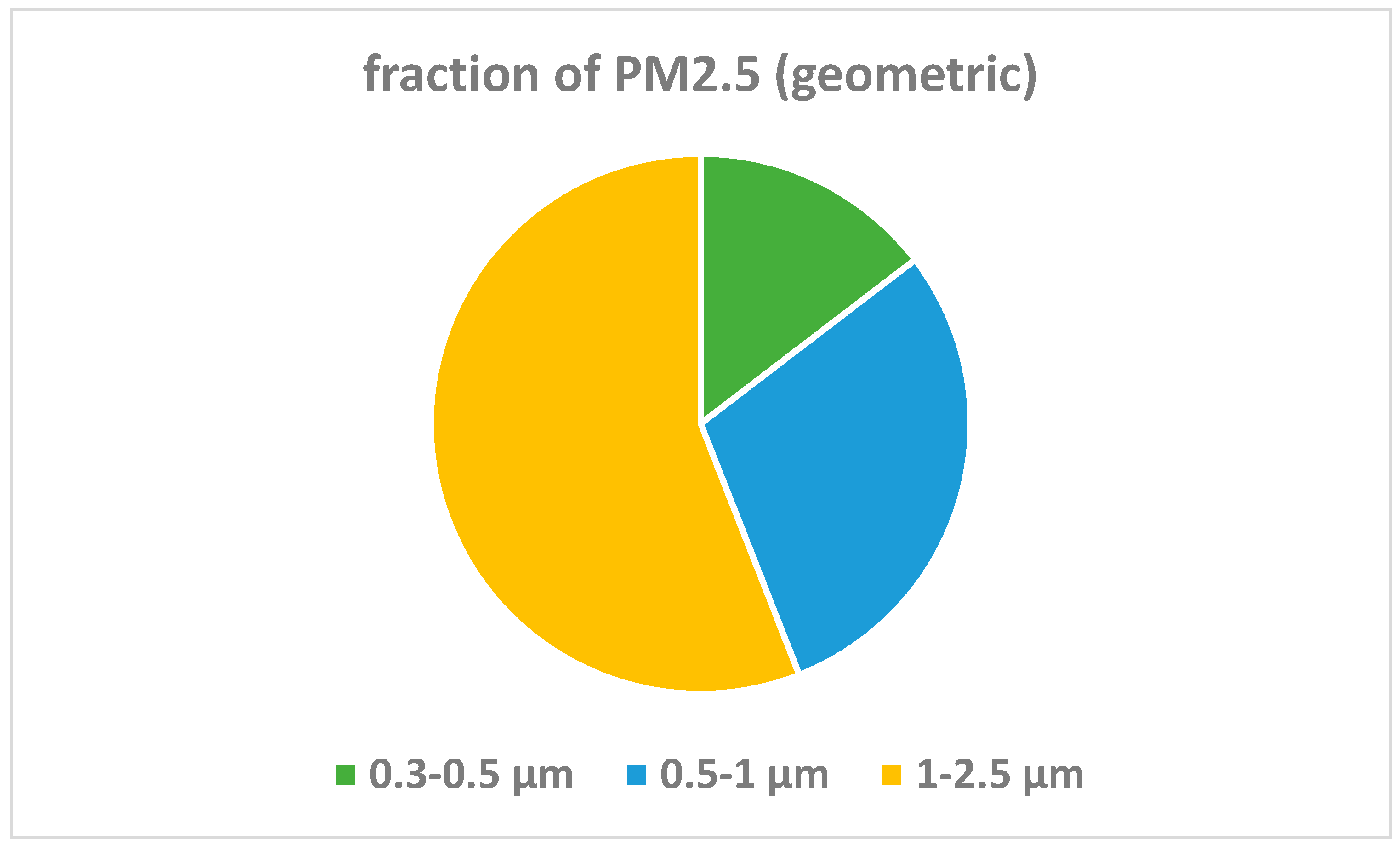
An advantage in using equations of the general form of Equation (2) above is that it allows an estimate of the contribution made by each size category to the total mass (PM_2.5). For example, typical values of N1, N2, and N3 occurring in a Santa Rosa home were determined from a full-year dataset from 1 January 2021 to 31 December 2021. These are entered into Equation (4) to determine the fractional contribution of each bin to total PM_2.5 during this period (

Table 3. Contribution of each bin to PM_2.5 over 1 year monitoring indoor particles.

Bin (µm)	Mass per Particle (µg/m3/100)	# Particles (Ni) per Deciliter	Mass per Bin (µg/m3)	Fraction of PM2.5
0.3–0.5	0.000304183	445	0.135	0.146
0.5–1	0.001851201	147	0.272	0.294
1–2.5	0.020697059	25	0.518	0.560

and Figure 1).

1.2.3. Algorithms Offered by Plantower

The Plantower manual v2.5 for the PMS 1003 sensor describes two algorithms for determining PM₁, PM_2.5, and PM₁₀. One algorithm is labeled as “CF = 1, standard particle”, the other as “under atmospheric environment”.

The Plantower manual v2.3 for the PMS 5003 sensor has the same labels for the two algorithms, but there is an added note for the CF1 algorithm: “CF = 1 should be used in the factory environment.”

Some have interpreted these cryptic descriptions as indicating that the CF = 1 algorithm should be used indoors and the “under atmospheric environment” algorithm should be used for outdoor measurements. However, Plantower presented no data to support their characterization of the two algorithms.

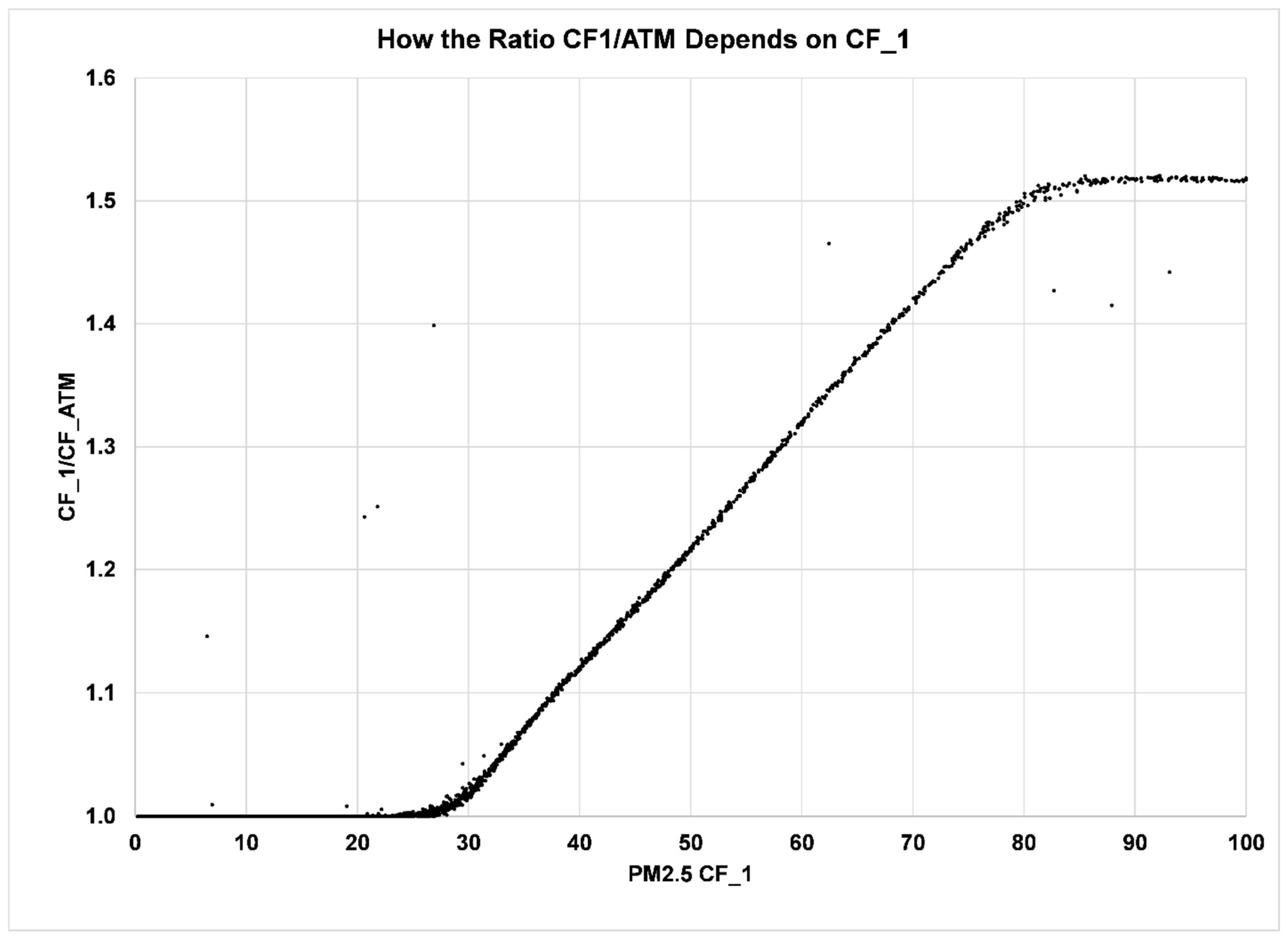
It is easy to determine the relation of the two algorithms. A 10-day run of data in a Santa Rosa home from 24 April 2019 to 3 May 2019 using a PurpleAir PA-II monitor gave these results for the relationship (Figure 2). It should be immediately evident that one of these two algorithms can have no physical reality; the relationship is simply a mathematical model. The two algorithms give identical results for all particle concentrations below about 28 µg/m³; a linear relation above that concentration, in which the CF_ATM/CF_1 ratio increases by about 0.01 unit for the next 50 steps of 1 µg/m³ for the CF_1 algorithm; and then, beginning at about 78 µg/m³, it curls over to become ultimately fixed at a constant ratio on the order of 1.5. No possible actual physical process could behave in this way. This observation by itself does not allow the problematic algorithm to be identified. However, based on correlations with measurements by other methods, the physically unrealizable algorithm is CF_ATM, which should, therefore, not be used (See Supplementary Materials Section S1.2 and Figures S1–S4). It is uncertain why this algorithm was developed, but the fact that the CF_1 algorithm is found by almost all investigators to overpredict PM mass may have caused the Plantower engineers to search for a new algorithm that would give better estimates. In fact, the CF_ATM algorithm does give lower estimates that may be closer to the truth, but for wrong reasons. Unfortunately, the PurpleAir corporation has chosen to adopt the CF_ATM algorithm for their outdoor map because it would partially correct the overestimate of the CF_1 algorithm. While this is true, at least for the small number of outdoor concentrations >28 µg/m³, it means that a meaningless algorithm is being used widely by >25,000 consumers with no indication of its lack of scientific basis. Several studies have concluded that the CF_1 algorithm should be used in place of the CF_ATM algorithm [9,18].

Danger of “Proprietary” Algorithms

Plantower presents no information regarding the composition, density, or index of refraction of the test aerosol used to calibrate its sensors. In fact, it does not even mention whether a test aerosol was used, or whether its instruments are calibrated. Its two algorithms are said to be “proprietary”, which seems contrary to the practice of earlier manufacturers, whose algorithms were openly described.

A problem with “proprietary” algorithms is the ever-present possibility that the manufacturer could change the algorithm at will. If the manufacturer does not announce that the algorithm has changed, consumers would not know a change had occurred, unless a careful examination of their historical data might reveal a change in some parameter (e.g., the relation of particle numbers in adjacent size categories). This is not only a theoretical possibility but actually occurred for the Plantower PMS 5003 sensor (and possibly other sensors) in about March of 2022. At that time, the PurpleAir technical staff noticed for some new instruments a clear change in the relative number of particles in the 0.3–0.5 µm and 0.5–1 µm size categories. Whereas previously the smallest size category (0.3–0.5 um) had about three times as many particles as the next larger one (0.5–1 um), now both categories seemed to have about the same number of particles. Plantower had made no notice about the change, but when contacted by PurpleAir they did admit that a change had occurred. PurpleAir made the decision not to accept the “new” instruments, which could be distinguished from the “old” instruments by the tests that PurpleAir runs on all monitors before releasing them for sale. After some time, no further “new” instruments were received by PurpleAir. However, it is unclear whether some of these “new” instruments may still be available to the 10 or so companies that use Plantower sensors.

1.3. Objectives of this Study

1.3.1. Objective #1

A main objective of this study is to rigorously test the recent “decoded” CF_1 algorithm [26]. In that article, the CF_1 algorithm was found to be nearly perfectly matched by the following equation:

PM2.5 (CF_1) = a(N1 + N2) + cN3 + d

(5)

That is, despite providing specific numbers N1 and N2 of particles in the 0.3–0.5 µm and 0.5–1 µm size categories, the CF_1 algorithm instead uses a single coefficient to multiply the sum of the numbers in the two smallest size categories. The best fit to observed CF_1 PM_2.5 estimates required an additive component d. Reference [26] used a single six-month data series of collocated PurpleAir monitors inside and outside a Santa Rosa home from 18 June 2020 to 31 December 2020 to test the model in Equation (4) against observed values of PM_2.5 provided by the CF_1 algorithm. Four PA-II monitors (eight independent sensors) were used to give eight independent best-fit estimates of PM_2.5 as reported using the CF_1 algorithm. The eight individual models were then averaged to give a single general model, which was then applied again to the observed data. The general model (Equation (4)) had the following values for the coefficients: a = 0.0042, c = 0.10, and d = −1.17 µg/m³.

The individual best-fit models were all in excellent agreement with the CF_1 observations. The general model applied to all cases also gave good results. One interesting finding was that the additive component d was negative and on the order of −1 µg/m³. When the model was compared to the observations, because of this negative value for d, some model estimates of PM_2.5 were negative. Interestingly, nearly all of the 18,000 negative results in the model corresponded to values of zero in the observed CF_1 data. This suggested that, indeed, the CF_1 algorithm is of the form in Equation (4), and that rather than report negative concentrations, the Plantower approach was to provide zero values instead. This was apparently the first explanation of the otherwise incomprehensible CF_1 estimates of zero, since N1 and N2 are never zero.

Although the general model developed in [26] was convincingly shown to provide good agreement with the CF_1 algorithm, the agreement was tested against only one fairly old (2020) database for only one site. A reasonable question arises whether the model will hold up if tested at other sites with different PurpleAir monitors and using more recent data.

Therefore, this study further tests the conclusions of reference [26] by using four additional databases and adding a second site in Redwood City, CA. The newer Santa Rosa data include two new PurpleAir Flex monitors employing four PMS 6003 sensors, adding to the other four monitors to provide extensive data on 12 sensors. The Redwood City databases add three collocated PurpleAir monitors (six independent PMS 5003 sensors). Both datasets include indoor and outdoor measurements. For each of the four datasets, individual models of the CF_1 algorithm for each of the independent sensors are created, and a general model is also estimated. We regress both the individual and general model predictions on the observed CF_1 values and analyze the effectiveness of the individual and general models by their intercepts, slopes, and R² correlations resulting from the regressions. We also calculate the Mean Absolute Error (MAE) to test the performance of the individual and general models.

1.3.2. Objective 2

A second main objective of this study is to is to compare the Plantower CF_1 algorithm to the independent algorithm described above in Equation (3) and available under the name “PM2.5 alt” in the PurpleAir API site (https://api.purpleair.com/, accessed on 14 August 2023). We compare the precision, accuracy, and limit of detection (LOD) of the two algorithms for estimating PM_2.5.

2. Materials and Methods

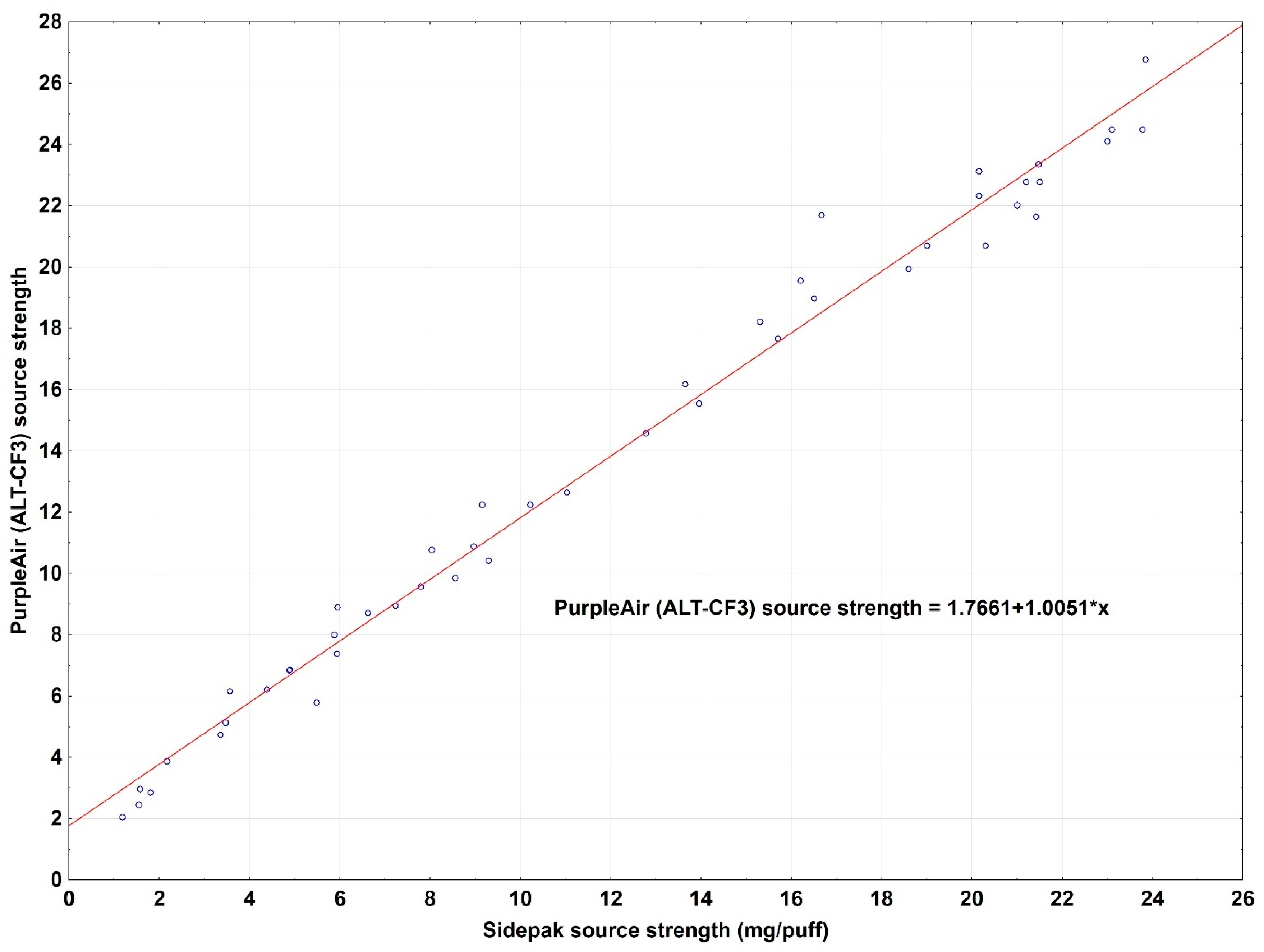
Calibration of PurpleAir Monitors 1 and 2

Prior to the start of the present study, two of the PurpleAir monitors used were calibrated against three research-grade optical particle counters (TSI Model 510 Sidepaks equipped with PM_2.5 cutpoint inlets) [27]. The particle source was aerosol produced from a single puff of marijuana smoke from a vaping pen. The Sidepaks were part of a group of six Sidepaks, which were in turn calibrated against gravimetric samplers sampling from the same indoor source [28]. Over an eight-month period, 47 experiments, each lasting 6–10 h, were carried out in a dedicated 30 m³ room of a home in Santa Rosa, CA, USA. The experiments plotted the decay of the particle concentration. Following initial mixing, the decay becomes linear (on a logarithmic scale) for a period of well-mixed concentrations. The slope is given by the sum of the air change rate a and the deposition rate k. The air exchange rate was measured by releasing a puff of carbon monoxide and tracking its decay using a Langan CO monitor T15. The regression line fitted to the decay curve can then be followed back to the beginning of the experiment to estimate the total mass released (in mg/puff), using a method developed in [29]. From the gravimetric experiments, the Sidepaks were determined to have a calibration factor (CF) of 0.44 (SE 0.03) [28]. The two PurpleAir monitors (numbers 1 and 2 with four independent Plantower sensors 1a, 1b, 2a, and 2b) were determined to have a calibration factor of 3.24, midway between the calibration factors of 3.0 and 3.4 found in various studies of outdoor air [4,19,20,28]. A linear least-squares regression of the PurpleAir monitors against the SidePaks resulted in a slope of 1.00 and an R² of 98.6% (Figure 3).

Two sites provided data using both the Plantower CF_1 and pm2.5 alt algorithms. At the Santa Rosa site where monitors 1 and 2 were calibrated, data were collected for one year (2021) using four monitors (eight Plantower sensors). Three PA-II monitors were collocated indoors in the same 30 m³ room where monitors 1 and 2 were calibrated. They were placed 1.5 m high with the intake unobstructed. One monitor was outside at a height of 2 m and at 1 m distance from the house. The monitors collected data every two minutes, and the data were averaged over 10 min periods. In 2022, two new PurpleAir Flex monitors with two Plantower PMS 6003 sensors each were added to the four existing monitors with the Plantower PMS 5003 sensors. Therefore, a second data collection period was selected for the Santa Rosa site running from 1 January 2023 to 13 July 2023.

At the Redwood City site, the data were collected by two collocated PA-II monitors at 1 m height in a 43 m³ room. One PA-II monitor was located outdoors. Two data periods were selected from this site. The first runs from 29 April 2021 to 31 October 2022. The second runs from 22 September 2022 to 23 June 2023.

In summary, four datasets from two locations were analyzed for this study (

Table 4. Datasets analyzed in this study.

Site	Year	Start Date	End Date	N obs
Santa Rosa	2021	1 January 2021	31 December 2021	52,400
Santa Rosa	2023	1 January 2023	13 July 2023	24,700
Redwood City	2021–2022	29 April 2021	31 October 2022	78,900
Redwood City	2022–2023	22 September 2022	23 June 2023	39,900

). Ultimately, 18 independent Plantower sensors were included.

3. Results

3.1. Santa Rosa Site

3.1.1. Santa Rosa 2021 Dataset

Monitors 1–4 were used throughout the full year 2021 in Santa Rosa. Since monitors 1 and 2 were calibrated against the SidePak earlier, they were considered reference monitors for this study. Monitor 3 (sensors 3a and 3b) monitored outdoor air. Monitor 4 was collocated indoors with monitors 1 and 2, so the 4a and 4b sensors estimates of PM_2.5 for the alt CF3.4 algorithm were compared with the mean values of monitors 1 and 2 (

Table 5. Comparison of collocated sensors 4a and 4b to the calibrated monitors 1 and 2.

	Valid N	Mean	Std. Err.	Median	Upper Quartile
mean calibrated monitors (1a, 1b, 2a, 2b)	48,073	2.95	0.029	1.60	3.14
4a pm2.5 alt CF3.4	52,435	2.94	0.039	1.37	2.80
4b pm2.5 alt CF3.4	52,435	3.09	0.042	1.36	2.91

).

For this year of 2021, the model was tested against the observed CF_1 PM_2.5 estimates for each of the eight sensors. The individual estimates of a–d are found in

Table 6. Estimates of a, c, and d for individual best-fit models of CF_1 PM_2.5 during 2021.

Sensor	N	a	c	d
1a	52,468	0.004127	0.093125	−0.84448
1b	52,468	0.003926	0.111286	−0.97701
2a	51,102	0.00379	0.12145	−1.08068
2b	51,102	0.00446	0.09843	−1.4993
3a	52,468	0.003148	0.103468	−0.78551
3b	52,468	0.003901	0.111096	−0.99718
4a	52,468	0.00476	0.08175	−1.06733
4b	52,468	0.003461	0.12012	−0.9171
mean		0.003947	0.105091	−1.02107
SD		0.000515	0.013643	0.218565
SE		0.000182	0.004824	0.077274
RSD		0.046158	0.045899	−0.07568
RSE		4.60%	4.59%	7.57%

. The mean of those estimates (highlighted row in Table 6) is the general model to be tested.

3.1.2. Santa Rosa 2023 Dataset

With the addition of the two Flex monitors in late 2022, all 12 of the Santa Rosa sensors were available for the 6-month period from 1 January 2023 to 13 July 2023. Mean PM_2.5 values for the three monitors 4–6 were compared to the calibrated monitors 1 and 2 (

Table 7. Comparison of collocated monitors 4–6 to the calibrated monitors 1 and 2 in 2023 data from the Santa Rosa site.

Sensor ID	Valid N	Mean	Std. Err.	Lower Quartile	Median	Upper Quartile
1a, 1b, 2a, 2b	24,727	1.01	0.010	0.32	0.61	1.17
4a	24,727	1.07	0.011	0.30	0.61	1.22
4b	24,727	1.16	0.012	0.33	0.64	1.26
5a	24,725	1.06	0.012	0.29	0.57	1.15
5b	24,725	1.15	0.013	0.31	0.62	1.24
6a	24,725	1.17	0.013	0.31	0.62	1.30
6b	24,725	1.07	0.012	0.30	0.59	1.18

). (Monitor 3 was outdoors, so sensors 3a and 3b could not be compared to the calibrated monitors 1 and 2.)

For the 2023 data, the model was tested against the observed CF_1 PM_2.5 estimates for each of the 12 sensors to determine the parameters a, c, and d for the individual best-fit models (

Table 8. Individual best-fit models of CF_1 for 12 sensors. The general model is calculated as the mean values of a, c, and d.

Sensor	N	a	c	d
1a	39,011	0.004109	0.092604	−0.614406
1b	39,011	0.003677	0.10811	−0.685727
2a	39,010	0.00447	0.096386	−0.76239
2b	39,010	0.00433	0.078342	−0.959499
3a	39,011	0.00382	0.095303	−0.678204
3b	39,008	0.003972	0.0986	−0.728282
4a	39,001	0.004565	0.079921	−0.92565
4b	39,001	0.004467	0.097416	−0.848253
5a	39,001	0.003897	0.097416	−0.848253
5b	39,001	0.003543	0.106866	−0.612662
6a	38,992	0.002672	0.123556	−0.775122
6b	38,992	0.003937	0.10173	−0.64114
mean		0.003955	0.098021	−0.75663233
SD		0.00052	0.012065	0.11799929
SE		0.00015	0.003483	0.03406346
RSD		0.131586	0.123084	−0.15595327
RSE		0.037986	0.035531	−0.04501983
RSE (%)		3.8%	3.6%	4.5%

). The mean of those estimates is the general model to be tested.

PM2.5 estimates from the best-fit individual models and the general model were regressed on observed CF_1 PM_2.5. Results are provided for the 12 tested sensors in Santa Rosa in 2023 (

Table 9. Regression results (intercept, slope, R²) for the individual models and the general model on observed values of CF_1 PM_2.5 from the period 1 January 2023 to 7 January 2023 at the Santa Rosa site.

		Individual Best-Fit Models			General Model
Sensor	N	Intercept	Slope	R2	Intercept	Slope	R2
1a	27,629	0.0115	0.9893	0.9894	−0.134	0.9944	0.9893
1b	27,629	0.0138	0.9877	0.9857	−0.0527	0.9747	0.9854
2a	27,628	0.0149	0.9887	0.9859	−0.018	0.9836	0.9857
2b	27,628	0.0342	0.9612	0.9565	0.2918	1.0116	0.9552
4a	27,611	0.0174	0.9858	0.9853	−0.0386	1.017	0.9853
4b	27,611	0.0111	0.9927	0.9906	0.1851	1.026	0.9919
3OUT a	27,611	0.0184	0.9925	0.9926	0.0491	0.9408	0.9931
3OUT b	27,611	0.0237	0.9932	0.9932	0.0491	0.9408	0.9931
5A	24,723	0.0095	0.9905	0.9905	−0.1325	1.004	0.9905
5b	24,723	0.0133	0.9883	0.9883	−0.1175	0.9925	0.9875
6a	24,723	0.0329	0.9858	0.9858	−0.1124	0.9727	0.9897
6b	24,723	0.0107	0.9898	0.9897	0.1864	1.0035	0.9798
mean		0.0176	0.9871	0.9861	0.0130	0.9885	0.9855
SD		0.0084	0.0085	0.0097	0.1425	0.0274	0.0103
SE		0.00243	0.00246	0.00280	0.04115	0.00792	0.00297
RSD		0.4781	0.0086	0.0099	10.9787	0.0278	0.0105
RSE		0.1380	0.0025	0.0028	3.1693	0.0080	0.0030
RSE (%)		13.8%	0.3%	0.3%	317.0%	0.8%	0.3%

). The individual models had a mean intercept of 0.01 µg/m³, a mean slope of 0.997, and a mean R² of 0.997. The general models had similar mean values, but a wider range of individual values. However, no general model failed to meet the EPA guidelines of 5 µg/m³ for the intercept (range: −0.2 to +0.4 µg/m³) and between 0.9 and 1.1 for the slope (range: 0.93 to 1.08) [17].

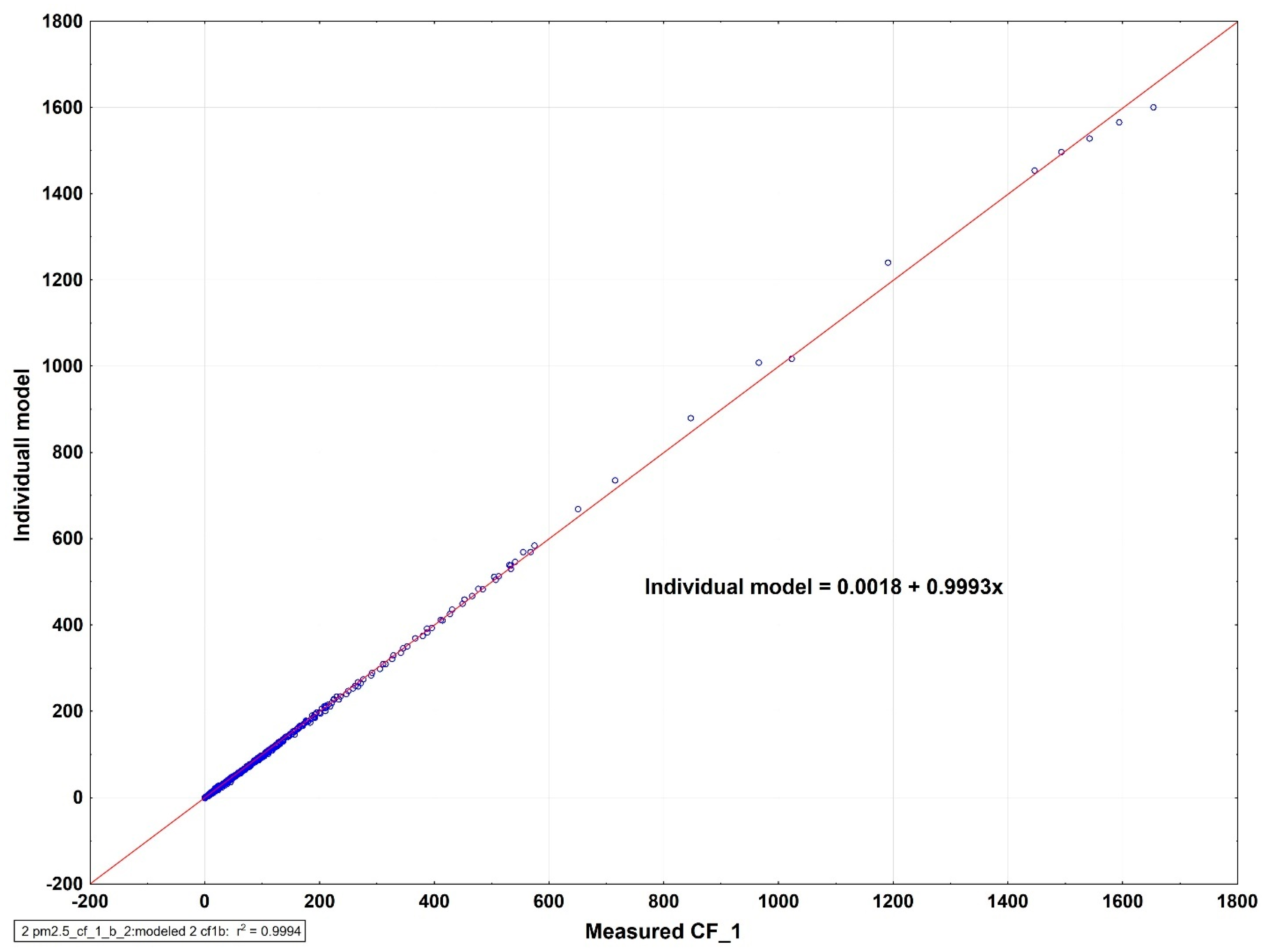
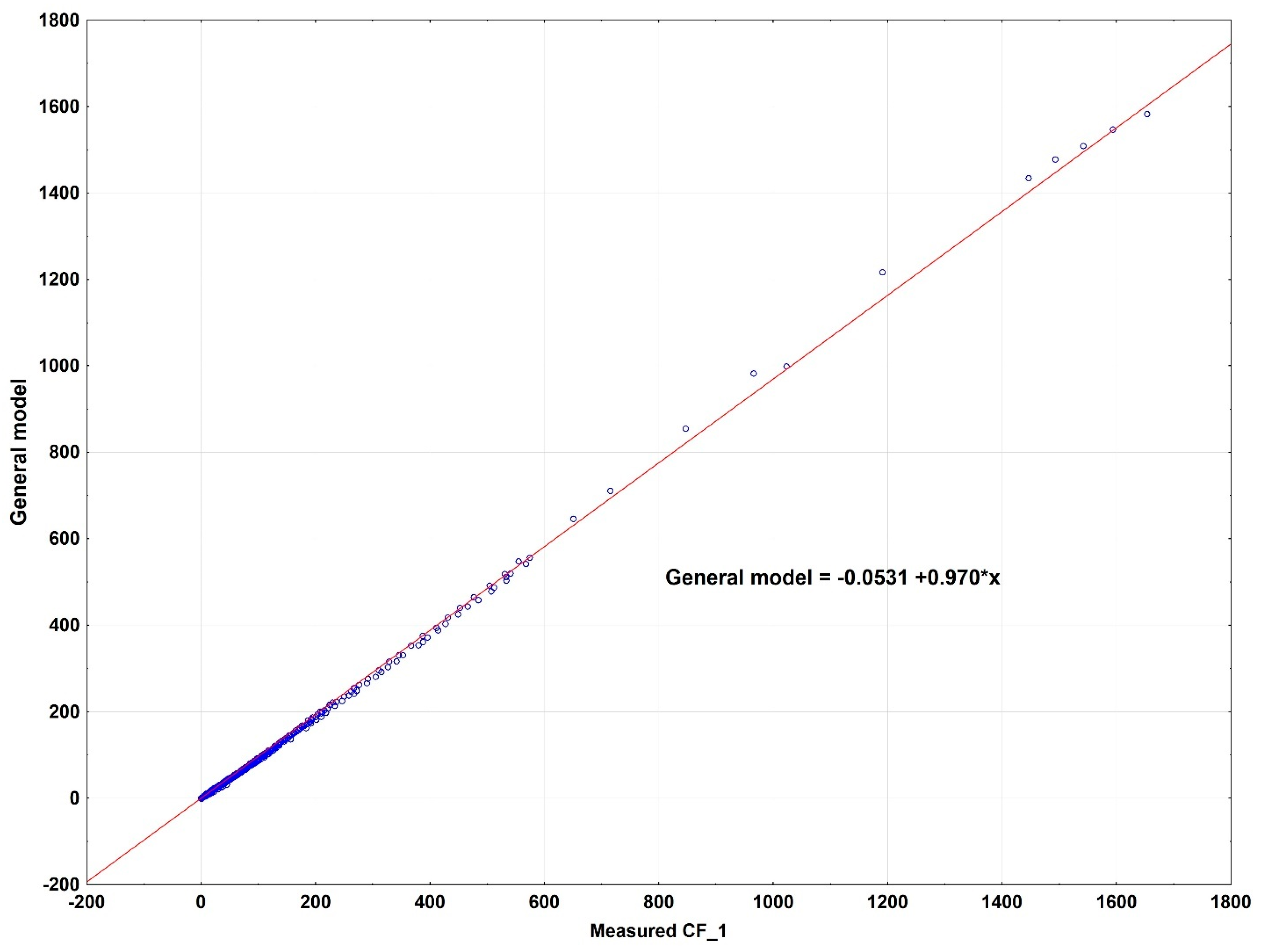
Examples of an individual best-fit model and a general model for the same sensor taken from the 9-month Santa Rosa data are provided in Figure 4 and Figure 5. Note the extremely close approach to a zero intercept and slope of 1.00 for the individual model. The general model has an intercept of −0.053 µg/m^3v and a slope of 0.97, but these are still very good results.

3.2. Redwood City

3.2.1. Redwood City 2021–2022 Dataset

For this 17-month dataset, all individual models approached the origin closely (0.006 to 0.048 µg/m³). Their slopes and R² values were above 0.99 in five of six cases. The general model also meets requirements for a good fit of a model to observed concentrations, with all intercepts less than 1 µg/m³ and all slopes between 0.95 and 1.065.

The results for the individual and general models may be found in the Supplementary Materials Section S1.3, Tables S1–S3.

3.2.2. Redwood City 2023 Dataset

For this 9-month dataset, the best estimates for a, c, and d are summarized in

Table 10. Best-fit estimates for parameters a, c, and d and regression results (intercept, slope, R²) for the individual models on observed values of CF_1 PM_2.5 from the period 22 September 2023 to 7 December 23 at the Redwood City site.

Sensor	a	c	d
7a	0.004836	0.085754	−0.823199
7b	0.004786	0.088221	−0.737484
8a	0.004441	0.091017	−0.776271
8b	0.003503	0.109911	−0.825874
9a OUT	0.00449	0.08056	−1.61195
9b OUT	0.00487	0.08143	−1.05379
mean	0.004488	0.089482	−0.971428
SD	0.000515	0.010767	0.332573536
SE	0.00021	0.004396	0.135772578
RSD	0.115	0.120	−0.342
RSE	0.047	0.049	−0.140
RSE (%)	4.7%	4.9%	14%

.

For the Redwood City site, the regressions of the individual models on observed CF_1 PM_2.5 all had intercepts below 0.2 µg/m³ and slopes >0.96 (

Table 11. Regression parameters (intercept, slope, r2) for the 2023 data from Redwood city.

Sensor	Individual Models			General Model
	Intercept	Slope	R2	Intercept	Slope	R2
7a	0.0114	0.9949	0.9949	−0.1413	0.9932	0.9995
7b	0.0133	0.995	0.9953	−0.1942	0.9502	0.9993
8a	0.0266	0.9905	0.9923	−0.04	0.994	0.9856
8b	0.1107	0.962	0.9611	0.0513	0.9892	0.9907
9a OUT	0.0568	0.991	0.991	0.7474	1.0646	0.9967
9b OUT	0.0202	0.9972	0.9972	−0.3219	1.0242	0.9979
mean	0.039833	0.988433	0.988633	0.016883	1.002567	0.99495
SD	0.038427	0.013201	0.013669	0.380112	0.038466	0.005601
SE	0.015688	0.005389	0.00558	0.15518	0.015704	0.002287
RSD	0.965	0.013	0.014	22.514	0.038	0.006
RSE	0.394	0.005	0.006	9.191	0.016	0.002
RSE (%)	39.0%	0.5%	0.6%	919%	1.6%	0.2%

). The general model performed well, with intercepts between −0.32 and +0.74 µg/m³ and slopes between 0.95 and 1.06. Thus, all models met the EPA requirement for an intercept absolute value less than 5 µg/m³ and a slope between 0.9 and 1.1.

Our second main objective is to compare the two algorithms cf_1 and pm2.5 alt for precision, accuracy, and limit of detection.

3.3. Precision

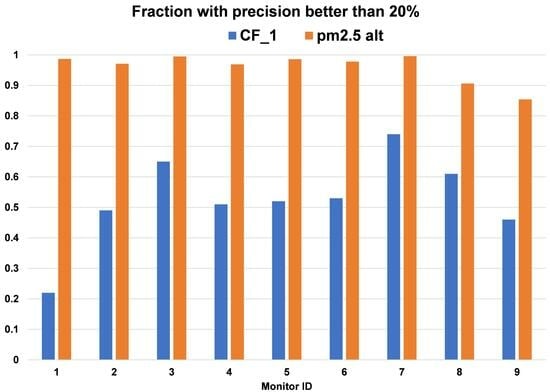
The precision of the CF_1 and pm2.5 alt algorithms is calculated by comparing the A and B sensors within a PA-II or Flex monitor. We have calculated precision by abs(A − B)/(A + B), although some prefer to use the coefficient of variation (CV) or relative standard deviation (RSD). The CV and RSD are equal to sqrt(2) times the precision as defined above. A reasonable choice for an upper limit on precision would be, say, 20% using the definition above, which corresponds to a CV or RSD of 28%. For each of the nine monitors during the 6-month 2023 period in both the Santa Rosa and Redwood City locations, the number of measurements meeting the precision standard of 20% is provided for both the CF_1 and pm2.5 alt algorithms (

Table 12. Comparison of the number of observations lost for the two algorithms due to poor precision.

Monitor	Total N	CF_1		PM2.5 alt
		N with Adequate Precision	Fraction with Adequate Precision	N with Adequate Precision	Fraction with Adequate Precision
1	39,012	8527	0.22	38,489	0.987
2	39,011	19,008	0.49	37,895	0.971
3	38,993	25,308	0.65	38,789	0.995
4	39,012	19,892	0.51	37,795	0.969
5	39,002	20,098	0.52	38,446	0.986
6	39,002	20,716	0.53	38,128	0.978
7	38,290	28,280	0.74	38,128	0.996
8	38,896	23,595	0.61	35,252	0.906
9	38,290	17,439	0.46	32,689	0.854

). For the CF_1 algorithm, the fraction of observations meeting the standard ranges from 0.22 to 0.74; for the pm2.5 alt algorithm, the fraction ranges from 0.85 to 0.99.

The major loss of observations for the CF_1 algorithm shown in the above table is due in part to the many values of zero that occur. However, the zero values are not the only reason for the poor performance. Even considering only those observations with a precision meeting the standard, the mean and median precision estimates for the CF_1 algorithm are consistently worse than for the pm2.5 alt algorithm. Comparing the precision of the six Santa Rosa monitors in 2023 for the two algorithms CF_1 and pm2.5 alt, the upper limit of 0.2 is easily met by the pm2.5 alt algorithm, whereas no mean value for the CF_1 algorithm was able to meet the 0.2 upper limit (

Table 13. Measured precision using the CF_1 and pm2.5 alt algorithms for six PA-II monitors in Santa Rosa during 2023.

	Valid N	Mean	Median	Upper Quartile	90th Percentile
1 precision pm2.5 alt	39,012	0.050	0.039	0.067	0.11
2 precision pm2.5 alt	39,011	0.059	0.043	0.081	0.13
4 precision pm2.5 alt	39,012	0.062	0.047	0.084	0.13
3 OUT precision pm2.5 alt	38,993	0.048	0.038	0.067	0.10
5 precision pm2.5 alt	39,002	0.053	0.040	0.071	0.11
6 precision pm2.5 alt	39,002	0.053	0.037	0.068	0.11
1 precision CF_1	32,650	0.53	0.51	0.94	1.00
2 precision CF_1	29,103	0.26	0.11	0.32	1.00
4 precision CF_1	30,282	0.26	0.11	0.32	1.00
3 OUT precision CF_1	36,584	0.21	0.13	0.23	0.45
5 precision CF_1	29,618	0.24	0.09	0.29	1.00
6 precision CF_1	30,060	0.23	0.08	0.27	1.00

).

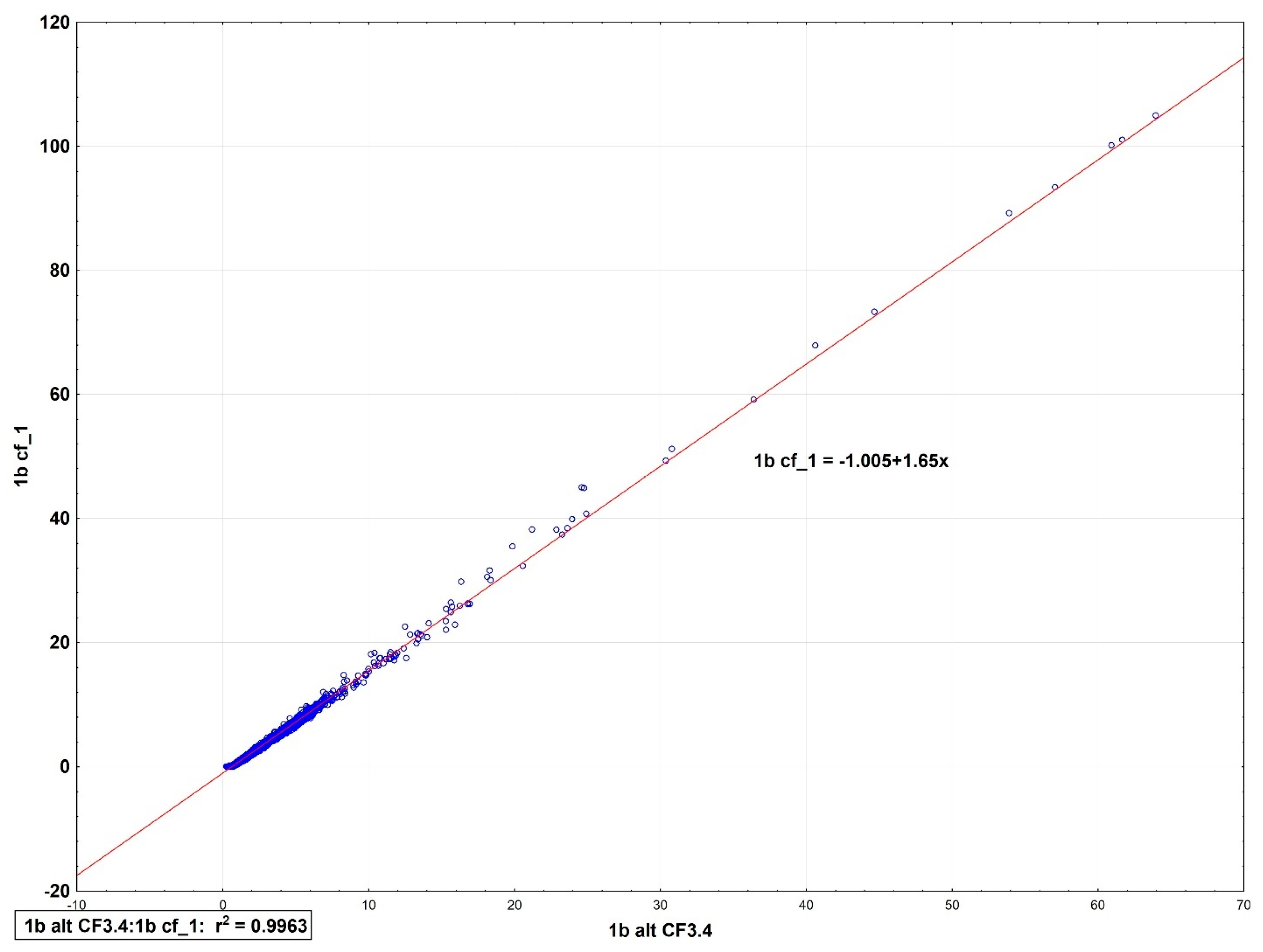
3.4. Accuracy

Since monitors 1 and 2 were calibrated by collocation with three research-grade TSI Sidepaks Model 510, which had themselves been calibrated against gravimetric monitors, we estimate the accuracy of the CF_1 algorithm using the average of these two monitors (four sensors) as the reference. Regressions of the CF_1 estimates against the alt CF3.4 estimates for sensors 1a, 1b, 2a and 2b resulted in slopes of 1.60, 1.65, 1.63, and 1.70, indicating overestimates by 60–70% for the CF_1 algorithm. Similar overestimates have also been noted by multiple investigators [3,9,10,12,13,14]. An example is shown from the most recent dataset from 1 January 2023 to 13 July 2023 (Figure 6).

Limit of Detection (LOD)

The LOD for the two algorithms was calculated using a method introduced in [30]. The method involves identifying all cases with the mean/SD < 3 and searching for their appearance in “batches” of 100 or so samples ordered by concentration. If, beyond a certain concentration, there are no cases with five or more such values appearing in each 100-sample batch, then the LOD has about a 95% probability of being that concentration. The LOD is of particular interest for indoor studies since indoor concentrations are often quite low. For the five collocated indoor PA-II and Flex monitors in the most recent 2023 data from Santa Rosa, the LOD was 0.106 µg/m³ for the pm2.5 alt algorithm and 1.22 µg/m³ for the CF_1 algorithm. Although both values seem fairly small, because of the low concentrations in general, only 29% of the 39,014 measurements were above the CF_1 LOD, compared to 99% above the LOD for the pm2.5_alt algorithm.

4. Discussion

In summary, four new datasets with about 200,000 additional observations were employed to test the basic model of Equation (5) on 18 independent particle sensors (14 PMS 5003 sensors and 4 PMS 6003 sensors). The individual best-fit models performed superlatively well, with intercepts mostly within ±0.1 µg/m³ and slopes mostly close to 0.99. Even the general models were well within the guidelines of a successful model, with intercept absolute values always less than |1| µg/m3 and slopes between 0.95 and 1.06. The four new general models all had estimates for the a and c parameters generally within ± 10% (

Table 14. Comparison of general model parameters for four new datasets with the original finding in [26].

Site	Year	N obs	a	c	d
Santa Rosa 1	2020	134,800	0.0042	0.10	−1.1
Redwood City	2021–2022	78,900	0.0045	0.09	−1.0
Santa Rosa	2021	52,400	0.0040	0.11	−1.0
Redwood City	2022–2023	39,900	0.0045	0.09	−1.0
Santa Rosa	2023	24,700	0.0040	0.10	−0.8

¹ From [26].

). Because of the small value for the additive constant d, the percentage difference was larger, at about 10–20%.

A measure of the fit of a model to observations is the Mean Absolute Error (MAE). MAE results were calculated for the individual models and for the general model fits for the eight sensors in the Santa Rosa site for the 1 January 2023 to 13 July 2023 dataset. For individual sensors, MAEs ranged from 0.17 to 0.42 µg/m³. For the general models, the range was only slightly larger, from 0.20 to 0.52 µg/m³. For the four Flex sensors, the range was from 0.21 to 0.30 for the individual models and 0.23–0.34 for the general models. For the Redwood City 2023 data, the MAEs for the six sensors 7a to 9b ranged between 0.13 and 0.34 µg/m³ for the individual models and between 0.21 and 0.38 µg/m³ for the general model, with the exception of an MAE value of 1.24 µg/m³ for sensor 9a, which had a constant offset of 1.75 µg/m³. Once this offset was subtracted from every measurement, the agreement with sensor 9b was quite good. This was the only case of a bias encountered among the 18 sensors tested.

These findings provide support for the original hypothesis in [1] that the CF_1 algorithm has the form shown in Equation (5), in which the numbers of particles N1 and N2 in the two smallest datasets are combined and multiplied by a single parameter. There is also support for the hypothesis that there is an additional additive component d of order −1 µg/m³. When this value is used in both the individual and general models, the number of negative values in the models almost exactly matches the number of zeros reported by the CF_1 algorithm. This observation suggests a reason for the otherwise mysterious appearance of multiple zeros in CF_1 estimates when in fact the number of particles in N1 is never zero.

Precision of the CF_1 algorithm was consistently worse than that for the pm2.5 alt algorithm, with 26–78% of values unable to meet the standard of 20%. For the pm2.5 alt algorithm, 90–99% of values met the standard for eight of the nine monitors, and even the ninth monitor lost only 15% of the values compared to 54% for the Cf_1 algorithm.

Accuracy, as found by regressing CF_1 values on the average of the four calibrated sensors, ranged between 60 and 70% overestimates, agreeing with multiple other studies.

The limit of detection for the CF_1 algorithm, although not obviously high at 1.22 µg/m³, was more than 10 times higher than the LOD of 0.11 for the pm2.5 alt method, resulting in a large percentage of values (71%) below the LOD, compared to 1% for the pm25 alt algorithm.

Finally, we have provided in the Supplementary Materials a brief history of the development of health standards dating from the London fog of 1952 [31,32] and the development of aerosol instrumentation for workplace monitoring [33,34,35], which led ultimately to the development of today’s low-cost particle monitors [36,37].

5. Conclusions

We find first that the CF_ATM algorithm offered by Plantower has no physical basis and should not be used.

Secondly, we have confirmed the finding that the CF_1 algorithm has the form a(N1 + N2) + cN3 + d and have estimated values for a, c, and d within about 10–20% tolerance. The finding that the additive component d is a negative value on the order of −1 µg/m³ may explain the large number of zeros often reported by the CF_1 algorithm—they are due to negative concentrations predicted by the CF_1 algorithm and therefore are set to zero.

Thirdly, the bias of the CF_1 algorithm, compared to calibrated monitors using the pm2.5 alt algorithm, is on the order of 60–70% overestimates of PM_2.5, a result similar to those of many investigators. Precision, particularly for the low PM_2.5 concentrations commonly found for indoor air, is poor, resulting in loss of 71% of observations in the most recent 2023 dataset analyzed. The CF_1 LOD for this set of observations in 2023 was more than 10 times the LOD for the pm2.5 alt algorithm, resulting in only 29% of observations exceeding the LOD, compared to 99% for the pm2.5 alt algorithm.