Visual Static Hand Gesture Recognition Using Convolutional Neural Network

Abstract

Hand gestures are an essential part of human-to-human communication and interaction and, therefore, of technical applications. The aim is increasingly to achieve interaction between humans and computers that is as natural as possible, for example, by means of natural language or hand gestures. In the context of human-machine interaction research, these methods are consequently being explored more and more. However, the realization of natural communication between humans and computers is a major challenge. In the field of hand gesture recognition, research approaches are being pursued that use additional hardware, such as special gloves, to classify gestures with high accuracy. Recently, deep learning techniques using artificial neural networks have been increasingly proposed for the problem of gesture recognition without using such tools. In this context, we explore the approach of convolutional neural network (CNN) in detail for the task of hand gesture recognition. CNN is a deep neural network that can be used in the fields of visual object processing and classification. The goal of this work is to recognize ten types of static hand gestures in front of complex backgrounds and different hand sizes based on raw images without the use of extra hardware. We achieved good results with a CNN network architecture consisting of seven layers. Through data augmentation and skin segmentation, a significant increase in the model’s accuracy was achieved. On public benchmarks, two challenging datasets have been classified almost perfectly, with testing accuracies of 96.5% and 96.57%.

1. Introduction

In order to communicate with computers in more effective and natural ways, researchers have experimented with various methods for more than half of the last century. Over time, human interaction was made mainly via a keyboard and mouse. Most of the time, we interact with computers using our fingers and eyes, but other body parts, including our legs, arms, and mouth, are underutilized or never used at all. This is inconvenient since it is like composing emails with just one finger. Standard image processing methods do not produce excellent results, so machine learning is required for gesture detection to reach its full potential. Gestures are meaningful, expressive body motions that involve physical movements of the body, hands, arms, head, face, and fingers. Gesture recognition is the process that seeks to identify gestures and translate them into commands that can facilitate effective communication between humans and computers. Hand gestures are either dynamic or static. Implicit hand gestures and postural behavior are considered for the recognition of emotional states [1,2]. However, this paper is meant to focus more on the recognition of static, explicit hand gestures.

At present, there are some problems in visual gesture recognition, such as accuracy, real-time, and poor robustness. Although there are many methods of gesture recognition, vision-based gesture recognition still faces many serious problems in practice. It is mainly reflected in a low recognition rate, poor robustness, insensitivity in real-time, and poor practicability. Gesture recognition should bring great results no matter the background; it should work whether you are in the car, at home, or walking down the street. Using CNN helps overcome the problem of identifying gestures in complex backgrounds with very high accuracy.

Advancements in CNN and the recently emerged deep learning techniques avoid the need for deriving complex handcrafted feature descriptors from images, so they outweigh the classical approach to hand gesture recognition [3,4,5,6]. By learning the high-level abstractions in images, CNN automates the feature extraction process and uses hierarchical architecture to capture the most discriminative feature values [7,8].

In ref. [9], Gao et al. proposed a parallel CNN model that used RGB and depth images as input. Parallel CNN consists of two CNNs, namely depth-CNN and RGB-CNN, where one takes a depth image as input while the other takes an RGB image as input. A prediction probability was weighted on the last layer of each CNN output and concatenated to have the input to a softmax classifier layer. The dataset used contains a total of 24 hand gestures, representing the 24 letters (except J and Z, because J and Z are dynamic hand gestures). Each gesture contains 5000 sample images, which are 2500 RGB images and 2500 depth images, completed by 5 people in different backgrounds with different illumination. So there are a total of 120,000 pictures, which are 60,000 RGB images and 60,000 depth images. The model accuracy has reached 93.3% for American Sign Language (ASL). The advantage of this approach is its ability to capture both appearance and depth information.

In ref. [10], Oliveira et al. proposed CNN with four convolutional layers, with a max-pooling layer affixed to each convolutional layer, followed by a fully connected layer and a softmax classifier. The proposed CNN was able to attain 99% for Irish Sign Language (ISL). The dataset was collected by filming human subjects performing ISL hand shapes and movements and then extracting frames from the videos. This produced a total of 52,688 images for the 23 common hand- shapes from ISL. The very high accuracy can be explained by the simple image black backgrounds, which make it so easy and unchallenging to identify images and gestures. However, this method may struggle when applied to real-world scenarios with complex backgrounds and lighting variations, which is a disadvantage. In the proposed method, we will solve that by working on datasets with complex backgounds. Arenas et al. [11] derived a CNN architecture from a directed acyclic graph (DAG) structure (DAG-CNN). A self-constructed dataset was used to experiment with the model on. The dataset consists of 10 gestures for controlling the robotic arm, and model accuracy was 84.5%. However, the model’s performance may vary when applied to different gesture recognition tasks.

Using fully connected layers of a pre-trained artificial neural network (AlexNet), Sahoo et al. [12] proposed a deep CNN feature-based static hand gesture recognition system. This system reduces redundant features using principal component analysis after deep features are extracted using fully connected layers of AlexNet (PCA). An SVM was then used as a classifier to categorize the poses of hand motions. The dataset was developed from five subjects with 36 gesture poses (10 ASL digits and 26 ASL alphabets). The dataset has variations in illumination in five different directions, such as left, right, top, bottom, and diffuse. The gesture poses are performed with variation in hand rotation, scale, and articulation. The American Sign Language dataset was used to test the system’s performance on 36 gesture postures, and the average accuracy score was 87.83%. Wadhawan et al. [13] proposed a generic CNN architecture for static sign language recognition. The dataset used comprises 35,000 images, which include 350 images for each of the static signs. There are 100 distinct sign classes that include 23 alphabets of English, 0–10 digits, and 67 commonly used words (e.g., bowl, water, stand, hand, fever, etc.). The network had an accuracy of 98.85% on the Indian sign language dataset. However, this approach may face challenges when applied to complex backgrounds, as the dataset consists of images captured on a simple white background that can be identified as relatively unchallenging.

For the purpose of assessing human behavior in the context of classroom learning and instruction with two teachers, Wang et al. [14] introduced a recognition model of hand gestures based on CNN. The analysis of the teacher’s nonverbal behaviors that improve the learning results of learners and attract their attention is achieved by exploiting the recognized instructors’ hand gestures. A non-linear neural network with four convolutional layers is used in this model to extract the features of hand gesture images. For achieving robust recognition, three convolution layers of CNN are designed. A dataset of 38,425 infrared hand gesture images extracted from 100 short infrared videos is used to test and evaluate the model. The model has reached an accuracy of more than 92%. The model has the advantage of using a dataset that gives good results. Nevertheless, the images are also simple, with simple infrared backgrounds.

In ref. [15], Zuocai Wang et al. suggested a method for identifying hand gestures through the use of particle filtering. By implementing this filtering technique on hand gesture images with identical backgrounds, the researchers achieved an accuracy of 90.6%. However, it has the disadvantage that performance may degrade when backgrounds are not stationary. In ref. [16], Suguna and Neethu utilized shape features obtained from hand gesture images to categorize them into different classes. The extracted features were then taught and sorted into clusters using the k-means clustering algorithm. This approach offers simplicity but may struggle with complex hand gestures. In ref. [17], Marium et al. put forward a method for hand gesture recognition that involved the use of a convexity algorithm approach. The researchers tested this technique on hand gesture images with identical backgrounds and obtained an accuracy of 87.5%. However, the approach was limited by the fact that the algorithm worked best when the background of the hand gesture image was stationary.

In ref. [18], Ashfaq and Khurshid converted spatial domain-format hand gesture images into multi-class domain-format images using the Gabor filtering approach. They employed both Bayesian and Naive Bayes classifiers to categorize the test hand gesture images into different classes. The researchers found that the naive Bayes classifier produced higher levels of classification accuracy than the Bayesian classification methodology, owing to its straightforward architecture pattern. The data is acquired by a 7-megapixel camera. The dataset used has a total of ten hand gestures. For each hand gesture, there are 18 images, of which 5 are used for training and 13 for final testing. The model has an accuracy of 90%. In [19], Rahman and Afrin used an SVM classification approach in 2013 to categorize hand gesture images into various classes. The training set for the detection phase consisted of over 800 positive samples and 1500 negative image samples. The researchers achieved a sensitivity of 89.6%, a specificity of 79.9%, and an accuracy of 85.7%. However, the error rate was high in this method, and it was not suitable for fast-moving background and foreground object images.

In ref. [20,21], Authors utilized naive Bayes Classifier and SVM approaches for recognizing gestures, but these methods were unable to handle large training datasets and needed a large number of training samples. To overcome these limitations, the current study introduces a CNN classifier, which does not require a large number of training samples and has a low complexity level. In ref. [22], Rao et al. developed a hand gesture recognition system using a hidden Markov model. The authors constructed a Markov model for the foreground fingers in a hand gesture image. This model was used in both the training and testing of the binary classification approach, giving it an accuracy of 90.1%.

In ref. [23], the hand postures are classified using the shape, texture, and color features with an SVM classifier. The proposed system utilizes a Bayesian model of visual attention to generate a saliency map and to detect and identify the hand region, and they reported an accuracy of 94.36% on the NUS II dataset that we use in our research. In ref. [24], the authors proposed a CNN model with two convolutional layers, two max-pooling layers, and one last fully connected layer. Dropout and activation functions are optional. However, they reported better results using both of them. The best accuracy reported on the NUS-II dataset was 89.1% by adding the dropout and activation functions. In our research paper, we will compare our results with the ones in refs. [23,24] as they reported results on the same challenging dataset we use and they also use CNN.

In this research, we propose a CNN to recognize static hand gestures against complex backgrounds. The objective is to increase the accuracy of correctly identified gestures. Testing the accuracy of the model is achieved by comparing the true label of the image with the predicted label. The efficiency of deep learning in extracting and classifying high-level aspects of data has recently been the focus of existing research.

In summary, the contributions of this paper are adding the power of newly proposed preprocessing techniques in this research for the images using skin segmentation and data augmentation with the power of using CNN for classifying images. To the best of our knowledge, there has been no previous publication that has performed skin segmentation on the NUS II dataset using the same methodology we used. In addition, there is no paper that reported any results of combining both the CNN model and skin segmentation on a complex dataset such as the NUS II dataset, as we performed.

We compare our accuracy on the NUS II dataset to the one in refs. [23,24], as they both use different state-of-the-art methods on the same dataset. The accuracy of our proposed method has improved from the one in ref. [24], going from 89.1% to 96.5%, as the number of misclassified images has decreased from representing 10.9% of the test dataset to only 3.5%. We also compare our accuracy on the Marcel dataset to the one in refs. [24,25], as they also both use different state-of-the-art methods on the same dataset. The accuracy of our proposed method has improved from the one in ref. [24], going from 85.59% to 96.57%, as the number of misclassified images has decreased from representing 14.41% of the test dataset to only 3.43%.

In Section 2, the concepts of skin segmentation, data augmentation, cross-entropy loss function, and the structure of the newly proposed CNN are introduced. We also discuss the training details and analysis of different methods and tools used in different training experiments. In Section 3, we discuss the results of the proposed experiments. Finally, In Section 4 and Section 5, we discuss how the results can be interpreted from the previous state-of-the-art methods in refs. [23,24,25], how well they have improved, and our conclusion.

2. Materials and Methods

2.1. Introduction

In spite of the advances in image processing techniques and gesture recognition, an essential challenge is still unsolved: how can we recognize gestures in complex backgrounds without using hardware with a high level of accuracy? It turns out that using CNN helps us a lot to achieve that with very high accuracy by using the right dimensions for the CNN layers and choosing the best optimization techniques.

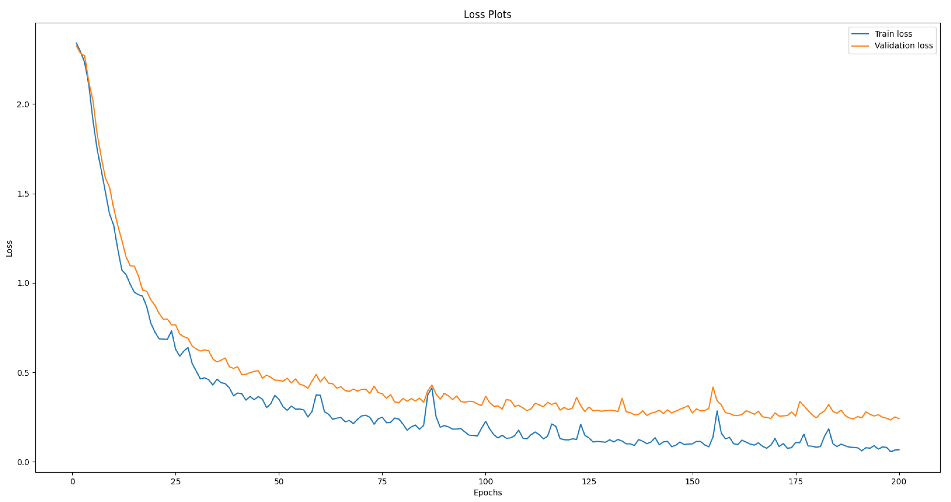
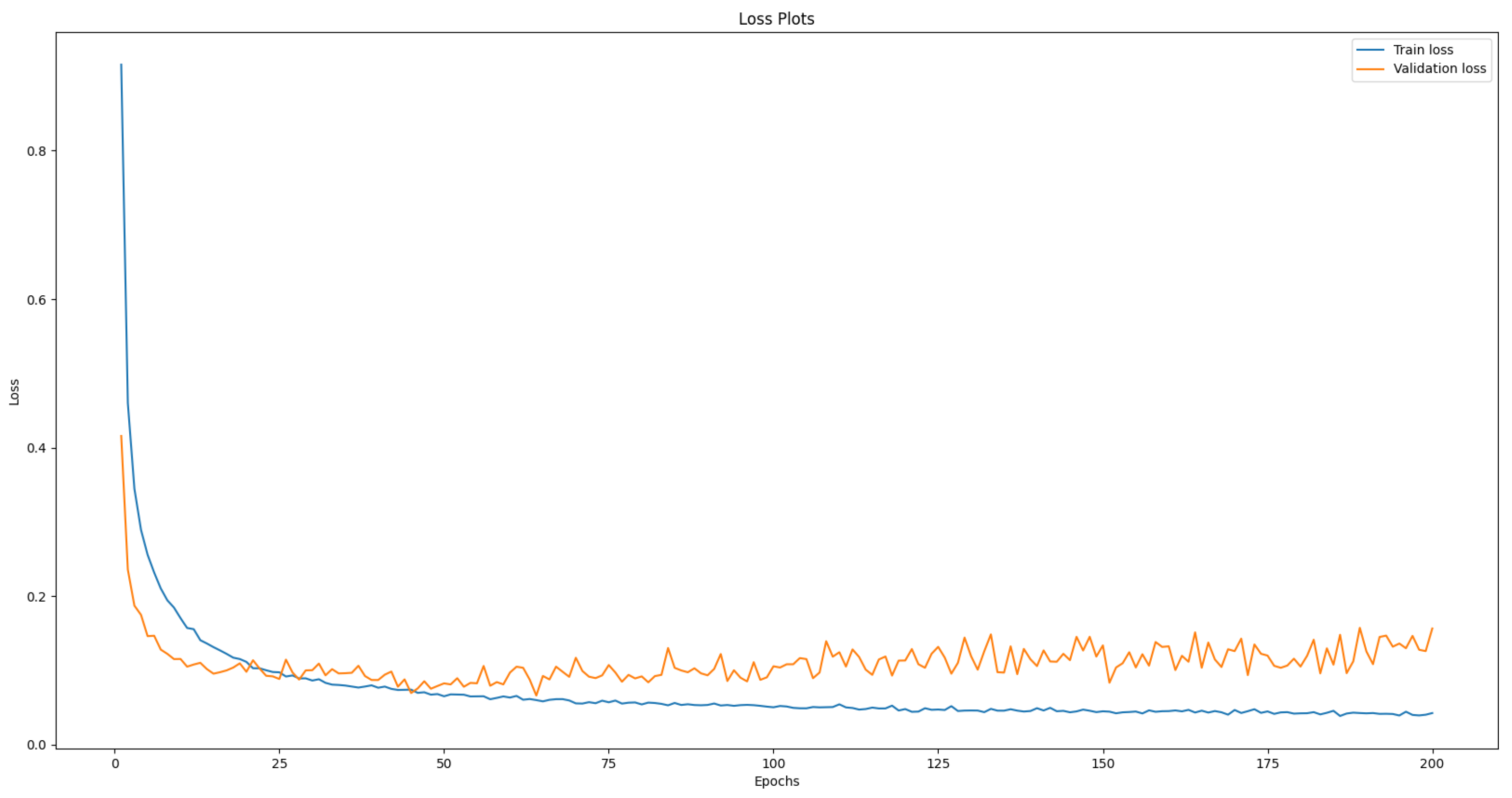
Identifying the right label for the test image is the optimization aim of our CNN model. We can achieve this by minimizing the loss function for the training and validation datasets to achieve as much accuracy as possible. To train the model, skin segmentation is used to reduce the data in the image and remove unwanted pixels that do not have skin HSV values. The challenge with this technique is that some pixels in the background already have skin colors, but it helps reduceing the data in the image and reduces the loss significantly.

Softmax is used to measure the predicted probabilities of each class by assigning them values between 0 and 1. As a consequence of using softmax, the cross-entropy loss function is used to measure the loss for the training dataset. Cross-entropy loss, or log loss, measures the performance of a classification model whose output is a probability value between 0 and 1. Cross-entropy loss increases as the predicted probability diverges from the actual label. Data augmentation is used to increase the dimensions of our training dataset, but validation and test datasets are not affected, and it has shown a significant increase in accuracy and decrease in the loss function as it helps in reducing overfitting and giving the model more data to train on.

2.2. Structure of the CNN

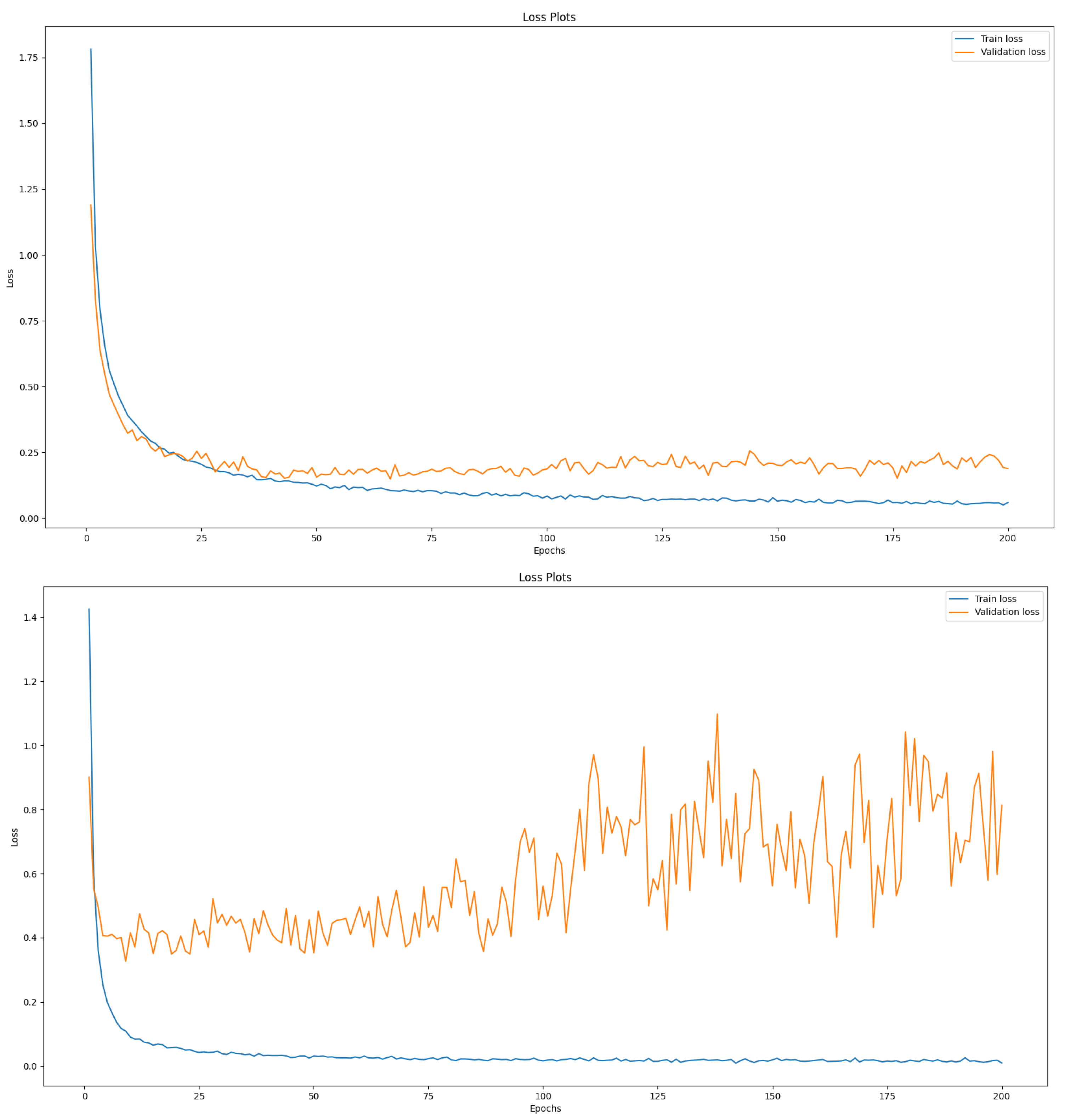
The motivation for proposing the chosen CNN architecture is the aim to leverage the hierarchical features of hand gestures, exploit translation invariance, reduce dimensionality, and efficiently extract discriminative features. The cascaded layers of convolutional and max-pooling operations in the architecture allow the network to progressively learn and extract increasingly complex features from the input images as a hierarchical feature extraction. The initial convolutional layer with 15 output maps captures low-level visual patterns, while subsequent layers with increasing output maps can learn more abstract and high-level features relevant to hand gesture recognition. This hierarchical feature extraction enables the network to effectively model the intricate details and variations present in hand gestures. The max-pooling layers in the architecture help reduce the spatial dimensions of the feature maps, resulting in a more compact representation of the learned features. By downsampling the feature maps, the max-pooling layers retain the most salient information while discarding less relevant or redundant details. This dimensionality reduction helps to mitigate the impact of background noise, variations in hand pose, and other sources of variability in hand gesture images, making the model more robust and efficient. We resize the input size of images to 32 × 32 to reduce overfitting. If we use a bigger size, the model will overfit, as we will show in the results of Section 3.6 by using image sizes of $64\times 64$ and showing the increase in the overfitting.

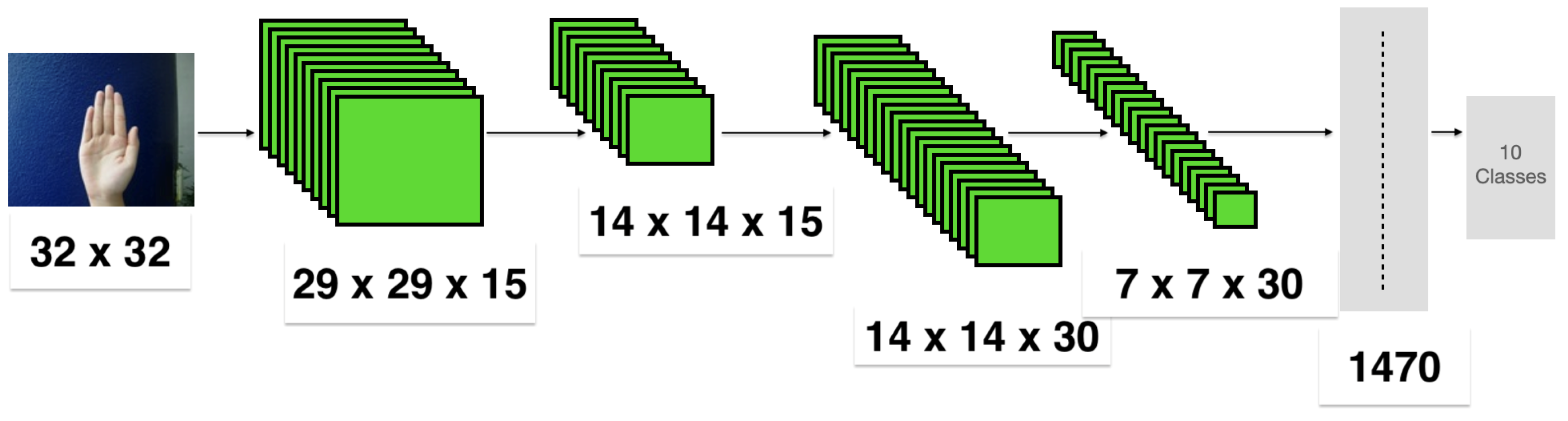
As shown in Figure 1, the CNN model consists of two convolutional layers, followed by a ReLU activation function for each one, and two pooling layers apart from the input and output layers. As shown in Figure 1, the input image of $32\times 32$ pixels is convolved with 15 filter maps of size $6\times 6$ to produce 15 output maps of $29\times 29$ in the first layer. These output maps are operated upon with a ReLU activation function. Downsampling of the output convolutional maps is completed with max-pooling of $2\times 2$ regions to yield 15 output maps of $14\times 14$ in layer 2. The 10 output maps of layer 2 are convolved with each of the 30 kernels of size $3\times 3$ to obtain 30 maps of size $14\times 14$. These maps are further downsampled by a factor of 2 by max-pooling to produce 30 output maps of size $7\times 7$ of layer 4. The output maps from layer 4 are concatenated to form a single vector during training and fed to the next layer, which is the fully connected layer. A dropout probability of 0.5 is used to reduce overfitting.

2.3. Skin Segmentation

The first technique we use to try to make the model learn better and increase its accuracy is skin segmentation, which will be used in the second experiment. Segmentation aims at partitioning areas in the image based on color, shape, and textures. It is useful in many computer vision applications. such as medical image analysis, object detection, and content-based image retrieval CBIR [26].

The skin segmentation technique is completed using the OpenCV python binary extension loader module. The segmentation is achieved by first converting the image from RGB to HSV color space to be able to extract the hue values for skin colors. In the OpenCV library in python, the measuring unit of hue values in the HSV (Hue, Saturation, Value) color space is typically 8-bit unsigned integers, ranging from 0 to 179. This means that hue values are quantized into discrete values, where each integer represents a specific hue bin or hue category. The 0 to 179 range is used to represent the full 360 degrees of hue values typically used in other systems, where each bin or category corresponds to a hue angle increment of approximately 2 degrees (360 degrees divided by 180 bins). This integer representation allows for efficient storage and processing of hue values in digital images and computer vision applications.

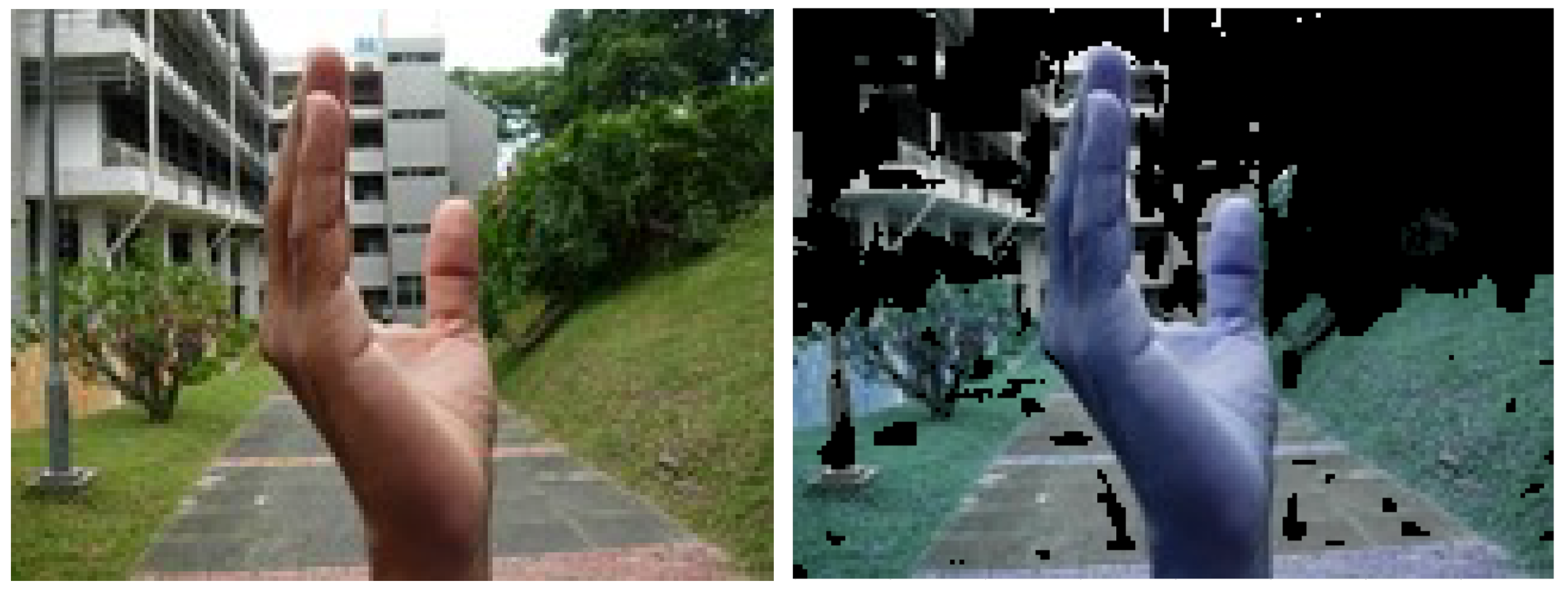
Hue values for skin colors are found to range from 0 to 38, which means they are ranging from 0 to 76 degrees in the normal HSV color space. The saturation and value (also known as brightness) are given a complete range from 0 to 255. This is completed to overcome the complex background, which has a wide range of brightness values that can be very dark or very bright. We only truncate the values for hue, which give us the true skin pixels, whatever the value of the saturation of light or brightness. Note also that images have a complex background, which includes skin-colored surfaces. Therefore, any skin-colored surface in the background is included in the image. Nevertheless, overall, it is better than the normal image, as there are a lot of unwanted pixels in the background that are removed, which makes us use only pixels that we can learn the most from during the training and validation phases.

2.4. Data Augmentation

Data augmentation is a very powerful technique for constructing better datasets. Many augmentations have been proposed, which can generally be classified as oversampling techniques. Deep learning models rely on big data generated from data augmentation to avoid overfitting. Artificially inflating datasets using methods of data augmentation achieves the benefit of big data in the limited data domain [27].

Data augmentation is used on the training data of two datasets used (NUS II and Marcel datasets) to increase the size of each by 10 times. The data augmentation is performed by randomly rotating each image by an angle that ranges from 20 degrees to the left to 20 degrees to the right.

2.5. Dropout

Dropout is a regularization technique that helps address the issue of overfitting in neural networks. During training, standard backpropagation learning can result in brittle co-adaptations that only work well on the training data and do not generalize to new, unseen data. By randomly dropping out or deactivating a fraction of hidden units during each training iteration, dropout disrupts these co-adaptations, making the presence of any particular hidden unit less reliable. This technique has been found to be effective in improving the performance of neural networks in various application domains, such as object classification, digit recognition, speech recognition, document classification, and computational biology data analysis [28]. In our proposed CNN, The dropout is added at the end of our model before the last fully connected layer to reduce the overfitting that is reaching the final layer and make the model generalize to new, unseen data.

2.6. Loss Function

The loss function that has been used is the logarithmic loss, log loss, or logistic loss. Each predicted class probability is compared with the actual class desired output of 0 or 1, and a score/loss is calculated that penalizes the probability based on how far it is from the actual expected value. The penalty is logarithmic in nature, yielding a large score for large differences close to 1 and a small score for small differences tending to 0.

Cross-entropy loss is used when adjusting model weights during training. The aim is to minimize the loss, i.e., the smaller the loss, the better the model. A perfect model has a cross-entropy loss of 0. Cross Entropy is defined as follows:

$$L=-\sum _1^n{p}_i\ast log\left(q_i\right)$$

(1)

Here, n is the number of classes, $p_i$ the true probability of the ith class in the target, and $q_i$ the softmax probability for the ith class.

Here, if we look at Equation (1), we can see that loss is calculated for each training example by calculating the negative natural logarithm for the output of the softmax function ($q_i$) multiplied by the true probability of the target, which is 0 or 1 ($p_i$). After calculating the loss for every training example, we sum all of them to get the training loss of the whole training dataset.

2.7. Training Details

All the experiments were completed on the Google colab CPU. Before training, the images are resized to 32 × 32. A batch size of 64 is used for the training set, and a batch size of 32 is used for both the validation set and the test set. Each image is resized into 32 × 32 and then enters the first convolution layer for the training phase. A learning rate of 0.001 is used with Adam optimizer as our optimization function.

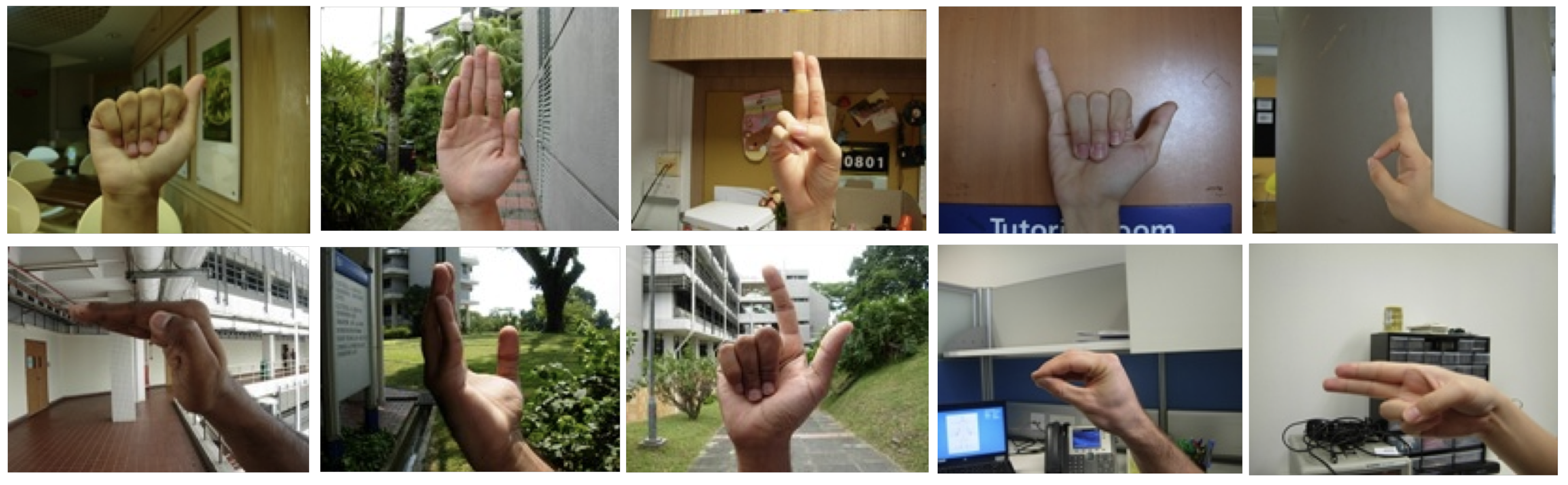
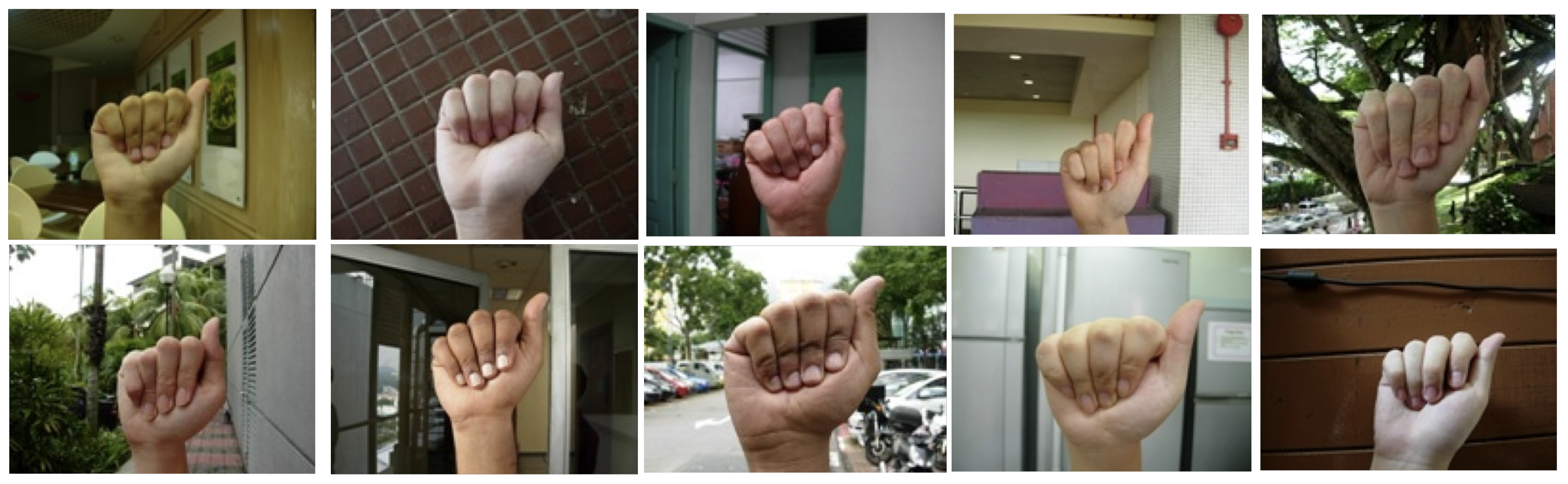
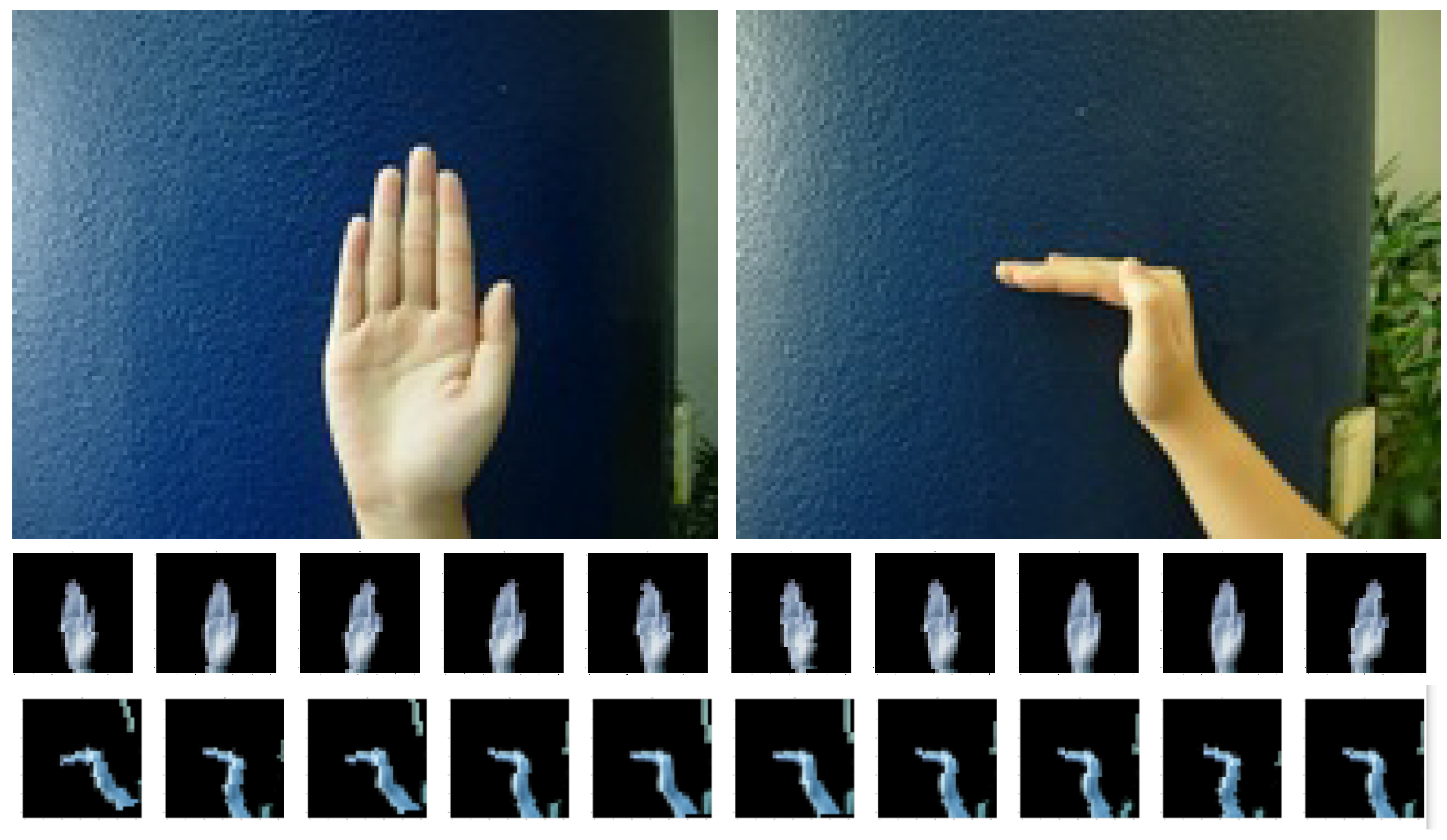
NUS II Dataset and Marcel datasets are the two dataset used for the training. NUS II dataset is a 10-class hand posture dataset, as shown in Figure 2. The postures are shot in and around the National University of Singapore (NUS), against complex natural backgrounds, with various hand shapes and sizes, which makes it a challenging dataset, as shown in Figure 3. The postures are performed by 40 subjects of different ethnicities from different complex backgrounds. The subjects include both males and females in the age range of 22 to 56 years. The subjects are asked to show the 10 hand postures five times each. They are asked to loosen the hand muscles after each shot in order to incorporate the natural variations in the postures. The dataset consists of 2000 images; each image has a size of 160 × 120. Marcel dataset [25] is a 6-class hand posture dataset, as shown in Figure 4. For Marcel dataset there are 4872 training images and 659 testing images with complex and uniform backgrounds. To ensure random shuffling for the Marcel dataset, we combine both training and test datasets in the original one to be a total of 5531 images. For both datasets, they are divided into two phases. In the first phase, each one is shuffled randomly and then separated into train and test sets, maintaining the ratio of each class in both of them as the same ratio of splitting by using stratify in the train_test_Split function used to split them. In the second phase, the training set from the first phase is split again into training and validation sets by maintaining the same ratio of classes in both of them as we have already achieved in the first phase by using stratify.

2.8. Training Experiments Details

These are the details of the experiments that have been conducted and will be referenced in the following sections. In all the experiments, the model has been trained for 200 epochs using Adam optimizer.

Table 1. This table shows the number of images and batches for each dataset of NUS II dataset.

Datasets Splits of Training, Validation and Test Datasets of NUS II Dataset
Datasets	Images	Batches	Batch Images	Last Batch Images
Training dataset without augmentation	1602	26	64	2
Training dataset with augmentation	16,020	251	64	20
Validation dataset	198	7	32	6
Test dataset	200	7	32	8

and

Table 2. This table shows the number of images and batches for each dataset of Marcel dataset.

Datasets Splits of Training, Validation and Test Datasets of Marcel Dataset
Datasets	Images	Batches	Batch Images	Last Batch Images
Training dataset with augmentation	44,290	692	64	2
Validation dataset	548	17	32	4
Test dataset	554	17	32	10

show the number of images in each of the training validation and testing datasets for each of the NUS II and Marcel datasets. The images column shows the total number of images; the total number of batches is represented in the batches column. In the batch images column is the number of images in all batches except for the last batch. The last batch images column shows the images in the last batch. For example, in Table 1, the first row shows that in the training dataset of NUS II without augmentation, the number of images is 1602 divided into 26 batches, where the first 25 batches contain 64 images and the last batch contains 2 images. The same follows for the two Table 1 and Table 2.

2.9. Validation Details

Validation is achieved by evaluating our model on the validation dataset using the eval function in the model library in Python. The prediction of the validation is achieved on every image by iterating over them and computing the gradient by giving both the prediction and the original labels to a criterion function, which computes the gradient from the cross-entropy loss function that we used. After getting the validation loss, we do backpropagation to learn how to update the weights and get a better validation loss for the next iteration. A softmax function is then applied to the predicted variables to make the predicted variables for each class sum up to 1. The validation accuracy is completed by enumerating over the validation data loader and then comparing the original labels of the image with the labels predicted from our model. After every iteration, we check if the original label equals the predicted label. If they are equal, we increment our variable and then see at the end how much our testing accuracy is by dividing the number of correct predictions by the number of images in the validation dataset as follows:

$$Validationaccuracy=\frac{numberofcorrectprediction}{numberofimagesinthevalidationdataset}$$

After every epoch, if the validation loss is less than the least validation loss so far, we save a new model state dictionary. We then update our variable to be the least validation loss for the next epoch to do the same thing again. As a result, we can know which are the best weights to use for the testing phase as we finish.

2.10. Testing Details

The testing dataset has been derived from the NUS II and Marcel datasets by shuffling the datasets and taking 10% of it. A softmax function is applied to the predicted variables to make the predicted variables for each class sum up to 1. The testing is completed by enumerating over the test data loader and then comparing the original labels of the image with the labels predicted from our model, and then after every iteration we check if the original label equals the predicted label; if yes, we increment our variable, and then we see at the end how much our testing accuracy is by dividing the number of correct predictions by the whole number of images in the test dataset as follows:

$$Testaccuracy=\frac{numberofcorrectprediction}{numberofimagesinthetestdataset}$$

3. Results

This section will go over the validation loss, training loss, and confusion matrix of each experiment and show how the techniques used will affect the accuracy of the model to get the highest accuracy possible. The results of our proposed method on the NUS II dataset will be reported in Section 3.1, Section 3.2, Section 3.3 and Section 3.4. In each section, we will report the results of adding dropout, skin segmentation. and data augmentation one by one, respectively, to see how much better our model accuracy improves by adding each. For Section 4, we will show the final proposed method on the Marcel dataset to show that our proposed method works on different challenging datasets and gives better accuracy than state-of-the-art methods. In Section 3.6, we will report results on using different image sizes as an input to show that the input size in our proposed model gives better results.

3.1. Results of Using Only the Structure of CNN without Skin Segmentation or Data Augmentation or Dropout

The accuracy of our first experiment is 82.5%. The reason for this low accuracy is that the model overfits when we do not use dropout. As we can see in Figure 5, overfitting can be seen in the big difference between training loss and validation loss. The reason behind that overfitting is that our model is performing so well on the training data but not well on the new data. This overfitting occurs when the model uses too many features and not enough data. To solve the two problems, we will use the dropout rate to reduce the features of the model, and we will solve the problem of increasing the size of the dataset later when we use the data augmentation. In addition, the accuracy here is not so high. We did this experiment on purpose before using any additional techniques or dropouts to show how necessary it is to add them later.

To see how the model performs in each class, we can look at the confusion matrix and see how many images the model performed well on and how many images the model misclassified; we can also observe a lot of misclassified photos due to overfitting. As we can see in

Table 3. This table shows confusion matrix of not using dropout or skin segmentation or data augmentation on NUS II dataset with an accuracy of 82.5%.

Confusion Matrix on NUS II Dataset with an Accuracy of 82.5%
	A	B	C	D	E	F	G	H	I	J
A	17	0	0	2	0	0	0	1	0	0
B	1	18	0	0	1	0	0	0	0	0
C	0	0	16	2	0	0	0	1	1	0
D	2	0	0	17	0	0	1	0	0	0
E	0	0	0	0	18	0	1	0	1	0
F	0	0	0	0	1	18	0	1	0	0
G	0	0	1	1	0	0	18	0	0	0
H	2	1	1	3	1	1	0	10	1	0
I	0	0	0	1	1	3	0	0	14	1
J	0	0	0	0	0	0	0	0	1	19

, the model performs very badly when classifying the class (H) and class (I); every class consists of 20 photos. The model performs the best on class (J) as it misclassifies only one photo to predict it as (I) instead of (J), but all other 19 photos of the (J) class have been classified correctly.

3.2. Results of Adding Dropout to the CNN Model

The accuracy after adding dropout to the CNN model is 90.5%. As we can see in Figure 6, by using a dropout rate of 0.5, the difference between the training loss and the validation loss has decreased significantly, which means that overfitting has decreased as the model now generalizes better on the new data used for validation or testing. Furthermore, we can see that the overall accuracy of the model increased from 82.5% to 90.5%. As we can see in

Table 4. This table shows the confusion matrix of using dropout and not using skin segmentation or data augmentation on NUS II dataset.

Confusion Matrix with an Accuracy of 90.5% on NUS II Dataset
	A	B	C	D	E	F	G	H	I	J
A	17	0	1	0	0	0	1	1	0	0
B	0	20	0	0	0	0	0	0	0	0
C	0	1	19	0	0	0	0	0	0	0
D	0	1	0	19	0	0	0	0	0	0
E	0	0	0	0	20	0	0	0	0	0
F	0	0	2	0	1	17	0	0	0	0
G	0	0	0	0	0	0	20	0	0	0
H	1	1	1	1	0	0	0	14	2	0
I	0	0	0	0	1	3	0	0	16	0
J	0	0	0	0	0	0	0	0	1	19

, the model improves so much with most of the classes, especially with class (H), which seems to be overfitting more than other classes as it has increased from 10 to 14, which means it has classified 4 images more correctly. The classes (B, E, G) have been classified correctly for all of the images after doing the dropout, as they have an accuracy of 100%. Hence, we can see that using dropout has improved the model so much.

3.3. Results of Using Skin Segmentation

As a result of using skin segmentation, a lot of unwanted pixels have been removed from each image, making it easier for the CNN model to correctly classify images, as we will see later in the confusion matrix of this experiment in

Table 5. This table shows the confusion matrix of using skin segmentation and not using data augmentation on NUS II dataset.

Confusion Matrix with an Accuracy of 93.5% on NUS II Dataset
	A	B	C	D	E	F	G	H	I	J
A	19	0	1	0	0	0	0	0	0	0
B	0	18	1	0	0	0	0	1	0	0
C	0	0	19	0	1	0	0	0	0	0
D	1	0	0	19	0	0	0	0	0	0
E	0	0	0	0	18	1	0	0	1	0
F	0	0	0	0	0	20	0	0	0	0
G	0	0	0	0	1	0	19	0	0	0
H	0	2	0	0	1	0	0	16	1	0
I	0	0	0	0	1	0	0	0	19	0
J	0	0	0	0	0	0	0	0	0	20

. In Figure 7, we can see an image example from our dataset before and after segmentation. We can see in the figure that the pixels that have the skin color are all present in the segmented image along, with some other pixels that have hue values close to the skin color, but we can see clearly that a lot of pixels in the upper part of the image have been removed.

As we can see in Table 5, using skin segmentation has improved the accuracy of our model and decreased the loss of training and validation loss. The accuracy has improved from 90.5% without using skin segmentation to 93.5% by using skin segmentation. The misclassified images have decreased by 31.6%, from 19 misclassified images to 13 images. The reason behind that is that much unwanted data has been removed from every image, leaving only the pixels that have the skin color values. Due to the complex and challenging background, We can see that some pixels in the background have skin color too, which means that they are included in our image with hands. With a simpler dataset that has a clear background, the improvement in accuracy is much greater, as the image simply consists of only hands. However, we can also say that with these complex backgrounds, an improvement of 31.6% is pretty high and shows that skin segmentation has a very high effect. Now let us take a look at the confusion matrix and see which images have been classified correctly.

As shown in Table 5, many classes have improved, and more images are classified correctly than in the first experiment. The image of class (F) has increased from 17 to 20, which means all images of class (F) are predicted correctly after doing skin segmentation. Furthermore, class (J) now has an accuracy of 100% as all its images are predicted correctly. Classes with the lowest accuracy from the first experiment (I, H) have increased their accuracy significantly, as we can see in class (H), which has increased from 14 to 16, which means that two more images are classified correctly. Looking at class (I), we can observe that it has increased from 16 to reach 19, which means that 3 more images are classified correctly.

3.4. Results of Using Skin Segmentation and Data Augmentation on the NUS II Dataset

As a result of using data augmentation, each segmented image in the training dataset is augmented to 10 different images using rotation by an angle that ranges from 20 degrees to the left to 20 degrees to the right. Here in Figure 8, we can see an example of two original images and the 10 augmented images for each image.

As we can see in

Table 6. This table shows the confusion matrix of using skin segmentation and data augmentation with input size of $32\times 32$ on NUS II dataset.

Confusion Matrix with an Accuracy of 96.5% on NUS II Dataset
	A	B	C	D	E	F	G	H	I	J
A	19	0	1	0	0	0	0	0	0	0
B	0	20	0	0	0	0	0	0	0	0
C	0	0	20	0	0	0	0	0	0	0
D	0	0	0	20	0	0	0	0	0	0
E	0	0	0	0	19	1	0	0	0	0
F	0	0	0	0	0	19	0	0	0	1
G	0	0	0	0	0	0	20	0	0	0
H	1	0	0	1	1	0	0	17	0	0
I	0	0	0	0	1	0	0	0	19	0
J	0	0	0	0	0	0	0	0	0	20

, using data augmentation has improved the accuracy of our model and decreased the loss of training and validation. The accuracy has been enhanced from 93.5% without using skin segmentation to 96.5% by using data augmentation, which means that our model has improved by nearly 41.6%. Increasing the accuracy by 3% means that six more images have been classified correctly by using data augmentation. The reason behind that is the increase in the size of our training dataset to $10\times 10$ of its original size and decreasing the overfitting.

As shown in

Table 7. This table shows the confusion matrix of using skin segmentation and data augmentation with input size of $64\times 64$.

Confusion Matrix with an Accuracy of 92%
	A	B	C	D	E	F	G	H	I	J
A	19	0	0	1	0	0	0	0	0	0
B	0	20	0	0	0	0	0	0	0	0
C	0	0	18	1	1	0	0	0	0	0
D	2	0	0	17	1	0	0	0	0	0
E	0	0	0	0	19	1	0	0	0	0
F	0	0	0	0	0	18	0	0	1	1
G	0	0	0	0	0	0	20	0	0	0
H	1	0	2	2	1	0	0	15	0	0
I	0	0	0	0	0	1	0	0	18	1
J	0	0	0	0	0	0	0	0	0	20

, we can see that the model has improved significantly; as shown, some classes (B, C, D, G, J) have improved in such a way that all their images are classified correctly using both data augmentation and skin segmentation. Other classes have only one image misclassified, and all the other 19 images are classified correctly, as we can see in classes (A, E, F, I). We can see here that the class with the least accuracy in all the experiments, which is class (H), has one more image classified correctly for a total of 17 correctly classified images instead of 16 images in the previous experiment.

In Figure 9, we can see examples of three misclassified images. In the first image, it is misclassified as class (A). If we look at Figure 2, we can see some similarities between classes (H and A) in the shape of the hand. For example, in both of them, three fingers are folded, but the last two fingers make a difference. In the second misclassified image, the background has the same skin color, which makes it diffuse with the hand shape, making it more difficult for the CNN to classify correctly. In the third image, we can also see that the true and predicted classes (F and J) have a lot of similarities, as in both of them the hand is rotated by 90 degrees in the left direction, as can be seen in Figure 2.

3.5. Results of Using Same Previous Architecure with Skin Segmentation and Data Augmentation on Marcel Dataset

We have tested our proposed method on a different dataset, which is the Marcel dataset, to see how well it performs compared with state of the art methods. Using our proposed method, we obtained an accuracy of 96.57% with 18 misclassified images out of 554 images. As shown in

Table 8. This table shows the comparison of the Recognition accuracy of the Proposed Method on Marcel Posture Dataset.

Comparison of the Proposed Model Accuracy with the State of the Art on Marcel Dataset
Author	Method	Accuracy
S. Marcel [25]	Constrained Generative Model	76.1%
Mohanty et al. [24]	Deep Learning with CNN	85.59%
proposed	Deep Learning with CNN	96.57%

, the accuracy obtained is higher than the state-of-the-art result of 76.10% reported on the Marcel dataset in Table 2 and the result of 85.59% reported on the Marcel dataset in [24]. We can see the confusion matrix in

Table 9. This table shows the confusion matrix of out proposed method on Marcel dataset.

Confusion Matrix with an Accuracy of 96.57%
	A	B	C	F	Point	V
A	142	0	0	1	0	0
B	1	55	1	1	1	0
C	0	0	68	0	0	0
F	1	5	0	73	0	0
Point	2	1	0	0	147	2
V	0	0	0	0	3	50

and how many images are misclassified in each class. In Figure 10, we can see the training and validation losses.

3.6. Results of Increasing Input Image Size to Be 64 × 64 with Different CNN Structure While Using the Same Skin Segmentation and Data Augmentation Proposed in the Experiments before

In this experiment, we will increase the size of the input images to be $64\times 64$ instead of $32\times 32$. As we can see in Figure 11, we have changed the structure of the CNN model for the new input image size. The accuracy reported here is 92%, which is much lower than the previous experiment that used an input size of $32\times 32$. This significant reduction in accuracy is due to the overfitting of the model when we use larger input sizes. As we can see in Figure 12, the overfitting for the model with an input size of $64\times 64$ is grater than the one with an input size of $32\times 32$ and that leads to more images being misclassified in the test dataset.

4. Discussion

We will discuss our results and compare them to the methods reported on the same datasets in refs. [23,24,25]. As we can see in

Table 10. This table shows the comparison of the Recognition accuracy of the Proposed Method on NUS II Hand Posture Dataset.

Comparison of the Proposed Model Accuracy with the State of the Art on NUS II Dataset
Author	Method	Accuracy
Pramod et al. [23]	C2SMF (color, shape and texture)/multiclass SVM	94.36%
Mohanty et al. [24]	Deep Learning with CNN	89.1%
proposed	Deep Learning with CNN	96.5%

, our proposed model shows an improvement in accuracy, as it reported higher accuracy than the state-of-the-art methods that tried to recognize hand gestures in the same NUS II dataset. We will compare more to the one in ref. [24], as it also uses CNN model. The proposed neural network parameters are modified from the ones introduced in ref. [24]. As an example, the filter size in the proposed network of the first layer is bigger than the one introduced in ref. [24]. This is completed for the purpose of increasing the receptive field as The filter size determines the area of the input image that each convolutional operation considers. A larger filter size allows the convolutional layer to capture larger patterns or features in the input image. Adding the proposed skin segmentation technique in this research has increased the model accuracy significantly compared with the accuracy in ref. [23,24] and has shown the importance of preprocessing and how it makes a big difference compared with the results. As shown in Table 8, the same proposed method also shows an improvement in accuracy as it reported higher accuracy than the state-of-the-art methods that tried to recognize hand gestures in the same Marcel dataset, which shows that our proposed method reports improved accuracies on multiple challenging datasets. We can also see that using an input size of $32\times 32$ has shown better results than using an input size of $64\times 64$ due to less overfitting.

5. Conclusions

As we can see in

Table 11. This table shows the summary of our experiments and their accuracies to do the conclusion.

Experiments and Their Accuracies
Dataset Used	Experiment	Accuracy
NUS II	Using only the structure of CNN with input size of $32\times 32$ Without skin segmentation or data augmentation or dropout	82.5%
NUS II	Adding dropout with input size of $32\times 32$	90.5%
NUS II	Adding skin segmentation and dropout with input size of $32\times 32$	93.5%
NUS II	Adding data augmentation, skin segmentation and dropout with input size of $32\times 32$	96.5%
Marcel	Adding data augmentation, skin segmentation and dropout with input size of $32\times 32$	96.57%
NUS II	Adding data augmentation, skin segmentation and dropout with input size of $64\times 64$	92%

, After conducting six training experiments, the model has proven to perform the best by using our proposed CNN model parameters with an input image size of $32\times 32$ with adding skin segmentation and data augmentation, which has decreased the overfitting to reach an accuracy of 96.5% and 96.57% on the two challenging NUS II and Marcel datasets, respectively.

Reaching an accuracy of more than 96% on both challenging datasets is fair and shows that our proposed model works well regardless of the dataset provided. Reporting good accuracy on the challenging datasets shows that the model can also report good and even better accuracy on simpler datasets, as they are less challenging.

References

1. Amirian, M.; Kächele, M.; Palm, G.; Schwenker, F. Support vector regression of sparse dictionary-based features for view-independent action unit intensity estimation. In Proceedings of the 2017 12th IEEE International Conference on Automatic Face & Gesture Recognition (FG 2017), Washington, DC, USA, 30 May–3 June 2017; pp. 854–859. [Google Scholar]
2. Hihn, H.; Meudt, S.; Schwenker, F. On gestures and postural behavior as a modality in ensemble methods. In Artificial Neural Networks in Pattern Recognition (ANNPR 2016), Proceedings of the 7th IAPR TC3 Workshop, Ulm, Germany, 28–30 September 2016; Springer: Berlin/Heidelberg, Germany, 2016; pp. 312–323. [Google Scholar]
3. Neto, G.M.R.; Junior, G.B.; de Almeida, J.D.S.; de Paiva, A.C. Sign language recognition based on 3d convolutional neural networks. In Proceedings of the 15th International Conference Image Analysis and Recognition (ICIAR 2018), Póvoa de Varzim, Portugal, 27–29 June 2018; Springer: Berlin/Heidelberg, Germany, 2018; pp. 399–407. [Google Scholar]
4. Li, G.; Tang, H.; Sun, Y.; Kong, J.; Jiang, G.; Jiang, D.; Tao, B.; Xu, S.; Liu, H. Hand gesture recognition based on convolution neural network. Clust. Comput. 2019, 22, 2719–2729. [Google Scholar] [CrossRef]
5. Tao, W.; Leu, M.C.; Yin, Z. American Sign Language alphabet recognition using Convolutional Neural Networks with multiview augmentation and inference fusion. Eng. Appl. Artif. Intell. 2018, 76, 202–213. [Google Scholar] [CrossRef]
6. Xing, K.; Ding, Z.; Jiang, S.; Ma, X.; Yang, K.; Yang, C.; Li, X.; Jiang, F. Hand gesture recognition based on deep learning method. In Proceedings of the 2018 IEEE Third International Conference on Data Science in Cyberspace (DSC), Guangzhou, China, 18–21 June 2018; pp. 542–546. [Google Scholar]
7. Traore, B.B.; Kamsu-Foguem, B.; Tangara, F. Deep convolution neural network for image recognition. Ecol. Inform. 2018, 48, 257–268. [Google Scholar] [CrossRef] [Green Version]
8. Affonso, C.; Rossi, A.L.D.; Vieira, F.H.A.; de Leon Ferreira de Carvalho, A.C.P. Deep learning for biological image classification. Expert Syst. Appl. 2017, 85, 114–122. [Google Scholar] [CrossRef] [Green Version]
9. Gao, Q.; Liu, J.; Ju, Z.; Li, Y.; Zhang, T.; Zhang, L. Static hand gesture recognition with parallel CNNs for space human-robot interaction. In Proceedings of the International Conference on Intelligent Robotics and Applications, Wuhan, China, 16–18 August 2017; Springer: Berlin/Heidelberg, Germany, 2017; pp. 462–473. [Google Scholar]
10. Oliveira, M.; Chatbri, H.; Little, S.; Ferstl, Y.; O’Connor, N.E.; Sutherland, A. Irish sign language recognition using principal component analysis and convolutional neural networks. In Proceedings of the 2017 International Conference on Digital Image Computing: Techniques and Applications (DICTA), Sydney, Australia, 29 November–1 December 2017; pp. 1–8. [Google Scholar]
11. Arenas, J.O.P.; Moreno, R.J.; Beleño, R.D.H. Convolutional neural network with a dag architecture for control of a robotic arm by means of hand gestures. Contemp. Eng. Sci. 2018, 11, 547–557. [Google Scholar] [CrossRef]
12. Sahoo, J.P.; Ari, S.; Patra, S.K. Hand gesture recognition using PCA based deep CNN reduced features and SVM classifier. In Proceedings of the 2019 IEEE International Symposium on Smart Electronic Systems (iSES) (Formerly iNiS), Rourkela, India, 16–18 December 2019; pp. 221–224. [Google Scholar]
13. Wadhawan, A.; Kumar, P. Deep learning-based sign language recognition system for static signs. Neural Comput. Appl. 2020, 32, 7957–7968. [Google Scholar] [CrossRef]
14. Wang, J.; Liu, T.; Wang, X. Human hand gesture recognition with convolutional neural networks for K-12 double-teachers instruction mode classroom. Infrared Phys. Technol. 2020, 111, 103464. [Google Scholar] [CrossRef]
15. Wang, Z.; Chen, B.; Wu, J. Effective inertial hand gesture recognition using particle filtering based trajectory matching. J. Electr. Comput. Eng. 2018, 2018, 6296013. [Google Scholar] [CrossRef] [Green Version]
16. Suguna, R.; Neethu, P. Hand gesture recognition using shape features. Int. J. Pure Appl. Math. 2017, 117, 51–54. [Google Scholar]
17. Marium, A.; Rao, D.; Crasta, D.R.; Acharya, K.; D’Souza, R. Hand gesture recognition using webcam. Am. J. Intell. Syst. 2017, 7, 90–94. [Google Scholar]
18. Ashfaq, T.; Khurshid, K. Classification of hand gestures using Gabor filter with Bayesian and naïve Bayes classifier. Int. J. Adv. Comput. Sci. Appl. 2016, 7, 276–279. [Google Scholar] [CrossRef] [Green Version]
19. Rahman, M.H.; Afrin, J. Hand gesture recognition using multiclass support vector machine. Int. J. Comput. Appl. 2013, 74, 39–43. [Google Scholar]
20. Park, S.; Yu, S.; Kim, J.; Kim, S.; Lee, S. 3D hand tracking using Kalman filter in depth space. EURASIP J. Adv. Signal Process. 2012, 2012, 36. [Google Scholar] [CrossRef] [Green Version]
21. Ren, Z.; Yuan, J.; Meng, J.; Zhang, Z. Robust part-based hand gesture recognition using kinect sensor. IEEE Trans. Multimed. 2013, 15, 1110–1120. [Google Scholar] [CrossRef]
22. Rao, J.; Gao, T.; Gong, Z.; Jiang, Z. Low cost hand gesture learning and recognition system based on hidden markov model. In Proceedings of the 2009 Second International Symposium on Information Science and Engineering, Manchester, UK, 21–22 May 2009; pp. 433–438. [Google Scholar]
23. Pisharady, P.K.; Vadakkepat, P.; Loh, A.P. Attention based detection and recognition of hand postures against complex backgrounds. Int. J. Comput. Vis. 2013, 101, 403–419. [Google Scholar] [CrossRef]
24. Mohanty, A.; Rambhatla, S.S.; Sahay, R.R. Deep gesture: Static hand gesture recognition using CNN. In Proceedings of the International Conference on Computer Vision and Image Processing, Roorkee, India, 10–12 September 2017; Springer: Berlin/Heidelberg, Germany, 2017; pp. 449–461. [Google Scholar]
25. Marcel, S. Hand posture recognition in a body-face centered space. In Proceedings of the CHI’99 Extended Abstracts on Human Factors in Computing Systems, Pittsburgh, PA, USA, 15–20 May 1999; pp. 302–303. [Google Scholar]
26. Dwina, N.; Arnia, F.; Munadi, K. Skin segmentation based on improved thresholding method. In Proceedings of the 2018 International ECTI Northern Section Conference on Electrical, Electronics, Computer and Telecommunications Engineering (ECTI-NCON), Chiang Rai, Thailand, 25–28 February 2018; pp. 95–99. [Google Scholar] [CrossRef]
27. Shorten, C.; Khoshgoftaar, T.M. A survey on image data augmentation for deep learning. J. Big Data 2019, 6, 1–48. [Google Scholar] [CrossRef] [Green Version]
28. Srivastava, N.; Hinton, G.; Krizhevsky, A.; Sutskever, I.; Salakhutdinov, R. Dropout: A simple way to prevent neural networks from overfitting. J. Mach. Learn. Res. 2014, 15, 1929–1958. [Google Scholar]
Figure 1. Layers of the proposed CNN model that shows each layer with its dimensions, the input size, and the number of output classes. The first layer is a convolutional layer with 15 output maps with dimensions of 29 × 29 , The second one is a max-pooling layer which has dimensions of 14 × 14 , The third layer is a convolutional layer with 30 output maps with dimensions of 14 × 14 , The fourth layer is a max-pooling layer with dimensions of 7 × 7 , The fifth layer is a fully connected layer which is a single vector of all the output maps in the previous layer.
Algorithms 16 00361 g001
Figure 2. Sample images from NUS hand posture dataset-II, showing posture classes A to J respectively. In the first row is the images of classes (A to E) and in the second row images of classes (F to J).
Algorithms 16 00361 g002
Figure 3. Sample images (class 1) from NUS hand posture dataset-II, showing the variations in hand posture sizes and appearances.
Algorithms 16 00361 g003
Figure 4. Sample images from Marcel dataset showing images of classes (A, B, C, Five, V, Point) respectively.
Algorithms 16 00361 g004
Figure 5. The figure shows the training and validation loss of the CNN model without using dropout on NUS II dataset. On the x-axis is the epoch and on the y-axis is the output of the loss function.
Algorithms 16 00361 g005
Figure 6. The figure shows the training and validation loss of the CNN model after adding dropout on NUS II dataset. On the x-axis is the epoch and on the y-axis is the output of the loss function.
Algorithms 16 00361 g006
Figure 7. The figure shows an original image and the segmented image.
Algorithms 16 00361 g007
Figure 8. The figure shows an example of data augmentation implemented with two original images and their corresponding augmented images (10 augmented images for each original image).
Algorithms 16 00361 g008
Figure 9. Sample of misclassified images from classes (H and F) and their predicted classes.
Algorithms 16 00361 g009
Figure 10. The figure shows the training and validation loss of the our proposed method on Marcel dataset.
Algorithms 16 00361 g010
Figure 11. Layers of the proposed CNN model that shows each layer with its dimensions, the input size, and the number of output classes. The first layer is a convolutional layer with 15 output maps with dimensions of 61 × 61 , The second one is a max-pooling layer which has dimensions of 30 × 30 , The third layer is a convolutional layer with 30 output maps with dimensions of 30 × 30 , The fourth layer is a max-pooling layer with dimensions of 15 × 15 , The fifth layer is a fully connected layer which is a single vector of all the output maps in the previous layer.
Algorithms 16 00361 g011
Figure 12. The figure shows the training and validation loss of the CNN model after using skin segmentation and data augmentation on NUS II dataset. The upper graph is the one with input image size of 32 × 32 and the lower one is the one with input size of 64 × 64 . On the x-axis is the epoch and on the y-axis is the output of the loss function.
Algorithms 16 00361 g012