A Corrosion Maintenance Model Using Continuous State Partially Observable Markov Decision Process for Oil and Gas Pipelines

Abstract

This paper proposes a continuous state partially observable Markov decision process (POMDP) model for the corrosion maintenance of oil and gas pipelines. The maintenance operations include complex and extensive activities to detect the corrosion type, determine its severity, predict the deterioration rate, and plan future inspection (monitoring) schemes and maintenance policy. A POMDP model is formulated as a decision-making support tool to effectively handle partially observed corrosion defect levels. It formulates states as the pipeline’s degradation level using a probability distribution. Inline inspection (ILI) methods estimate the latest state of the pipeline, which also defines the initial state of the optimization process. The set of actions comprises corrosion mitigation operations. The errors associated with the ILI method are used to construct the observation function for the model. The sum of inspection, maintenance operations, and failure costs for a given state and action are formulated as rewards. Numerical experiments are made based on data collected from the literature. The results showed that different policies, whether derived from solvers (theoretical) or determined from practical experience, can be compared to identify the best maintenance alternative using the model. It was also observed that the choice of the solvers is important since they affect the discounted rewards and the run time to obtain them. The model approximates the parameters and uncertainty associated with the propagation of corrosion, proficiency of inspection methods, and implementation of maintenance policies. Overall, it can be applied to improve the maintenance decision-making process for the oil and gas pipeline as it incorporates the stochastic features of the operation.

1. Introduction

Pipelines transport a significant portion of the crude and refined products in the oil and gas industries. They constitute the major portion of assets in any organization operating in the industry since they are needed to transport products over a large span of distance. Due to the potential health and environmental hazards related to petroleum products, the integrity of pipelines must be maintained to the highest standards. Any pipeline damage would hinder the flow of products and affect the organization’s earnings. Therefore, ensuring the proper operation and reliable state of the pipeline is essential, making inspection and maintenance operations crucial in the industry. Pipeline failure due to corrosion can be considered one of the major causes of integrity failures. Different inspection and maintenance operations are implemented to reduce the risk associated with these failures and prolong the service life of pipelines. These operations are optimized to meet the required safety level with the minimum cost, as they are not value-adding operations. This paper presents a continuous state partially observable Markov decision process (CSPOMDP) method to formulate a stochastic model for maintenance operations in the oil and gas industries.

The MP has been adopted for modeling the pipeline corrosion process to predict the rate of degradation or failure [1,2,3,4]. Extensions of this method, such as the Markov decision process (MDP) and partially observable Markov decision process (POMDP), have also been implemented to integrate maintenance operation optimization with corrosion degradation process formulation as well as deterioration rate (failure) prediction [5,6,7,8]. In these Markov-based approaches, maintenance operations (actions) considered only the current deterioration state and not the event that led it. The transition probability matrix to the subsequent state is determined by the maintenance action selected. The reward is calculated based on the selected action to remedy the current state of the pipeline. In the case of MDP, the current state of the pipeline is defined with certainty, enabling a clear transition from one state to the next. When the pipeline’s deterioration states can only be estimated (with some degree of accuracy), POMDP models are implemented to accommodate this constraint. States can be formulated as continuous or discrete values in MDP and POMDP.

This study presents a CSPOMDP model to enhance the maintenance decision process for pipelines. First, it formulates the deterioration states of the pipeline as a defect depth expressed in the percentage of wall thickness. Actions comprise corrosion mitigation operations, including inhibition, pigging, replacement, and do-nothing. The source of uncertainty in determining the pipeline’s current state is attributed to the errors emanating from the inspection method. Considering an inline inspection (ILI) method, detection, and false reading errors are integrated into the model. Specifically, these errors define the observation function, which formulates the variation (uncertainty) in reading the actual state of pipeline degradation due to corrosion. The cost of maintenance actions under different states describes the reward function of the model. Second, two algorithms, the partially observable Monte Carlo planning (POMCP) and anytime regularized determinized sparse partially observable tree (ARDESPOT), are selected to formulate and solve the problem. Numerical examples are presented to demonstrate the solution search and reporting protocols using Julia-based POMDP solvers [9]. Finally, the performance of different maintenance policies is evaluated using the model (example) to support decision-making. The proposed model applies stochastic attributes to POMDP elements to better represent the maintenance environments and decision-making process.

The main contribution of the proposed model is the direct formulation of the uncertainties related to the determination of the current state as well as the impact of the maintenance operation. It presents a novel approach to formulate the uncertainty associated with observing the current pipeline states as a continuous probability function. It explicitly expressed inspection errors (which can be extended to other types of errors or constraints) in the model, which may have been implicitly contained in the MDP state definition of prior studies. With this approach, the impact of inspection methods can be measured directly from the model. To the best of our knowledge, it is the first model to implement CSPOMDP along with the respective solvers for modeling a pipeline maintenance optimization. The model provides a springboard for developing decision-support systems that are more in tune with situations on the ground.

The remainder of the paper is organized as follows: Section 2 presents a brief background on the corrosion process, which is followed by a literature review on Markov processes (MP) maintenance modeling in the oil and gas industry. Section 4 discusses the basic concepts of the POMDP method. It also describes the proposed CSPOMDP model for pipeline maintenance optimization. The application of the proposed model is demonstrated using consolidated numerical data from the literature in Section 5. Finally, Section 6 gives some concluding remarks and future research extension directions for the proposed model.

2. Background

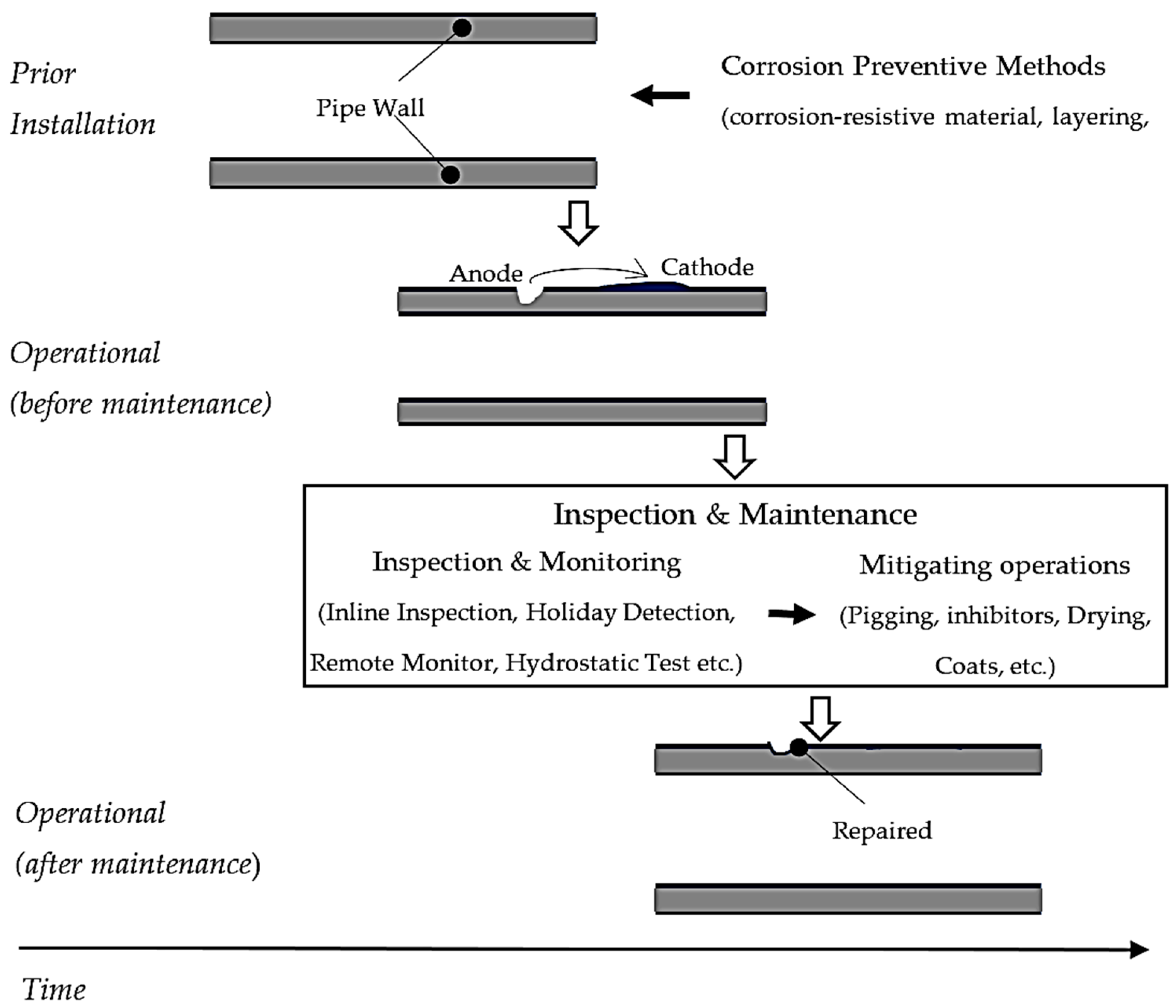
Corrosion is an electrochemical process where pipe wall materials are eroded from one location and deposited into another (Figure 1). There are different types of pipeline corrosion which include uniform or general, galvanic, crevice, pitting, and microbial [10]. Pipeline corrosion can be prevented by different methods, such as selecting corrosion-resistive material, layering external protective coats, and applying cathodic protection [11]. Various mitigation methods can be employed when corrosion occurs to minimize the impact and extend the service life of pipelines. These mitigation operations include pigging (maintenance operation using pipeline integrity gauge), adding corrosion inhibitor chemicals, drying, adding biocide, and applying coats and cathodic protection [12]. The selection of these methods depends on factors like cost, location of the corrosion defect, type of corrosion, and severity of the damage.

The corrosion maintenance can be implemented following a three-step procedure [13]. First, the latest state of the pipeline is examined through inspection or flow monitoring methods. This can be accomplished using ILI, holiday detection, above-ground monitoring, remote monitoring, hydrostatic testing, and below-ground inspection [12]. The growth of defects due to corrosion is estimated using stochastic or deterministic methods in the second step of the procedure. Deterministic methods include mathematical formulation such as single-value, linear, and nonlinear functions, whereas stochastic methods adopt MP, the time-dependent/independent generalized extreme value distribution, the Gamma process, and the Monte-Carlo simulation [14]. In the final step, maintenance operation parameters are optimized to exploit maintenance resources and the remaining service life of a pipeline.

3. Literature Review

Pipeline maintenance requires assessing the progression of defects followed by implementing optimal maintenance operations. The pipeline’s condition at the time of maintenance is crucial in determining the type as well as the cost of operation. This maintenance policy is commonly referred to as condition-based maintenance (CBM) in the literature. Abbasi et al. [15] defined three different condition-based maintenance approaches based on the methods used to determine the pipe states: model-based (adopt a mathematical model), knowledge-based (leverage available data using different artificial intelligence algorithms), and parameter-based (measure the pipe’s operational characteristics). The assessments can be performed on periodic or non-periodic time bases.

The implementation of CBM using Markov processes has been observed in several studies. The existing model formulations considered corrosion processes, the resulting failure, maintenance/inspection intervals, and optimal maintenance operations to mitigate the damage due to corrosion. For example, Valor, et al. [1] studied a pure birth process with Kolmogorov’s forward equation to generate the transition probability for a Markov process modeling of pitting corrosion. Yusof, et al. [2] demonstrated the effectiveness of a Markov chain model in predicting pitting corrosion growth. The study compared the result of the model to a fitted distribution function for the pipeline deterioration historical data. Ossai and Davies [3] presented a pure birth Markov model to predict pit corrosion depth using negative binomial distribution for transition probability formulated based on different factors (pit depths, temperatures, CO2 partial pressures, pH, and flow rates). Casanova-del-Angel, et al. [4] modeled the cumulative damage due to the propagation of internal corrosion (formulated with exponential functions) using the Markov chain to predict failure. It adopted Bernoulli trials and probability to make transition decisions. Tran, Setunge, and Shi [16] proposed a Markov model for determining the inspection interval of stormwater pipes. A Markov model was developed to emulate the pipe deterioration process, which was incorporated into a simulation model to run different maintenance planning scenarios. Jimenez-Roa, et al. [17] presented a Markov chain sewer pipe degradation model with single and multi-transition chains. Sequential Least-Squares Programming optimized the parameter for the Markov chain model by minimizing the root mean weighted square error. Zhao, et al. [18] integrated a machine-learning algorithm with the Markov chain and set pair theory to determine the reliability of anticorrosion coating. The model evaluated the change in the properties of the coating layer to establish its grade and effectiveness.

MDP and POMDP models have been recently adopted for maintenance-related optimization problems in the oil and gas industry. Heidarydashtarjandi, et al. [5] and Bediako, et al. [6] proposed MDP models to optimize maintenance actions. The degradation of pipelines based on physical attributes was determined using Monte Carlo simulation and non-stationary Gamma distribution models, respectively. The articles employed ILI and simulation data pipeline states assessment. Yinka-Banjo, et al. [19] discussed the application of unmanned vehicles as an inspection tool and implemented MDP as a maintenance optimization model. Compare, et al. [8] and Wari, et al. [7] demonstrated the implementation of the POMDP for two different optimization problems. Compare, et al. [8] optimized maintenance action along with some economic analysis for gas transmission networks. Wari, et al. [7] focused on the maintenance action considering partially observed states with ILI inspection errors. Most Markov-based maintenance optimization models assumed that the deterioration state of the pipeline could be accurately observed. In practice, accurate observation is challenging due to the dynamic nature of corrosion and the inherent error of inspection methods. Wari, et al. [7] addressed this problem by formulating a discrete state partially observable Markov decision process (DSPOMDP) model that considers observational errors and inaccuracies. This study extends the DSPOMDP approach by formulating the state as a continuous function to integrate the uncertainty without any discretization step. Better model fidelity can be achieved with this continuous state approach.

Exploring the POMDP model application is ongoing in several other industries and fields of study. Some of the most recently accomplished studies include Deep et al. [20], who integrated POMDP in maintenance planning optimization (with a case study for lead battery maintenance); Morato et al. [21], who combined dynamic Bayesian networks with POMDPs to formulate a framework for the optimization of inspection and maintenance planning; and Guo & Liang [22] who optimized inspection interval for maintenance operation using POMDP model with Baum–Welch algorithm for parameters estimation.

The choice of the solver is one of the most crucial aspects of adopting MDP and POMDP models. Value iteration or policy iteration methods can be considered for small-size (less than thousands of states) and discrete MDP and POMDP models. However, these methods cannot be effectively applied to large-size (more than a hundred thousand states) or continuous space models. For POMDP models, Kurniawati [23] presented a systematic review of sample-based solvers based on the attributes of modeling components. The review covered most of the popular solvers. For models with a large state space (some continuous state), the study recommended adopting algorithms such as point-based value iteration (PBVI—samples beliefs from a set of beliefs constructed from a reachable belief from a given initial belief), Perseus (sampling beliefs and backup operation performed independently), heuristic search value iteration (HSVI—employs an α-vector policy representation and point-based backup), successive approximations of the reachable space under optimal policies (SARSOP—a belief sample method using α-vector policy representation and point-based backup), and Monte Carlo value iteration (MCVI—a policy based algorithm where the total expected value is computed at a given point in a defined state and action). Monte Carlo tree search (MCTS—combination approach of random sampling and tree search in a balanced effort between exploitation and exploration [24]), and determinized sparse partially observable tree (DESPOT—for each iteration, the algorithm searches the sample space for the best policy for a belief state [25]) were proposed for continuous state (large state) POMDP models. Perseus and guided cluster sampling (an algorithm that optimizes on a subset of continuously updating sampling space) were suggested for continuous action POMDP models. Partially observable Monte Carlo planning (POMCP) and partially observable Monte Carlo planning with observation widening (POMCPOW—extensions of MCTS by adding Monte Carlo updating procedure for belief state to MCTS search in the present state [26]) have been proposed for POMDP models with a large number of observations. In addition, the review has presented several algorithms for long planning horizons and complex dynamic problem models. Even though the model elements encompassed in all algorithms are the same, the detailed formulation, solving procedures, effectiveness, and the final solution quality can differ. The proposed CSPOMDP model adopts the POMCP and DESPOT solvers to search for the best maintenance policies.

4. POMDP Model Formulations

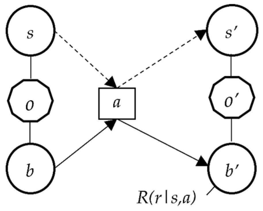
A POMDP model comprises the following elements (Figure 2):

• States (S)—defines a system’s condition (core state) in a dynamic environment. All possible states for the system are collected into a set (S). The two important states for analysis are the current state (s) and succeeding state (s′).
• Action (A)—is a collection of decisions (action—a) taken based on the state of the system (defined as a set—A).
• Transition probabilities (T(s′ |s, a)—is a matrix that defines the probability of landing on a specific succeeding state (s′) from a given current state (s) after taking action (a).
• Reward (R(s, a))—is a function that defines the cost (or reward) of taking a given action (a) on a system in a given current state (s).
• Observation (o) and observation probability (P(o|s, a)) have been added as elements in the model formulation. The observation is any description that can be obtained through a different mechanism and used to determine the actual state of the system. It is defined as a set (O). Observation probability is a matrix that defines the probability of observing o for a system in state s and after taking action a.
• Belief state (b(s)) is created to replace the states defined in the MDP model. The analysis of POMDP models uses these belief states, which define the degree (probability) of finding the system in a given MDP state (core state).

The belief states of a POMDP model can be formulated as a finite number of states (discrete state POMDP—DSPOMDP) or continuous states using different functions (CSPOMDP). Both formulation approaches can help attain deeper core state analysis. The continuous function formulation of the belief state has been extended to the observation probability and action, which is collectively called continuous space POMDP. For a large number of (continuous) states, observations, and actions, continuous space modeling methods can be more effective even though finding optimal results could be very difficult due to model complexity (refer [26,27] for detailed discussion).

In DSPOMDP, the system transitions into a succeeding state based on the transitional probability, action, and current state. The system’s succeeding belief state is obtained through a belief-updating computation using Bayes’ rules. For a CSPOMDP, the update is computed by integrating the expected belief states rather than summing, which is the case for discrete formulation [27,28]. P(o|s′, a) was normalized by dividing it with the probability of observing o under known action a and current belief state b(s) (P(o|b, a)). This normalizing factor was computed by adding the expected probability of the observation o for all succeeding states based on the current belief state. The new belief state (b′ (s′)) is computed by multiplying this normalized value by the expected belief of transitioning from the current state to the succeeding state, an integral function (Equation (1)). An MDP model with infinite dimensional core states (to constitute the belief states) can represent a CSPOMDP [27].

$$b^{\prime }\left(s\prime \right)=\frac{P\left(o|s^{\prime },a\right)}{P\left(o|b,a\right)}{\int }_{s\in S}P\left(s^{\prime }|s,a\right)b\left(s\right)$$

(1)

where

$$P\left(o|b,a\right)={\sum }_{s^{\prime }\in S}P\left(o|s^{\prime },a\right){\sum }_{s\in S}P\left(s^{\prime }|s,a\right)b\left(s\right)$$

The total reward (V(b)) is computed at each step of POMDP. For a given action, it is the sum of the integral of the expected marginal reward from a belief state and the discounted expected rewards of all preceding belief states. The discounting factor (γ) controls the impact of older belief states values on the latest value. The optimal value (V*(b)) is determined by comparing the values obtained from all actions (Equation (2)).

$$V*\left(b\right)=\underset{a}{\max }(({\int }_{s^{\prime }\in S}r\left(s^{\prime },a\right)b\left(s^{\prime }\right))+\gamma {\sum }_{o\in O}P\left(o|b,a\right)V*\left(b\right))$$

(2)

where

$$r\left(s^{\prime },a\right)={\sum }_{s\in S}{\sum }_{o\in O}r\left(s^{\prime },a,s,o\right)P\left(s|s^{\prime },a\right)P\left(o\right|s,a)$$

As the size of the core states increases, solving the POMDP problems can become computationally difficult. In these cases, the solution approach developed for discrete POMDP will render useless due to the explosion of belief states. Overall, continuous space POMDP (large-size discrete space POMDP) poses computational challenges that emanate from the curse of dimensionality and history [28]. The curse of dimensionality describes the challenges that arise from the POMDP model becoming computationally expensive as the size of the model increases, whereas the curse of history originates from the difficulty of tracking actions and observations as these model components grow exponentially.

Two solvers were selected to optimize the POMDP formulations: POMCP and DESPOT. The selection criteria mainly focused on the algorithm’s capability to optimize continuous-state POMDP problems. POMCP combined the Monte Carlo simulation and tree search methods. It is an extension of the Monte-Carlo-based tree search (MCTS) algorithm that assesses the value of the belief state in each branch of a search tree to identify the most promising chain of states in the search space [24]. POMCP incorporates particle filters (unweighted) to facilitate the search [26]. A generative function was used to select the succeeding state, available action, and observation formulate to the search problem in each iteration, which loosens the requirement for explicit definition of the transition and observation probability. Further extension of POMCP was proposed by Sunberg and Kochenderfer [26], named Monte Carlo planning with observation widening (POMCPOW), where particle filters were included in the observation function so that a single particle cannot dominate the solution search. Sunberg and Kochenderfer [26] also proposed particle filter trees with double progressive widening (PFT-DPW) to improve the limitations of POMCP. Determinized sparse partially observable tree (DESPOT) is a sampled scenario based on an online POMDP solver (adopting an anytime heuristic algorithm) where the evaluation of values for each action guides the decision-making [25]. An anytime heuristic algorithm is a search algorithm designed to reach a solution sequentially with an allocated run time [29].

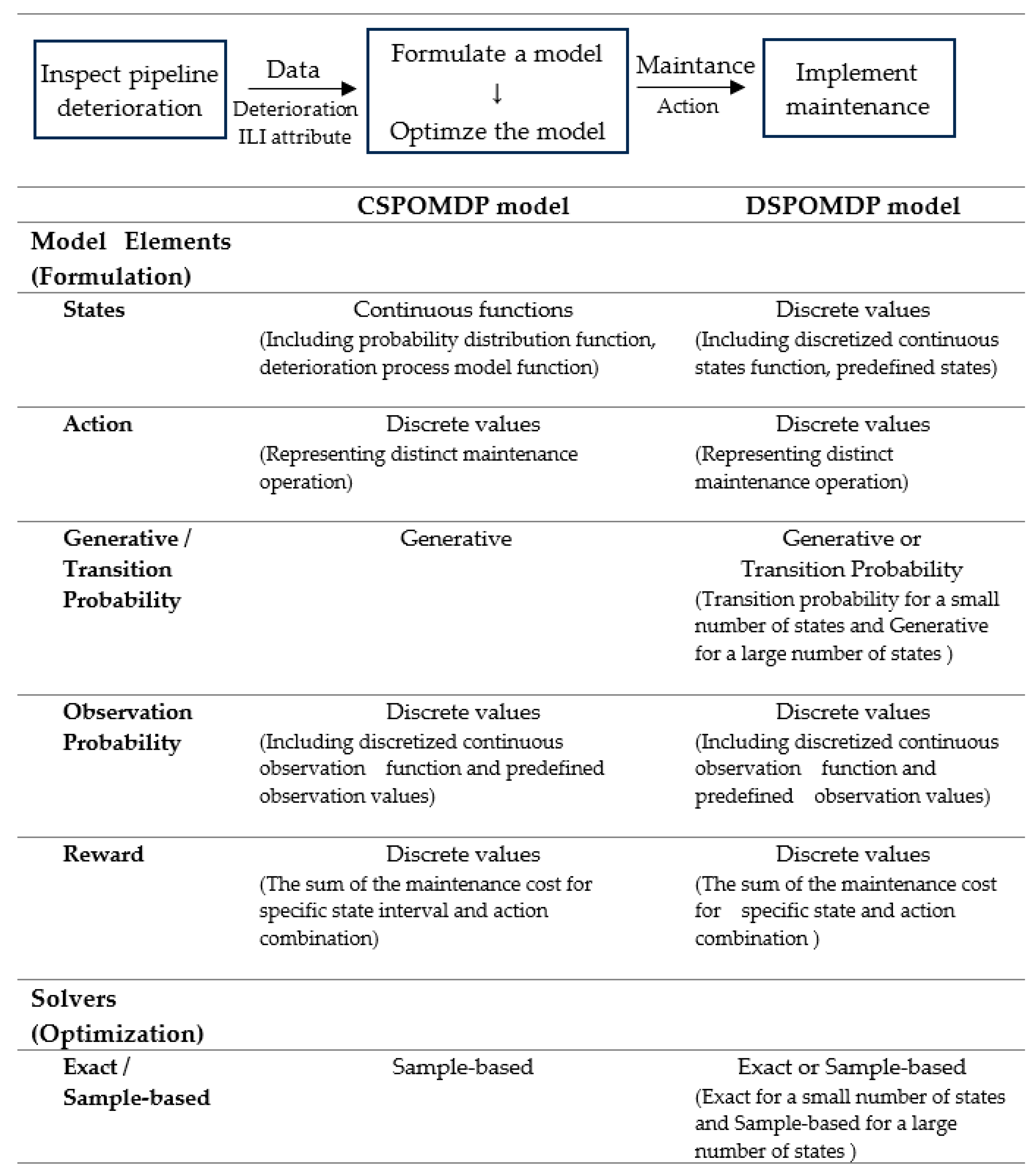
Implementing the POMDP to corrosion maintenance optimization requires adopting this general formulation model. An appropriate solver will then be implemented to attain the recommended maintenance action. A summary of the two-model formulation (i.e., CSPOMDP and DSPOMDP) is given in Figure 3, while the following sub-sections discuss the details of the formulation.

4.1. CSPOMDP Model

The proposed CSPOMDP model consists of most of the elements of the standard formulation. In addition to the current state, actions, observation function, and reward, a generative function was included to select the succeeding state randomly. The details of these model components are discussed in this section.

4.1.1. State

The pipeline system corrodes over time in a continuous process. The continuous state formulation tries to emulate this degradation process. Pipeline degradation due to corrosion comprises two distinct steps: formation corrosion and growth or propagation of the corrosion. The formation process can be a Poisson distribution process or negative binomial distribution [30,31]. The Markov process, Gamma distribution, and Monte Carlo simulation can describe the continuous progression of corrosion. The two steps can also be combined to formulate the complete corrosion degradation process. For this approach, the Markov process was frequently adopted in the literature [5,32]. This later approach has been extended with an inspection process to determine the latest degradation state of the pipelines.

The current degradation state of the pipeline was attained from the inspection report. However, the decisions and rewards depend on the succeeding state, which has to be estimated by the POMDP model. The actual degradation of the pipeline was defined as a percentage of the wall thickness. This is measured by an inspection method or a model that predicts the degradation. Different upper and lower limits for the degradation state can be established to recommend the most effective mitigation action. A maximum degradation state should have to be set so that the pipeline will be replaced when reaching this state.

4.1.2. Action

Pipeline maintenance operations focus on mitigating the damage due to corrosion degradation. Some of the mitigating methods have been presented in Section 2. Adding inhibitors and applying the coating could reduce the degradation process efficiently at an earlier stage of the pipeline service life. As pipelines age, the damage becomes severe, requiring more invasive methods such as pigging. Pigging utilizes pipeline integrity gauge (pig) tools that flow with the product and repair pipeline defects. These pigs are not only used for repairs but also for cleaning and inspecting pipelines.

The action element in the model can be based on the degradation state of the pipeline in order to attain the maximum result from the maintenance operation. This is achieved by restricting the implementation of each mitigation method discussed above to an interval degradation state. Overlap of application regions may arise in this formulation, where the model selects the best option based on the reward obtained. The action set can also include no action alternative (do-nothing) to perform only inspection. Replace actions can be recommended when the degradation of the pipeline goes beyond the allowed limit.

4.1.3. Observation

The true degradation state of the pipelines is hard to determine due to several factors. However, various methods can be implemented to estimate the current states which were used to formulate the model. ILI using different tools has commonly been used in the industry. The tools included magnetic flux leakage, ultrasonic, electromagnetic, and acoustic technology, and eddy current testing [14]. Mathematical models can also be used to estimate the degradation based on the progression behavior of corrosion or the operational parameters of the pipeline.

The error in the estimation can be used to formulate the observation function. For an ILI, equipment errors emanate from four sources: detection, sizing or measuring, false call, and reporting threshold [33]. Detection errors arise from the inability to detect the due corrosion size. Smaller-sized defects have a low probability of detection. Sizing is a random error due to the intrinsic nature of the equipment. The normal distribution function is used to estimate this error [30]. Equipment creates a false call error when it reports a non-existing defect in the pipeline. This error occurs mostly to large-sized defects using poor-quality inspection equipment. Threshold reporting refers to the detection range of equipment. Any defect beyond this range will not be detected, creating a detection error. Zhang and Zhou [30] and Dann and Maes [33] have proposed several mathematic formulations for these errors. In addition to the equipment errors, the observation formulation can incorporate inspection personnel errors (reading errors) and errors emanating from the pipeline operating environment. Historical or empirical data or mathematical models can be used to compute the errors and formulate the observation function.

Continuous observation functions would have to be discretized for a discrete model before integrating them into a discrete space POMDP. The observation range can be divided into equal intervals to create discrete values. Alternatively, an advanced discretization mathematical method can be applied to construct the values. When the observation matrix is generated, the pipeline state can take multiple observation values (expressed as a probability function) or a specific value. It is important to note that this discretization step is skipped for a continuous observation POMDP model to incorporate the function directly.

4.1.4. Reward

Rewards are formulated as the sum of all maintenance-related costs for a given action taken under a specific pipeline state. Corrosion-mitigating activities discussed above incur a different amount of cost to implement. These costs include production downtime, spare parts acquisition, repair operation, and any flow compensation costs that are computed using organizational data. Heidarydashtarjandi et al. [5] considered the cost associated with the risk of failure in estimating the reward. It is computed as the product of the failure risk and the respective cost of the failure. Expert options and historical data can serve as a source of input for this computation. When multiple inspections are considered in the POMDP model, the inspection cost can be added to the cost function.

The total cost (TC_S,A) was defined as the total reward obtained for a given state and action (Equation (3)). It was computed as the sum of the maintenance operation cost (MC_S,A—for a given state and action), the failure cost (FC_S—for a given state), and the inspection cost. Failure costs aggregate the cost of different failures (leaks and raptures) based on their respective probability.

$${TC}_{S,A}={MC}_{S,A}+{FC}_S+I$$

(3)

where ${TC}_{S,A}$—the total cost (reward);

${MC}_{S,A}$—the cost of maintenance;

${FC}_S$—the failure cost = ${\sum }_{f\in Failures}{Prob}_f\times {Cost}_f$;

I—the inspection cost.

4.2. DSPOMDP Model

The DSPOMDP model is mainly included to provide background information on the formulation. Two formulations were used for the model: a discretized version of CSPOMDP and a modified DSPOMDP from Wari et al. [7].

• State—For the first model, a discrete state discrete model was created by converting the continuous random distribution given above. The second model adopted the formulation from Wari et al. [7] with some modifications.
• Action—The same formulation as CSPOMDP.
• Transition probability—a generative function similar to CSPOMDP was used for the first formulation, whereas a transition probability was inherited from the article with some modification for the second.
• Observation—The CS model was modified for the first model, while the published formulation was applied for the second model.
• Reward—Similar formulation to the CS model was adopted, except for the modification to accommodate the discrete state formulation of DSPOMDP.

5. Numerical Examples

The proposed model was tested using numerical examples. The data for these examples were collected from the literature [5,7]. For example, Heidarydashtarjandi et al. [5] based their model on a pipeline with API 5L GX52 material type, 610 mm outer diameter, and Normal (447 mm, 19 mm) wall thickness. The study focused on the maintenance of pitting corrosion with either ILI or pipeline operating conditions data. The DSPOMDP model adopted some of the numerical data from this study. Khan, et al. [34] reported multiple Weibull and Gumbel models for pipeline deterioration based on ILI (Magnetic Flux Leakage) for pipelines with 7.1 mm and 7.9 mm wall thickness (mild steel material) that extends over 250 Km. The Weibull deterioration function was modified to formulate the CSPOMDP model states.

However, some additional data have been generated to complete the model formulation and test runs. The CSPOMDP parameters were constructed in a manner that was described in Section 3. Parameter descriptions for two DSPOMDP models were included for each model element. Experimental runs compared the results of the CS against the DS models to show the performance of the proposed formulation.

5.1. Model Parameter Definition

Numerical values have been assigned to the POMDP model elements to implement the optimization process. These elements were defined for a continuous space. However, to provide a reference for comparison, a discrete problem formulation was also considered in this section.

• States (S): A continuous function was used to describe the level of pipeline deterioration as the percentage of the pipeline wall thickness (s = [0.0, 0.95]). A new pipeline would have a deterioration level close to 0% of the wall thickness, whereas a failed pipeline would have a value close to 95%. The initial state of the new pipeline was randomly determined using a normal distribution with a mean of 0.05 and a standard deviation of 0.003. The probability of landing at a specific state (s′) depended on the initial state and action taken (

  Table 1. Succeeding state (s′) probability for CSPOMDP.

  Current State (s) Value	Action
  	Do-Nothing	Inhibitor	Pigging	Replace
  0.00–0.15	0.15 + 0.85 × (rand(Weibull(1.19, 0.69)))	0.13 + 0.7 × rand(Weibull(1.19, 0.35))	0.15 + 0.85 × (rand(Weibull(1.19, 0.69)))	rand(Normal(0.05, 0.003))
  0.15–0.35	0.35 + 0.65 × (rand(Weibull(1.19, 0.69)))	0.13 + 0.87 × (rand(Weibull(1.19, 0.35)))	0.35 + 0.65 × (rand(Weibull(1.19, 0.69)))	rand(Normal(0.05, 0.003))
  0.35–0.6	0.6 + 0.4 × (rand(Weibull(1.19, 0.69)))	0.6 + 0.4 × (rand(Weibull(1.19, 0.69)))	0.45 + 0.55 × (rand(Weibull(1.19, 0.35)))	rand(Normal(0.05, 0.003))
  0.6–0.85	0.85 + 0.13 × rand(Weibull(1.19, 0.35))	0.85 + 0.13 × rand(Weibull(1.19, 0.35))	0.5 + 0.5 × (rand(Weibull(1.19, 0.35)))	rand(Normal(0.05, 0.003))
  >0.85	rand(Normal(0.95, 0))	rand(Normal(0.95, 0))	rand(Normal(0.95, 0))	rand(Normal(0.05, 0.003))

  ). The specific value of the state was formulated as a function of Weibull distribution with a fixed lower bound to ensure the gradual deterioration of the pipeline [34]. For example, when the pipeline is in the deterioration range between 0.00 and 0.15 (0–15%) and a Do-nothing action is taken, the succeeding state is estimated by a random function (0.15 + 0.85 × (rand (Weibull (1.19, 0.69)))). Table 1 presents the random function that defines the probability distribution of the succeeding state for a CSPOMDP.

The discrete version of the succeeding state probability distribution (for five core states) is given in

Table 2. Succeeding state (s′) probability for DSPOMDP.

Current State (s) Value	Action
	Do-Nothing	Inhibitor	Pigging	Replace
1	1 + min (round (10 × rand (Weibull (1.19, 0.69))), 4)	1 + min (round (10 × rand (Weibull (1.19, 0.35))), 4)	1 + min (round (10 × rand (Weibull (1.19, 0.69))), 4)	rand(SparseCat([1], [1.0]))
2	2 + min (round (10 × rand (Weibull (1.19, 0.69))), 3)	1 + min (round (10 × rand (Weibull (1.19, 0.35))), 4)	2+ min (round (10 × rand (Weibull (1.19, 0.69))), 3)	rand(SparseCat([1], [1.0]))
3	3 + min (round (10 × rand (Weibull (1.19, 0.69))), 2)	3 + min (round (10 × rand (Weibull (1.19, 0.69))), 2)	2 + min (round (10 × rand(Weibull(1.19, 0.35))), 3)	rand(SparseCat([1], [1.0]))
4	4 + min (round (10 × rand (Weibull (1.19, 0.69))), 1)	4 + min (round (10 × rand (Weibull (1.19, 0.69))), 1)	3 + min (round (10 × rand(Weibull(1.19, 0.35))), 2)	rand(SparseCat([1], [1.0]))
5	rand(SparseCat ([5], [1.0]))	rand(SparseCat([5], [1.0]))	rand(SparseCat([5], [1.0]))	rand(SparseCat([1], [1.0]))

.

• Actions (A): Four maintenance actions have been considered in the model, i.e., Do-nothing, Inhibitor, Pigging, and Replace. The implementation of these actions was as per the discussion of these maintenance actions in Section 3. The same application principles have been adopted for both discrete and continuous models.
• Observation (O): The observation represented the range of readings that an ILI reported as the succeeding state after performing an action. It is a discrete value ranging from 0% to 95%. A function was used to determine the observed value for a given succeeding state (s′). A maximum of ±15% variation in reading the state was assumed for the continuous observation (taken from [7]).

$$O\left(s^{\prime }\right)=\left\{\begin{array}{cc}\hspace{1em}\hspace{1em}0\hfill & if s^{\prime }=0.0\hfill \\ {round(s}^{\prime }\ast 100)+random\left(-d:d\right)& if 0<s^{\prime }<0.95\hfill \\ \hspace{1em}\hspace{1em}95\hfill & if s^{\prime }=0.95\hfill \end{array}\right.$$

(4)

where s′ = succeeding deterioration level and d = variation value.

For the discrete model observation, Equation (4) was converted into a function that creates variation to only five states reading. Equation (5) gives this formulation.

$$O\left(s^{\prime }\right)=\left\{\begin{array}{cc}\hspace{1em}\hspace{1em}1\hfill & if s^{\prime }+round\left(\frac{random\left(-d:d\right)}{10}\right)\le 1\hfill \\ s^{\prime }+round\left(\frac{random\left(-d:d\right)}{10}\right)& if 1<s^{\prime }+round\left(\frac{random\left(-d:d\right)}{10}\right)<5\hfill \\ \hspace{1em}\hspace{1em}5\hfill & if s^{\prime }+round\left(\frac{random\left(-d:d\right)}{10}\right)\ge 5\hfill \end{array}\right.$$

(5)

where s′ = succeeding deterioration level and d = variation value.

The probability of reading multiple states was formulated as a function for a single succeeding state for the second DS model. The original approach (defined eight-state model) has been modified to a five-state model to fit the current formulation (

Table 3. Discrete observation probability of succeeding state (s′).

State (S)	Observation (O)
	1	2	3	4	5
1	1	0	0	0	0
2	0	0.9	0.1	0	0
3	0	0.1	0.6	0.5	0
4	0	0	0.3	0.5	0
5	0	0	0	0	1

).

• Reward (R): The reward function, defined as the cost of performing maintenance, computed the total of two types of costs based on the current state and action. These costs comprised the maintenance and inspection (fixed amount) costs. The maintenance cost is the operational cost, including labor, spare parts, equipment, and other related expenses. Discrete values described these rewards values. Thus, the continuous states have been grouped into ranges that, in most cases, can represent real-world situations.

  Table 4. Reward (cost) function.

  Current State (s) Value		Action
  Discrete POMDP	Continuous POMDP	Do-Nothing	Inhibitor	Pigging	Replace
  1	0.00–0.15	−200	−2000	−4000	−5000
  2	0.15–0.35	−500	−350	−3500	−5000
  3	0.35–0.6	−800	−300	−400	−5000
  4	0.6–0.85	−2000	−5000	−450	−2250
  5	>0.85	−5000	−5000	−3000	−250

  presents the reward/cost for both modeling cases.

• Generating function/Transition probability: To address the modeling challenge arising from the infinite belief state, a generative function was created to estimate the succeeding state, which was used to compute the observation and reward value for given action. This generation was iteratively performed to search for the best action for different states in the solution space. The procedure for this function is:
  • Obtain the current state and action taken;
  • Randomly select a succeeding state (Table 1 or Table 2);
  • Compute the observation of the succeeding state (Equation (3));
  • Estimate the reward (Table 4);
  • Report the succeeding state, observation, and reward.

Table 5. Discrete state transition probability.

Do-Nothing						Inhibitor
State (s′)	State (s)					State (s)
	1	2	3	4	5	1	2	3	4	5
1	0.01	0	0	0	0	0.15	0	0	0	0
2	0.598	0.524	0	0	0	0.85	0.75	0	0	0
3	0.299	0.342	0.536	0	0	0	0.25	0.536	0	0
4	0.016	0.019	0.032	0	0	0	0	0.032	0	0
5	0.077	0.115	0.432	1	1	0	0	0.432	1	1
Pegging						Replace
	State (s)					State (s)
	1	2	3	4	5	1	2	3	4	5
1	0.01	0	0	0	0	1	1	1	1	1
2	0.598	0.524	0	0	0	0	0	0	0	0
3	0.299	0.342	0.7	0	0	0	0	0	0	0
4	0.016	0.019	0.3	0.75	0	0	0	0	0	0
5	0.077	0.115	0	0.25	1	0	0	0	0	0

presents the transition matrix Wari et al. [7] proposed, which was applied to the second DSPOMDP model.

5.2. Experimental Runs Results

BasicPOMCP and ARDESPOT, Julia language-based POMDP solver package solvers (part of Julia-POMDPs packages), were used to solve the continuous POMDP model [9]. BasicPOMCP adopted the basic POMCP formulation proposed by Silver [24], whereas ARDESPOT followed the pseudo-code presented by Ye et al. [25]. JuPython (with Julia 1.7.2) formulated and ran both models. An MSI GT72S 6QE Dominator laptop with Intel Core i7-6820 and 48 GB RAM was used to compute the models.

Three experimental runs of the models were conducted to assess the performance of the proposed approach. The first run described the solution search processes that each solver undertook. This was conducted using smaller-size models. The second run aimed to compare the modeling method’s performance, where a medium-size problem model was considered. Finally, different maintenance policies were evaluated to test the maintenance decision-making process and maintenance policies.

5.2.1. Experiment 1

A five-step tree search was performed using BasicPOMCP and ARDESPOT solvers for the continuous model described above (

Table 6. Example of CSPOMDP model run result using POMCP.

s	a	s′	o (%)	r
0.051	Do-nothing	0.649	66	−200
0.649	Replace	0.051	0	−2250
0.051	Do-nothing	0.488	57	−200
0.488	Do-nothing	0.717	80	−800
0.717	Replace	0.052	15	−2250
Discounted (0.9) total reward/cost =				−4446.43

and

Table 7. Example of CSPOMDP model run result using ARDESPOT.

s	a	s′	o (%)	r
0.051	Do-nothing	0.180	19	−200
0.180	Inhibitor	0.182	11	−350
0.182	Do-nothing	0.420	50	−500
0.420	Inhibitor	0.613	69	−300
0.613	Pigging	0.518	62	−450
Discounted (0.9) total reward/cost =				−1433.95

). With the same initial state of the pipeline, the two solvers took maintenance action based on the succeeding states that each randomly landed on. The observation considered the reading variation of the ILI method and gave the reading obtained as the percent deterioration. The current state and action taken determined the reward (cost) in each step of maintenance service. The discounted aggregate of these costs defined the total reward of the campaign.

The DSPOMDP model run results are given in

Table 8. Example of DSPOMDP model run results.

First DSPOMDP Model					Second DSPOMDP Model
POMCP					POMCP
s	a	s′	o (s′)	r	s	a	s′	o (s′)	r
1	Inhibitor	4	4	−2000	2	Do-nothing	2	2	−500
4	Replace	1	1	−2250	2	Inhibitor	2	2	−350
1	Do-nothing	5	5	−200	2	Do-nothing	2	3	−500
5	Replace	1	2	−250	2	Pigging	5	5	−3500
1	Do-nothing	1	2	−200	5	Replace	1	1	−250
Discounted (0.9) total cost =				−4500.47	Discounted (0.9) total cost =				−4488.19
ARDESPOT					ARDESPOT
s	a	s′	o (s′)	r	s	a	s′	o (s′)	r
1	Do-nothing	3	3	−200	2	Do-nothing	2	2	−500
3	Inhibitor	4	3	−300	2	Inhibitor	2	2	−350
4	Do-nothing	4	5	−2000	2	Inhibitor	2	3	−350
4	Replace	1	2	−2250	2	Inhibitor	3	3	−350
1	Do-nothing	3	4	−200	3	Inhibitor	5	5	−300
Discounted (0.9) total cost =				−3861.47	Discounted (0.9) total cost =				−1692.81

. The initial state of the pipelines was assumed to be the same for both models. Since the succeeding state differs, various maintenance actions were undertaken, contrasting total costs. Unlike the CS model results, the observation results reported the state that the ILI method obtained. This reading sometimes varied from the true state (s′) due to the above-mentioned errors.

5.2.2. Experiment 2

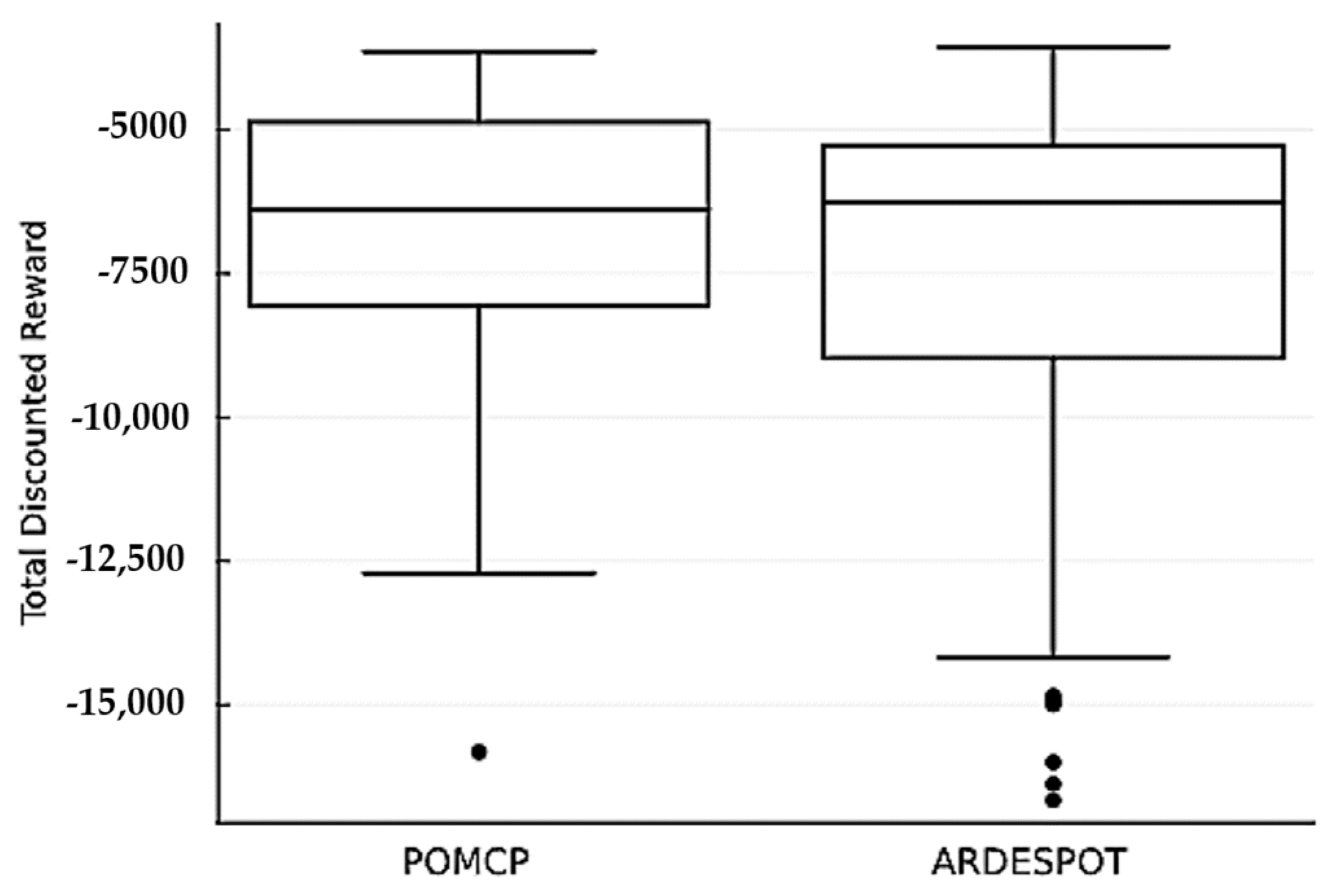
Although the initial state of the pipeline was set to be the same, the total cost after multiple maintenance services varied due to the stochastic nature of the succeeding state selection and actions taken based on uncertain observations. A medium size maintenance service campaign (32 steps) replicated 100 times was run for this second test to assess this feature of the model. The two solvers were also implemented for the CS and DS problem models.

Figure 4 shows the distribution of the total cost (reward) of the CSPOMDP model using the POMCP & ARDESPOT solver. Since the two plots overlap, the two model run results did not differ significantly (−7717 and −4567 for POMCP and −11,591 and −5809 for ARDESPOT 25 and 75 percentile values). Overall, the POMCP results looked better with cheaper cost distribution. It can be observed that there were some outliers in both solvers’ run results.

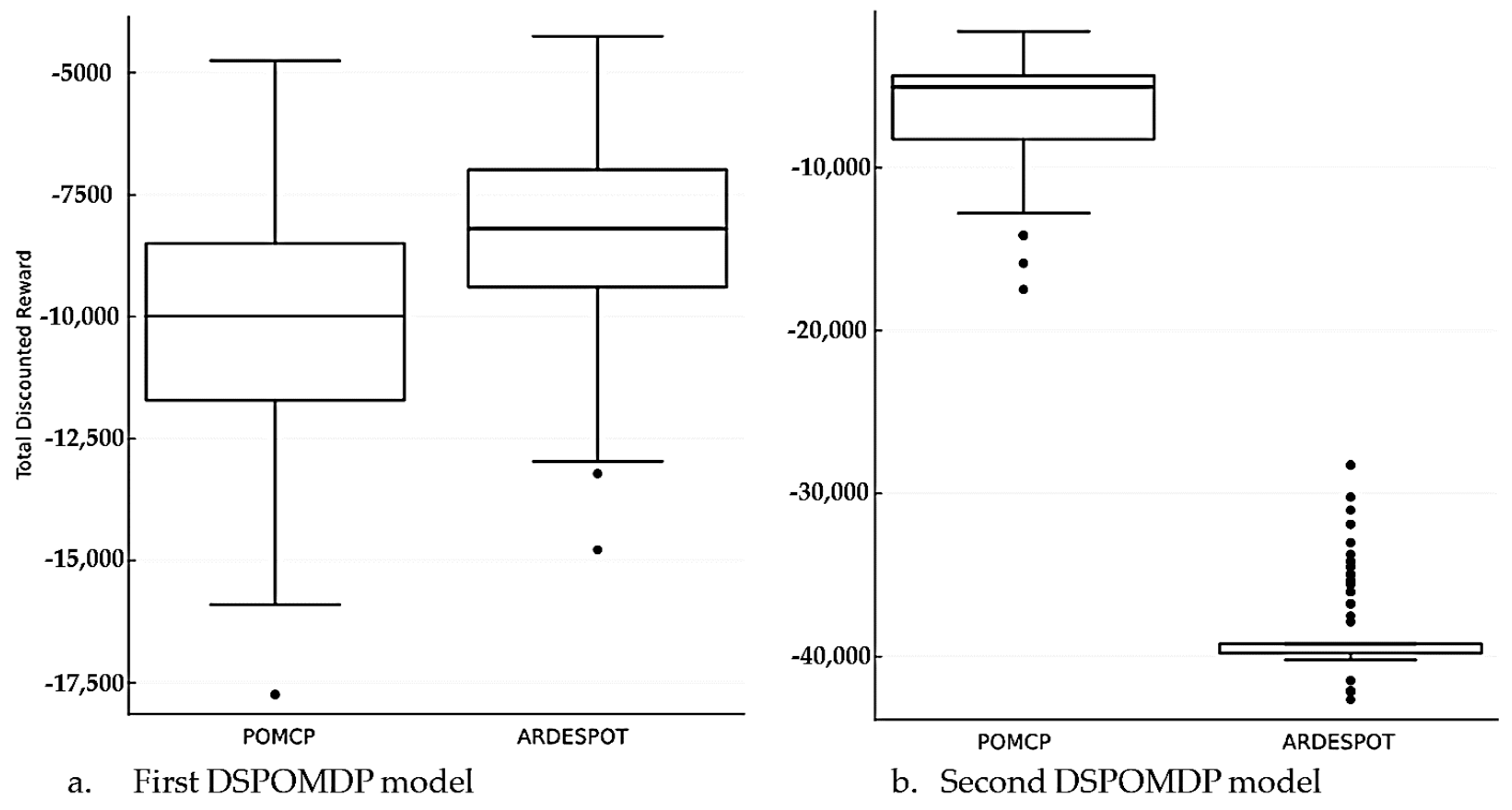
For the first DSPOMDP model, the POMCP and ARDESPOT attained similar 25 and 75-percentile values, i.e., −13,819 and −9725 and −12,370 and −8607 (Figure 5a). The ARDESPOT results overlapped with the result obtained for CS, unlike the result for POMCP. The 25 and 75 percentile values for the second DSPOMDP model were −8315 and −4488 and −39,774 and −37,096 for POMCP and ARDESPOT solvers, respectively (Figure 5b). This result showed a major difference between the two solvers. However, only the ARDESPOT significantly varied when compared to the CS model.

5.2.3. Experiment 3

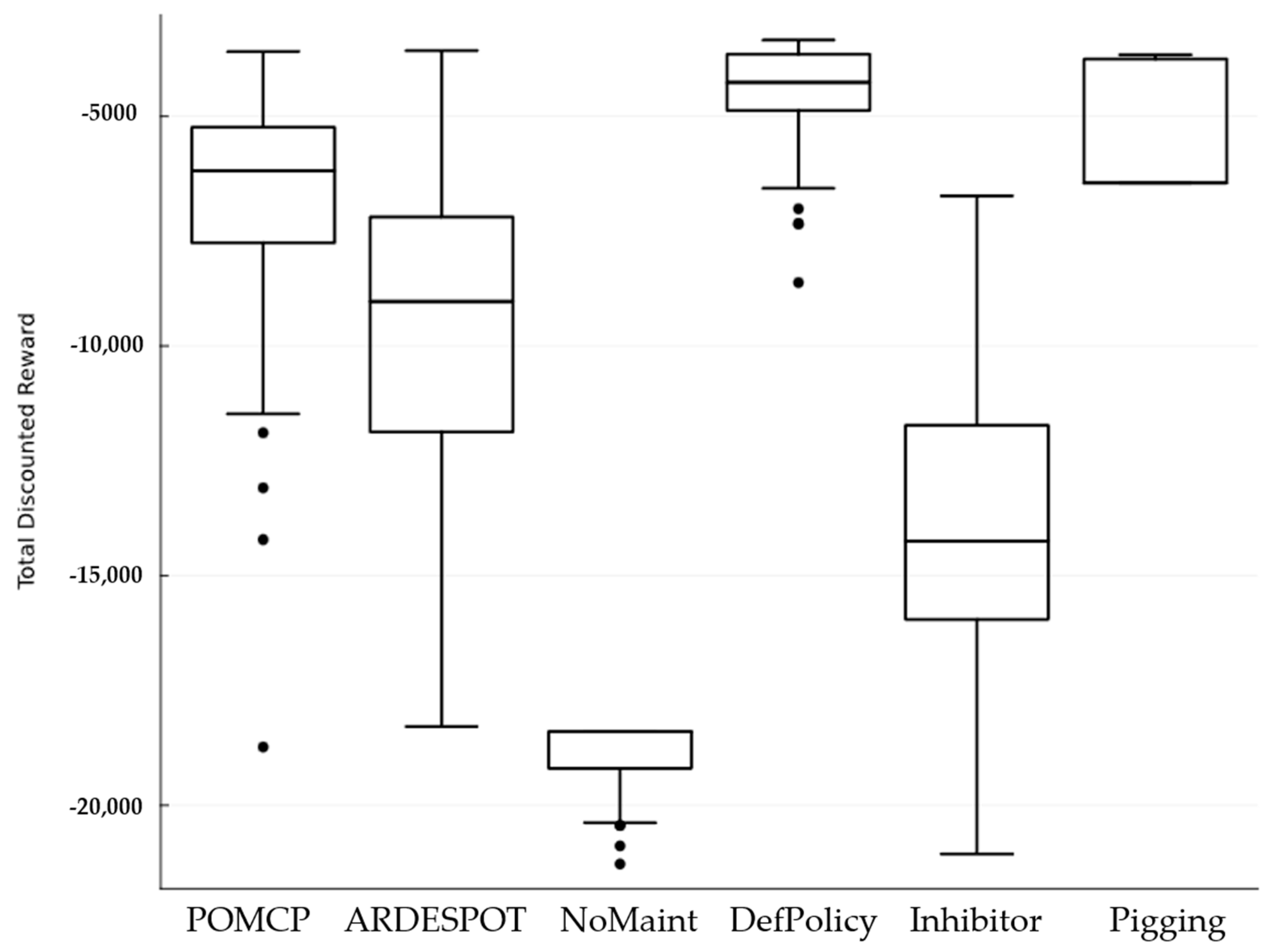
The last experiment compared the different policies adopted to solve the problem. The no maintenance policy (NoMaint) implemented the do-nothing action in each pipeline state except for the last state, where the pipeline would have to be replaced. The predefined policy was implemented by determining the maintenance action for a given state. This policy was labeled as DefPolicy. The effectiveness of implementing only inhibitors throughout the life of a pipeline was tested by setting the action to be inhibit for given states and do-nothing for all remaining others. Similarly, the pigging maintenance action was assessed by setting the action to pigging for some states and do-nothing for others.

For the CSPOMDP, the different policies have been implemented on a medium-size model similar to the one described in experiment 2 (Section 5.2.2). Figure 6 shows the resulting distribution for each policy’s discounted total cost. The box plot for each policy can be compared to assess the performance of each policy and determine the best alternative for implementation. The cost of each policy can also be estimated from these plots. Accordingly, the DefPolicy was the best policy, followed by Pigging, POMCP, ARDESPOT, and Inhibitor, while NoMaint was the worst of the alternatives.

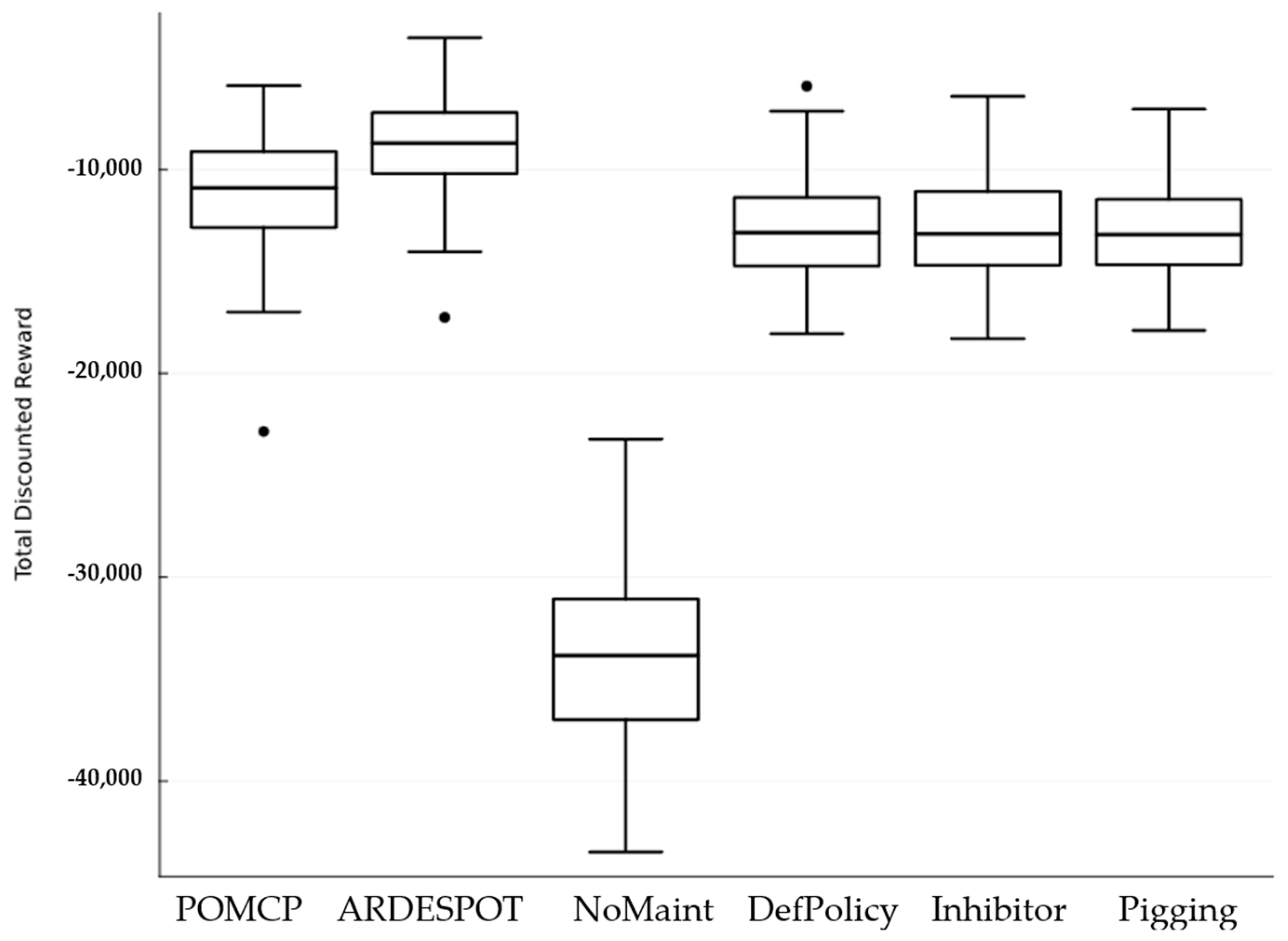
The DS model run was also performed for the policies described above. Figure 7 shows that ARDESPOT and POMCP were the better policies, and no significant differences could be made among DefPolicy, Pigging, and Inhibitor policies. However, NoMaint was observed to be the worst of all. Overall, the total cost was higher for this set of policy runs.

5.3. Discussion

CSPOMDP model formulated the corrosion level of the pipeline as a continuous process. The state definitions adopted continuous distributions, such as Weibull and Normal, to fit the corrosion process and forecast the corrosion level. An empirical function can also be substituted for these probability distributions using real-world data. To implement the DS modeling, these state definitions have to be converted to a discrete value, or the deterioration span needs to be divided into equally ranged levels. These discretization processes may cause a loss of pertinent modeling information about the state of the pipelines. Other elements of the modeling process are adjusted accordingly to accommodate these modeling changes. For example, most action, observation, and reward functions were defined to give a discrete reading since this is the standard practice on the ground. In the case of predefined policy implementation, a range of current states can be used to define preferred actions, primarily for CS models.

The CS POMDP model was tested at different levels of complexity with multiple policy settings. The CSPOMDP results were similar using either solver, even though the state transitions differed. Experiment 1 demonstrated that even though the initial state of the pipelines was the same, the final total reward obtained after multiple steps transition can vary. The stochastic process of the transitional states as well as the ILI reading of the state, contributed to these variations. Through replication of the model run, the uncertainty of the state transition, hence the total reward, can be improved to make better maintenance decisions. Experiment 2 showed this replication process results for both the CS and DS models. In general, increasing the number of replications reduced the uncertainty of total reward at the cost of run time. The impact model formulation variation between the CS and first DS models was minimal, as can be seen in Figure 4 and Figure 5a. Converting the CS model to DS can give improved results when compared to formulating the problem as DS model directly. However, the second DS model differs, especially when using the ARDESPOT solver. However, the solver selection does not clearly provide a distinction with regard to the total reward obtained. Therefore, the exact total reward assessment would have to be performed based on the best result from the two solvers. Finally, the results of experiment 3 showed the variation among different policies, which would aid decision-making. The CS POMDP provided better policy filtering, enhancing the chance of making better maintenance decisions. This advantage can be attributed to the more detailed state formulation in the CS POMDP. Since the solver attains random cost values in each run, considering results from multiple replications using multiple solvers would be advantageous.

Most model runs were completed within a short run (less than 5 s) using the above-described computing facility. The only exceptions were the model run for POMCP solver policy in experiment 3, which took 25–30 s, and ARDESPOT, which took 50–55 min. The time significantly increased for runs with more than 100 replications, requiring better computing facilities and longer execution times.

6. Conclusions and Future Work

Pipelines constitute a significant portion of assets in the oil and gas industries. They have a substantial impact on product flow throughout the supply chain. Ensuring pipelines’ safe operation is paramount in the industry, as evidenced by past catastrophic accidents. Effective maintenance functions can guarantee the continuous and reliable operation of pipelines. This study aims to contribute toward this goal.

Corrosion maintenance is performed by first inspecting the state of the pipeline using ILI methods. Based on the inspection output, the maintenance operation is optimized to minimize costs and prolong the service life. Since corrosion is a continuous process, it requires a continuous function to model better the defects it causes in pipelines. Furthermore, most ILI methods come with inherent reading errors, and addressing these errors inside the optimization model is very important to assess the effectiveness of ILI methods. Particularly, investigating the systemic error of the inspection method is essential to understand its overall impact on maintenance decision-making. The POMDP model proposed in this paper addressed a continuous state formulation while accounting for the observational variation due to inspection error.

The state of the proposed CSPOMDP model defined the deterioration level as a fraction of wall thickness. An upper bound for deterioration has been set to avoid the pipeline’s failure while in service. Corrosion mitigation methods such as adding inhibitors and pigging were formulated as actions. No maintenance action and total replacement have also been added to the action set to provide more decision options. The observation function has been fitted to the behavior of the ILI method, including the systemic error that the methods embody. Since most methods report the pipeline state as discrete values, the observations were formulated accordingly. The reward, defined as the cumulative cost related to a maintenance operation, was comprised of service and inspection costs. Hence, the objective of the optimization problem was to identify the least costly maintenance policy for the pipeline’s partially observed initial state.

POMCP and DESPOT, sample-based algorithms, were used to formulate a numerical test model to assess the CSPOMDP model’s performance. Compared to the discrete state model formulation, the continuous state showed slight variation in solution search proficiency and run-time. It showed better policy analysis due to the more elaborate definition of the states. However, optimal results cannot be obtained even in small-size problems. Experimental runs showed that the POMDP model could be adopted to compare maintenance policies defined by practitioners or obtained from solvers. This could help identify the best options, including those that may have been overlooked in the modeling process. The discounted total cost of the maintenance campaign may differ between the CS and DS models implementing the same solver, as well as between different solvers for the same model. Most of the model runs were completed within a very short time. This is especially true for predefined policy runs. As the model size increased, the solvers took longer times to report results.

One extension of this study involves testing the proposed model on real pipeline maintenance scenarios. Most of the data used in constructing the experiment were obtained from the literature, which may not accurately represent the actual cases in the industry. The data were also restricted to small and medium-sized models. Pipelines in the industry consist of diverse types of pipelines, several corrosion mitigation methods, multiple inspections and monitoring systems, and other maintenance optimization factors. These can be incorporated into the proposed approach to convert it into a more practical optimization tool for the industry. Future research directions may also explore the POMDP formulation of a multi-component system where the deterioration of different components can be considered in the optimization process for the best maintenance decision.