Optimization of Selection and Use of a Machine and Tractor Fleet in Agricultural Enterprises: A Case Study

Abstract

This article presents a realized application of a model and algorithm to optimize the formation and use of a machine and tractor fleet of an agricultural enterprise in crop farming. The concepts and indicators characterizing the processes of agricultural operations of the machine fleet in the agrarian business are considered. A classification of approaches for optimizing the implementation of a complex of mechanized agro-technical operations is given. We systemize different views on the problems under study and possible solutions. The advantages of the proposed model and algorithm, as well as the problematic aspects of their information and instrumental support are discussed. The problem of choosing the optimality criterion when setting the formal problem of optimizing agricultural operations by a fleet of machines in the agricultural field is considered. A modification of the economic and mathematical model for optimizing the structure and production schedules of the machine and tractor fleet is developed. The model is applied in a numerical experiment using real data of a specific agricultural enterprise, and the economic interpretation of the results is discussed. We apply an approach for determining the economic effect of the use of the developed model and algorithm. The possibilities for practical application of the obtained results of the study are substantiated.

1. Introduction

To increase the efficiency of agricultural production, it is important to optimally distribute agricultural machines and tractors between agricultural operations when performing the spring sowing campaign and harvest drive. The machine and tractor fleet (MTF for short) performs one of the main tasks in agricultural enterprises, specifically, the implementation of mechanized work according to certain, clearly established agro-technical criteria, while complying with optimal quality parameters and minimum cost requirements. The technical and economic efficiency of mechanized agricultural production largely depends on the capacity and structure of the machine and tractor fleet which is available to the agro-industrial enterprise. As a result, it becomes necessary to design scientifically based integrated algorithms for determining the optimal quantitative composition of the machine and tractor fleet of agricultural enterprises. The most important stage in solving agricultural problems of optimal organization of production is achieved with the help of computers and is described in modern scientific, practical and operational research literature. It is the development of economic and mathematical models that take into account the specifics of the agricultural production process, as well as the most important interrelations between technical and economic factors [1].

The machine and tractor fleet is designed to ensure the execution of agricultural works with the most acceptable agro-technical terms. Due to the universal nature of most agricultural machines, determining the optimal replacement schedule for the MTF and assessing the economic effectiveness of the operations of machine-tractor aggregates of different brands and formations should be carried out not for only individual crops, but also comprehensively for the whole complex of crops that are cultivated on a farm. It is necessary to consider the calendar dynamics and coincidence (parallelization) of different technological and auxiliary processes in the agricultural production [1,2].

We must consider the key concepts needed to develop algorithms for optimizing the formation and use of the MTF of an agricultural enterprise. Field cultivation, being one of the main branches of crop production, involves production directly in the field, mainly of annual spring and winter crops, such as grains, potatoes, industrial crops, etc. Agro-technology is a set of technological operations that are performed in the cultivation of a certain crop. Machine-tractor works are operations that are performed on a certain field at specific time intervals in the implementation of a specific agricultural technology (e.g., harrowing a field) using specialized machines and tools. There are specific interrelations and interdependencies between machine-tractor works which determine the clearly defined chronology of their implementation and the intervals between them. An agro-technical period of work (agro-term) is the normative period of work for the agricultural operations (e.g., the agronomic period of chiseling from 5 April to 10 May).

A machine-tractor (MT for short) unit is a set of a certain number of units of agricultural machinery, which are combined into one whole to perform an agricultural operation that has a mechanized character. The following combinations can act as a MT unit: a tractor equipped with an agricultural machine; and a combine mounted with specialized equipment (e.g., when pressing hay, one requires a tractor MTZ-82 equipped with a baler PRF-750). For the uniformity and formalization of the problem, it can be assumed that the equipment that performs some agricultural operation by itself, without combining with other equipment (device), is still an aggregate of the type “self-propelled equipment equipped by fictitious trailer equipment”. Based on this assumption, in the process of a numerical experiment, the initial value of the number of such fictitious units is set to some sufficiently large number (e.g., 10,000). The same unit can perform agricultural operations in different parts of the field, but at the same time have different operational characteristics (e.g., fuel consumption and production rates). The latter indeterminacy can be determined by introducing digital twins of the agricultural machinery taking into account the individual characteristics of specific pieces of equipment.

Natural and production conditions are a set of factors that determine the operating conditions and efficiency of the MT unit operations. These factors include the space configuration of the field, the conditions for the movement of the aggregates, the type of soil in the field, the conditions of remuneration, etc. It should be noted that such conditions can also be emulated using digital twins, including modules of neural network analysis, econometric and simulation modeling, etc. The planned task is the mandatory minimum volumes of gross harvest of agricultural crops established by the person making management decisions at the enterprise or by a higher management body. The MT unit schedule is a formalized plan for the implementation of a complex of mechanized agricultural works and provides the most rational distribution of the MT unit in time, ensuring the fulfillment of the planned tasks.

The rest of this article is organized as follows. The related literature is surveyed in Section 2. The problem setting is presented in Section 3. A mathematical model is described in Section 4. A general schema for choosing the machine and tractor fleet and algorithm is presented in Section 5. The numerical experiments are described in Section 6. The computational results are discussed in Section 7. Future research directions are outlined in Section 8, and concluding remarks are given in Section 9. The computational results obtained for the agricultural complex “Novy Dvor-Agro” are presented in Appendix A.

2. Related Literature

The article [3] deals with production planning in agricultural systems with scarce water resources in arid regions. The farmers’ profits were increased by reducing machinery transportation costs based on optimal schedules. Farm production planning and machinery scheduling for perennial crops were introduced to maximize the net value. The optimization method allowed for production planning, machinery scheduling and crop rotation. The optimal machinery transportation routes were determined and the irrigation water requirements were analyzed. The model yielded a mixed-integer linear optimization that was assessed on two case studies.

The paper [4] presents an optimization method for farm management during a planning horizon. The model features were the incorporation of crop rotations and the consideration of crop impacts on the environment by environmental constraints. The decision tool produces a crop rotation plan which maximizes profits while satisfying the specified constraints and requirements. The proposed method was formulated as a mixed-integer linear programming optimization. The authors of [4] investigated the impact of various environmental constraints, aiming to limit the environmental impacts of farm activities to below given levels. Some constraints were derived by adopting life cycle assessment algorithms, which were illustrated using the agriculture system data available from Luxembourg. The impacts of a variety of environmental constraints, including greenhouse gas emissions, were investigated.

Agricultural works can be performed by different sets of machines belonging to different brands characterized by different sizes, prices and interchangeability. Machines with different productivity result in uneven time and costs of performing work. Since mechanized works and their implementation conditions differ, each set of machines will be effective when performing one agricultural operation and less effective or completely unprofitable when performing another. When first scheduling the implementation of a complex of works, sets of machines can be assigned to specific operations in certain agro-technical periods with a given composition of MT units that are available to the enterprise. The initial plan for solving an optimization problem, especially a nonlinear one, largely determines the final result of the model calculations [5]. In this regard, the task is to determine the distribution of mechanized works according to the methods of execution (sets of machines) within a given fleet (possibly with the option of its replenishment), in which all works are performed during the planned period in the best possible way in accordance with the established optimization criteria. A technically and economically feasible way of performing a specific list of works should be determined. In order to increase the efficiency of the use of an MTF in an agricultural business, it is required to determine its rational composition with the help of economic and mathematical modeling [6].

Field operation planning is critical for the efficiency of agricultural activities. This planning problem was addressed in [7], where particular algorithms were developed based on discrete event simulation and computer programming. The developed model captured the equipment and tracks for the evolution of its movement across the field via so-called state transition tables. The validity of the model was tested by comparing its performance with empirical data collected from harvesting equipment.

In the paper [8], an asymmetric multi-depot vehicle routing problem for the maintenance of a farm machinery was studied. To provide a door-to-door service for farm machinery maintenance, a node service and arc service were used. Multiple constraints included the customer’s time window, maximum repair work duration, fleet size and vehicle capacity. A mathematical programming problem was formulated with the criterion to minimize total costs. A discrete firefly algorithm with compound neighborhoods and presenting neighborhood procedures was developed to solve the problem heuristically. Procedures with reduced computational complexity to evaluate the duration infeasibility were suggested. The computational results demonstrated that the proposed algorithm performed better than CPLEX solver for most large instances. The algorithm was superior to others for solving benchmark instances of multi-depot vehicle routing problems with specified time windows.

Olives are one of the most important agricultural products. However, the traditional harvesting methods fail to fulfill the current need for olive harvesting mechanization. To expedite the olive harvesting mechanization process, engineers have designed various machines and types of equipment. The considered challenge is to select the best olive harvesting machine to improve the economic conditions in agricultural production and thereby maintain the product’s demand. The authors of [9] describe a decision support system to aid decision making about olive harvesting machines. They evaluated six agricultural machines according to nine criteria to classify them into three groups: beneficial, non-beneficial and target-based criteria. For these weighted criteria, the best-worst method was applied. Due to having a target criterion in the selection problem, the decision matrix was normalized by the target technique. Using the proposed algorithms, the best harvesting machine was selected. A dominance algorithm was developed to integrate the resultant rankings of harvesting machines.

The authors of [10] describe a computer program developed for selecting agricultural machinery for a group of farms. The computer program was based on mixed-integer linear programming linked to several databases contained in spreadsheets. The program selects the machinery set for an individual farm, which corresponds to the low annual mechanization cost of the multiform through the specified time. The input data include the variable and fixed costs for twelve years, the schedule of agricultural operations, various combinations of equipment and the farm area. The program is capable of calculating the number of working days required for each tractor and is implemented at a farm level in the different periods. The program allows studying the effect of changing values on fixed and variable costs through time. A case in Guanajuato for farms cultivating wheat and sorghum was used to demonstrate the model and program application. The mechanization costs were reduced during the passage of time. The optimal solution of the machinery park selected for the first year was not the same as that selected through other years. For the machinery, the solution was below the quantity of tractors available on the tested farms.

The introduction of intelligent machines with autonomous vehicles to agriculture enables increases in efficiency and reduced environmental impacts. Innovative sensing and actuating technologies with improved communication technologies provide potential advancements. A full exploitation of engineering advances requires the agricultural machinery management process to be revisited. Traditional agricultural operations planning algorithms for job-shop scheduling may be supplemented with better features. The objectives of the review paper [11] were to outline the required advances in agricultural machinery management to achieve sustainable operations in agriculture. Five key management tasks in agricultural machinery management were selected that span the various management phases. These tasks include capacity planning, task planning, job-shop scheduling, route planning and evaluation. For each of these tasks, a definition was provided and the related literature was discussed in [11].

Different precision agricultural technologies revolutionized the way farmers grow crops. The paper [12] presented a wide overview of the modern management practices including a soil preparation, crop fertilization, proper irrigation, pest management, disease management and storage of potato crop using these technologies. The authors of [12] reviewed the environmental and economic aspects of the technology using major research engines including Science Direct, Scopus and Web of Sciences. They discuss the challenges faced by potato farmers in increasing yields, improving quality and reducing production costs. The use of yield monitoring systems, precision planting, variable rate application of inputs and remote sensing was discussed. They summarize the state of the art in precision agricultural technologies. The review [12] highlighted the benefits of using precision agricultural technologies in potato crop management.

The paper [13] addresses the problem of assigning agricultural machines in multi-machine navigation. Agricultural machines need to complete multiple agricultural jobs together. To realize the management of agricultural machinery cooperation, studies on job assignment based on the ant colony algorithm were conducted in [13]. A job assignment model of agricultural machinery cooperation was established by combining dynamic job assignments. A job assignment process based on the ant colony algorithm was established by considering the match between real supply and a real demand, the job capacity of the agricultural machinery, and the job cycle and cost. The dynamic and static job assignments of agricultural machinery cooperation based on the ant colony algorithm were realized on MATLAB. Based on the static job assignment, the dynamic job assignment was realized with different possible scenarios, including new jobs and malfunctioning harvesters, thus laying a foundation for solving the scheduling problem under a farmland job environment.

In farmland operations, multiple agricultural machines complete multiple jobs together. In the paper [14], studies on path conflict detection based on topographic maps and time windows were conducted to solve the conflict-free path problem for agricultural machinery in a farmland environment. The path preplanning was performed based on a topographic map and the algorithm proposed by Dijkstra. The global path conflict was detected based on the given time windows. The global path conflict detection algorithm was simulated on MATLAB with the topographic map of Zhuozhou Farm (Chine). The computational results showed that the path optimization and path conflict detection of agricultural machinery can be realized based on the topographic map and time windows. A conflict resolution strategy requiring the least time was obtained to achieve a conflict-free path when using multiple agricultural machines.

Farmers are faced with the problem of increasing yields with limited resources. The extensive use of agricultural machinery is one of the most efficient methods to achieve this. Since agricultural machinery is expensive, it is economically impractical for small-scale farmers. Instead, farmers can submit a usage request to an agricultural machinery company, and the company will dispatch their machines to farmers to provide an operational service. This business model has shown promising benefits. The authors of [15] developed a two-step dispatching algorithm for shared agricultural machinery for specified time windows. At the first step, a spatiotemporal clustering algorithm was used to cluster farmlands according to their location, time windows and crop strain. The shortest route within each given cluster of farmlands was also determined. At the second step, the shared agricultural machines were routed across the clusters to minimize the dispatching costs. Both these steps were formulated as a mixed-integer linear programming problem. The two-step heuristics based on CPLEX were proposed to solve the problem. Computational experiments were conducted with large data from a real-world agricultural machinery company. The computational results demonstrated the efficiency and abilities of the developed algorithms.

The socio-economic situation stimulates the need for accelerated development of agricultural production in the Russian Federation. Therefore, it is necessary to use more new technologies to ensure uninterrupted high-quality operation of the machine and tractor fleet. The paper [16] analyzes the dynamics of Russian Federation imports and exports of agricultural machinery based on data from the Federal State Statistics Service and the Ministry of Agriculture of the Russian Federation. The geographical structure of exports and imports of the different types of a machinery and tractor fleet were examined. Against the background of the revealed trends in Russian exports and imports, it was noted that the export of agricultural machinery should increase by 1.8 times by 2025. It was predicted that the share of the Russian equipment of all major types (i.e., tractors, combines, tillage equipment, and sowing equipment) would reach 80% by 2025. Other types of equipment would exceed 50%.

It is important to design a service system with optimal locations of maintenance facilities to guarantee a rapid response to failures of busy agricultural machinery during harvest time. The paper [17] aims to optimize the location and relocation of hierarchical levels of facilities consisting of maintenance stations and mobile service fleets over multiple periods of a harvest season to support the operation of agricultural machinery. The authors of the paper [17] formulated a multi-objective covering location problem for the hierarchical facilities that maximizes the total demand covered within response radii while minimizing the modification to facility locations between different time periods. The ε-constraint algorithm uses lexicographic optimization to obtain a set of non-inferior solutions that allow a decision maker to evaluate the trade-off between multiple decision objectives. The algorithm was applied to a real-life problem to illustrate the effectiveness of the decision model and algorithms. Based on the obtained computational results, the optimal facility locations for a practical implementation were recommended. A sensitivity analysis of the selected parameters was applied. It compared the solution obtained from the model with period-specific solutions that took no account of the changing locations of facilities between the time periods.

Optimal capacity planning is very important for improving the efficiency of agricultural operations and reducing the operating cost for maintenance service providers during the harvesting season. Many published studies present scheduling approaches that do not account for downtime. However, the published methods are not applicable in some fields of agricultural operations because of the high failure rate during a harvesting season. Only a few studies include allocation methods and related models between planning levels, especially for the uncertain demand in agricultural machinery maintenance. The paper [18] includes a two-stage analytical algorithm that connects the data between planning levels and aims to develop a dynamic capacity scheduling algorithm of maintenance service for agricultural machinery fleets. The authors of the paper [18] developed a scheduling model and algorithm for agricultural machinery fleets based on the time window of harvesting. A service mode and a dynamic covering model based on the scheduling results were proposed, in which queuing theory was used to find the service parameters. This research satisfies the needs of service providers to find an optimal balance between service quality and service costs. A real-life agricultural problem was described to illustrate the applicability of the model and the effectiveness of the designed algorithms.

The paper [19] is devoted to the dynamic facility location problem with respect to the agricultural machinery maintenance network that is designed to ensure prompt and reliable responses to agricultural machinery during a harvest period. A busy farming season was divided into several time periods in which the problem was to determine where to locate temporary maintenance stations. This problem was formulated as a mixed-integer linear program to minimize the total service mileage between maintenance stations and demand points. To solve the mixed-integer program, an algorithm based on Benders decomposition was developed. The model and algorithms were illustrated by application to of a real-world problem in China. The computation determined an optimized facility location-allocation plan and demonstrated the advantage of implementing contiguity constraints.

The paper [20] presents the potential for using software for optimization of machinery park equipment in sustainable agriculture. The developed algorithms enable selection of agricultural equipment to perform planned agricultural works. Using this software, the desired economic effects and advantages can be achieved, and the possible risk related to the purchase of agriculture equipment can be minimized. Agricultural producers more frequently rely on computer programmers to support their activity. The frequently used software consists of different applications assisting current activity by producing financial and reporting documents. The software enables producers to record the operations performed, the inputs purchased, and the levels of agricultural production. Computer programs for scheduling, planning and designing production are less used. This is because there are more programs available for reporting and balancing than for planning and scheduling. The use of applications belonging to the latter group may give farmers competitive advantages and help them to avoid mistakes in their decision making. The increased availability of agricultural technology programs, whose basic function is to select machinery park agricultural equipment, would allow producers to carry out simulations and check the results of the planned decisions.

Summarizing the above survey, one can conclude that planning of the machine fleet is important for sustainable agriculture. Its basic objectives are as follows: ensuring the suitable selection of crops and crop rotations, planning fertilization, and controlling fertilization and livestock density. The realization of these objectives and maintaining appropriate production profitability is possible with suitably selected agricultural machines. One can assume that in the future, the significance of algorithms and programs for the management and scheduling of agricultural machinery will increase.

3. A Statement of the Problem

In Belarus, an agro-industrial enterprise usually has its own machine and tractor fleet, i.e., a fixed set of tractors, combines and agricultural machines of certain brands. In accordance with the plans of the spring sowing campaign, the enterprise must perform a set of interrelated mechanized operations of a given size and within the specified agro-technical terms. The main tasks of the decision maker are formulated as follows:

• Determine whether the available production capacity is sufficient to implement the crop production plan.
• In the case of lack of production capacity, draw up a scientifically based plan for expanding the MTF through the lease or purchase of new equipment.
• Draw up an optimal schedule for the implementation of a complex of field works, in which the value of the total costs quoted will be minimal, taking into account the fact that the depreciation depends on the planned operating time of each specific type of equipment.

It is clear that the quality of the initial data plays an important role in the reliable implementation of the optimization algorithms in practice. Today, in the context of the digital transformation and intellectualization of agricultural production, it is possible to automate the collection, storage and processing of primary data. A digital twin technology can be used for this purpose. A digital twin of the machine and tractor fleet of an agricultural enterprise is a virtual copy of physical tractors, combines and agricultural machines with all their technical characteristics.

A digital twin of the field contains information on the condition of the soil and crops, updated in real time using a system of sensors and analysis of images obtained using drones and other devices. A digital twin of the staff contains accurate information about the number and qualifications of free and employed machine operators. A digital twin of weather conditions provides data on temperature and its dynamics during the planning period, as well as on the nature and intensity of precipitation. All these digital twins are components of a single information system (a digital platform), which must necessarily include a module for managing the operation of the machine and tractor fleet, a part of which will be described in this article.

An important aspect in the modeling process is the fact that machine and tractor units tend to fail from time to time. To take this factor into account in the developed model, one can enter the so-called technical readiness factor. It can be enlarged, i.e., it can relate not to a specific unit of technology, but to a group. For example, for tractors, this is equal to 0.9, for combines, 0.85. The latter coefficient may be interpreted as follows: the average harvester has a probability of 0.85 of being serviceable at some point in time. However, in order to simplify this study, the coefficient of technical readiness for all types of equipment is assumed to be equal to 1 in the developed and tested model.

To reduce the size of the mathematical model, we divided the planning period into a number of time intervals, which are called periods of constant conditions in the sense that during each such time period, the set of mechanized operations performed by the machine and tractor fleet remains fixed. Note that one could assume that each working day is a separate period of unchanged conditions, but in this case, the size of the model would increase significantly and the calculations would become quite cumbersome.

The source for compiling a price matrix of one hour of operation of machine and tractor units is the calculations made by the economists of the enterprise, which take into account the entire list of resource costs, including the salary of the machine operator (as well as the assistant machine operator, if any), deductions from wages, and the cost of fuels and lubricants (but not including the depreciation of equipment, which is accounted for separately in our model). The matrix of hourly productivity of agricultural machinery can be obtained either on the basis of regulatory and reference documentation or from aggregated data on the work of the MT unit in past periods.

4. A Mathematical Model

We next describe a mathematical model of the problem of optimizing the formation and use of the MTF of an agricultural enterprise when performing a complex of mechanized works in agricultural production.

4.1. Model Variables

We use the following variables in the mathematical model:

$X=\left[x_{ijkt}\right]$ denotes the number of MT units in the combination of a tractor (or combine) of grade $j$ and an agricultural machine (implement) of grade $k$ on the performance of mechanized work $i$ in the $t$-th period of constant conditions $\left(i=\stackrel{-}{1,I},j=\stackrel{-}{1,J},k=\stackrel{-}{1,K},t=\stackrel{-}{1,T}\right)$;

$Y=\left[y_{ijkt}\right]$ denotes the operating time of an MT unit consisting of a tractor $j$ (or combine) and an agricultural machine (implement) of grade $k$ on the performance of work $i$ during the working day (in hours) in the $t$-th period of unchanged conditions;

$L=\left[l_j\right]$ denotes the number of purchased tractors (or combines) of grade $j$;

$R=\left[r_k\right]$ denotes the number of purchased agricultural machines (implements) of grade $k$;

$L^0=\left[l_{j^0}\right]$ denotes the number of $j$-grade tractors (or combines) received by the enterprise under leasing agreements;

$R^0=\left[r_k^0\right]$ denotes the number of agricultural machines (implements) of grade $k$, received by the enterprise under leasing agreements.

4.2. Model Parameters

The following parameters are used in the mathematical model:

$D_t$ denotes the duration of the $t$-th period of unchanged conditions, during which, according to the plan, it is necessary to perform the agro-technical work in question (in working days);

$T_{max}$ denotes the maximum duration of the working shift, i.e., the longest possible time that can be used for performing agricultural operations during the day by one tractor or combine (in hours);

$V_i$ denotes the total volume of mechanized work of type $i$ (in the relevant units of measurement: tonnes, hectares, etc.);

$l_j^{+}$ denotes the number of available tractors (or combines) of grade $j$;

$r_k^{+}$ denotes the number of available agricultural machines (implements) of grade $k$;

$a_j$ denotes the average annual costs for the purchase of a tractor (or combine) of grade $j$;

$b_k$ denotes the average annual costs for the purchase of agricultural machinery (tools) of grade $k$;

$a_j^0$ denotes the leasing payments for a tractor (or combine) of grade $j$ (for one year);

$b_k^0$ denotes the leasing payments on agricultural machinery (gun) of $k$ grade (for one year);

$f_j$ is the annual normative fund of a tractor (or combine) of grade $j$ (in hours);

$P=\left[p_{ijk}\right]$ denotes the performance matrix of the MT unit as a part of a $j$-grade tractor (or combine) and an agricultural machine (implement) of grade $k$ when performing mechanized work $i$;

$U=\left[u_{ijk}\right]$ denotes a price matrix of one hour of MT unit operation consisting of a tractor (or combine) of grade $j$ and an agricultural machine (implement) of grade $k$ when performing mechanized work $i$;

$C=\left[c_{ijk}\right]$ denotes a matrix of the cost of work $i$ by the equipment of grade $j$ with an agricultural machine of grade $k$, taking depreciation into account.

The objective Function (1) with Equality (2) determine the total average annual cost of performing the entire complex of mechanized works calculated in monetary units:

$$\begin{gathered} F\left(X,Y,L,T,L^0,R^0\right)= \\ =\sum _{i=1}^I\sum _{j=1}^J\sum _{k=1}^K\sum _{t=1}^T{x}_{ijkt}·y_{ijkt}·c_{ijk}\left(X,Y\right)·D_t+\sum _{j=1}^J{l}_j·a_j+\sum _{k=1}^K{r}_k·b_k+\sum _{j=1}^J{l}_j^0·a_j^0+\sum _{k=1}^K{r}_k^0·b_k^0\to min \end{gathered}$$

(1)

where $c_{ijk}\left(X,Y\right)=u_{ijk}+a_j·g_j\left(X,Y\right)$ and the following equality hold

$$g_j\left(X,Y\right)=\left\{\begin{array}{c}1,\hspace{1em}if {\displaystyle \sum _{i=1}^I}{\displaystyle \sum _{k=1}^K}{\displaystyle \sum _{t=1}^T}{y}_{ijkt}·x_{ijkt}·D_t\le f_j·l_j,\\ \tau ,\hspace{1em}if {\displaystyle \sum _{i=1}^I}{\displaystyle \sum _{k=1}^K}{\displaystyle \sum _{t=1}^T}{y}_{ijkt}·x_{ijkt}·D_t>f_j·l_j,\end{array}\left(j=\stackrel{-}{1,J}\right)\right.$$

(2)

where $\tau$ denotes a coefficient that takes into account the intensity of an operation of the equipment ($\tau >1$ when agricultural machines (tools) are utilized in an intensive regime). The economic meaning of the coefficient $\tau$ is as follows. If the total actual output of tractors (or combines) of this brand exceeds the normative time fund, then depreciation deductions should be adjusted upwards.

4.3. Four Conditions Restricted the Mathematical Model

The following conditions were used in the model.

Condition 1. 

For the available number of tractors (or combines):

$${\sum }_{i=1}^I{\sum }_{k=1}^K{x}_{ijkt}\le l_j^{+}+l_j+l_j^0, j=\stackrel{-}{1,J}, t=\stackrel{-}{1,T}.$$

At any time, the total number of $j$-grade tractors (combines) operating simultaneously on all agro-technical operations should not exceed their available number (including those purchased in the current year).

Condition 2. 

For the acquisition of tractors (combines) with agricultural machines (implements): $\sum _{i=1}^I\sum _{j=1}^J{x}_{ijkt}\le r_k^{+}+r_k+r_k^0$, $k=\stackrel{-}{1,K}$, $t=\stackrel{-}{1,T}$.

At any time, the total number of agricultural machines (implements) of grade $k$ operating simultaneously on all agro-technical operations should not exceed their available quantity.

Condition 3. 

For the output during the shift: $y_{ijkt}\le T_{max}$, $i=\stackrel{-}{1,I}$, $j=\stackrel{-}{1,J}$, $k=\stackrel{-}{1,K}$, $t=\stackrel{-}{1,T}$.

The number of hours worked by one tractor (or combine) should not exceed the maximum allowable duration of the working shift. The total amount of work performed by the MT unit assigned to a specific mechanized work should not be less than the volume according to the plan. It is assumed that exceeding the plan is also possible.

Condition 4. 

For the economic content of variables: $x_{ijkt}\in Z_{+}$, $y_{ijkt}\in R_{+}$, $l_j\in Z_{+}$, $r_k\in Z_{+}$, $l_j^0\in Z_{+}$, $r_k^0\in Z_{+}$.

The number of tractors (combines), agricultural machines (implements) and lorries should be expressed in an integer non-negative number (zero is also allowed). The number of hours of operation during the shift of each tractor (combine) shall be expressed as a real non-negative number.

4.4. Remarks for Restricting a Possible Application of the Mathematical Model

We next provide the following remarks on the model.

Remark 1. 

The annual costs for the purchase of a tractor (or combine) of grade $j$ are calculated according to the following formula:

$$a_j=\frac{A_j}{T_j},$$

(3)

where $A_j$ determines the initial cost of purchasing a tractor (or combine) of grade $j$; and $T_j$ determines the standard useful life of a tractor (or combine) of grade $j$.

Remark 2. 

The annual costs for the purchase of agricultural machinery (tools) of grade $k$ are calculated according to the following formula:

$$b_k=\frac{B_k}{t_k},$$

(4)

where $B_k$ determines the initial cost of acquiring an agricultural machine (tool) of grade $k$; and $t_k$ determines the normative useful life of an agricultural machine (tool) of grade $k$.

The Formulas (3) and (4) are based on the linear method of calculating depreciation. One should take into account that there are more approaches which may be more precise and can be used if required.

Remark 3. 

If for some reasons the purchase of certain brands of tractors or other agricultural machines is not possible or their parameters (price and service life) are not known, then the value of the $a_i$ ($b_k$) for these brands is taken to be equal to some large number (for example, ${10}^{10}$). Then, due to the fact that the target function tends to a minimum, these brands will not be among those recommended for purchase.

Remark 4. 

If the agricultural enterprise does not have the opportunity to conclude a leasing contract for the supply of a specific brand of a tractor or other agricultural machinery, then the value of $a_i^0$ ($b_k^0$) for these brands is taken to be equal to some large number (for example, ${10}^{10}$). Then, due to the fact that the target function tends to a minimum, these brands are guaranteed not to fall into the optimal plan.

Remark 5. 

The question of choosing a monetary unit in which all the cost parameters of the model will be expressed is quite important. Given that the planning period in this task is one year, it is possible either to make calculations in Belarusian rubles (BYR) and take into account the inflation factor by multiplying all cost parameters by the projected price index, or to use in the calculations a nominally more stable monetary unit, for example, USD or EUR. Note that this issue is important only for determining the costs associated with the formation and use of the MT unit, but does not affect the structure of the fleet and the schedule of mechanized work.

Remark 6. 

An important role is played by the correct determination of the values of costs $a_i$, $b_k$, $a_i^0$ and $b_k^0$. To select their correct values, the marketing service (a specialist or a subdivision replacing it) must conduct a study of the market for agricultural machinery. For this purpose, specialized catalogs, websites of manufacturers and distributors of tractors and agricultural machines, as well as information from exhibitions, forums, etc. can be used.

It should be noted that at the current stage of development of economic science, most seriously applied tasks in the field of economics are characterized by a large quantity of input data and numerical parameters. Dealing with thousands of variables and hundreds of constraints manually is extremely difficult. In this regard, there is a need to employ specialized software products to solve optimization problems. However, even this does not guarantee the desired results, since the vast majority of optimization packages are based on the use of the method of generalized reduced gradient or its analogues. To apply this approach correctly, both the objective function and the functions involved in writing constraints must be smooth. At the same time, in certain cases, in the process of optimizing the use of the MTF of an agricultural enterprise in agricultural production, there may be objects and processes in the description of which specialists have to use discontinuous functions, i.e., functions that have breaks (of the first or second type).

The economic meaning of the gaps in the objective function can be interpreted as follows. If the total actual output of tractors (combines) of this type exceeds the normative output, then depreciation deduction should be adjusted upwards (by multiplying by the corrective coefficient ${\mathrm{g}}_0$). For example, if the regulatory annual fund of the combined operating time, according to technical requirements, is 900 h, and it has worked 1000 h, then depreciation should be written off from the cost of finished products at an increased rate, for example, 8% more than in a normal operation. It is especially important to use this approach in intense agro-technical periods. The considered problem belongs to the class of non-smooth optimization problems, since there are gaps of the first type in the objective function. In this regard, it is required to select such tools that are able to successfully solve problems of this type. At the present stage of development of specialized software designed to solve optimization problems, there are a number of problems associated with the processing of non-smooth functions. Algorithms and computer programs that are capable of solving this kind of problem are usually distributed on a commercial basis. Thus, not every agricultural enterprise can afford to purchase such a software product and periodically allocate considerable funds for its renewal. Moreover, modern software products, even the most powerful, have limitations on the dimensionality of the problem being exactly solved.

To apply the above mathematical model to the optimization of the MTF of real organizations of the agro-industrial complex, the problem must be brought into a form that can be solved by standard means, in particular, by the Solver package included in the MS Excel environment or by a free version of software products such as GAMS (e.g., version 24.5). There are several ways to solve such problems. It is possible to divide a problem with gaps into a finite number of sub-problems, each of which is considered at a continuous scope of definition in the absence of gaps. Having solved each of the sub-problems, it is possible to choose the best solutions obtained and it may be practically sufficient for the original problem with gaps.

In the Equation (1), τ denotes a given constant whose value is greater than 1. Note that according to Equation (1), the coefficient of $g_j$ is a discontinuous function that depends on the variables $x_{ijkt}$ and $y_{ijkt}$. It is required to select a continuously differentiated function ${\tilde{g}}_j$ of variables $x_{ijkt}$ and $y_{ijkt}$ that would accurately approximate the change in the coefficient of $g_j$. To do this, we transform the objective function so that it becomes smooth, i.e., we eliminate the gaps of the first type. To construct such a function ${\tilde{g}}_j$ we propose to use the following logistic function:

$$\phi \left(z\right)=\frac{1}{1+\exp \left(-z\right)}$$

(5)

The graph of the Function (5) is shown in Figure 1.

Figure 1. The graph of the logistic function.

Let $f\left(X\right)$ denote a function that depends on the multidimensional array $X$. The value of this function is denoted as $y$. Let $h\left(y\right)$ denote a function dependent on the scalar $y$ (which describes the values of the function $f\left(X\right)$) given by the formula:

$$h\left(y\right)=\left\{\begin{array}{c}c,\hspace{1em}if y\le a,\\ d,\hspace{1em}if y>a.\end{array}\right.$$

(6)

Ultimately, it is necessary to obtain a functional dependence of the form $h\left[f\left(x\right)\right]$. By means of elementary transformations (compression, stretching and parallel transfer), it is possible to select a function $\tilde{h}\left(y\right)$ such that it can be used for the approximation of the function $g_j$. In the considered case, when the function $g_j$ is determined by Formula (4), one can assume that

$$f_j\left(X\right)=\sum _{i=1}^I\sum _{k=1}^K\sum _{t=1}^T{y}_{ijkt}·x_{ijkt}·D_t-f_j·l_j,j=\stackrel{-}{1,J,}$$

(7)

where the parameters $a$, $c$ and $d$ are equal to 0, 1 and $g_0$, respectively:

$$a=0,\hspace{1em}c=1,\hspace{1em}d=g_0$$

(8)

In this case, array $X$ consists of variables $x_{ijkt}$ and $y_{ijkt}$. According to Equations (7) and (8), the Formula (4) can be written as follows:

$$g_j=h\left[f_j\left(X\right)\right]$$

(9)

In the next step, the task is, in some way, to approximate the discontinuous function $h\left(y\right)$ with the continuous function $\tilde{h}\left(y\right)$ in order to be able to approximate the discontinuous Function (4) by the following smooth function:

$${\tilde{g}}_j=\tilde{h}\left[f_j\left(X\right)\right]$$

(10)

As a basis for the approximation of the function $h\left(y\right)$, one can take the logistic Function (5). Note that $\phi \left(-\infty \right)=0$ and $\phi (\infty )=1$. Moreover, with a sufficiently large value of $s$, it can be assumed that $\phi (-s)\approx 0$ and $\phi \left(s\right)\approx 1$. For example, for $s=6$, the values of $\phi (-s)$ and $\phi \left(s\right)$ are already close enough to 0 and 1, respectively, as can be seen from Figure 1, namely, $\phi \left(-6\right)=0.0025$ and $\phi \left(6\right)=0.9975$.

We take the value $b>a$. Then, based on the Function (5), we define the function $\psi \left(y\right)$ such that $\psi \left(a\right)=\phi (-s)$ and $\psi \left(b\right)=\phi \left(s\right)$. Therefore, $\psi \left(a\right)\approx 0$ and $\psi \left(b\right)\approx 1$. As a result, we build a linear function that corresponds to the values $a$ and $b$ of the values of $-s$ and $s$, respectively. Such a linear function is given by the following formula:

$$z=\frac{2y-a-b}{b-a}s$$

(11)

In Function (11), the variable $\mathrm{y}$ acts as an argument. Substituting the Formula (11) into the Equality (5), we obtain the desired function $\psi \left(y\right)$ as follows:

$$\psi \left(y\right)=\frac{1}{1+\exp \left(-\frac{2y-a-b}{b-a}s\right)}$$

(12)

Based on Function (8) (such that $\psi \left(a\right)\approx 0$ and $\psi \left(b\right)\approx 1$), we construct the function $h\left(y\right)$ such that $\tilde{h}\left(a\right)\approx c$ and $\tilde{h}\left(b\right)\approx d$. To do this, one can build a linear function that corresponds to the values 0 and 1 of the variables $c$ and $d$, respectively. Such a function is determined by the following equality:

$$\chi =\left(d-c\right)\psi +c$$

(13)

In Function (13), the variable $\psi$ acts as an argument. Substituting the Formula (12) into the Equality (13), we obtain the desired function $\tilde{h}\left(y\right)$ as follows:

$$\tilde{h}\left(y\right)=\left(d-c\right)\psi \left(y\right)+c=\frac{d-c}{1+\exp \left(-\frac{2y-a-b}{b-a}s\right)}+c=\frac{d+c·\exp \left(-\frac{2y-a-b}{b-a}s\right)}{1+\exp \left(-\frac{2y-a-b}{b-a}s\right)}$$

Thus, we obtain the following equality:

$$\tilde{h}\left(y\right)=\frac{d+c·\mathit{exp}\left(-\frac{2y-a-b}{b-a}s\right)}{1+\mathit{exp}\left(-\frac{2y-a-b}{b-a}s\right)}$$

(14)

Note that in accordance with the above smoothing procedure used, Function (14) is increasing, and the following conditions hold:

$$\underset{y\to -\infty }{\lim }\tilde{h}\left(y\right)=c, \underset{y\to \infty }{\mathrm{l}\mathrm{i}\mathrm{m}}\tilde{h}\left(y\right)=d, \tilde{h}\left(a\right)\approx c, \tilde{h}\left(b\right)\approx d$$

(15)

Therefore, Function (14) approximates Function (6). In such a case, the accuracy of the approximation increases when the value of the parameter $b$ decreases (recall that a value of the parameter $b$ must be greater than a value of the parameter $a$). In the case of interest (i.e., when performing Equalities (7) and (8)), by virtue of the Formula (14), Equality (10) takes the following form:

$${\tilde{g}}_j=\frac{g_0+\exp \left[-\frac{2\left(\sum _{i=1}^I\sum _{k=1}^K\sum _{t=1}^T{y}_{ijkt}·x_{ijkt}·D_t-f_j·l_j\right)-b}{b}s\right]}{1+\exp \left[-\frac{2\left(\sum _{i=1}^I\sum _{k=1}^K\sum _{t=1}^T{y}_{ijkt}·x_{ijkt}·D_t-f_j·l_j\right)-b}{b}s\right]},j=\stackrel{-}{1,J}$$

(16)

In Equality (16), $b$ denotes the step of the smoothing procedure and $s$ is a scale factor. It should be noted that in accordance with the above arguments, the accuracy of the approximation increases with an increase in the value of the parameter $s$ and $\mathrm{a}$ decrease in the value of the parameter $b$, where $s>0$ and $b>1$.

5. A Schema and Algorithm for Selection and Use of a Machine and Tractor Fleet

In this section, we present a general schema for choosing a machine and tractor fleet and a heuristic algorithm for optimizing the set of agricultural works.

5.1. A Schema for Choosing a Machine and Tractor Fleet

Figure 2 presents a general scheme for constructing a set of models for the formation and use of a MTF at the meso-level and micro-level of agricultural production. At the heart of the work of the model complex at the meso-level, which covers a group of enterprises that are united by their geographical location and the dominant line of activity, is the following provision. If one enterprise with a given set of resources is able to provide a certain economic result and maintain it at a constant level, then another enterprise with the same set of resources and other characteristics being equal, has the potential to achieve no less economic result than the first enterprise.

Figure 2. A general schema for choosing machine and tractor fleets.

The formalization of the process of MTF functioning at the meso-level presupposes an assessment of the comparative effectiveness of its use by a group of enterprises. To do this, one should refer to the procedure for constructing and analyzing the Data Envelope Analysis (DEA), which is based on fractional linear programming and duality theory.

The optimization model developed in Section 4 is connected with stage 4 of the scheme presented in Figure 2, which is a core of the whole optimization process for the MTF operations at the meso-level and micro-levels in the agro-industrial complex. Note that there is an opportunity to improve this approach by adding into the model uncertainty factors presented in most agricultural frameworks.

Ensuring the competitiveness of agricultural production in modern conditions is impossible without an accurate and scientifically sound system of production organization, an integral element of which is the planning of mechanized agro-technical work. The existing models for optimizing the use of a company’s machine and tractor fleet in field production are based on the mathematical apparatus of linear programming and greatly simplify reality. Section 3 and Section 4 examine the possibility of applying nonlinear models to solving the problem of optimal planning of spring field operations.

In Section 5.2, special attention is paid to the heuristic algorithm for obtaining an initial reference plan close to the optimal one and the algorithm for obtaining an integer solution. The described heuristic algorithm can be successfully applied in practice in the operational and production planning concerning the use of the available machine and tractor fleet in the field. An example of calculations according to the proposed methodology for a specific agro-industrial enterprise is given Section 6 and Section 7.

5.2. A Heuristic Algorithm for Optimizing the Execution of the Set of Agricultural Works

Note that the task of drawing up an optimal schedule of a complex of machine and tractor works is not trivial. It requires a deep understanding of the essence of the simulated process (object) and should take into account its individual features. Therefore, to search for the initial plan, it is impractical to use a greedy algorithm [21] as this involves making locally optimal decisions at each stage, assuming that the final solution will be optimal. Although today there is no universal criterion for assessing the applicability of a greedy algorithm for solving a specific problem, scientists have proved that it cannot contribute to finding a global extreme value in a set of optimization problems, e.g., in most scheduling problems. The desired algorithm may be iterative.

At the first step of the algorithm, it is rather logical to use a tractor (combine harvester) that can perform the considered mechanized work at the least cost. However, as mentioned above, one cannot consider agricultural operations one by one and optimize for each of them separately since operations constitute an interconnected set of works. In addition, when attaching tractors to operations, it is impossible to take into account their hourly productivity. This indirectly affects not only the fulfillment of constraints, but also the value of the objective function. For example, an expensive (in the sense of the price of one hour of work) combine harvester can perform a specific agricultural operation, albeit at great cost, but faster than a cheap but low-productivity machine. As a result, the operations may require fewer units of this brand, which may reduce the total costs.

Therefore, at the first step of the algorithm, for each tractor (j) and each mechanized work (i), it is necessary to determine the value (called the preference coefficient) for fixing a tractor brand for mechanized work. We denote the preference coefficient as $k_{ij}$. Since when choosing the most suitable fixing option, we strive to minimize costs, it is clear that it should be directly proportional to the hourly productivity and inversely proportional to the price of one hour of a tractor (combine) operation: $k_{ij}~\raisebox{1ex}{$p_{ij}$}\!\left/ \!\raisebox{-1ex}{$c_{ij}$}\right.$.

We next pay attention to the fact that for the convenience of presenting information, one can choose any unit of measurement in order to achieve the necessary scale. It should be emphasized that in the calculation process, it is impossible to take into account the units of measurement of quantities. They can be different for each operation (t/h, pcs/h, ha/h, etc.), and this is of fundamental importance for the correct application of the developed algorithm. In order to ensure the compatibility of indicators in mathematical modeling, a normalization procedure is often used. In this case, the following equality may be used to determine the coefficients of respectability:

$$k_{ij}=\frac{p_{ij}}{\overline{p_i}}:\frac{c_{ij}}{\overline{c_i}}$$

To solve this problem heuristically, we propose the following iterative algorithm.

Step 1. Based on the given initial data, a matrix $‖k_{ij}‖$ of the preference coefficients is constructed.

Step 2. Determine the maximum element of the constructed matrix $‖k_{ij}‖$.

Step 3. For the selected tractor brand and the selected operation, we set the maximum possible duration of the working shift. After that, we calculate the preliminary required number of units of equipment. To do this, we use the following formula:

$$x_{i0j0}=\min \hspace{0.17em}\left\{\left[\frac{V_i^{(0)}}{D_t^{}\cdot p_{i0j0}\cdot T_{\max }}\right]+1,\hspace{0.17em}\hspace{0.17em}{L}_j^{(0)}\hspace{0.17em}\right\}\hspace{0.17em}$$

(17)

where the upper index corresponds to the number r of iterations (beginning from r = 0).

The meaning of the Formula (17) is to round the estimated number of tractors (combines) substantially. At the same time, the estimated number of fixed units of tractors of the brand cannot exceed the total number of such tractors at the disposal of the enterprise.

Then, it is possible to reduce the duration of the work shift to such a value that the entire amount of work on this agricultural operation is completed as follows:

$$y_{i0j0}=\min \left\{\frac{V_i^{(0)}}{D\cdot x_{i0j0}\cdot p_{i0j0}},\hspace{0.17em}\hspace{0.17em}{T}_{\max }\right\}$$

(18)

Equation (18) takes into account the production limit during the shift.

Step 4. There are two possible cases for this step.

• If $x_{i0j0}\cdot y_{i0j0}\cdot p_{i0j0}\cdot D=V_i$, then it is required to complete an analysis of the mechanized work and go back to step 2. It is only necessary to remove from the matrix of preference coefficients both the coefficient that was previously recognized as the maximum and those coefficients that were in the same row. It is also necessary to replace the value of the volume of mechanized work from $V_i$ to $V_i^{(1)}=0$.
• If $x_{i0j0}\cdot y_{i0j0}\cdot p_{i0j0}\cdot D<V_i$, then one should go back to step 2 of the algorithm, first removing the coefficient that was previously recognized as the maximum and replacing the value of the volume of the mechanized work by $V_i^{(1)}=V_i-x_{i0j0}\cdot y_{i0j0}\cdot p_{i0j0}\cdot D$.

The above steps of the developed algorithm must be repeated until the equalities $V_1^{(m)}=V_2^{(m)}=\dots =V_N^{(m)}$ are achieved at the last step $m$.

We have compared the result of the above heuristic algorithm with the result that can be obtained using the GAMS solver, which is one of the most advanced automated optimization tools. The relative deviation of the cost of the complex of agro-technical works from the optimal value found by the generalized reduced gradient method, for a conditional example, was less than 1%. Such a low error indicates that the proposed general schema and heuristic algorithm are of sufficiently high quality and suggests their possible application in solving a class of similar optimization problems.

6. Numerical Experiments and the Interpretation of the Obtained Results

We next apply the algorithm described in Section 5 for solving the problem of optimizing the composition and number of MTF used in a complex of mechanized operations in agricultural production to the agricultural enterprise “Novy Dvor-Agro”, which is under the jurisdiction of “Grodno Azot” (Belarus).

To carry out the calculations, we considered the following characteristics of the MTF of the enterprise: the current composition of the MTF; the number of pieces of equipment involved in animal husbandry; the number of pieces of equipment requiring major repairs; the amount of mechanized work required for the production of crop products; the optimal agro-technical terms of the mechanized works; the production standards for a mechanized work; the storage locations of equipment; and the average travelling distance from the equipment storage location to the places of work.

For the calculations, we used one of the powerful multidimensional optimization tools known today, i.e., GAMS package (version 24.7). The MTF of the agricultural enterprise “Novy Dvor-Agro” is represented by a wide range of agricultural machines and equipment. Firstly, we identified the MT units which are used, in accordance with the technological needs, on livestock complexes and farms. The number of these machines is objective in nature and can change as the technology of keeping animals changes. Therefore, in the conducted experiment, it was set as a permanently fixed number throughout the planning period in such a way that the set of equipment is involved in both the crop and livestock production periods.

The composition of the MTF was optimized in the direction of crop production, while tractors and agricultural machines that were constantly involved in animal husbandry were not taken into account. Brief results of calculations performed using the computer models developed by the authors in the GAMS environment are presented in Table A1 (see Appendix A). As a result of the calculations, some agro-technical operations could not be performed under 100% optimal agro-terms with the specified cash composition of the MTF, and shortages of specific machines were identified. At the same time, the calculation was carried out for shift work conditions with shift durations of up to 9 h in busy periods. In addition, the coefficient of technical readiness of the equipment was taken into account: 0.85 for combine harvesters and 0.95 for the rest of the MTF equipment.

A failure to perform agricultural work according to the optimal agro-technical terms leads to significant decreases in the yield and quality of crops (up to 50% in the worst case), which leads to significant increases in costs per unit of production and, as a result, decreases in revenue and profit. Therefore, in the process of modeling, the initial and final timings of mechanized work were considered as deterministic values. Considering the specified cash composition of the MTF of the agricultural complex “Novy Dvor-Agro” and the requirement to optimize the agro-technical terms, the percentage completion of the required volume of mechanized works and the missing equipment are presented in Table A1 (see Appendix A).

7. Computational Results

In Table 1, it is shown that the farm lacks machines for certain operations as follows:

• Cultivators and plugging during the spring field work;
• Applications of mineral fertilizers and chemical weeding (throughout the year).

Table 1. Agricultural machines recommended to be purchased in addition to those available in the MTF to perform operations according to optimal agro-technical terms.

Type of Equipment	Equipment Brand	Deficit in Vehicles (Units)
		For Single-Shift Work (With a Shift Duration of Up to 9 h during a Busy Period)	For Two-Shift Work (With a Shift Duration of 7 h Per Shift during a Busy Period)
Tractor	MTP-3522/3022	3	1
Cultivator	KПCM-14	2	1
Sprayer	OШ-2300	2	1
Baler	ПPΦ-1.8	1	0
Fertilizer application machine	PMУ-800	1	0
Rake	MagnyumMk18	1	0

Table 1. Agricultural machines recommended to be purchased in addition to those available in the MTF to perform operations according to optimal agro-technical terms.

Type of Equipment	Equipment Brand	Deficit in Vehicles (Units)
		For Single-Shift Work (With a Shift Duration of Up to 9 h during a Busy Period)	For Two-Shift Work (With a Shift Duration of 7 h Per Shift during a Busy Period)
Tractor	MTP-3522/3022	3	1
Cultivator	KПCM-14	2	1
Sprayer	OШ-2300	2	1
Baler	ПPΦ-1.8	1	0
Fertilizer application machine	PMУ-800	1	0
Rake	MagnyumMk18	1	0

Table 1 also shows a selection of machines that are recommended to be purchased by the farm. At the same time, an additional calculation was carried out for the two-shift organization of the work of machine operators in intense periods.

The obtained results indicate that in addition to the equipment set that should be purchased, there is a surplus of machines on the farm, which may not be used if there is rational organization of labor and timely repair and maintenance of all equipment (see Table 2). If the coefficient of technical readiness of machines were lower than the calculated value, then all equipment would be fully utilized for the production of agricultural products.

Table 2. The equipment that remains unused under rational organization of the MT works.

Type of Equipment	Equipment Brand	Unit
Combine harvester	K3C-10K	1
Loader	Amkodor	1

In general, the agricultural enterprise “Novy Dvor-Agro” has a fairly balanced MTF, which allows it to perform more than 80% of mechanized agricultural work at the optimal agro-technical conditions. Nevertheless, as evidenced by the calculations, the farm needs to purchase an additional number of energy-saturated MTZ-3022 tractors and MTZ-3522 tractors (from one to three units). These tractors are needed, in particular, to ensure the preparation of the soil for sowing spring crops. In addition, the enterprise needs to purchase one (or even two) cultivators and sprayers. It is also advisable to purchase one unit each of the following: a baler, a machine for mineral fertilizer application; and a rake. When purchasing additional units of the equipment, one can buy either specific brands of machines specified in Table 2, or their analogues (either domestic or foreign).

8. Discussions and Future Research

As a part of the further development of the proposed model and algorithm for optimizing the formation and use of the machine and tractor fleet of an agricultural enterprise, it is possible to employ the mathematical method of mixed-integer linear programming. It seems useful to develop an exact (or heuristic) algorithm that allows, on the basis of the optimal plan of a nonlinear problem, to build a valid integer plan that is as close as possible to the optimal one.

Of particular interest is the study of multi-criteria models for optimizing the machine and tractor fleet in agricultural production. As an alternative to the algorithm proposed in Section 5, it is possible to develop algorithms based on new approaches and models of schedule theory; see [22,23]. One of the most modern approaches for solving the problem of scheduling operations for a system of machines in field farming are algorithms based on neural networks. In particular, frameworks such as Opta-Planner (based on Java syntax) and Pyomo (Python syntax) have proven themselves well in agricultural practice. However, in such cases, much depends on the initial data, and the obtained solution quality, from the mathematical point of view, is not optimal in the strict sense. Nevertheless, for practical purposes, this is often sufficient, and the lower accuracy of the used algorithm is compensated by its simplicity and implementation speed.

Of considerable interest is an approach based on simulation modeling. Such models include a number of parameters (e.g., the productivity of machine and tractor units, the price of 1 h of work, the available amount of workable equipment, etc.) in the mathematical model in the form of random variables with a known probability distribution. A suitable probability distribution can be selected on the basis of the criteria of agreement known from mathematical statistics based on the analysis of retrospective data (if any). Alternatively, the probability distribution may be proposed by experts on the basis of their knowledge and ideas about the subject area.

Using the Monte Carlo method, it is possible to estimate the expected value and range of fluctuations in the key endogenous variables of the mathematical model, as well as the objective function, which allows using a more balanced approach to the justification of management decisions related to the management of a complex of mechanized works in field farming.

Interesting for further study is also the case of non-determinate deadlines for mechanized agricultural work. The delay of a certain operation may lead to crop losses and potential profits from the relevant agricultural products. However, at the same time, this may lead to resource savings. For example, it may not be necessary to purchase additional equipment for such operations as they are performed by the existing MT aggregates, albeit in violation of the deadlines. Which of these scenarios is preferred is the question that the modified optimization model must answer.

9. Conclusions

In the course of this study, we developed the following method for optimizing the formation of the MTF of an agricultural enterprise for its subsequent use in field farming.

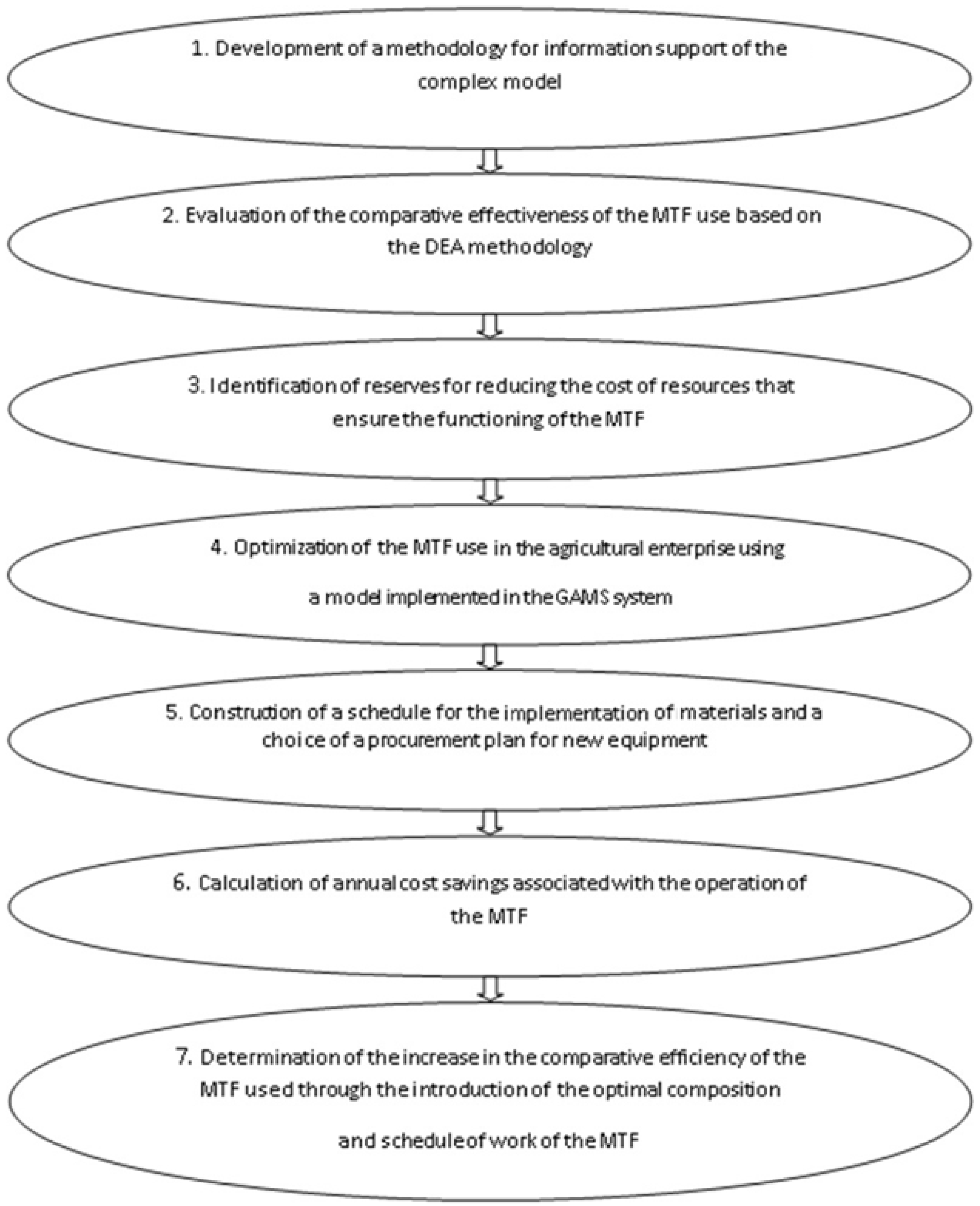
• At the first stage of this method, primary data on the functioning of the MTF of the agricultural enterprise are collected and processed. For example, calculations of the planned production rates and the cost of implementation of the MTF must be carried out. In addition, the permissible values of exogenous variables must be determined. In particular, the agro-terms of mechanized field work, and the available number of tractors and combines in the MTF are determined. It should be emphasized that with the exception of one loader and one combine harvester in the agricultural enterprise “Novy Dvor-Agro”, all the machinery and equipment on both farms are fully involved in the production process. Therefore, it is necessary to update the existing equipment in time when 100% wear is reached.
• At the second stage, in order to develop reserves for improving efficiency on the basis of the economic and mathematical models presented above, the composition and structure of the MTF, as well as the schedule of its work during the planning period, are optimized. In the absence of an initial plan in the form of a current schedule for the work of the MTF, a heuristic algorithm for building an initial plan suitable for launching a model complex can be applied at this stage.
• At the third stage, a numerical solution obtained in the GAMS system is brought into the line with the integer requirement and checked for compliance with the constraints of the mathematical model. If necessary, the optimal plan is adjusted.
• At the fourth stage, on the basis of the modified optimal plan, a schedule for the implementation of the MT works for the planning period is constructed.
• The fifth stage consists of a comparison of the total costs for the agricultural operations of the MTF of the enterprise before and after optimization, with a breakdown into separate cost elements. The economic effect of the introduction of the proposed algorithm is estimated.

The developed method for optimizing the formation and use of the MTF of an agricultural enterprise in field cultivation that is proposed within the framework of this study can be successfully applied in managing the agro-industrial complex at the micro-level and meso-level. The process enables decision makers to optimize the schedule of the MTF for a given period, to draw up an optimal plan for the purchase of new equipment in terms of their total costs, and to identify unused equipment. The proposed model and algorithm can improve the comparative efficiency in the use of an enterprise’s MTF. Optimization ensures a reduction in the cost of material resources, resulting in increased profitability of agricultural production.

References

1. Durczak, K.; Ekielski, A.; Kozłowski, R.; Zelazinski, T.; Pilarski, K. A computer system supporting agricultural machinery and farm tractor purchase decisions. Heliyon 2020, 6, e05039. [Google Scholar] [CrossRef] [PubMed]
2. Gorodov, A.A.; Gorodova, L.V.; Fedorova, M.A. Optimizing the use of the machine and tractor fleet of an agricultural enterprise. J. Krasn. State Agric. Univ. 2014, 9, 3–11. (In Russian) [Google Scholar]
3. Vazquez, D.A.Z.; Fan, N.; Teegerstrom, T.; Seavert, C.; Summers, H.M.; Sproul, E.; Quinn, J.C. Optimal production planning and machinery scheduling for semi-arid farms. Comput. Electron. Agric. 2021, 187, 106288. [Google Scholar] [CrossRef]
4. Capitanescu, F.; Marvuglia, A.; Gutierrez, T.N.; Benetto, E. Multi-stage farm management optimization under environmental and crop rotation constraints. J. Clean. Prod. 2017, 147, 197–205. [Google Scholar] [CrossRef]
5. Pazova, T.H.; Shekihachev, Y.A.; Sohrokov, A.H. Optimization of the set of machine and tractors fleet. Polythematic Online Electron. Sci. J. Kuban State Agrar. Univ. 2012, 75, 113–116. (In Russian) [Google Scholar]
6. Kusnharev, L.I.; Dzuganov, V.B.; Dzuganov, A.V. Results of optimization of the machine-tractor park of farms and machine-technological stations. Int. Sci. J. 2013, 4, 13–18. (In Russian) [Google Scholar]
7. Toba, A.-L.; Griffel, L.M.; Hartley, D.S. Devs based modeling and simulation of agricultural machinery movement. Comput. Electron. Agric. 2020, 177, 105669. [Google Scholar] [CrossRef]
8. Li, J.; Li, T.; Yu, Y.; Zhang, Z.; Pardalos, P.M.; Zhang, Y.; Ma, Y. Discrete firefly algorithm with compound neighborhoods for asymmetric multi-depot vehicle routing problem in the maintenance of farm machinery. Appl. Soft Comput. J. 2019, 81, 105460. [Google Scholar] [CrossRef]
9. Hafezalkotob, A.; Hami-Dindar, A.; Rabie, N.; Hafezalkotob, A. A decision support system for agricultural machines and equipment selection: A case study on olive harvester machines. Comput. Electron. Agric. 2018, 148, 207–216. [Google Scholar] [CrossRef]
10. Camarena, E.A.; Gracia, C.; Sixto, J.M.; Cabrera, A. Mixed integer linear programming machinery selection model for multifarm systems. Biosyst. Eng. 2004, 87, 145–154. [Google Scholar] [CrossRef]
11. Bochtis, D.D.; Sorensen, C.G.C.; Busato, P. Advances in agricultural machinery management: A review. Biosyst. Eng. 2014, 126, 69–81. [Google Scholar] [CrossRef]
12. Ahma, U.; Sharm, L. A review of best management practices for potato crop using precision agricultural technologies. Smart Agric. Technol. 2023, 4, 100220. [Google Scholar] [CrossRef]
13. Cao, R.; Li, S.; Ji, Y.; Zhang, Z.; Xu, H.; Zhang, M.; Li, M.; Li, H.; Zhou, J. Task assignment of multiple agricultural machinery cooperation based on improved ant colony algorithm. Comput. Electron. Agric. 2021, 182, 105993. [Google Scholar] [CrossRef]
14. Cao, R.; Guo, Y.; Zhang, Z.; Li, S.; Zhang, M.; Li, H.; Li, M. Global path conflict detection algorithm of multiple agricultural machinery cooperation based on topographic map and time window. Comput. Electron. Agric. 2023, 208, 107773. [Google Scholar] [CrossRef]
15. Wang, Y.-J.; Huang, G.Q. A two-step framework for dispatching shared agricultural machinery with time windows. Comput. Electron. Agric. 2022, 192, 106607. [Google Scholar] [CrossRef]
16. Volkova, E.; Smolyaninova, N. Trends in Russian exports and imports of agricultural machinery. Transp. Res. Procedia 2022, 63, 1131–1138. [Google Scholar] [CrossRef]
17. Han, J.; Xiang, Q.; Zeng, B.; Lei, Y.; Luo, L. A multi-objective dynamic covering location problem for hierarchical agricultural machinery maintenance facilities. Knowl.-Based Syst. 2022, 252, 109462. [Google Scholar] [CrossRef]
18. Hu, Y.; Liu, Y.; Wang, Z.; Wen, J.; Li, J.; Lu, J. A two-stage dynamic capacity planning approach for agricultural machinery maintenance service with demand uncertainty. Biosyst. Eng. 2020, 190, 201–217. [Google Scholar] [CrossRef]
19. Han, J.; Zhang, J.; Zeng, B.; Mao, M. Optimizing dynamic facility location-allocation for agricultural machinery maintenance using Benders decomposition. Omega 2021, 105, 102498. [Google Scholar] [CrossRef]
20. Cupial, M.; Szeląg-Sikora, A.; Niemiec, M. Optimisation of the machinery park with the use of OTR-7 software in context of sustainable agriculture. Agric. Agric. Sci. Procedia 2015, 7, 64–69. [Google Scholar] [CrossRef]
21. Bang-Jensen, J.; Gutin, G.; Yeo, A. When the greedy algorithm fails. Discret. Optim. 2004, 1, 121–127. [Google Scholar] [CrossRef]
22. Werner, F.; Burtseva, L.; Sotskov, Y.N. Special issue on algorithms for scheduling problems. Algorithms 2018, 11, 87. [Google Scholar] [CrossRef]
23. Werner, F.; Burtseva, L.; Sotskov, Y.N. Special issue on exact and heuristic scheduling algorithms. Algorithms 2020, 13, 9. [Google Scholar] [CrossRef]
Disclaimer/Publisher’s Note: The statements, opinions and data contained in all publications are solely those of the individual author(s) and contributor(s) and not of MDPI and/or the editor(s). MDPI and/or the editor(s) disclaim responsibility for any injury to people or property resulting from any ideas, methods, instructions or products referred to in the content.
Article Metrics
Citations
Article Access Statistics
Multiple requests from the same IP address are counted as one view.