Implementing Deep Convolutional Neural Networks for QR Code-Based Printed Source Identification
Abstract
1. Introduction
- A comparison is conducted of the identification accuracy of seven popular pretrained CNN models using three different optimizers on separate BW and color QR code datasets to identify the printed sources.
- To identify which printers are the easiest and most difficult to distinguish among our printer datasets, we compared the performance of seven popular pretrained CNN models using three different optimizers.
- We analyzed how each pretrained model behaves differently with BW and color QR code datasets.
- A customized CNN is designed and developed to identify printed sources based on a residual model. The network has a small number of parameters and is designed to be fast and reliable with a tweakable input size, convolution kernel size, and hyperparameters.
2. Related Work
2.1. Texture-Based Methods
2.2. Deep Learning-Based Methods
2.3. Quick Response (QR) Code
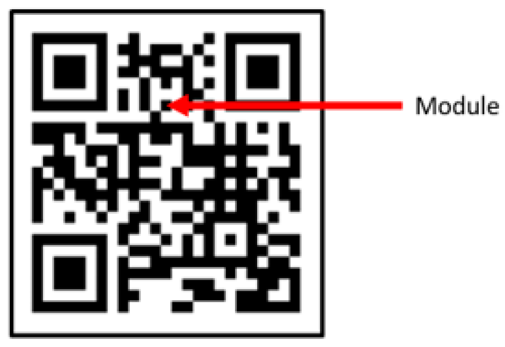
- Level L (Low) 7% of codewords can be restored;
- Level M (Medium) 15% of codewords can be restored;
- Level Q (Quartile) 25% of codewords can be restored;
- Level H (High) 30% of codewords can be restored.
2.3.1. Non-Data (Also Known as Functional Patterns)
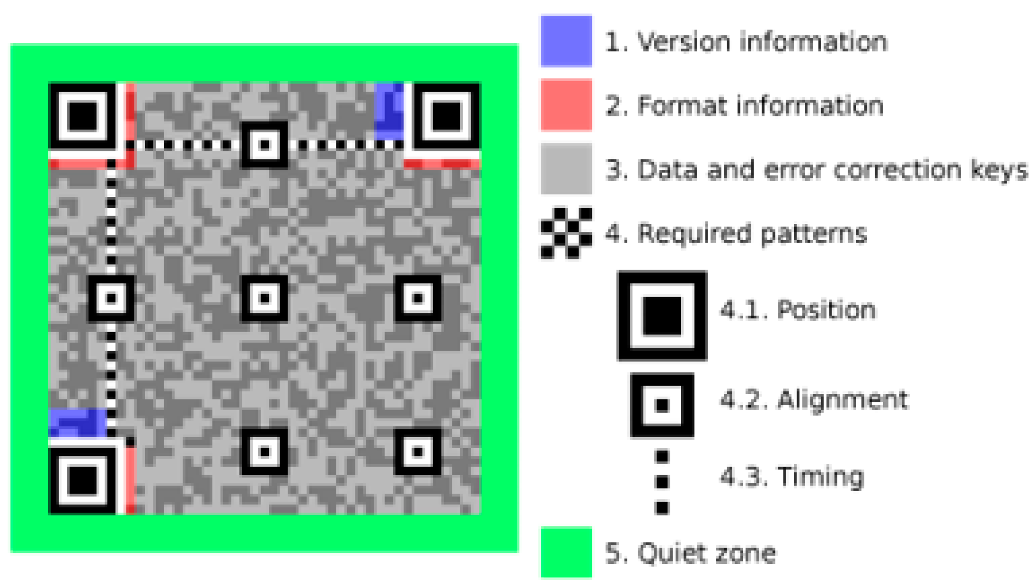
- The positioning pattern is a crucial feature of the QR code. It consists of three large black-and-white concentric squares located in the upper left and right and lower left. Losing one of these patterns greatly affects recognition, as they are essential for QR code recognition.
- The separator pattern is a continuous white-coded element that surrounds the positioning pattern to distinguish it from other regions.
- The timing pattern is a ribbon of alternating black and white code elements that is barely noticeable as it blends in with the other blocks of codewords. It appears in all versions of QR codes and is also known as the “fixed pattern” due to its fixed alternating pattern and position. The timing pattern consists of two straight lines that confirm the size of the code element.
- The alignment pattern, also known as the alignment marker, is only found in QR code version 1. The other versions require the addition of an alignment pattern for positioning. If the alignment pattern is too large, it can be easily deformed during scanning. However, the alignment pattern can be used as a reference to correct the deformation of the QR code.
2.3.2. Data Codeword Filling Method
2.4. Development of Color QR Code for Visual Beautification
2.5. Convolutional Neural Networks
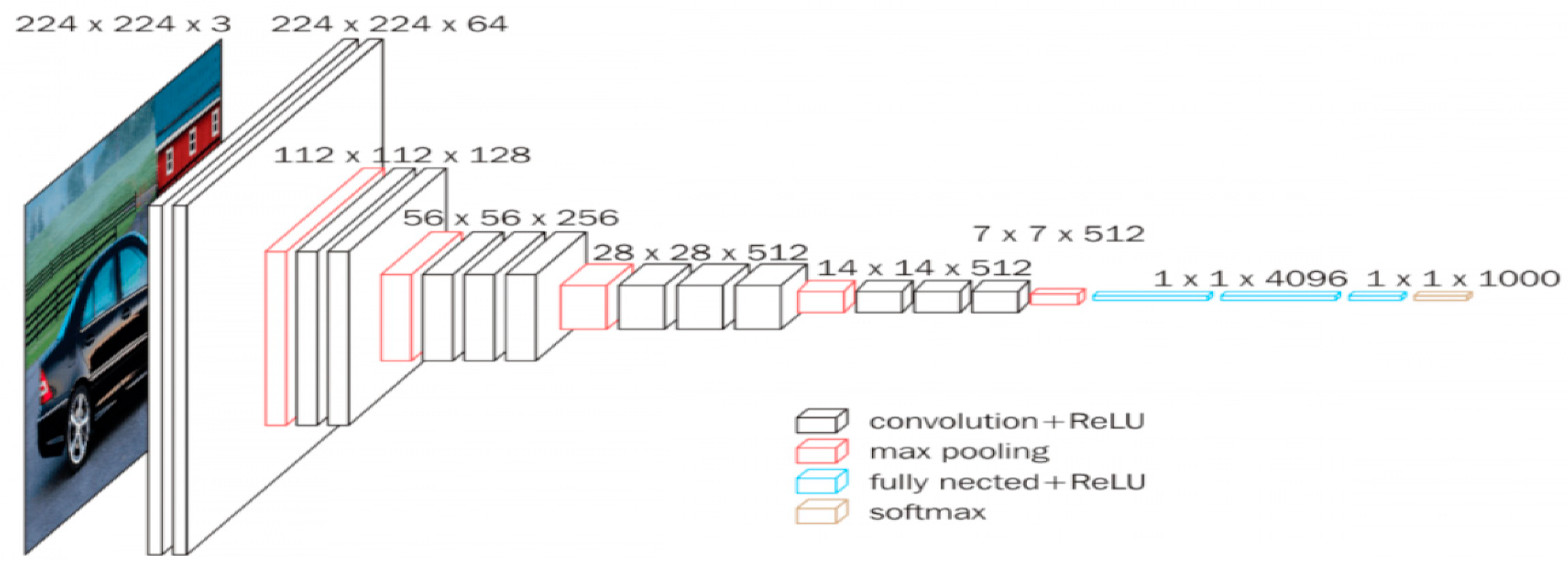
- Input layer: This is where the data are fed into the network. The input data, which can be either raw image pixels or their transformations, are fed into the network at the beginning. These data can be selected to better emphasize specific aspects of the image.
- Convolutional layers: These layers contain a series of fixed-size filters used to perform convolution on the image data, generating a so-called feature map. These filters can highlight patterns such as edges and changes in color, which help characterize the image.
- Rectified Linear Unit (ReLU): ReLU layers, which normally follow a convolution operation, apply a non-linear function to the output x of the previous layer, such as f(x) = max(0,x). According to Krizhevsky et al. [20], this function can be computed faster than its equivalents with tanh units in terms of training time with gradient descent. This helps to create rapid convergence in the training process by reducing the vanishing gradient problem and more or less maintaining the constancy of the gradient in all the network layers, thereby speeding up the training process.
- Pooling layers: A pooling layer summarizes the data by applying some linear or non-linear operation, such as generalized mean or max, to the data within a window that slides across the feature maps. This reduces the spatial size of the feature maps used by the subsequent layers and helps the network to focus only on the most important patterns identified by the convolutional layers and ReLU, thereby minimizing computation intensity.
- Fully connected layers: The fully connected layers are located at the end of the network and are used for understanding the patterns generated by the previous layers. They act as classifiers, usually followed by a soft-max layer to determine the class associated with the input image.
- Soft-max layer: The soft-max layer is typically used during training at the network’s end. It normalizes the input values so that they add up to one, and its output can be interpreted as a probability distribution, such as the probability of a sample belonging to each class.
3. Proposed Method
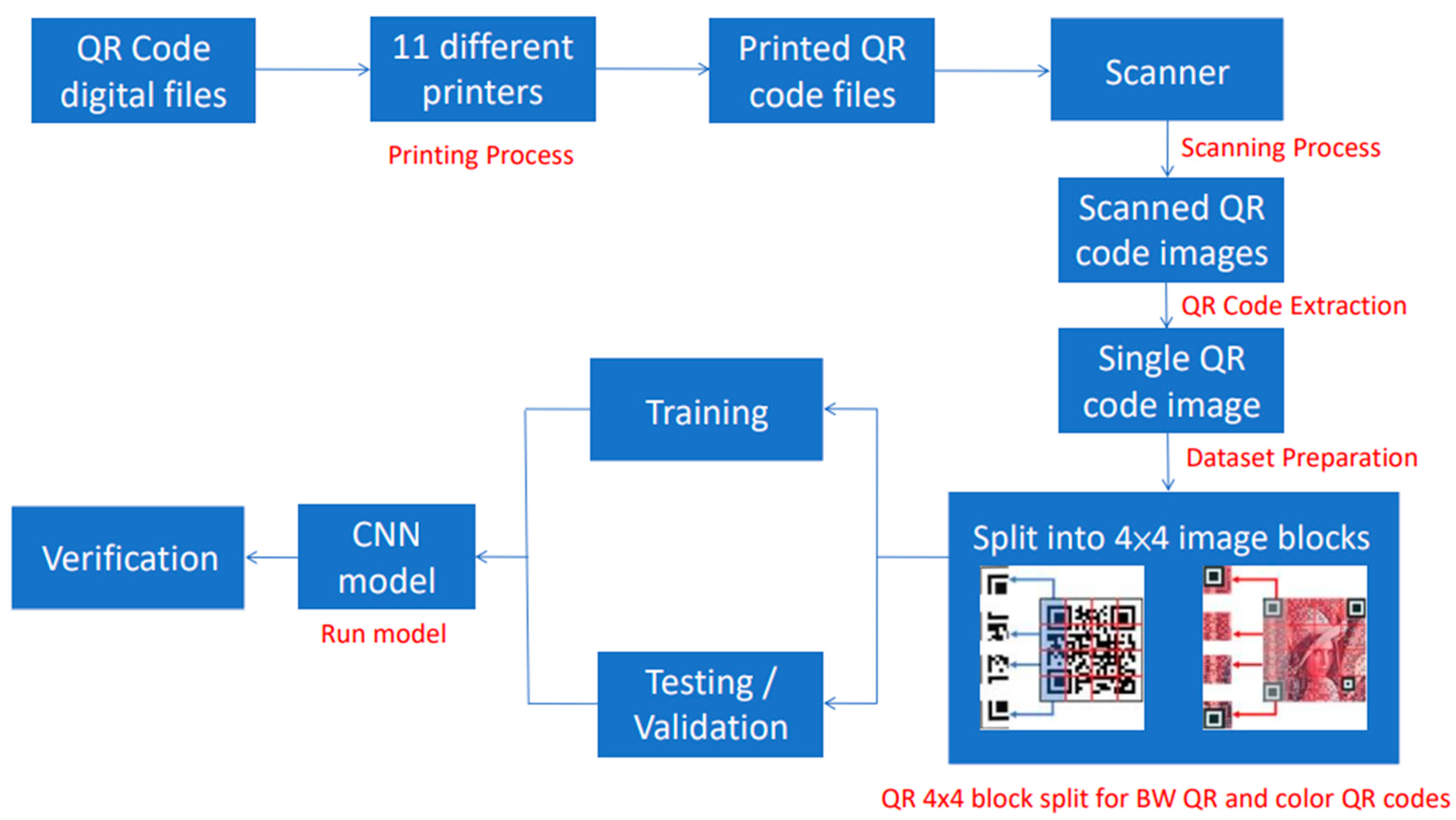
- Printing Process:
- Scanning Process: The printed QR codes are digitalized using a dedicated office scanner, and all the documents are saved in TIF lossless image format. BW QR code uses 8-bit grayscale format, while color QR code is saved in 24-bit RGB format.
- QR code extraction: Using MATLAB, the regionprops and imcrop functions are combined to automatically crop and resize all 24 QR codes on one page. This process is looped 24 times from the top left to right.
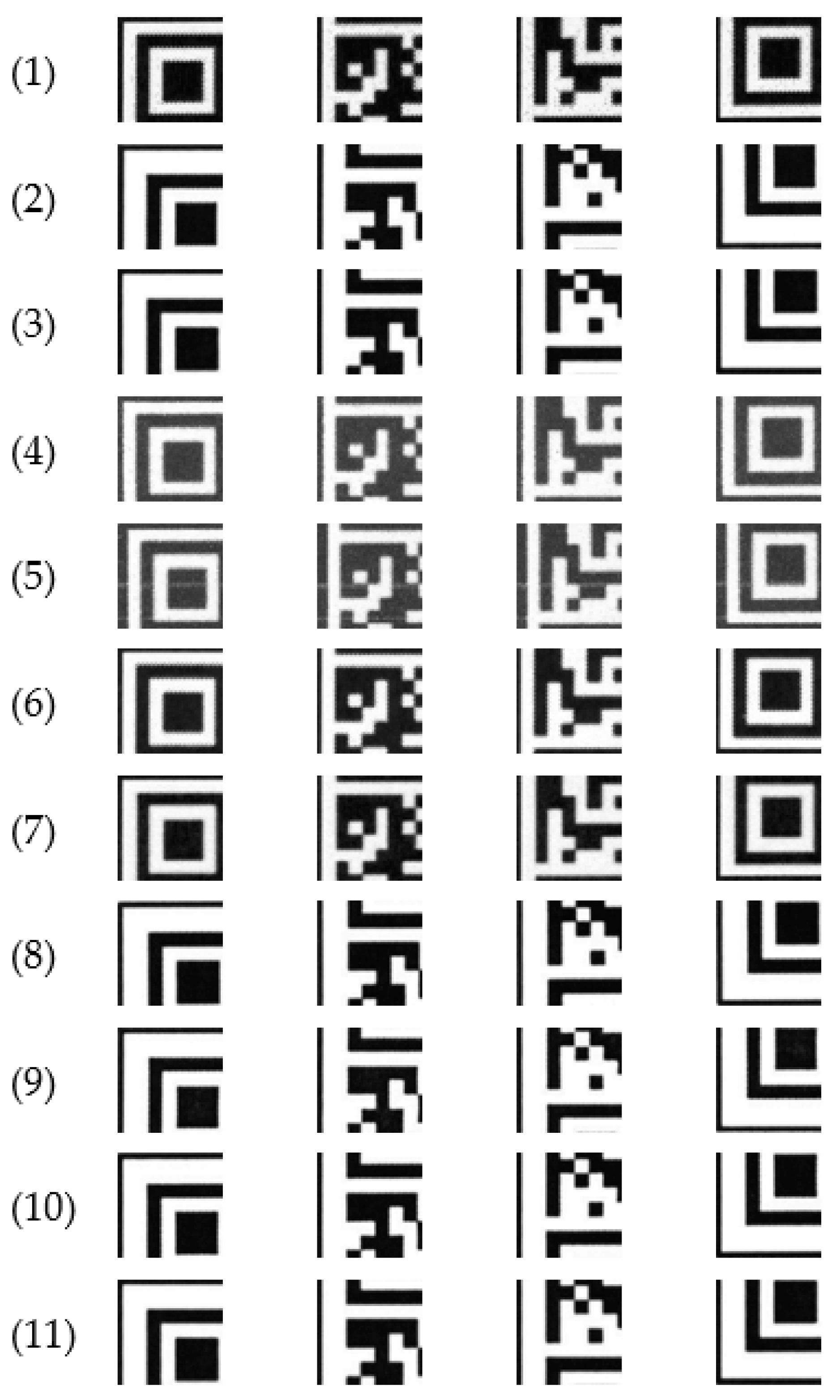
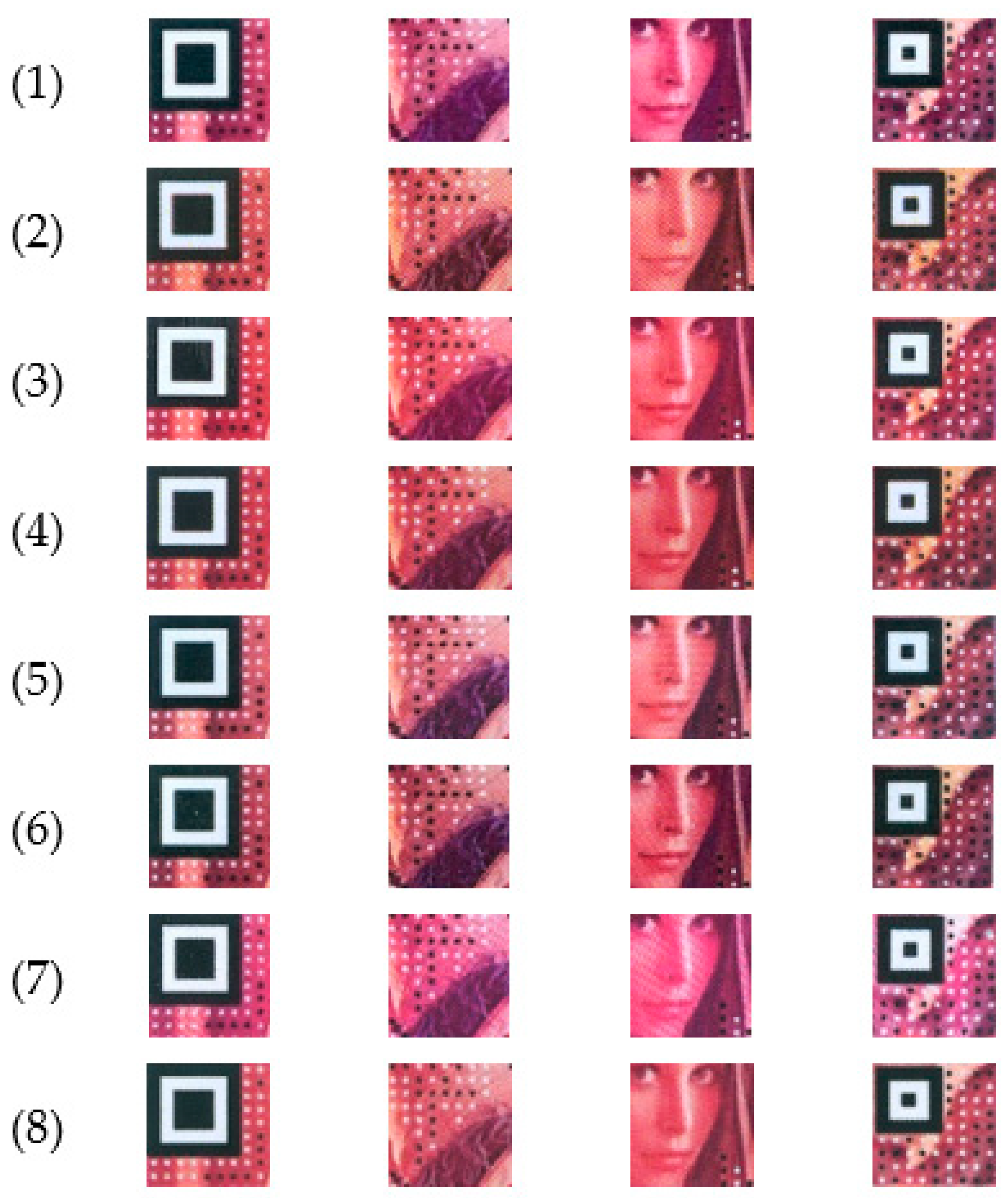
- Dataset preparation: An open-source image viewer, XnView MP, is implemented to divide all extracted QR codes into 4 × 4 image blocks by batch. Moreover, all BW QR code images are converted from 8-bit format to 24-bit format, as required by the pretrained models. The cropping process does not affect the image quality because the image is neither reconstructed nor resized.
- Run model: The CNN model is operated to put a new set of images into categories.
3.1. Data Collection
- BW QR codes: 2640 QR codes are collected after printing the documents with 11 individual printers (Table 1).
- Color QR codes: to compare the same model with BW QR codes, documents are printed with 8 printer models, resulting in 1920 color QR codes collected in total.
3.2. QR Code Extraction
4. Experimental Results
4.1. Training Environment
4.2. Performance Evaluation of BW QR Codes
Performance Evaluation for Color QR Codes
4.3. Customized Fine-Tuned Residual Model Structure
4.3.1. Defining the Network Architecture: The Components of the Residual Network Architecture
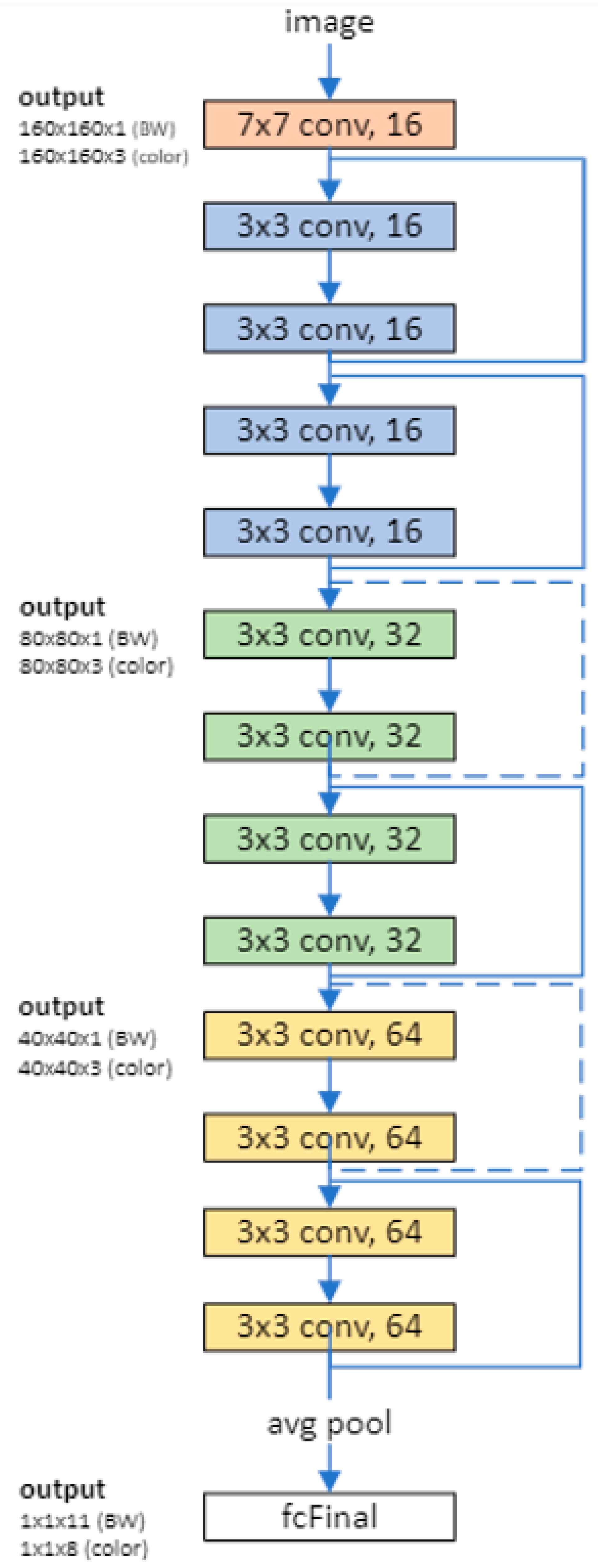
- The key branch of the network is divided into various twisting layers with batch normalization and ReLU activation functions that are connected consecutively.
- The network has residual connections that bypass the convolutional units in the main branch. An element adds the outputs of the residual connections and convolutional units. The residual connections must also include 1-by-1 convolutional layers when the activation size differs. In addition, they will allow the parameter gradients to more easily propagate from the output layer to the earlier layers of the network, enabling training networks.
4.3.2. Creating the Main Branch of the Network with Five Sections
- The network begins with an initial section that includes the image input layer and an initial convolution with activation.
- The network has three stages of convolutional layers with different feature sizes (160-by-160, 80-by-80, and 40-by-40) and different kernel sizes (7 × 7, 5 × 5, and 3 × 3) in the first convolution layer. Each stage includes N convolutional units. In this example, N = 2. Each convolutional unit contains two 3-by-3 convolutional layers with activations. The net width parameter shows the network defined as the number of filters in the convolutional layers in the first stage of the network. The first convolutional units in the second and third stages down-sample the spatial dimensions by a factor of two. The number of filters is accumulated by a factor of two each time spatial down-sampling is performed in order to maintain approximately the same amount of computation in each individual convolutional layer throughout the network.
- The final section of the network includes global average pooling, fully connected, softmax, and classification layers.
4.4. Performance Evaluation of Customized Fine-Tuned Residual Model
5. Conclusions and Future Work
5.1. Conclusions
5.2. Future Works
Author Contributions
Funding
Institutional Review Board Statement
Informed Consent Statement
Data Availability Statement
Acknowledgments
Conflicts of Interest
References
- Zhu, B.; Wu, J.; Kankanhalli, M.S. Print signatures for document authentication. In Proceedings of the 10th ACM Conference on Computer and Communications Security (CCS), Washington, DC, USA, 27–30 October 2003; pp. 145–154. [Google Scholar]
- Chiang, P.J.; Khanna, N.; Mikkilineni, A.K.; Segovia, M.V.O.; Suh, S.; Allebach, J.P.; Chiu, G.T.-C.; Delp, E.J. Printer and scanner forensics. IEEE Signal Process. Mag. 2009, 26, 72–83. [Google Scholar] [CrossRef]
- Cicconi, F.; Lazic, V.; Palucci, A.; Assis, A.C.A.; Saverio Romolo, F. Forensic analysis of Commercial Inks by Laser-Induced Breakdown Spectroscopy (LIBS). Sensors 2020, 20, 3744. [Google Scholar] [CrossRef] [PubMed]
- ABraz; Lopez-Lopez, M.; Garcia-Ruiz, C. Raman spectroscopy for forensic analysis of inks in questioned documents. Forensic Sci. Int. 2013, 232, 206–212. [Google Scholar]
- Gal, L.; Belovicova, M.; Oravec, M.; Palkova, M.; Ceppan, M. Analysis of laser and inkjet prints using spectroscopic methods for forensic identification of questioned documents. Symp. Graph. Arts 1993, 10, 1–8. [Google Scholar]
- Chu, P.-C.; Cai, B.; Tsoi, Y.; Yuen, R.; Leung, K.; Cheung, N.-H. Forensic analysis of laser printed ink by x-ray fluorescence and laser-excited plume fluorescence. Anal. Chem. 2013, 85, 4311–4315. [Google Scholar] [CrossRef]
- Barni, M.; Podilchuk, C.I.; Bartolini, F.; Delp, E.J. Watermark embedding: Hiding a signal within a cover image. IEEE Commun. Mag. 2001, 39, 102–108. [Google Scholar] [CrossRef]
- Fu, M.S.; Au, O. Data hiding in halftone images by stochastic error diffusion. In Proceedings of the IEEE International Conference Acoustics, Speech, and Signal Processing, 2001, (ICASSP 01), Salt Lake City, UT, USA, 7–11 May 2001; Volume 3, pp. 1965–1968. [Google Scholar]
- Bulan, O.; Monga, V.; Sharma, G.; Oztan, B. Data embedding in hardcopy images via halftone-dot orientation modulation. In Proceedings of the Security, Forensics, Steganography, and Watermarking of Multimedia Contents X, San Jose, CA, USA, 27–31 January 2008; Volume 6819, p. 68190C-1-12. [Google Scholar]
- Kim, D.-G.; Lee, H.-K. Colour laser printer identification using halftone texture fingerprint. Electron. Lett. 2015, 51, 981–983. [Google Scholar] [CrossRef]
- Ferreira, A.; Bondi, L.; Baroffio, L.; Bestagini, P.; Huang, J.; Dos Santos, J.A.; Tubaro, S.; Rocha, A.D.R. Data-driven feature characterization techniques for laser printer attribution. IEEE Trans. Inf. Forensics Secur. 2017, 12, 1860–1872. [Google Scholar] [CrossRef]
- Mikkilineni, A.K.; Chiang, P.-J.; Ali, G.N.; Chiu, G.T.-C.; Allebach, J.P.; Delp, E.J. Printer identification based on textural features. In Proceedings of the International Conference on Digitial Printing Technologies, West Lafayette, IN, USA, 18–23 October 2004; pp. 306–311. [Google Scholar]
- Mikkilineni, A.K.; Arslan, O.; Chiang, P.J.; Kumontoy, R.M.; Allebach, J.P.; Chiu, G.T.; Delp, E.J. Printer forensics using SVM techniques. In Proceedings of the International Conference on Digitial Printing Technologies, Baltimore, MD, USA, 18–23 September 2005; pp. 223–226. [Google Scholar]
- Mikkilineni, K.A.; Chiang, P.-J.; Ali, G.N.; Chiu, G.T.C.; Allebach, J.P.; Delp, E.J. Printer identification based on graylevel co-occurrence features for security and forensic applications. In Proceedings of the SPIE International Conference on Security, Steganography, and Watermarking of Multimedia Contents VII, San Jose, CA, USA, 17–20 January 2005; Volume 5681, pp. 430–441. [Google Scholar]
- Ferreira, A.; Navarro, L.C.; Pinheiro, G.; dos Santos, J.A.; Rocha, A. Laser printer attribution: Exploring new features and beyond. Forensic Sci. Int. 2015, 247, 105–125. [Google Scholar] [CrossRef]
- Tsai, M.-J.; Yuadi, I.; Tao, Y.-H. Decision-theoretic model to identify printed sources. Multimed. Tools Appl. 2018, 77, 27543–27587. [Google Scholar] [CrossRef]
- Joshi, S.; Khanna, N. Single classifier-based passive system for source printer classification using local texture features. IEEE Trans. Inf. Forensics Secur. 2018, 13, 1603–1614. [Google Scholar] [CrossRef]
- Tsai, M.-J.; Yin, J.-S.; Yuadi, I.; Liu, J. Digital forensics of printed source identification for Chinese characters. Multimed. Tools Appl. 2014, 73, 2129–2155. [Google Scholar] [CrossRef]
- LeCunn, Y.; Bengio, Y.; Hinton, G. Deep learning. Nature 2015, 521, 436–444. [Google Scholar] [CrossRef] [PubMed]
- Krizhevsky, A.; Sutskever, I.; Hinton, G.E. ImageNet classification with deep convolutional neural networks. Commun. ACM 2017, 60, 84–90. [Google Scholar] [CrossRef]
- Kim, D.-G.; Hou, J.-U.; Lee, H.-K. Learning deep features for source color laser printer identification based on cascaded learning. Neurocomputing 2019, 365, 219–228. [Google Scholar] [CrossRef]
- Guo, Z.-Y.; Zheng, H.; You, C.-H.; Xu, X.-H.; Wu, X.-B.; Zheng, Z.-H.; Ju, J.-P. Digital forensics of scanned QR code images for printer source identification using bottleneck residual block. Sensors 2020, 20, 6305. [Google Scholar] [CrossRef]
- QR Code. Available online: https://en.wikipedia.org/wiki/QR_code#/media/File:QR_Code_Structure_Example_3.svg (accessed on 6 January 2022).
- Chu, H.-K.; Chang, C.-S.; Lee, R.-R.; Mitra, N.J. Halftone QR codes. ACM Trans. Graph. 2013, 32, 217. [Google Scholar] [CrossRef]
- Garateguy, G.J.; Arce, G.R.; Lau, D.L.; Villarreal, O.P. QR Images: Optimized Image Embedding in QR Codes. IEEE Trans. Image Process. 2014, 23, 2842–2853. [Google Scholar] [CrossRef]
- Li, L.; Qiu, J.; Lu, J.; Chang, C.-C. An aesthetic QR code solution based on error correction mechanism. J. Syst. Softw. 2016, 116, 85–94. [Google Scholar] [CrossRef]
- Lin, L.; Wu, S.; Liu, S.; Jiang, B. Interactive QR code beautification with full background image embedding. In Proceedings of the SPIE International Conference on Second International Workshop on Pattern Recognition, Singapore, 1–3 May 2017; Volume 10443, p. 1044317. [Google Scholar]
- Lin, L.; Zou, X.; He, L.; Liu, S.; Jiang, B. Aesthetic QR code generation with background contrast enhancement and user interaction. In Proceedings of the SPIE International Conference on Third International Workshop on Pattern Recognition, Jinan, China, 26–28 May 2018; p. 108280G. [Google Scholar]
- Tsai, M.-J.; Hsieh, C.-Y. The visual color QR code algorithm (DWT-QR) based on wavelet transform and human vision system. Multimed. Tools Appl. 2019, 78, 21423–21454. [Google Scholar] [CrossRef]
- Tsai, M.-J.; Lin, D.-T. QR Code Beautification by Deep Learning Technology. Master’s Thesis, National Yang Ming Chiao Tung University, Hsinchu, Taiwan, 2021. [Google Scholar]
- Do, T.-N. Incremental and parallel proximal SVM algorithm tailored on the Jetson Nano for the ImageNet challenge. Int. J. Web Inf. Syst. 2022, 18, 137–155. [Google Scholar] [CrossRef]
- Tsai, M.-J.; Peng, S.-L. QR code beautification by instance segmentation (IS-QR). Digit. Signal Process. 2022, 133, 103887. [Google Scholar] [CrossRef]
- Wang, Z.; Zuo, C. Zeng. SAE based unified double JPEG compression detection system for Web image forensics. Int. J. Web Inf. Syst. 2021, 17, 84–98. [Google Scholar] [CrossRef]
- Tsai, M.-J.; Wu, H.-U.; Lin, D.T. Auto ROI & mask R-CNN model for QR code beautification (ARM-QR). Multimed. Syst. 2023. [Google Scholar] [CrossRef]
- Lecun, Y.; Bottou, L.; Bengio, Y.; Haffner, P. Gradient-based learning applied to document recognition. Proc. IEEE 1998, 86, 2278–2324. [Google Scholar] [CrossRef]
- Transfer Learning in Keras Using VGG16. 2020. Available online: https://thebinarynotes.com/transfer-learning-keras-vgg16/ (accessed on 7 February 2022).
| No | Brand | Model |
|---|---|---|
| 1 | Canon | LBP3310 |
| 2 | Canon | LBP6300 |
| 3 | Canon | M417 LIPSX |
| 4 | Epson | L350 |
| 5 | Epson | L3110 |
| 6 | Fuji Xerox | P355d |
| 7 | HP | M283 |
| 8 | HP | M377 |
| 9 | HP | M401 |
| 10 | HP | M425 |
| 11 | Konica Minolta | Bizhub C364 |
| No | Brand | Model |
|---|---|---|
| 1 | Canon | ImageRunner 6555i |
| 2 | Canon | LBP9200C |
| 3 | Fuji Xerox | ApeosPort-VII |
| 4 | Fuji Xerox | DocuCentre-IV |
| 5 | HP | M283 |
| 6 | HP | M377 |
| 7 | Konica Minolta | Magicolor 1690 |
| 8 | Kyocera | Ecosys M5520 |
| Parameter | Value/Type |
|---|---|
| Image Size | 160 × 160, 224 × 224, 227 × 227 |
| Cross Validation | Holdout |
| Training/Testing | 80/20 |
| Optimizer | SGDM, ADAM, RMSprop |
| Max Epochs | 30 |
| Minibatch Size | 64 |
| Shuffle | Every epoch |
| Initial Learn Rate | 10−3 no decay |
| Augmentation Type | Purpose | Value |
|---|---|---|
| RandXReflection | Reflection in the left-right direction randomly appears, specified as a logical scalar. The image is reflected horizontally with a 50% probability | 1 (true) |
| RandXTranslation | Moving the image in the X or Y direction (or both) from the center coordinate. This forces the convolutional neural network to look everywhere within the image dimension. | [−30, 30] |
| RandYTranslation | ||
| RandXScale | The image is scaled outward or inward. While scaling outward, the final image size is larger than the original. Most image frameworks cut out a section from the new image, with a size equal to the original image. Scaling inward reduces the image size, forcing the model to make assumptions about what lies beyond the boundary. | [0.9, 1.1] |
| RandYScale |
| Model Name | Optimizer | Accuracy (%) | Precision | Recall | Specificity | Train Time (min) |
|---|---|---|---|---|---|---|
| AlexNet | SGDM | 97.7 | 0.98 | 0.98 | 0.99 | 143 |
| Adam | 9.09 | 0.01 | 0.09 | 0.91 | -- | |
| RMSprop | 9.09 | 0.01 | 0.09 | 0.91 | -- | |
| GoogleNet | SGDM | 98.3 | 0.98 | 0.98 | 0.99 | 65 |
| Adam | 89.8 | 0.94 | 0.90 | 0.99 | 68 | |
| RMSprop | 84.2 | 0.86 | 0.84 | 0.98 | 66 | |
| DenseNet201 | SGDM | 99.7 | 0.99 | 0.99 | 1.00 | 839 |
| Adam | 97.8 | 0.98 | 0.98 | 0.99 | 1090 | |
| RMSprop | 97.8 | 0.98 | 0.98 | 0.99 | 984 | |
| MobileNetv2 | SGDM | 99.7 | 0.99 | 0.99 | 0.99 | 117 |
| Adam | 99.3 | 0.99 | 0.99 | 0.99 | 151 | |
| RMSprop | 99.7 | 0.99 | 0.99 | 1.00 | 136 | |
| ResNet18 | SGDM | 99.9 | 0.99 | 0.99 | 1.00 | 53 |
| Adam | 99.4 | 0.99 | 0.99 | 0.99 | 55 | |
| RMSprop | 99.4 | 0.99 | 0.99 | 0.99 | 49 | |
| ResNet50 | SGDM | 99.9 | 1.00 | 1.00 | 1.00 | 108 |
| Adam | 99.5 | 0.99 | 0.99 | 0.99 | 124 | |
| RMSprop | 99.5 | 0.99 | 0.99 | 0.99 | 121 | |
| VGG16 | SGDM | 99.6 | 0.99 | 0.99 | 1.00 | 114 |
| Adam | 9.09 | 0.01 | 0.09 | 0.91 | -- | |
| RMSprop | 9.09 | 0.01 | 0.09 | 0.91 | -- | |
| Our Model | SGDM | 99.7 | 0.99 | 0.99 | 1.00 | 51 |
| Adam | 99.7 | 0.99 | 0.99 | 1.00 | 59 | |
| RMSprop | 99.8 | 0.99 | 0.99 | 1.00 | 55 |
| Model Name | Optimizer | Accuracy | 1 | 2 | 3 | 4 | 5 | 6 | 7 | 8 | 9 | 10 | 11 |
|---|---|---|---|---|---|---|---|---|---|---|---|---|---|
| Alex Net | SGDM | 0.9770 | 0.882 | 1 | 1 | 1 | 1 | 0.973 | 0.991 | 1 | 0.995 | 0.987 | 0.921 |
| Adam | 0.9090 | -- | -- | -- | -- | -- | -- | -- | -- | -- | -- | -- | |
| RMSprop | 0.9090 | -- | -- | -- | -- | -- | -- | -- | -- | -- | -- | -- | |
| Google Net | SGDM | 0.9828 | 0.986 | 1 | 1 | 1 | 0.997 | 1 | 0.995 | 0.978 | 1 | 0.910 | 0.945 |
| Adam | 0.8981 | 0.936 | 0.943 | 1 | 1 | 1 | 1 | 0.997 | 0.992 | 0.995 | 0.829 | 0.186 | |
| RMSprop | 0.8420 | 0.984 | 0.913 | 0.839 | 0.785 | 1 | 1 | 0.913 | 0.855 | 0.931 | 0.727 | 0.315 | |
| Dense Net201 | SGDM | 0.9969 | 1 | 1 | 1 | 0.999 | 1 | 1 | 1 | 0.992 | 1 | 0.975 | 1 |
| Adam | 0.9776 | 0.954 | 0.984 | 1 | 1 | 1 | 1 | 0.990 | 0.842 | 0.996 | 1 | 0.987 | |
| RMSprop | 0.9776 | 0.958 | 0.997 | 1 | 1 | 1 | 1 | 1 | 0.801 | 0.997 | 1 | 1 | |
| Mobile Netv2 | SGDM | 0.9978 | 1 | 1 | 1 | 1 | 1 | 0.995 | 0.995 | 0.997 | 1 | 0.999 | 0.990 |
| Adam | 0.9928 | 0.930 | 1 | 1 | 1 | 1 | 1 | 1 | 0.997 | 0.995 | 0.999 | 1 | |
| RMSprop | 0.9966 | 0.999 | 1 | 1 | 1 | 1 | 1 | 1 | 1 | 0.964 | 1 | 1 | |
| Res Net18 | SGDM | 0.9987 | 0.995 | 1 | 1 | 1 | 1 | 1 | 0.997 | 0.999 | 1 | 0.997 | 0.997 |
| Adam | 0.9943 | 1 | 0.999 | 0.969 | 1 | 1 | 0.995 | 0.987 | 0.993 | 0.996 | 1 | 0.999 | |
| RMSprop | 0.9944 | 0.986 | 1 | 0.999 | 1 | 1 | 0.987 | 0.996 | 0.995 | 0.987 | 0.990 | 1 | |
| Res Net50 | SGDM | 0.9996 | 1 | 1 | 1 | 1 | 1 | 1 | 1 | 1 | 1 | 1 | 0.996 |
| Adam | 0.9947 | 0.996 | 1 | 0.993 | 1 | 1 | 0.974 | 0.996 | 0.995 | 0.992 | 0.999 | 0.996 | |
| RMSprop | 0.9946 | 0.987 | 0.999 | 0.995 | 1 | 1 | 0.986 | 0.993 | 0.995 | 0.993 | 0.996 | 0.996 | |
| VGG 16 | SGDM | 0.9960 | 1 | 1 | 1 | 1 | 1 | 1 | 1 | 0.999 | 1 | 0.978 | 0.979 |
| Adam | 0.0909 | -- | -- | -- | -- | -- | -- | -- | -- | -- | -- | -- | |
| RMSprop | 0.0909 | -- | -- | -- | -- | -- | -- | -- | -- | -- | -- | -- | |
| Printer Identification Results | 0.976 | 0.990 | 0.988 | 0.987 | 1 | 0.995 | 0.991 | 0.967 | 0.991 | 0.964 | 0.900 | ||
| Model Name | Optimizer | Accuracy (%) | Precision | Recall | Specificity | Train Time (min) |
|---|---|---|---|---|---|---|
| AlexNet | SGDM | 99.6 | 0.99 | 0.99 | 0.99 | 33 |
| Adam | 12.5 | 0.01 | 0.12 | 0.87 | -- | |
| RMSprop | 12.5 | 0.01 | 0.12 | 0.87 | -- | |
| GoogleNet | SGDM | 73.7 | 0.82 | 0.74 | 0.96 | 50 |
| Adam | 71.9 | 0.83 | 0.72 | 0.96 | 52 | |
| RMSprop | 50.9 | 0.59 | 0.51 | 0.93 | 51 | |
| DenseNet201 | SGDM | 96.7 | 0.97 | 0.97 | 0.99 | 749 |
| Adam | 92.3 | 0.95 | 0.92 | 0.98 | 780 | |
| RMSprop | 90.5 | 0.94 | 0.90 | 0.98 | 718 | |
| MobileNetv2 | SGDM | 96.8 | 0.97 | 0.97 | 0.99 | 100 |
| Adam | 98.6 | 0.98 | 0.98 | 0.99 | 109 | |
| RMSprop | 99.9 | 1 | 1 | 1 | 103 | |
| ResNet18 | SGDM | 97.7 | 0.98 | 0.98 | 0.99 | 42 |
| Adam | 97.4 | 0.98 | 0.97 | 0.99 | 43 | |
| RMSprop | 92.7 | 0.94 | 0.93 | 0.99 | 42 | |
| ResNet50 | SGDM | 95.7 | 0.96 | 0.96 | 0.99 | 81 |
| Adam | 95.8 | 0.96 | 0.96 | 0.99 | 95 | |
| RMSprop | 96.3 | 0.96 | 0.96 | 0.99 | 92 | |
| VGG16 | SGDM | 99.8 | 0.99 | 0.99 | 1 | 86 |
| Adam | 12.5 | 0.01 | 0.12 | 0.87 | -- | |
| RMSprop | 12.5 | 0.01 | 0.12 | 0.87 | -- | |
| Our Model | SGDM | 99.69 | 0.99 | 0.99 | 1 | 40 |
| Adam | 99.7 | 0.99 | 0.99 | 0.99 | 42 | |
| RMSprop | 98.63 | 0.98 | 0.98 | 0.99 | 44 |
| Model Name | Optimizer | Accuracy | 1 | 2 | 3 | 4 | 5 | 6 | 7 | 8 |
|---|---|---|---|---|---|---|---|---|---|---|
| AlexNet | SGDM | 0.9956 | 0.979 | 1 | 1 | 1 | 0.999 | 1 | 1 | 0.987 |
| Adam | 0.125 | -- | -- | -- | -- | -- | -- | -- | -- | |
| RMSprop | 0.125 | -- | -- | -- | -- | -- | -- | -- | -- | |
| GoogleNet | SGDM | 0.7366 | 0.997 | 1 | 0.865 | 0.999 | 0.605 | 0.353 | 1 | 0.669 |
| Adam | 0.7188 | 0.897 | 0.991 | 0.685 | 1 | 0.464 | 0.561 | 1 | 0.145 | |
| RMSprop | 0.5095 | 0.743 | 1 | 0.017 | 0.967 | 0.255 | 0.030 | 0.212 | 0.855 | |
| DenseNet201 | SGDM | 0.9666 | 1 | 1 | 0.996 | 0.988 | 0.913 | 0.910 | 1 | 0.925 |
| Adam | 0.9234 | 1 | 1 | 1 | 1 | 0.943 | 0.991 | 1 | 0.447 | |
| RMSprop | 0.905 | 1 | 1 | 1 | 1 | 0.939 | 0.965 | 1 | 0.328 | |
| MobileNetv2 | SGDM | 0.9685 | 1 | 1 | 1 | 0.969 | 0.936 | 0.996 | 0.996 | 0.995 |
| Adam | 0.9857 | 0.999 | 1 | 1 | 0.887 | 1 | 1 | 1 | 1 | |
| RMSprop | 0.9998 | 1 | 1 | 1 | 1 | 0.999 | 1 | 1 | 1 | |
| ResNet18 | SGDM | 0.9773 | 0.999 | 1 | 0.947 | 1 | 0.879 | 0.996 | 0.997 | 0.999 |
| Adam | 0.9744 | 0.999 | 1 | 0.875 | 1 | 0.960 | 0.962 | 1 | 1 | |
| RMSprop | 0.9268 | 1 | 1 | 0.895 | 0.999 | 0.978 | 0.987 | 1 | 0.551 | |
| ResNet50 | SGDM | 0.9566 | 0.999 | 1 | 0.979 | 0.999 | 0.979 | 0.957 | 0.995 | 0.730 |
| Adam | 0.9584 | 1 | 1 | 1 | 0.951 | 0.751 | 0.999 | 1 | 0.967 | |
| RMSprop | 0.9628 | 0.999 | 1 | 1 | 1 | 0.861 | 0.997 | 1 | 0.832 | |
| VGG16 | SGDM | 0.9977 | 1 | 1 | 1 | 1 | 0.995 | 1 | 0.997 | 0.977 |
| Adam | 0.125 | -- | -- | -- | -- | -- | -- | -- | -- | |
| RMSprop | 0.125 | -- | -- | -- | -- | -- | -- | -- | -- | |
| Printer Identification Results | 0.977 | 0.999 | 0.898 | 0.986 | 0.850 | 0.865 | 0.953 | 0.789 | ||
| Layer Name | Output Size | 14-Layer |
|---|---|---|
| convInp | ||
| S1U1conv_x S1U2conv_x | ||
| S2U1conv_x S2U2conv_x | ||
| S3U1conv_x S3U2conv_x | ||
| globalPool | Average pooling | |
| fcFinal softmax | 11 or 8 fully connected, softmax | |
| classoutput | Output into 11 categories (BW) or 8 categories (color) | |
| (A) BW QR CODE | ||||
| Optimizers | BW | |||
| 3 × 3 | 5 × 5 | 7 × 7 | Time | |
| SGDM | 0.9989 | 0.9930 | 0.9963 | 52 min |
| Adam | 0.9991 | 0.9982 | 0.9970 | 59 min |
| RMSprop | 0.9955 | 0.9640 | 0.9989 | 55 min |
| (B) COLOR QR CODE | ||||
| Optimizers | Color | |||
| 3 × 3 | 5 × 5 | 7 × 7 | Time | |
| SGDM | 0.9865 | 0.9557 | 0.9963 | 40 min |
| Adam | 0.9917 | 0.9991 | 0.9949 | 47 min |
| RMSprop | 0.9998 | 1 | 0.9863 | 44 min |
| (A) BW QR CODE | |||||
| Optimizer | Accuracy | Precision | Recall | Sensitivity | Train Time (min) |
| SGDM | 99.69 | 0.997 | 0.997 | 1 | 51.38 |
| Adam | 99.80 | 0.997 | 0.997 | 1 | 55.75 |
| RMSprop | 99.89 | 0.999 | 0.999 | 1 | 55.16 |
| (B) COLOR QR CODE | |||||
| Optimizer | Accuracy | Precision | Recall | Sensitivity | Train Time (min) |
| SGDM | 99.69 | 0.996 | 0.996 | 1 | 40.38 |
| Adam | 99.7 | 0.996 | 0.996 | 0.999 | 42.50 |
| RMSprop | 98.63 | 0.985 | 0.984 | 0.998 | 44 |
Disclaimer/Publisher’s Note: The statements, opinions and data contained in all publications are solely those of the individual author(s) and contributor(s) and not of MDPI and/or the editor(s). MDPI and/or the editor(s) disclaim responsibility for any injury to people or property resulting from any ideas, methods, instructions or products referred to in the content. |
© 2023 by the authors. Licensee MDPI, Basel, Switzerland. This article is an open access article distributed under the terms and conditions of the Creative Commons Attribution (CC BY) license (https://creativecommons.org/licenses/by/4.0/).
Share and Cite
Tsai, M.-J.; Lee, Y.-C.; Chen, T.-M. Implementing Deep Convolutional Neural Networks for QR Code-Based Printed Source Identification. Algorithms 2023, 16, 160. https://doi.org/10.3390/a16030160
Tsai M-J, Lee Y-C, Chen T-M. Implementing Deep Convolutional Neural Networks for QR Code-Based Printed Source Identification. Algorithms. 2023; 16(3):160. https://doi.org/10.3390/a16030160
Chicago/Turabian StyleTsai, Min-Jen, Ya-Chu Lee, and Te-Ming Chen. 2023. "Implementing Deep Convolutional Neural Networks for QR Code-Based Printed Source Identification" Algorithms 16, no. 3: 160. https://doi.org/10.3390/a16030160
APA StyleTsai, M.-J., Lee, Y.-C., & Chen, T.-M. (2023). Implementing Deep Convolutional Neural Networks for QR Code-Based Printed Source Identification. Algorithms, 16(3), 160. https://doi.org/10.3390/a16030160


