Design Optimization of Truss Structures Using a Graph Neural Network-Based Surrogate Model

Abstract

One of the primary objectives of truss structure design optimization is to minimize the total weight by determining the optimal sizes of the truss members while ensuring structural stability and integrity against external loads. Trusses consist of pin joints connected by straight members, analogous to vertices and edges in a mathematical graph. This characteristic motivates the idea of representing truss joints and members as graph vertices and edges. In this study, a Graph Neural Network (GNN) is employed to exploit the benefits of graph representation and develop a GNN-based surrogate model integrated with a Particle Swarm Optimization (PSO) algorithm to approximate nodal displacements of trusses during the design optimization process. This approach enables the determination of the optimal cross-sectional areas of the truss members with fewer finite element model (FEM) analyses. The validity and effectiveness of the GNN-based optimization technique are assessed by comparing its results with those of a conventional FEM-based design optimization of three truss structures: a 10-bar planar truss, a 72-bar space truss, and a 200-bar planar truss. The results demonstrate the superiority of the GNN-based optimization, which can achieve the optimal solutions without violating constraints and at a faster rate, particularly for complex truss structures like the 200-bar planar truss problem.

1. Introduction

The construction industry is a key global sector that contributes around 9% of the world’s gross domestic product [1]. However, the significant resource consumption in this industry poses challenges that adversely impact the environment. To mitigate these issues, optimization techniques can be employed throughout the entire project life cycle, including design, construction, operation, and maintenance. Structural optimization plays a significant role in achieving efficient, sustainable, and economical designs while satisfying structural performance constraints pertinent, for example, to allowable displacements and stresses [2]. An economical structural design typically involves minimizing the structural member sizes, and hence the weight of the whole structure, leading to a reduction in the consumption of construction materials and the overall cost [3].

Trusses have been widely used in various types of structure such as bridges, buildings, power transmission towers, the aerospace industry, and other civil structures due to their advantages, including the efficient use of materials, flexibility of design, and ease of installation. The simple configuration of trusses, consisting of pin joints and interconnected straight elements built up from a single type of material, has made them particularly attractive in the field of structural optimization. Consequently, there has been a significant interest among researchers in truss structural design optimization, with a focus on the development and application of metaheuristic algorithms as the preferred optimization method.

Truss optimization can be classified into three categories: topology, shape, and size optimization. Topology optimization involves determining the optimal arrangement of the truss members, selecting which members should be present or absent, while keeping the overall geometric configuration fixed [4,5]. In shape optimization, the objective is to find the optimal configuration of a truss with a given topology [6,7], in which case the coordinates of the truss joints are considered as design variables. It does not alter the overall connectivity and arrangement of the truss elements determined in topology optimization. Ultimately, size optimization aims to determine the optimal cross-sectional areas of the truss elements as design variables while maintaining both the topology and shape unchanged [8,9,10].

Metaheuristic algorithms are a class of optimization techniques designed to solve complex problems for which traditional derivative-based methods may be ineffective or impractical. Generally, metaheuristics are inspired by natural or abstract systems and often mimic the behavior of natural processes such as evolution, swarm intelligence, or physical phenomenon. Particle Swarm Optimization (PSO) and Genetic Algorithm (GA) are the two most popular and deep-rooted metaheuristic methods, particularly in the field of structural optimization [11]. Metaheuristics are well-suited for exploring complex design spaces for problems involving non-linear, multimodal, and discontinuous behavior constraints [12,13]. These derivative-free and iterative-based methods offer a problem-independent approach, enabling them to find satisfactory solutions for complex problems faster than conventional derivative-based approaches. However, the computational cost associated with objective and constraint functions for large structures remains a concern, as a significant number of function evaluations are required to obtain acceptable solutions [14].

In recent years, many researchers have been exploring the potential of Artificial Neural Networks (ANNs) to address structural engineering problems that involve inevitable uncertainties [15,16,17]. Numerous studies have demonstrated the effectiveness of neural networks in structural analysis [18,19] and optimization [20,21,22,23]. Neural networks have primarily been used in two applications for structural optimization: predicting optimal designs and creating surrogate-assisted models. In the studies that have focused on predicting optimal structural designs, the networks solve size optimization problems and directly predict the optimal cross-sectional areas of the structural members. For instance, Moghadas et al. [24] developed a Deep Neural Network (DNN) to predict the optimal design of double-layer grids with pin joints under a defined loading scenario. In another study, Yücel et al. [25] trained a neural network to predict the optimal cross-sectional area of each bar and the minimum volume of a simple 3-bar truss under different loading conditions. Recently, Nguyen and Vu [26] presented a method to optimally design a 10-bar planar truss using a deep neural network. The DNN returns the optimal cross-sectional areas of the truss elements for different cases of applied loads and allowable stresses and displacements. Nourian et al. [27] proposed a novel DNN-based model by which a simultaneous truss shape and size optimization problem is decomposed into two simpler problems: a size optimization problem nested within a shape optimization problem. The DNN was trained to directly approximate the optimal cross-sectional areas of the members of a truss with a given shape configuration.

Surrogate-assisted optimization has become increasingly popular. Surrogate models are prediction tools that can replace objective or constraint functions to accelerate the optimization process. Hajela and Berke [28,29] were among the first researchers who applied neural networks in the optimization process as a replacement for structural analysis. Papadrakakis et al. [30] implemented a neural network-based surrogate model for size optimization of large-scale 3D trusses to approximate their structural responses during the optimization process. A similar method involving neural networks and genetic algorithm as the metaheuristic algorithm was proposed by Liu et al. [31] for structural system reliability optimization. Zhou et al. [32] developed a data-driven framework and bypassed the use of constitutive models to improve the speed of topology optimization processes. In a similar vein, Nguyen and Vu [33] trained two neural networks to separately approximate the nodal displacements and the member axial forces for evaluation of the constraints in truss size optimization problems. Mai et al. [34] proposed a neural network-based surrogate model for the optimization of truss structures. In their method, a DNN uses cross-sectional areas of the truss members as input and approximates the nodal displacements by including nonlinear effects due to large deformations.

While traditional ANNs are primarily designed to process data that can be represented as feature vectors, Graph Neural Networks (GNNs) are specifically tailored to operate on graph-structured data. GNNs capture both the relational information between nodes and the features associated with each node within a graph, allowing them to learn complex interactions in the graph data. Although extensively explored for over a decade [35,36,37], GNNs’ popularity has grown only in recent years. Several comprehensive reviews on graph neural networks have recently been published [38,39,40,41,42]. These networks have been effectively employed in various domains such as computer vision, molecular chemistry, molecular biology, pattern recognition, and data mining, in which the data relationships can be represented as graphs. For example, Duvenaud et al. [43] and Hamaguchi et al. [44] represented chemical molecules as graphs and predicted their chemical properties using GNNs. Battaglia et al. [45] implemented a GNN to learn accurate physical simulations, infer abstract properties of physical systems, and predict the physical trajectories of dozens of objects over any number of time steps. Maurizi et al. [46] developed a mesh-based machine learning model for the prediction of deformation, stress, and strain fields in material and structural systems using a GNN model.

However, despite their ability to process graph data with rich relational information among objects, to the best of the authors’ knowledge, GNNs have not yet been employed in structural optimization problems. The advantages of GNNs include their ability to compute and learn based on graphs, considering the dependencies among objects, and their capability to predict entities at the node, edge, and graph levels. These advantages make the use of GNNs promising for the structural optimization of trusses.

In this study, a novel GNN-based technique is developed to efficiently solve the size optimization problems of trusses with a fixed topology and shape. The primary objective is to reduce the computational cost while maintaining an acceptable level of solution accuracy. The technique combines a PSO algorithm for iterative search of the optimal cross-sectional area of the truss members with a GNN-based surrogate model trained to approximate nodal displacements of trusses with different sets of cross-sections during most iterations of the optimization process. The training dataset is generated using a simple finite element model (FEM) to determine the nodal displacements in various truss structures, which are then transformed into a graph representation where the truss joints and members are presented, respectively, as vertices and edges. The nodes and edges within the graphs are associated with input/output features. Specifically, the edge input feature corresponds to the cross-sectional area of the truss member, while the node input features include truss joint coordinates, joint external forces, and support conditions. The nodal displacements serve as the nodal output features. By leveraging the trained GNN-based surrogate model, the number of FEMs needed to analyze truss structures is minimized, leading to a reduction in computational time.

The remainder of the paper is organized as follows. Section 2 presents the objective and significance of the research. Section 3 describes the development of the proposed GNN-based optimization technique and provides an overview of the PSO implementation for truss size optimization problems. Section 4 demonstrates the accuracy and effectiveness of the proposed technique by using the solution of three distinct truss optimization problems: a 10-bar plane truss, a 72-bar space truss, and a 200-bar plane truss. Finally, Section 5 provides a summary and concluding remarks.

2. Research Significance

In recent years, the rapid progress of graph neural networks has led to many of their applications across various fields. However, to the best of the authors’ knowledge, the utilization of GNNs for the solution of structural optimization problems has not been previously explored. Therefore, the significance of this study lies in its contribution in developing a novel technique that integrates a particle swarm optimization algorithm and a GNN-based surrogate model with a primary aim to provide a more computationally efficient approach while still achieving an acceptable level of accuracy for the solution of truss structure size optimization problems. By leveraging the graph representation of the trusses, the GNN enables the surrogate model to approximate the nodal displacements, and consequently the member stresses, during the design optimization process. This technique enables the determination of the optimal cross-sectional areas of the truss members with fewer FEM analyses, thereby significantly reducing the required computational time, especially for the optimization of large structures.

3. Materials and Methods

3.1. Truss Size Optimization Problem

The objective of truss size optimization is to minimize the weight of truss structures by attaining the optimal cross-sectional areas that can safely withstand the effects of external loads. Thus, a general truss size optimization problem can mathematically be written as:

$$\begin{gathered} \begin{array}{cccc} & \mathrm{Minimize} \\ \mathbf{A}\hfill & & W\left(\mathbf{A}\right)=\mathit{\gamma }{\displaystyle \sum _{i=1}^{ne}{L}_i{A}_i}\\ & \hfill & \\ & \mathrm{Subject\; to:}\hfill & & \left|\mathbf{\sigma }\right|\le {\mathbf{\sigma }}_a \\ \left|{\mathbf{\delta }}_{node}\right|\le {\mathbf{\delta }}_a \\ {\mathbf{A}}^L\le \mathbf{A}\le {\mathbf{A}}^U\end{array} \end{gathered}$$

(1)

where the objective function W is the total weight of the truss; $\gamma$ is the material unit weight; $L_i$ and $A_i$ are, respectively, the length and the cross-sectional area of the ith truss element; and ne is the total number of truss elements. Therefore, the size variables $\mathbf{A}=\left\{A_1,A_2,A_3,\cdots ,A_{ne}\right\}$ are determined by minimizing the total weight.

To ensure safety, stability, and functionality of the truss, specific stress constraints and displacement constraints must be satisfied. The stress constraints are specified to ensure that the stress levels in the truss elements remain below a predefined threshold to maintain the structural integrity and prevent failure. On the other hand, the displacement constraints aim to limit the magnitude or direction of the displacements at different truss joints to prevent excessive movements that could compromise the stability and overall performance of the structure. These constraints stipulate that the absolute stress in the truss members must not exceed the maximum allowable stress, ${\mathbf{\sigma }}_a$, and the nodal displacements should stay within the specified maximum allowable displacement, ${\mathbf{\delta }}_a$. The allowable stresses and displacements are influenced by factors such as the material type, truss geometry, and stiffness, and are typically defined by the relevant design codes and criteria. The truss size optimization also involves lower and upper bounds, ${\mathbf{A}}^L$ and ${\mathbf{A}}^U$, for the cross-sectional areas of the truss members.

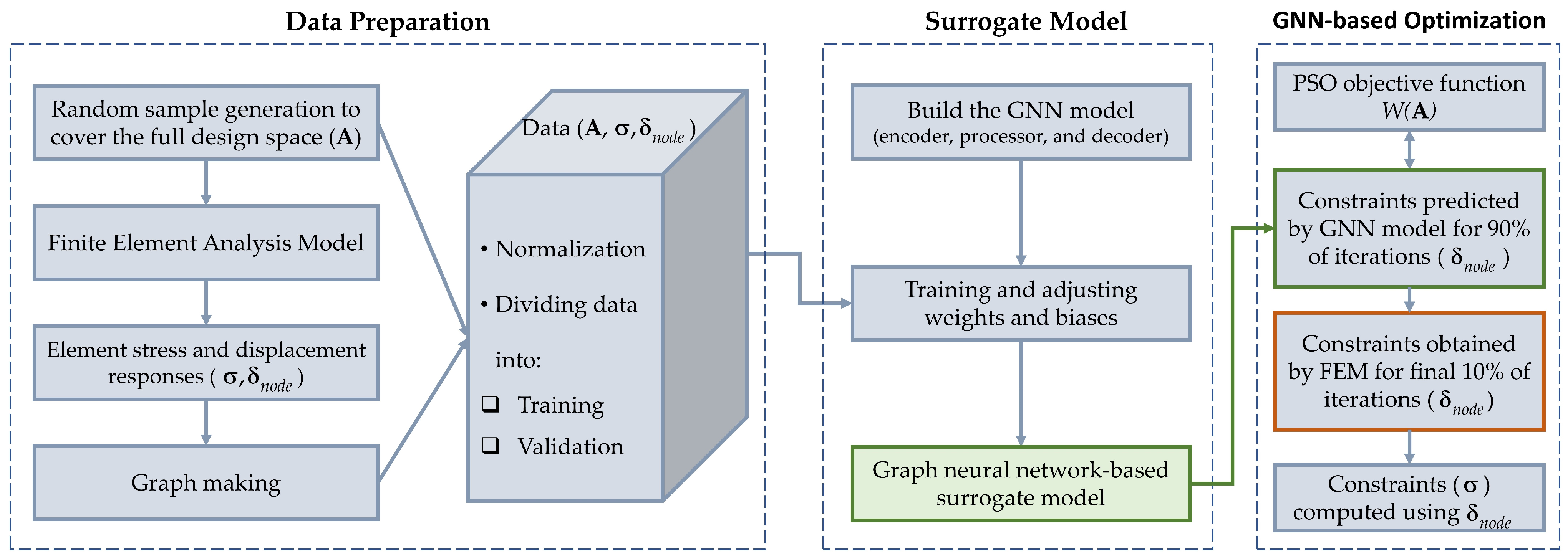
3.2. GNN-Based Optimization

In this study, a graph neural network (GNN)-based optimization technique is developed to address truss size optimization problems. In the proposed technique, a trained GNN is employed to approximate the values of constraint functions for various structural designs during most of the iterations in the PSO algorithm. Specifically, the GNN model directly approximates the nodal displacements in Equation (1), which subsequently leads to the calculation of the element stresses. By doing so, the trained GNN eliminates the need for analyzing the structural responses via FEM. This significantly improves the efficiency of the optimization process. However, given that neural network predictions may contain some degree of error, FEM analysis is used in the final iterations. In this manner, the developed technique achieves a significant enhancement in computational efficiency without compromising the reliability of the final optimal results.

A flowchart of the proposed GNN-based optimization technique is depicted in Figure 1. As shown, the technique consists of the following three main stages:

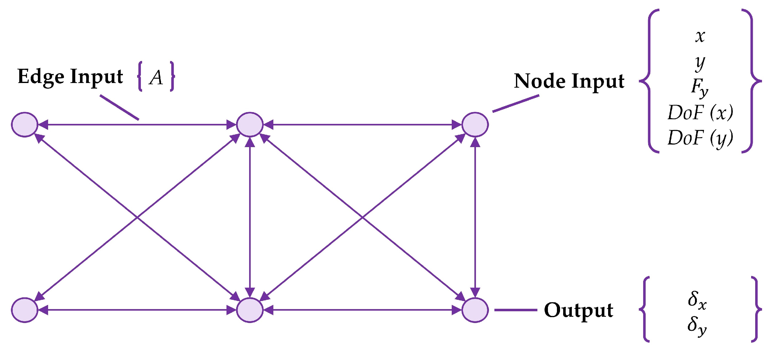
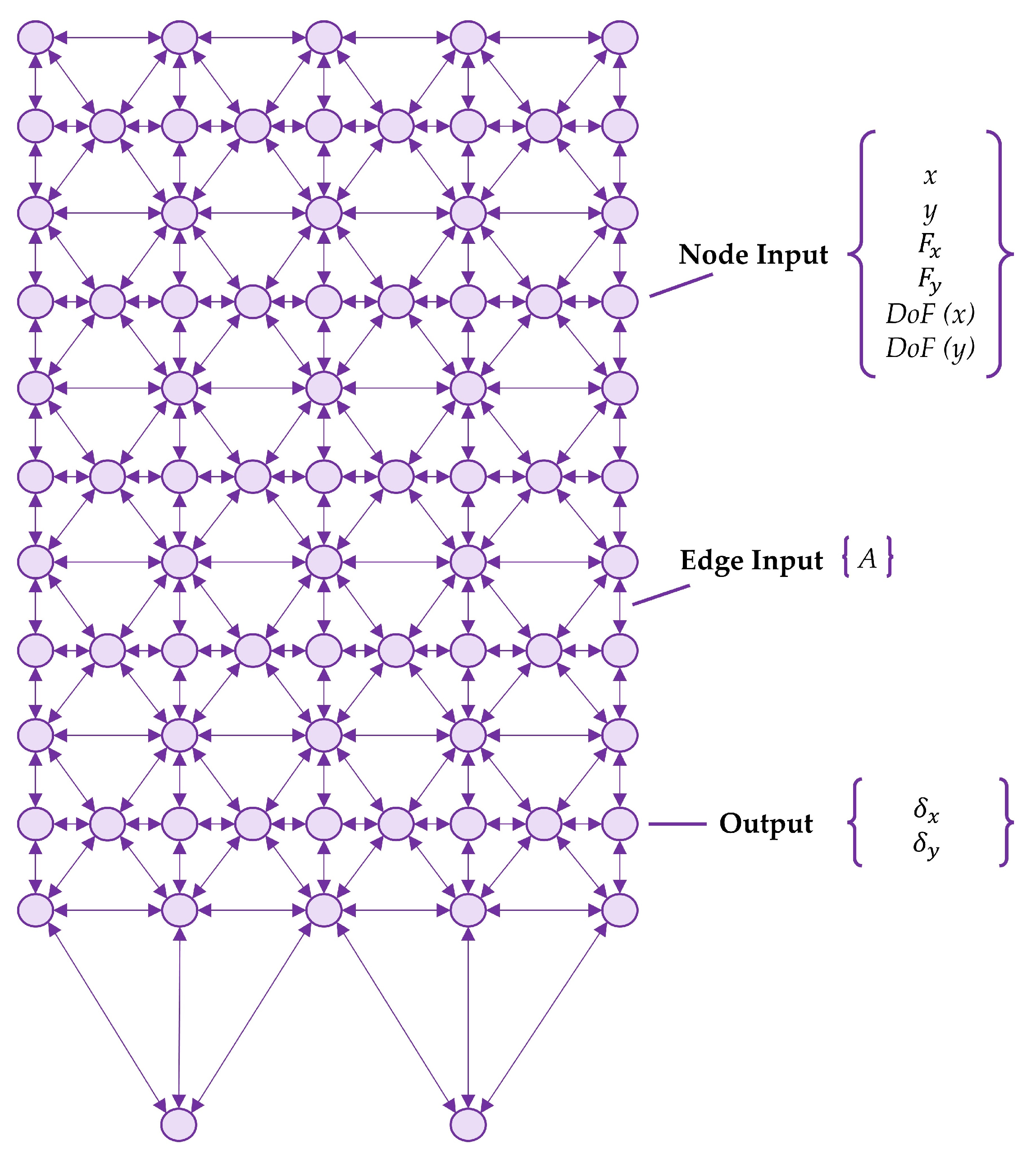
• Data Preparation. Generating a dataset of trusses with their members assigned a random sample set of cross-sectional areas, $\mathbf{A}$, which is then analyzed and transformed into graphs to be used as input to the GNN for training and validation.
• Surrogate Model. Building and training the GNN as a surrogate model for the constraints.
• Optimization. Using a PSO algorithm integrated with the trained GNN to attain the optimal cross-sectional areas of the truss members.

Details of the three stages are given below.

3.2.1. Data Preparation

For training the GNN and validating its effectiveness in approximating the nodal displacements of various designs during iterations in the PSO algorithm, a comprehensive dataset must be generated to encapsulate the structural responses of different trusses within the full design space, ${\mathbf{A}}^L\le \mathbf{A}\le {\mathbf{A}}^U$. First, a random sample set of member cross-sectional areas, $\mathbf{A}$, is generated and assigned to trusses of the same configuration, topology, and boundary conditions as the truss structure to be optimized. Second, finite element analyses of these trusses are performed to determine their nodal displacements, ${\mathbf{\delta }}_{node}$, under the same set of forces applied at the joint. The trusses are then transformed into graph representations as input to the GNN. Both the nodes and edges of the graphs are typically associated with input/output feature vectors. In this study, the cross-sectional areas of the truss members serve as the edge input feature, while the truss joint coordinates, joint external forces, and support conditions (0 for restrained directions and 1 otherwise) are the node input features. Thus, in graph representations of a three-dimensional (space) truss and two-dimensional (planar) truss, the nodal input feature vector consists of nine and six variables, respectively. The nodal output feature vector for the space and planar trusses consists, respectively, of the three and two nodal displacement components obtained from finite element analyses. Accordingly, the generated dataset used for training and validation of the GNN consists of the graphs and the input and output feature vectors of their nodes and edges.

3.2.2. Surrogate Model

The task of the surrogate model is to predict the nodal displacements of a truss using the trained GNN. To accomplish this, an Encode-Process-Decode architecture is proposed, as described in Section 3.3.2 [47]. To ensure the robustness and reliability of the model, the five-fold cross-validation technique is applied to evaluate the errors for both the training and validation datasets and to establish a suitable architecture. The network is trained using Adam optimizer [48] with the Mean Square Error (MSE) as the loss function, as given by Equation (2). In addition, the Root Mean Square Error (RMSE), as given by Equation (3), is employed as the accuracy metric for assessing the network performance.

$$\mathrm{Loss}=\mathrm{MSE}=\frac{1}{m}{\displaystyle \sum _{i=1}^m{\left(y_i-{\widehat{y}}_i\right)}^2},$$

(2)

$$\mathrm{Metric}=\mathrm{RMSE}=\sqrt{\frac{1}{m}{\displaystyle \sum _{i=1}^m{\left(y_i-{\widehat{y}}_i\right)}^2}},$$

(3)

where m is the number of training samples, and ${\widehat{y}}_i$ and $y_i$ are the predicted and target outputs, respectively.

Moreover, an initial learning rate of 0.01 is utilized, which exponentially decays at a rate of 0.5 over 500 steps. This enables the network to attain convergence and enhance the accuracy of the predictions.

The network was successfully implemented on a desktop computer equipped with a Corei7-6700HQ CPU running at 2.60 GHz and boasting 12 GB of RAM. The implementation was performed by utilizing the Spektral library, which is an open-source Python library designed for constructing graph neural networks via TensorFlow and Keras interfaces. This versatile library features an extensive array of cutting-edge techniques for deep learning on graphs, thus simplifying the GNN implementation process by offering essential building blocks [49].

3.2.3. Optimization

The proposed GNN-based optimization technique employs a GNN in conjunction with a PSO algorithm to iteratively solve a truss size optimization problem. The objective of optimization is still minimizing the total weight of the truss, while ensuring structural integrity. For prediction of the truss nodal displacements, the trained GNN is used as a surrogate model for 90% of the iterations, with the remaining 10% utilizing FEM analysis to determine more accurate nodal displacements. Subsequently, the internal stresses of the truss elements are calculated based on the nodal displacements and axial deformations of the elements. Notably, to improve diversity of the PSO optimization process, which is discussed in Section 3.4, the population size is increased when the GNN prediction model is substituted with FEM analysis. This allows new particles to join the optimization process and helps ensure more population diversity. The final obtained set of cross-sections are, therefore, highly trustworthy, as they have been rigorously verified using FEM analyses during the final iterations. By integrating the power of the GNN and PSO algorithm, this optimization technique provides an efficient solution for truss size optimization, with potential applications in a wide range of structural designs, particularly for large structures.

3.3. Graphs and Graph Neural Networks

Graph neural networks represent a specialized category of artificial neural networks that are specifically engineered to leverage the benefits of data structured as a graph. This is applicable in two common scenarios: in some applications, the dataset is inherently organized as graphs, such as the data associated with molecules and physical systems. However, in other cases, graphs can be implicit and require structuring, such as word graphs for text interpretation [50]. Truss structures can be represented as graphs by considering the joints as vertices and the members as edges. Once the graph data are structured, the existing relationships within the graphs can be learned by establishing an optimal graph neural network architecture.

Graphs serve as mathematical structures employed for modeling a group of objects along with their relationships. A graph is made up of a collection of vertices or nodes connected by edges or links. In this context, a graph can be denoted as $G=(\mathbf{X},\hspace{0.17em}\mathbf{E})$, where $\mathbf{X}$ and $\mathbf{E}$ are node and edge features, respectively; $‖\mathbf{X}‖=N_n$ is the number of nodes; and $‖\mathbf{E}‖=N_e$ is the number of edges.

Graphs can be classified based on several parameters, some of which are [50]:

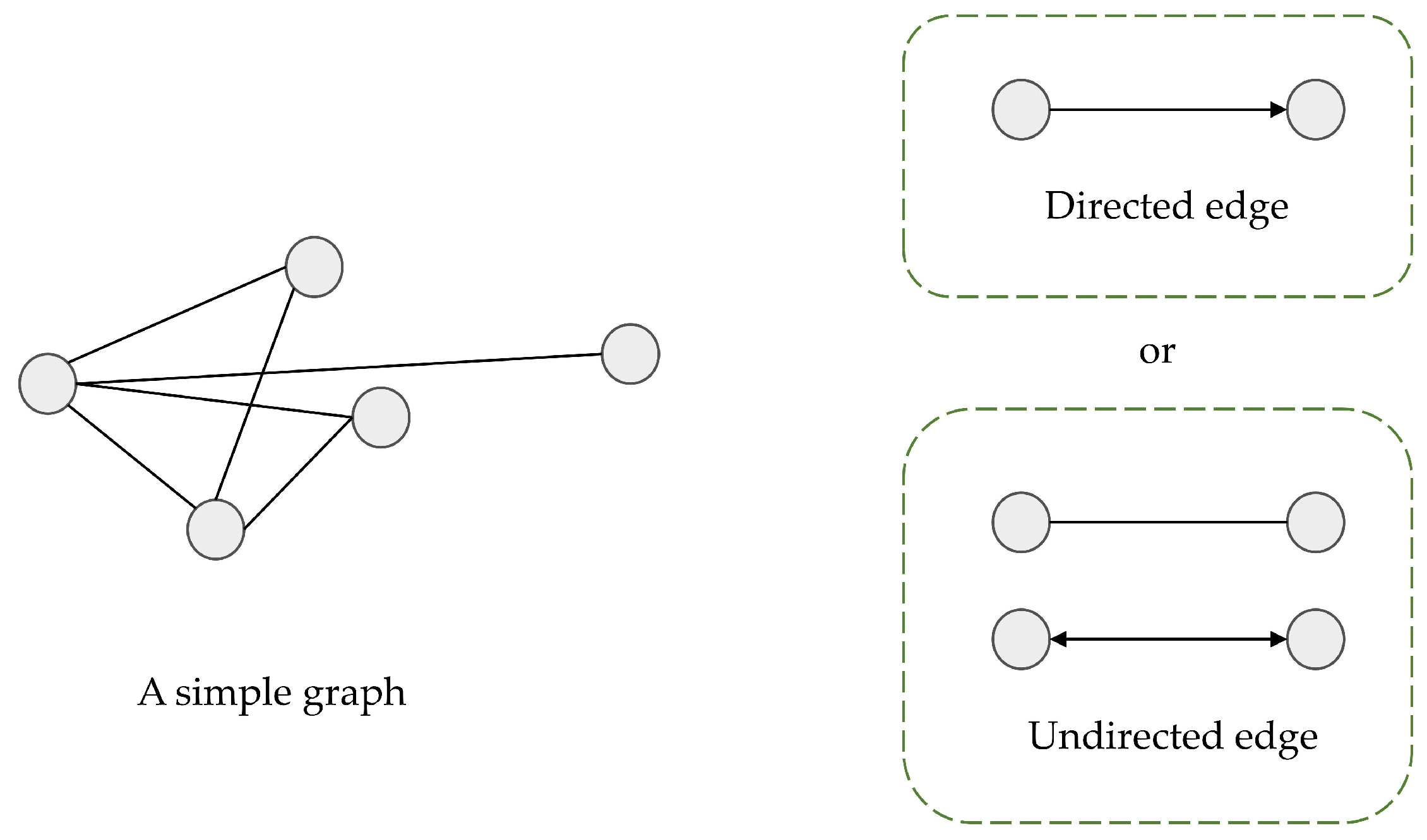
• Directed or undirected graphs. In directed graphs, directional dependencies exist between nodes, and edges only go from one node to another. In contrast, in undirected graphs, edges are considered undirected or bidirectional. Figure 2 illustrates examples of the two edge types.
• Homogeneous or heterogeneous graphs. Vertices and edges are of the same types in homogenous graphs, whereas they have different types in heterogenous graphs. The latter can be important information in further usage of the graph datasets.
• Static or dynamic graphs. The graph is regarded as dynamic when input features or graph configuration changes over time.

The information storage capabilities of vertices and edges in a graph are sufficient for prediction tasks. Such tasks can fall into one of three categories: the node-level, edge-level, and graph-level prediction [50]:

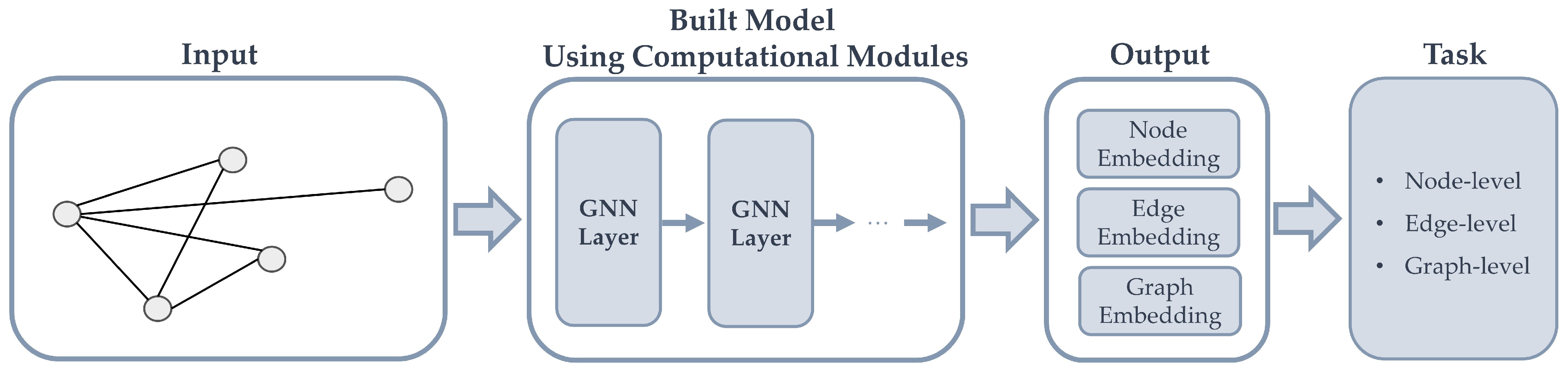
• Node-level prediction tasks revolve around node attributes and their roles within a graph. Node classification, node regression, and node clustering are examples of node-level prediction tasks. In node classification, nodes are categorized in a variety of predetermined classes. Node regression aims to predict continuous variables for each node. On the other hand, the goal of node clustering is to make groups of unlabeled nodes with similar attributes.
• Edge-level prediction tasks are edge classification, regression, and link prediction. Here, edge classification pertains to classifying edge types, while edge regression deals with continuous variables associated with edges. Link prediction involves determining the presence or absence of an edge between two given nodes.
• Graph-level prediction tasks seek to predict the properties of an entire graph, including graph classification, graph regression, and graph matching. While the notion of graph classification and regression mirrors that of other types of prediction tasks, the classes and continuous variables are now for the entire graph. Graph matching, meanwhile, aims to investigate the similarity of graphs.

3.3.1. Computational Modules

A typical GNN model usually comprises a multitude of computational modules. Some widely used modules are [50]:

• Propagation Modules. Propagation modules are used to propagate information through nodes so that an aggregated representation of the graph’s configuration and features are created. Notably, convolution operators serve as propagation modules, as they allow for aggregation of information from the neighboring nodes.
• Sampling Modules. For large-scale graphs, i.e., graphs that cannot be stored and processed by the device, sampling modules work in conjunction with propagation modules to propagate information effectively across the graph.
• Pooling Modules. Pooling modules play a crucial role in extracting information from nodes to construct high-level representations of subgraphs or graphs.

Figure 3 illustrates a typical architecture of a GNN model tailored to analyze graph-structured data. The model receives input in the form of graphs and generates embeddings for the nodes, edges, and the entire graph as its output, drawing upon the particular prediction task at hand. These embeddings comprise vector representations that capture crucial information concerning the graph configuration, as well as the relationships among the nodes. The GNN model incorporates a range of modules, including propagation, sampling, and pooling, which work together to facilitate the transmission of information throughout the various layers.

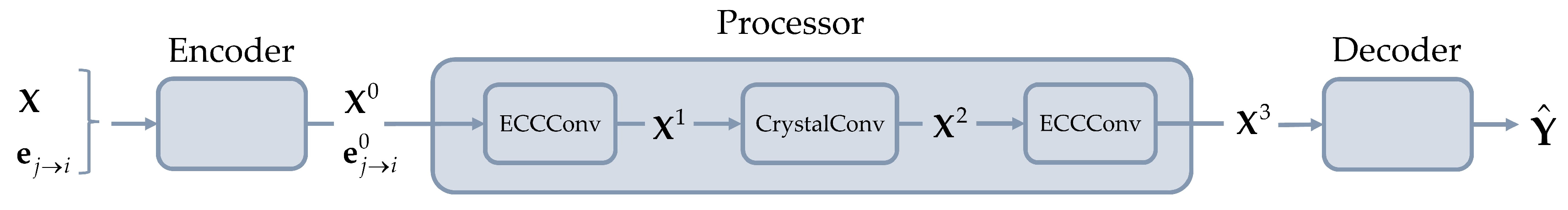
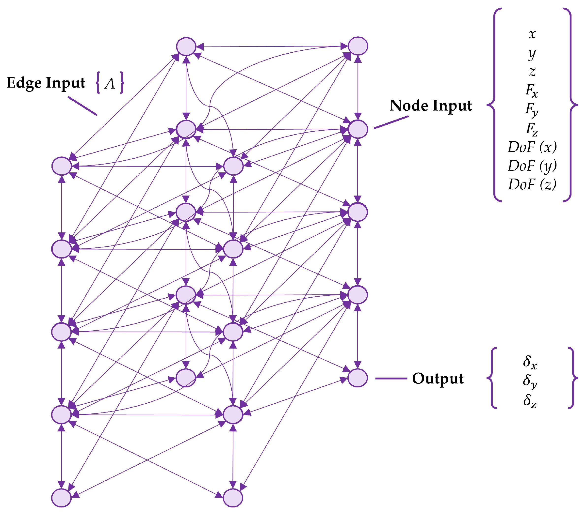
3.3.2. Encode-Process-Decode Architecture

The objective is to utilize a GNN-based surrogate model that has been trained to predict the nodal displacements of a truss within a node-level prediction task. This is achieved using an Encode-Process-Decode architecture (see Figure 4) which comprises distinct components that work in tandem, with the inputs being trusses structured as undirected, homogeneous, and static graphs. The encoder constructs latent node and edge features, ${\mathbf{X}}^0$ and ${\mathbf{e}}_{j\to i}^0$, based on the inputs, $\mathbf{X}$ and ${\mathbf{e}}_{j\to i}^{}$. The processor then performs three convolutional layers across the latent node and edge features, ${\mathbf{X}}^1,{\mathbf{X}}^2$, and ${\mathbf{X}}^3$. Ultimately, the decoder extracts structural responses, $\widehat{\mathbf{Y}}$, from the final latent node features, ${\mathbf{X}}^3$. This section provides an overview of each component of the network architecture.

3.3.2.1. Encoder

Each node and edge in the graphs contain a feature vector that represents its characteristics. Two encoders are utilized to set the initial state of the node and edge representations by separately transforming each of the feature vectors into embeddings with different sizes of vectors. The encoders take the original feature vectors of the nodes and edges as inputs and apply non-linear transformations to obtain the embedded representations. A simple Multilayer Perceptron (MLP) with two 8-unit layers is employed to encode the features of each node, resulting in a latent vector of size 16. Likewise, edge features are also encoded using an MLP with an identical architecture, yielding a latent vector of size 16 for each edge. The rectified linear unit (ReLu) is utilized as the activation function of the encoders, which is known for its ability to reduce sparsity and facilitate the learning process. Therefore, the embeddings generated by the encoders capture the characteristics and information of each node and edge in an increased dimensional space, which are used for further processing to learn meaningful node representations.

3.3.2.2. Processor

The embeddings obtained from the encoders are used for iterative message-passing and node updates. In each layer of the processor, the embeddings of a node are aggregated with the embeddings of its neighbors and connecting edges, collecting knowledge from the node’s neighborhood for updating its own embeddings. The processor comprises three convolutional layers, with a central layer named CrystalConv nestled between the two additional layers known as ECCConv. This selection of layer types was made due to their remarkable ability to incorporate edge features—a critical component in the training process. Both layer types are described below:

• ECCConv Layer is an Edge-Conditioned Convolution (ECC) layer that not only captures the features of individual nodes, but also ties the weights, ${\mathbf{W}}^l$, to the edge features in each layer $l$. The output of ECCConv layers in this study takes the form of a vector with 64 distinct components. The ECC convolution layer is mathematically formulated as a function of both the node and edge features in the following manner [51]:

  $${\mathbf{X}}_i^l={\mathbf{X}}_i^{l-1}\hspace{0.17em}{\mathbf{W}}_{root}+{\displaystyle \sum _{j\in N(i)}{\mathbf{X}}_j^{l-1}\hspace{0.17em}\mathrm{M}\mathrm{L}\mathrm{P}}\left({\mathbf{e}}_{j\to i}^l\right)+{\mathbf{b}}^l,$$

  (4)

  where ${\mathbf{X}}^l$ and ${\mathbf{e}}_{j\to i}^l$ are the node and edge features of layer $l$, respectively. ${\mathbf{W}}_{root}$ is the weight for the node features of the previous layer. A neighborhood $N(i)=\{j;(j,i)\in \mathbf{E}\}$ of vertex $i$ includes all adjacent vertices $j$. MLP is a multilayer perceptron that outputs an edge-specific weight, ${\mathbf{W}}^l$, as a function of the edge features. ${\mathbf{b}}^l$ is the bias vector as a model parameter being updated and optimized during the training process.
• CrystalConv is a Crystal Convolution layer introduced by Xie and Grossman [52]. This layer computes:

  $${\mathbf{X}}^l(i)={\mathbf{X}}^{l-1}(i)+{\displaystyle \sum _{j\in N(i)}\sigma }\left({\mathbf{Z}}_{ij}^{l-1}\hspace{0.17em}{\mathbf{W}}_f^l+{\mathbf{b}}_f^{l-1}\right)\odot g\left({\mathbf{Z}}_{ij}^{l-1}\hspace{0.17em}{\mathbf{W}}_s^l+{\mathbf{b}}_s^{l-1}\right),$$

  (5)

  where ${\mathbf{Z}}_{ij}^{l-1}={\mathbf{X}}_i^{l-1}\oplus {\mathbf{X}}_j^{l-1}\oplus \hspace{0.33em}{\mathbf{e}}_{j\to i}^{l-1}$ concatenates neighbor vectors with the features of the connecting edge. Meanwhile, $\odot$ indicates an element-wise multiplication; $\mathrm{\sigma }(\cdot )$ denotes a sigmoid function; and $g(\cdot )$ is an activation function defined by the user. In this work, summation pooling and ReLU are used as the pooling and activation functions, respectively.

3.3.2.3. Decoder

The decoder follows the processor by separately taking the final node representations obtained after the message-passing and node updates to provide a fixed-length output vector for each node. An MLP with two 8-unit layers is utilized to decode the features of each node to a latent vector that aligns with the required size of the nodal outputs. Therefore, the defined decoder can produce final outputs that consist of two components for 2D trusses and three components for 3D trusses.

3.4. PSO Implementation

Various metaheuristic algorithms have been employed to tackle truss size optimization problems. In 1995, Kennedy et al. [53] developed a new evolutionary algorithm called particle swarm optimizer (PSO). It is a mathematical method imitating the behavior of a swarm of birds flocking or a school of fish searching for food. This algorithm has fewer parameters and, in turn, is simpler to implement than other available methods, such as genetic algorithms. Also, PSO exhibits a faster convergence rate than other evolutionary algorithms for solving several optimization problems [54]. This algorithm involves a swarm of individual particles, each of which represents a point within the M-dimensional search space, where M is the number of parameters to be optimized. A particle possesses a fitness value and a velocity, which are continuously updated to steer the particle towards the best experience of the swarm. The velocity $V_i^m$ and position $K_i^m$ of the mth dimension of the ith particle are updated as follows [53,55]:

$$V_i^m\leftarrow w\times V_i^m+c_1\times rand{1}_i^m\times \left(pbes{t}_i^m-K_i^m\right)+c_2\times rand{2}_i^m\times \left(gbes{t}^m-K_i^m\right),$$

(6)

$$K_i^m\leftarrow K_i^m+V_i^m,$$

(7)

where ${\mathbf{K}}_i=\left\{K_i^1,K_i^2,K_i^3,\cdots ,K_i^M\right\}$ and ${\mathbf{V}}_i=\left\{V_i^1,V_i^2,V_i^3,\cdots ,V_i^M\right\}$ are vectors representing, respectively, the position and velocity of the ith particle; $w$ is the inertia weight balancing the global and local search abilities. A large inertia weight facilitates global search, while a small inertial weight is more suitable for local search. In this study, a method of linearly decreasing the inertia weight over the optimization process [56] is employed. By doing so, the inertia weight is set to 0.9 at the initial point $\left(w_0=0.9\right)$. During the optimization, the weight decreases linearly to reach 0.4 at the end of the process $\left(w_{end}=0.4\right)$.

The vector $\mathbf{p}\mathbf{b}\mathbf{e}\mathbf{s}{\mathbf{t}}_i=\left\{pbes{t}_i^1,pbes{t}_i^2,pbes{t}_i^3,\cdots ,pbes{t}_i^M\right\}$ is the best previous position that resulted in the best fitness (objective) value for the ith particle, and the vector $\mathbf{g}\mathbf{b}\mathbf{e}\mathbf{s}{\mathbf{t}}_i=\left\{gbes{t}_i^1,gbes{t}_i^2,gbes{t}_i^3,\cdots ,gbes{t}_i^M\right\}$ is the best position yielded by the entire population. $c_1$ and $c_2$ are the acceleration constants reflecting the weighting of each stochastic acceleration terms $\left(c_1=c_2=2\right)$. They determine the relative amount of particle movements towards $\mathbf{p}\mathbf{b}\mathbf{e}\mathbf{s}\mathbf{t}$ and $\mathbf{g}\mathbf{b}\mathbf{e}\mathbf{s}\mathbf{t}$ positions. Also, $rand{1}_i^m$ and $rand{2}_i^m$ are two random numbers sampled uniformly in the range [0, 1]. There are minimum and maximum possible velocity vectors $\left[{\mathbf{V}}^{min},{\mathbf{V}}^{max}\right]$ as boundaries defined by the user to limit the velocity of the particle. Considering that the search range for a problem is $\left[{\mathbf{K}}^{min},{\mathbf{K}}^{max}\right]$, the minimum and maximum velocity vectors are defined as follows:

$${\mathbf{V}}^{min}=-0.2\left({\mathbf{K}}^{max}-{\mathbf{K}}^{min}\right),$$

(8)

$${\mathbf{V}}^{max}=+0.2\left({\mathbf{K}}^{max}-{\mathbf{K}}^{min}\right).$$

(9)

Algorithm 1 outlines the step-by-step procedure of the PSO algorithm, which is programmed based on Reference [55]. Subsequently, the program is enhanced to incorporate the fitness (objective) function and manage the constraints, specifically to solve truss size optimization problems.

Algorithm 1 Particle Swarm Optimization algorithm
INPUT:	Initialize the population of particles:
	Set the maximum number of iterations.
	Set the number of particles in the swarm.
	Randomly initialize the position and velocity of each particle. Determine the fitness value of each particle.
	Set the personal best position (pbest) of each particle as its initial position.
	Determine the global best position (gbest) of the population.
OUTPUT:	gbest and its fitness value found in the final iteration.
1.	For each iteration until the maximum number of iterations is reached:
2.	Update the velocity and position of each particle using the formulas:
3.	$V_i^m\leftarrow w\times V_i^m+c_1\times rand{1}_i^m\times \left(pbes{t}_i^m-K_i^m\right)+c_2\times rand{2}_i^m\times \left(gbes{t}^m-K_i^m\right)$
4.	$K_i^m\leftarrow K_i^m+V_i^m$
5.	Evaluate the fitness of the new position of each particle.
6.	Update the pbest and gbest:
7.	If the fitness of the new position is better than its pbest fitness:
	Update pbest.
	Check if the fitness of pbest is better than the gbest fitness:
8.	Update gbest.

3.4.1. Handling of Size Optimization Constraints

Structural design must satisfy several requirements, including but not limited to resistance and serviceability. As such, truss size optimization is inevitably subject to several design constraints; see Equation (1). For handling the constraints, the penalty function, $P(\cdot )$, is employed, which is formulated as shown in the following [57,58]:

$$P(\mathbf{A})=W(\mathbf{A})\times {\phi }_p\times B,$$

(10)

$${\phi }_p={(1+C)}^{\epsilon },$$

(11)

where $B$ and $\epsilon$ describe the penalty coefficient and penalty exponent, which are taken in this study as 1 and 2, respectively. As before, $\mathbf{A}=\left\{A_1,A_2,A_3,\cdots ,A_{ne}\right\}$ are the size variables, and $W$ is the resultant total weight of the structure. Additionally, the violation measurement $C$ is determined by the following equation:

$$C={\displaystyle \sum _{j=1}^{ne}{C}_{\sigma }^j}+{\displaystyle \sum _{i=1}^{nj}{C}_{\delta }^i},$$

(12)

$$\begin{array}{l}{C}_{\sigma }^j=\left|\frac{\left|{\sigma }_j\right|-{\sigma }_a}{{\sigma }_a}\right|\hspace{1em}\hspace{1em}\hspace{1em}\hspace{0.33em}\mathrm{if}\hspace{0.33em}\hspace{0.33em}\left|{\sigma }_j\right|>{\sigma }_a\\ \\ C_{\sigma }^j=0\hspace{1em}\hspace{1em}\hspace{1em}\hspace{0.17em}\hspace{1em}\hspace{1em} \mathrm{if}\hspace{0.33em}\hspace{0.33em}\left|{\sigma }_j\right|<{\sigma }_a\end{array},$$

(13)

$$\begin{array}{l}{C}_{\delta }^i=\left|\frac{\left|{\delta }_i\right|-{\delta }_a}{{\delta }_a}\right|\hspace{1em}\hspace{1em}\hspace{1em} \mathrm{if}\hspace{0.33em}\hspace{0.33em}\left|{\delta }_i\right|>{\delta }_a\\ \\ C_{\delta }^i=0\hspace{1em}\hspace{1em}\hspace{1em}\hspace{1em}\hspace{1em} \mathrm{if}\hspace{0.33em}\hspace{0.33em}\left|{\delta }_i\right|<{\delta }_a\end{array},$$

(14)

where $C_{\sigma }^{\hspace{0.17em}j}$ and $C_{\mathbf{\delta }}^{\hspace{0.17em}i}$ are associated with the stress and displacement constraints, thereby expressing the constraints in normalized forms. The parameters ne and nj correspond to the number of truss elements and truss joints, respectively. Other relevant parameters have been defined in Equation (1).

4. Results and Discussion

The developed GNN-based optimization technique is used to solve three truss size optimization problems: (1) a 10-bar planar truss, (2) a 72-bar space truss, and (3) a 200-bar planar truss. To verify the validity and effectiveness of the proposed technique, a FEM-based PSO optimization technique is also developed in Python. The FEM-based optimization adopts a simple finite element approach to analyze truss structures and determine the corresponding nodal displacements and element stresses. The results of the FEM-based optimization are used as a benchmark for validating and verifying the optimal solutions obtained from the GNN-based model.

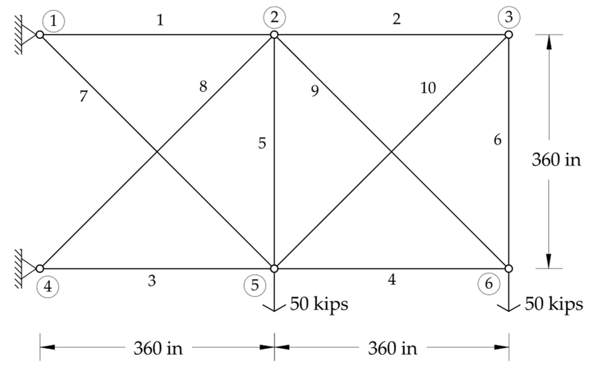
4.1. Ten-Bar Planar Truss

The considered 10-bar planar truss problem is commonly used as a starting point when assessing new optimization methods. The truss illustrated in Figure 5 consists of six joints connected by ten elements. The process of optimizing the size of this structure necessitates the use of 10 distinct design variables, namely, the cross-sectional areas of the 10 truss elements. The cross-sectional areas are selected from the range of [1, 15] in².

Table 1. Design parameters of the 10-bar planar truss.

Parameter	Value
Modulus of elasticity	10,000 ksi
Material density	0.1 lb/in3
Allowable stresses	±25 ksi
Allowable nodal displacement	2 in

presents a summary of the design parameters used for this problem.

4.1.1. Data Preparation

The initial stage involved generating truss structural design samples with element cross-sectional areas within a defined space of $\mathbf{A}\hspace{0.33em}\in \hspace{0.33em}[1,\hspace{0.17em}15]$ in². Specifically, 1000 truss structural design samples were generated, whereby for each truss sample, 10 design variables were randomly assigned values within the specified range. The trusses were then analyzed using a finite element model, and the nodal displacements determined from the analysis were stored along with other information pertaining to the truss configuration. These data were subsequently utilized to create graphs representing the truss structures. Since the 10-bar planar truss is two-dimensional, and the applied loads are vertical, five node features are sufficient to effectively represent the truss. As shown in Figure 6, these features include the truss joint coordinates $\left(x,\hspace{0.17em}y\right)$, the vertical load $\left(F_y\right)$ applied at the joints, and the two binary features (0 or 1) indicating the degrees of freedom associated with the joint translations. Additionally, each edge has a single feature that pertains to the corresponding truss element’s cross-sectional area, A, while each node contains two output features that correspond to the nodal displacements $\left({\delta }_x,\hspace{0.17em}{\delta }_y\right)$ obtained via FEM.

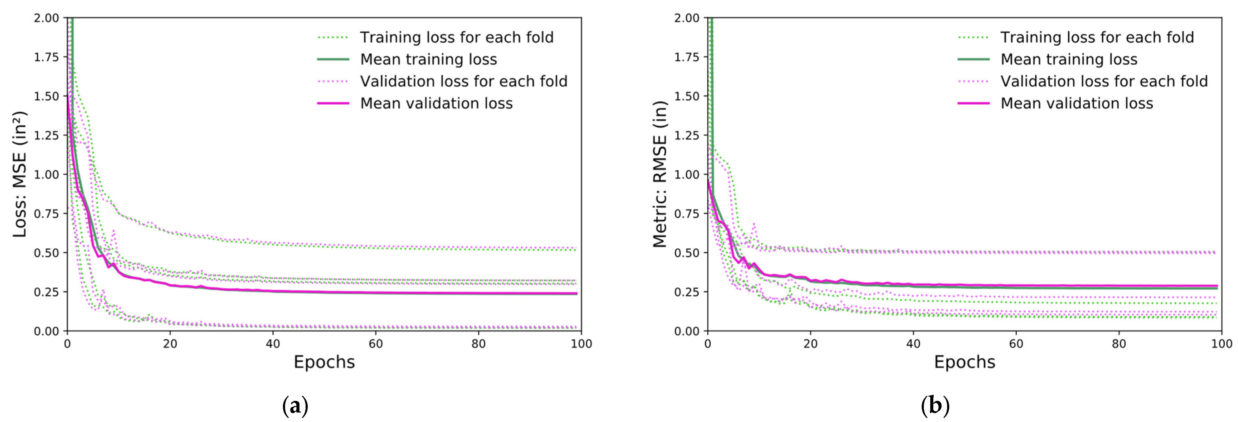
4.1.2. GNN Model Training

The performance of the graph neural network was assessed using the five-fold cross-validation method. Figure 7 presents the learning curves of the training and validation datasets for the loss and metric functions. As can be seen, the curves for both datasets exhibit a gradual flattening, which provides evidence that the models have been adequately trained. Meanwhile, the risk of overfitting is deemed to be negligible, given the minimal difference between the training and validation loss learning curves. To supplement this, the mean values for both MSE and RMSE across all five training and validation sets are shown in

Table 2. Mean results of five-fold cross-validation for 10-bar truss.

	Training	Validation
MSE (in2)	0.236	0.240
RMSE (in)	0.271	0.288

.

To enhance the nodal displacements prediction accuracy, the surrogate model was trained utilizing the entire dataset comprising all 1000 truss samples (Figure 8). The figure shows an accurate performance of the model measured by the mean square error, MSE = 0.022 at the end of training.

4.1.3. GNN-Based Optimization

The proposed GNN-based optimization was validated by a simple FEM-based optimization, in which the PSO algorithm evaluates each particle via a finite element analysis. It should be noted that the population of the GNN-based optimization was set to 75 and increased to 150 in the final 10% of iterations, compared to the fixed population of 75 for the FEM-based optimization over the course of all 100 iterations. The optimum outcomes for the 100 independent runs of each optimization technique are presented in

Table 3. Optimal design for the 10-bar planar truss.

Variables		Cross-Sectional Areas (in2)
Element Group	Members	FEM-Based Optimization (Benchmark)	GNN-Based Optimization
1	1	15.000	15.000
2	2	1.000	1.000
3	3	12.268	12.012
4	4	7.644	7.660
5	5	1.000	1.000
6	6	1.000	1.000
7	7	4.684	4.943
8	8	11.202	11.088
9	9	10.913	10.966
10	10	1.000	1.000
${\left|{\delta }_{node}\right|}^{\max }$ (in)		2.00	2.00
${\left|\sigma \right|}^{\max }$ (ksi)		12.49	12.04
Weight (lb)		2780.09	2781.56
Nanalyses		7500	2500

, with the GNN-based optimization reaching the optimal weight with a negligible 0.05% deviation from the results of the FEM-based optimization. As for computational efficiency, the FEM-based optimization required an average of 9.3 s to attain an optimal solution with 7500 analyses. In contrast, the GNN-based optimization took 221.7 s, including 3.2 s for the data preparation and 218.5 s for the optimization process. A total of 2500 FEM analyses were performed by the GNN-based optimization, of which 1000 were to generate training samples and 1500 analyses were in the last ten iterations for 150 particles in each iteration. Despite using fewer FEM analyses than the FEM-based optimization, the GNN-based optimization required more time to achieve the optimal solution. This is because the 10-bar planar truss is a simple problem that lends itself to simple analysis, and therefore, the needed time to analyze the simple truss is less than that required for GNN predictions.

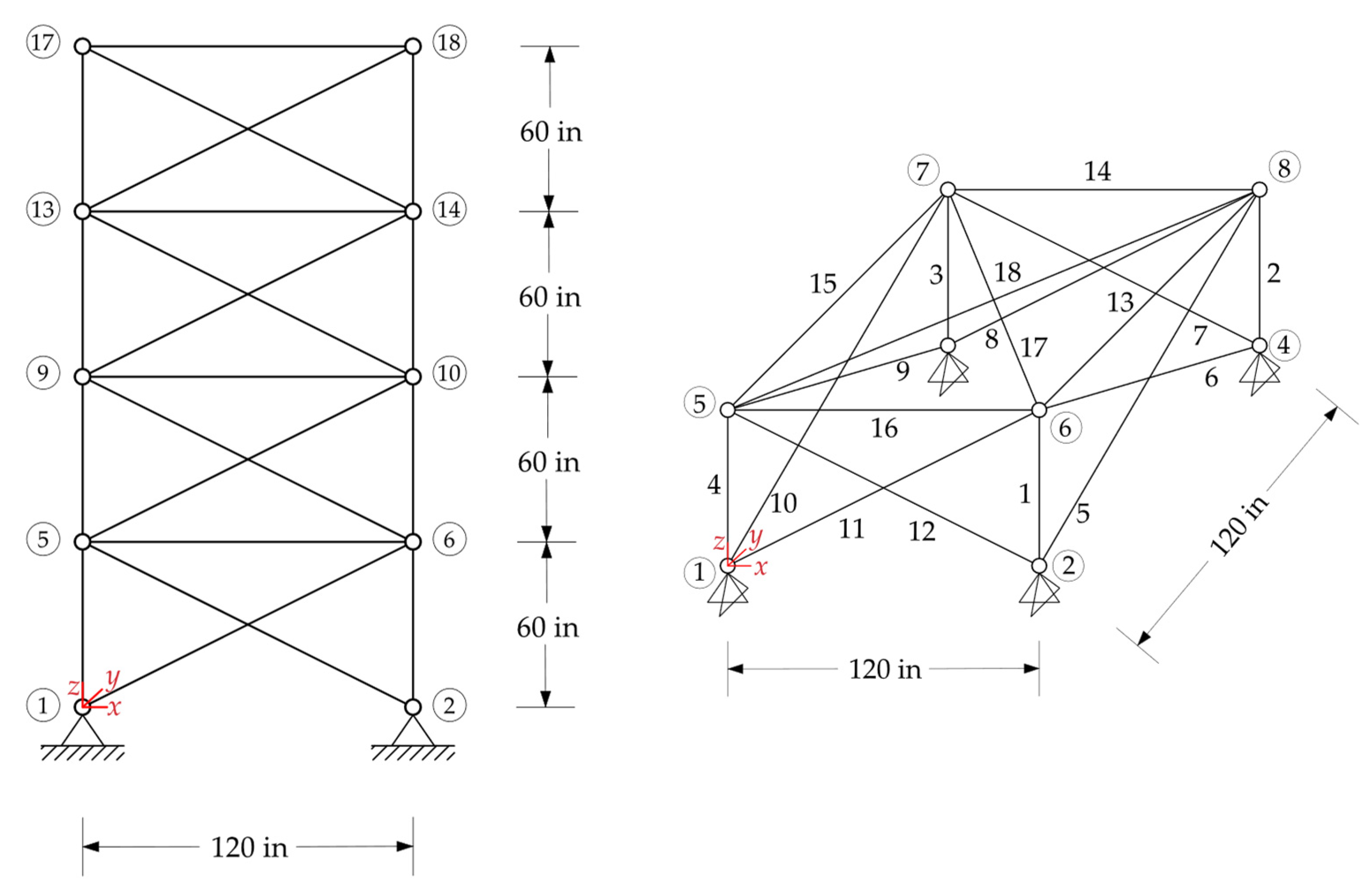
4.2. Seventy-Two-Bar Space Truss

Figure 9 shows a 72-bar multi-story space truss consisting of 20 joints connected by 72 elements. To simplify the design process and make use of the structural symmetry, the 72 elements were classified into 16 groups. Thus, the number of design variables was reduced to 16, which represent the cross-sections of truss elements in each group. These cross-sections were chosen within the range of 0.1 in² to 3 in². The design parameters used to solve the size optimization problem are summarized in

Table 4. Design parameters of the 72-bar space truss.

Parameter	Value
Modulus of elasticity	10,000 ksi
Material density	0.1 lb/in3
Allowable stresses	±25 ksi
Allowable nodal displacement	0.25 in

. The applied loading case is also presented in

Table 5. Applied loads on the 72-bar space truss.

Joint	Px (kips)	Py (kips)	Pz (kips)
18	5	5	−5
19	5	5	−5

.

4.2.1. Data Preparation

A thousand truss structural design samples were generated in a defined space of $\mathbf{A}\hspace{0.33em}\in \hspace{0.33em}[0.1,3]\hspace{0.33em}\hspace{0.17em}{\mathrm{in}}^2$, with the 16 design variables being assigned random values within the specified range for each sample. Each generated structure was analyzed using a finite element model. The results of the structural analyses were subsequently used to create a graph-structured dataset that contained nine distinct features for each node. As presented in Figure 10, the features of each node are the truss joint coordinates $\left(x,y,z\right)$, the applied joint loads $\left(F_x,\hspace{0.17em}{F}_y,F_z\right)$, and the three binary features (0 or 1) representing the degrees of freedom associated with the translations of the joint. Once again, each edge has a single feature that pertains to the corresponding truss element’s cross-sectional area, A. Also, each node has three output features, namely, the nodal displacements $\left({\delta }_x,\hspace{0.17em}{\delta }_y,\hspace{0.17em}{\delta }_z\right)$ obtained from the FEM analysis.

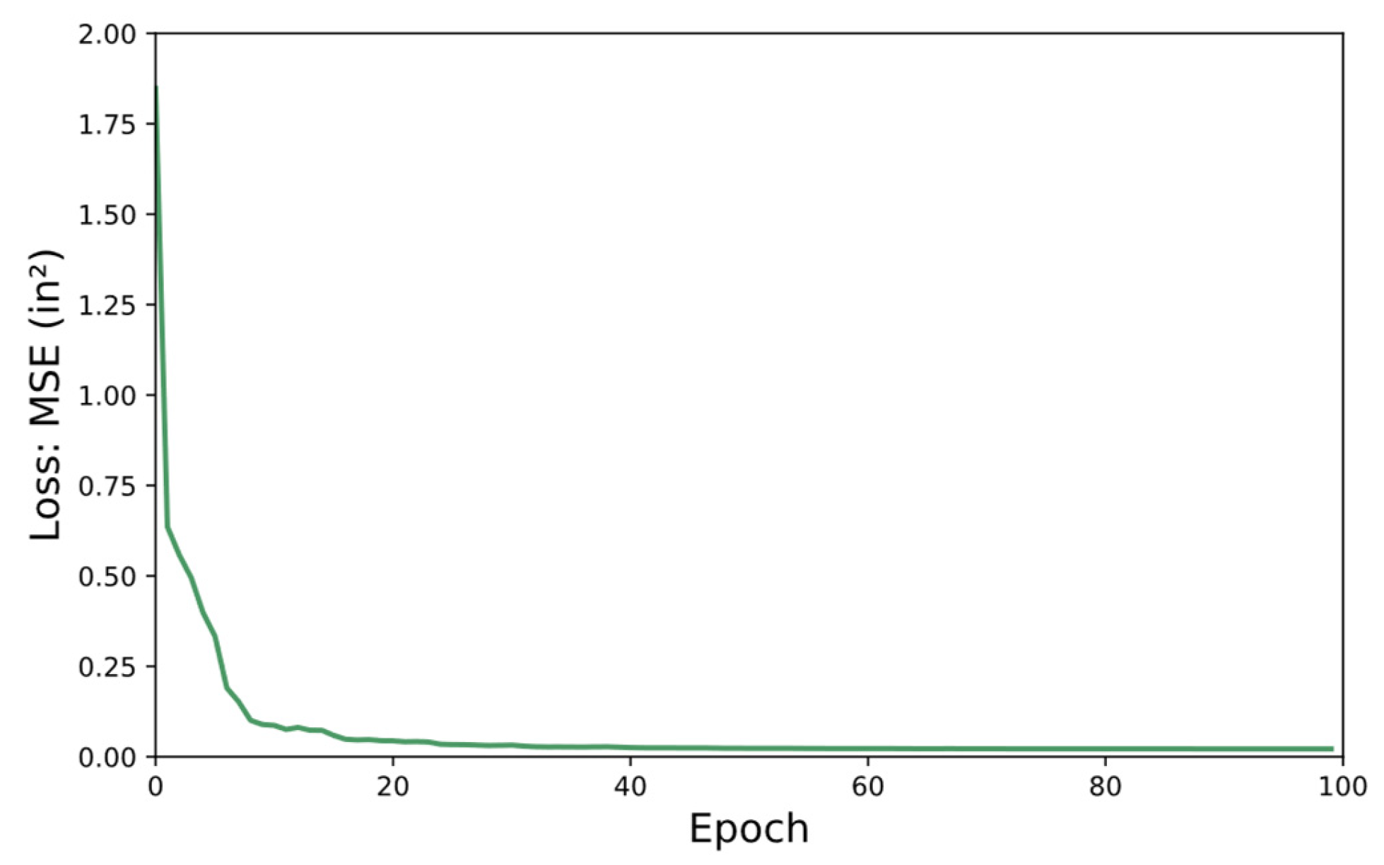
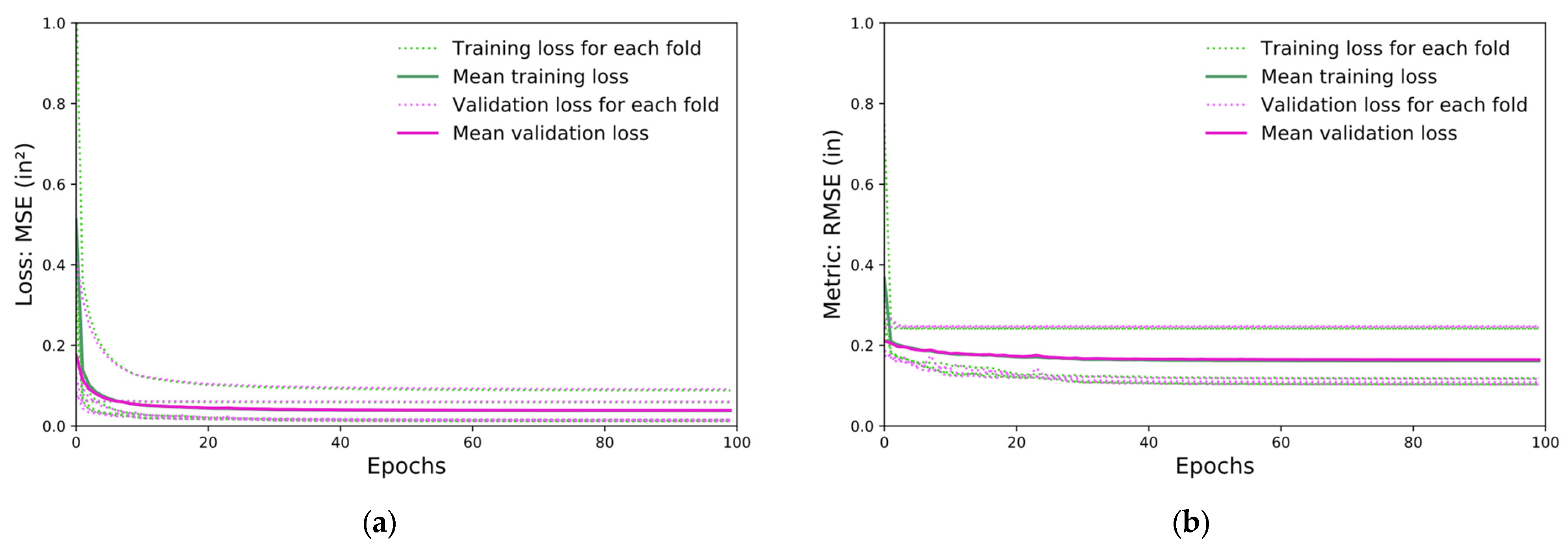
4.2.2. GNN Model Training

The graph neural network was evaluated using the five-fold cross-validation technique, as depicted in Figure 11. The calculated mean values of MSE and RMSE for the training and validation datasets across all the five folds are shown in

Table 6. Mean results of five-fold cross-validation for 72-bar truss.

	Training	Validation
MSE (in2)	0.038	0.039
RMSE (in)	0.162	0.164

. The surrogate model used in the GNN-based optimization was trained using all 1000 truss samples, as shown in Figure 12, and the resulting final mean square error was MSE = 0.019 in².

4.2.3. GNN-Based Optimization

The population of the GNN-based optimization began at 75 and increased to 150 in the final 10% of iterations, whereas the FEM-based optimization population was 75 throughout all 100 iterations.

Table 7. Optimal design for the 72-bar space truss.

Variables		Cross-Sectional Areas (in2)
Element Group	Members	FEM-Based Optimization (Benchmark)	GNN-Based Optimization
1	1–4	3.000	3.000
2	5–12	2.210	2.186
3	13–16	0.109	0.100
4	17, 18	0.100	0.100
5	19–22	3.000	3.000
6	23–30	2.207	2.184
7	31–34	0.100	0.100
8	35, 36	0.100	0.100
9	37–40	3.000	3.000
10	41–48	2.148	2.036
11	49–52	0.100	0.100
12	53, 54	0.100	0.100
13	55–58	1.627	1.851
14	59–66	2.113	2.200
15	67–70	0.719	0.817
16	71, 72	0.250	0.264
${\left|{\delta }_{node}\right|}^{\max }$(in)		0.25	0.25
${\left|\sigma \right|}^{\max }$(ksi)		7.91	7.90
Weight (lb)		1254.68	1256.94
Nanalyses		7500	2500

presents the best results for the 100 independent runs of each optimization technique. Remarkably, the achieved optimal structural weight exhibits a high accuracy with a negligible difference of less than 0.2% from the outcomes of the FEM-based optimization. In terms of computational time, the FEM-based optimization required an average of 68.7 s with 7500 analyses, while the GNN-based optimization needed 242.6 s for prediction, comprising 13.1 s for the data preparation and 229.5 s for the optimization stage. As before, the GNN-based optimization required a total of 2500 FEM analyses, including 1000 analyses to generate training samples and 1500 analyses in the last 10 iterations for 150 particles in each iteration.

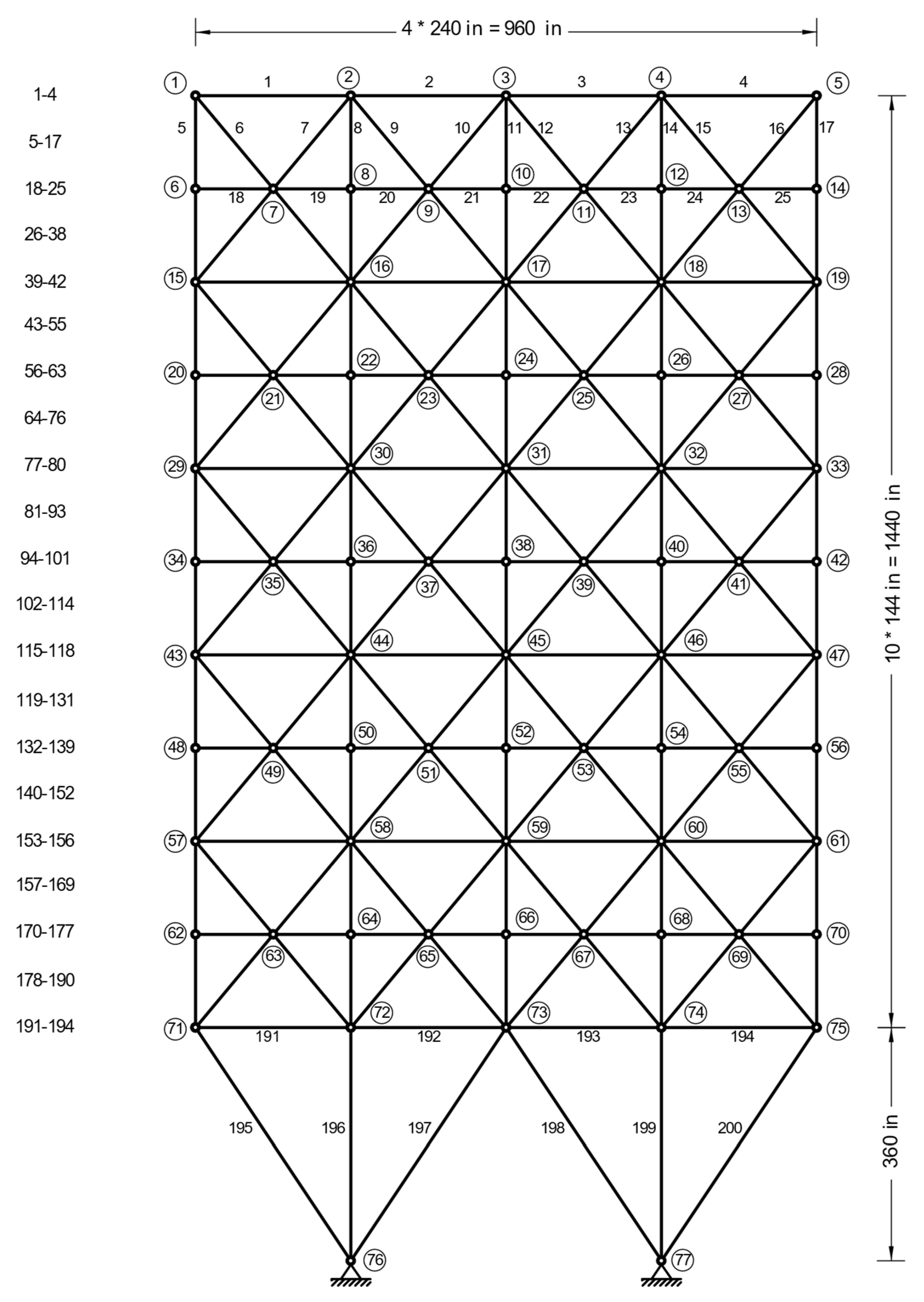
4.3. Two-Hundred-Bar Planar Truss Example

Figure 13 shows a 200-bar planar truss consisting of 77 joints connected by a total of 200 members. The 200 members were thoughtfully categorized into 29 independent groups. The selection of the cross-sectional areas of the truss members were chosen within the range of 0.1 to 2 in². The truss is designed with the sole consideration of the displacement constraints. The parameters used to optimize the design of this complex system are given in

Table 8. Design parameters of the 200-bar planar truss.

Parameter	Value
Modulus of elasticity	30,000 ksi
Material density	0.283 lb/in3
Allowable nodal displacement	4 in

. The joint loads applied on the truss are given in

Table 9. Applied loads on the 200-bar planar truss.

Joints	Px (kips)	Py (kips)	Pz (kips)
1, 6, 15, 20, 29, 34, 43, 48, 57, 62	1	0	0
1, 2, 3, 4, 5, 6, 8, 10, 12, 14, 15, 16, 17, 18, 19, 20, 22, 24, 26, 28, 29, 30, 31, 32, 33, 34, 36, 38, 40, 42, 43, 44, 45, 46, 47, 48, 50, 52, 54, 56, 57, 58, 59, 60, 61, 62, 64, 66, 68, 70, 71, 72, 73, 74, 75	0	−10	0

.

4.3.1. Data Preparation

Within a specified space of $\mathbf{A}\hspace{0.33em}\in \hspace{0.33em}[0.1,2]\hspace{0.33em} {\mathrm{in}}^2$, a structural design exploration was undertaken, generating 1000 truss design samples, each consisting of 29 design variables, with values randomly assigned within the specified range. The finite element model was used to analyze the structure, and from the resulting data, a graph-structured dataset was constructed. Due to the planar nature of the 200-bar truss, six distinct node features were adopted to represent the structure, as illustrated in Figure 14. The node features include truss joint coordinates $\left(x,\hspace{0.17em}y\right)$, joint loads $\left(F_x,\hspace{0.17em}{F}_y\right)$, and two binary features (0 or 1) indicating the degrees of freedom related to the translations of the joints. Moreover, each edge had a single cross-sectional area, A, feature. Also, each node has two nodal displacement output features $\left({\delta }_x,\hspace{0.17em}{\delta }_y\right)$ determined by FEM analysis.

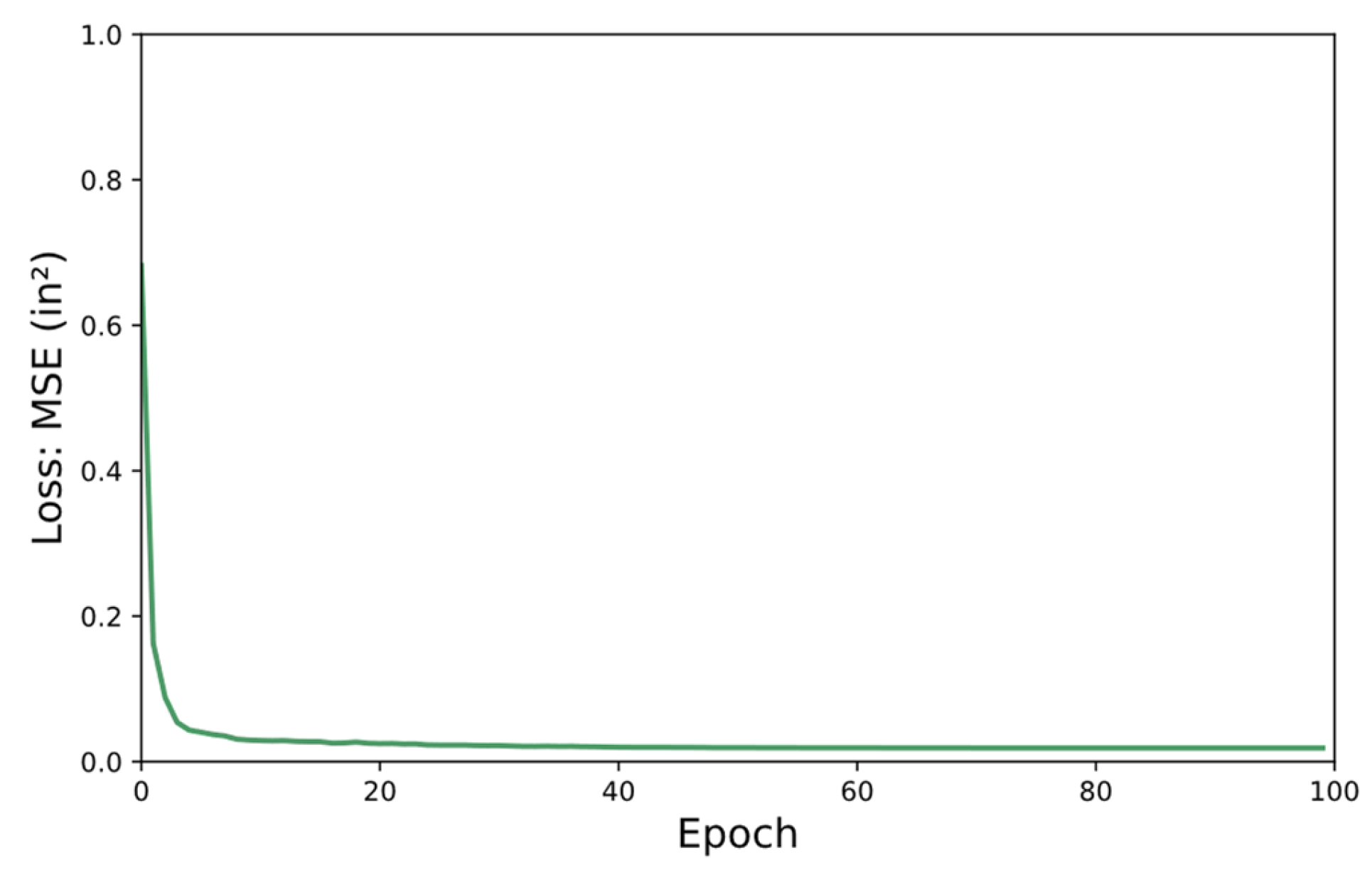
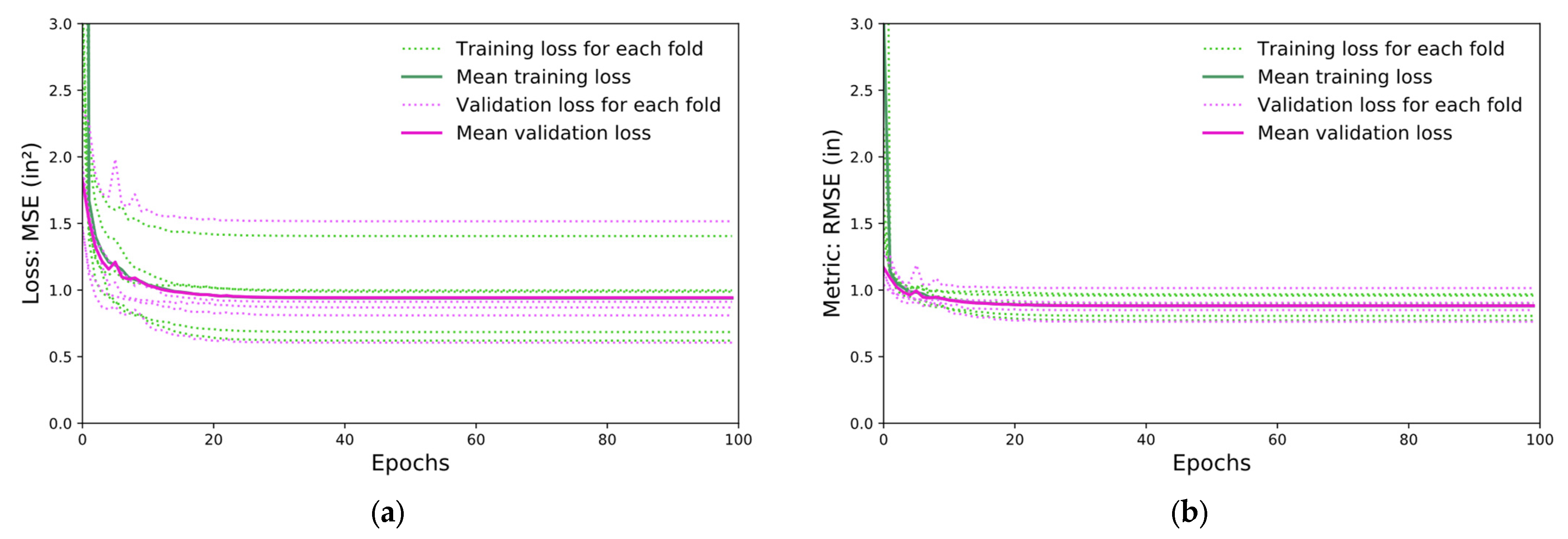
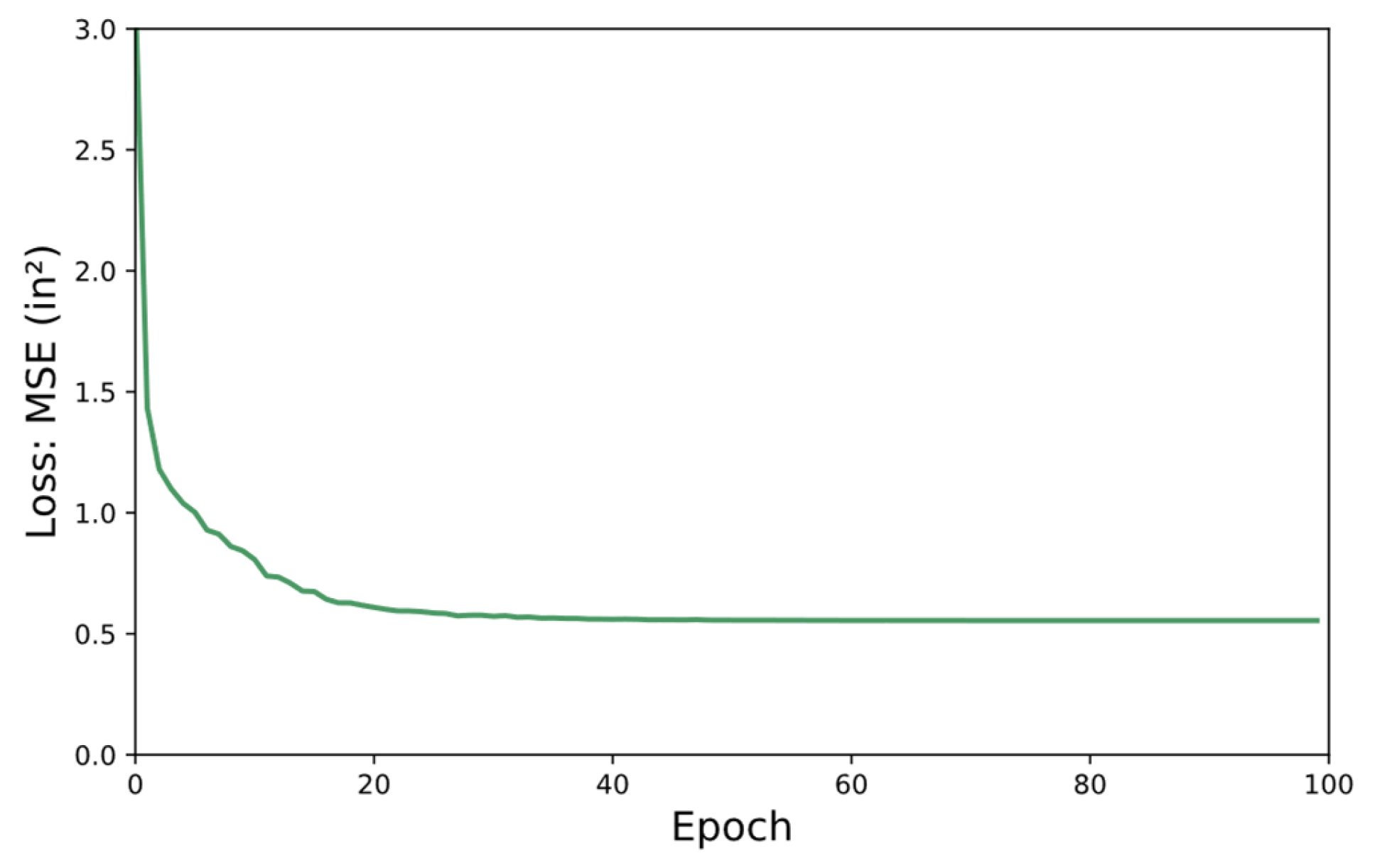
4.3.2. GNN Model Training

To evaluate the GNN model architecture, the five-fold cross-validation technique, as depicted in Figure 15, was implemented. The performance of the model was assessed by calculating the mean values of the MSE and RMSE for the training and validation datasets across the five folds. The values of MSE and RMSE are given in

Table 10. Mean results of five-fold cross-validation for 200-bar truss.

	Training	Validation
MSE (in2)	0.939	0.881
RMSE (in)	0.943	0.882

. To construct the surrogate model, the neural network was trained using all 1000 truss samples, resulting in a final mean square error of MSE = 0.496 in², as presented in Figure 16.

4.3.3. GNN-Based Optimization

The FEM-based optimization population remained constant at 75 across 150 iterations, while the population of the GNN-based optimization grew from 75 to 150 in the final 10% of iterations. The best outcome obtained from the 100 independent runs of both optimization techniques is presented in

Table 11. Optimal design for the 200-bar planar truss.

Variables		Cross-Sectional Areas (in2)
Element Group	Members	FEM-Based Optimization (Benchmark)	GNN-Based Optimization
1	1–4	0.100	0.100
2	5, 8, 11, 14, 17	0.435	0.523
3	19–24	0.100	0.100
4	18, 25, 56, 63, 94, 101, 132, 139, 170, 177	0.100	0.100
5	26, 29, 32, 35, 38	0.660	0.586
6	6, 7, 9, 10, 12, 13, 15, 16, 27, 28, 30, 31, 33, 34, 36, 37	0.100	0.100
7	39–42	0.100	0.100
8	43, 46, 49, 52, 55	0.754	0.855
9	57–62	0.100	0.100
10	64, 67, 70, 73, 76	0.925	0.802
11	44, 45, 47, 48, 50, 51, 53, 54, 65, 66, 68, 69, 71, 72, 74, 75	0.100	0.100
12	77–80	0.100	0.100
13	81, 84, 87, 90, 93	0.929	0.910
14	95–100	0.100	0.100
15	102, 105, 108, 111, 114	1.135	1.095
16	82, 83, 85, 86, 88, 89, 91, 92, 103, 104, 106, 107, 109, 110, 112, 113	0.100	0.100
17	115–118	0.100	0.100
18	119, 122, 125, 128, 131	1.220	1.065
19	133–138	0.100	0.100
20	140, 143, 146, 149, 152	1.240	1.162
21	120, 121, 123, 124, 126, 127, 129, 130, 141, 142, 144, 145, 147, 148, 150, 151	0.100	0.100
22	153–156	0.100	0.100
23	157, 160, 163, 166, 169	1.434	1.816
24	171–176	0.100	0.100
25	178, 181, 184, 187, 190	1.446	1.619
26	158, 159, 161, 162, 164, 165, 167, 168, 179, 180, 182, 183, 185, 186, 188, 189	0.133	0.116
27	191–194	0.839	0.823
28	195, 197, 198, 200	1.497	1.496
29	196, 199	2.000	2.000
${\left|{\delta }_{node}\right|}^{\max }$(in)		4.00	4.00
Weight (lb)		4166.81	4204.00
Nanalyses		11,250	3750

. As can be seen, in comparison to the outcome of the FEM-based optimization, the achieved optimal structural weight using the GNN-based optimization displays a high accuracy with a minimal difference of 0.9%. The GNN-based technique took only 607.1 s for predictions, which included 80.5 s and 526.6 s for the data preparation and the optimization stages, respectively. On the other hand, the FEM-based technique required an average of 731.5 s with 11,250 analyses to solve the problem, which was a significantly longer computational time compared to the GNN-based technique.

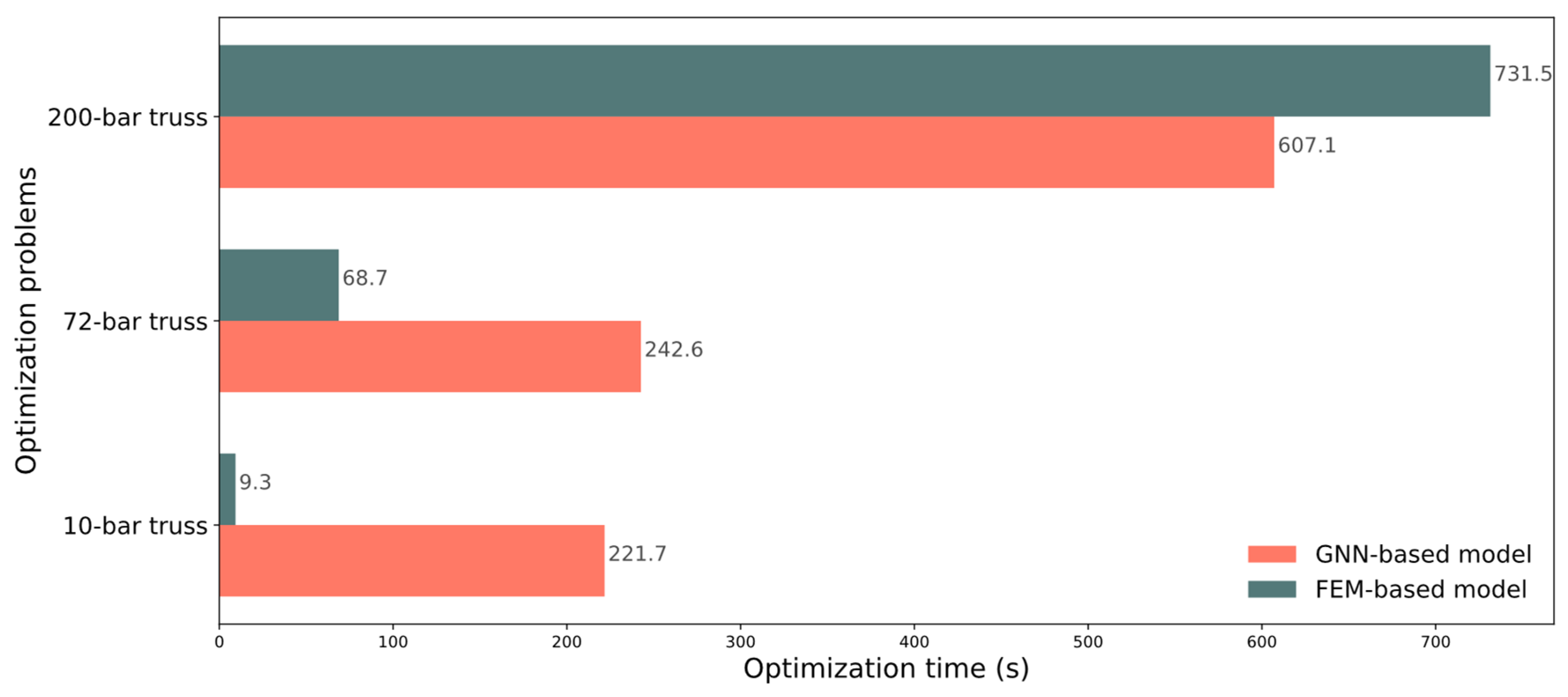
4.4. Accuracy and Effectiveness

The comparative analysis of the two optimization techniques, namely, the proposed GNN-based and the conventional FEM-based, presented in Section 4.1,Section 4.2 and Section 4.3 has demonstrated the accuracy and effectiveness of the developed GNN-based optimization in solving three distinct truss design problems. The results of the study reveal that the GNN-based optimization technique can find the optimal weights with a remarkable degree of accuracy without violating any constraints. Specifically, the achieved optimal weights are characterized by only a marginal deviation of 0.05%, 0.2%, and 0.9% from the results of the FEM-based optimization for the 10-bar planar truss, 72-bar space truss, and 200-bar planar truss, respectively. In addition to its high accuracy, the GNN-based optimization exhibits a higher degree of efficiency for more complex structures compared to the FEM-based optimization. This is evident from Figure 17, which shows that the GNN-based optimization was able to reach the optimal results faster for the 200-bar planar truss problem, outperforming the FEM-based optimization, which identified the optimal weights for the 10-bar planar truss and the 72-bar space truss problems more expeditiously.

5. Summary, Conclusions, and Future Work

In this study, a novel graph neural network (GNN)-based optimization technique is proposed for dealing with the size optimization of truss structures. The technique employs a particle swarm optimization algorithm to conduct an iterative search for the optimal solutions. A surrogate model based on a graph neural network is trained to approximate the nodal displacements of trusses with different sets of cross-sectional areas of the truss elements for the first 90% of iterations, while the remaining 10% utilizes FEM analysis to determine accurate nodal displacements. In this manner, this technique eliminates the need for finite element models to analyze truss structures, which in turn leads to computational time reduction. Moreover, three different truss optimization problems, a 10-bar truss, a 72-bar truss, and a 200-bar truss, are used to investigate the proposed GNN-based optimization technique against a conventional FEM-based technique. The results demonstrate the superiority of the GNN-based technique, as it arrives at the optimal design with no constraint violations and is faster in complex truss structures like the 200-bar problem.

There are two avenues for future improvement in this research. Firstly, enhancing the surrogate model by incorporating a trained GNN to predict the stresses in the truss elements alongside the nodal displacements. Secondly, training a single GNN to predict the structural response of trusses of different topologies, paving the way to the simultaneous optimization of truss topology and size.

References

1. Horta, I.M.; Camanho, A.S.; Johnes, J.; Johnes, G. Performance trends in the construction industry worldwide: An overview of the turn of the century. J. Product. Anal. 2013, 39, 89–99. [Google Scholar] [CrossRef]
2. Mei, L.; Wang, Q. Structural Optimization in Civil Engineering: A Literature Review. Buildings 2021, 11, 66. [Google Scholar] [CrossRef]
3. Kaveh, A.; Khayatazad, M. Ray Optimization for Size and Shape Optimization of Truss Structures. Comput. Struct. 2013, 117, 82–94. [Google Scholar] [CrossRef]
4. Dorn, W.; Gomory, R.; Greenberg, H.J. Automatic Design of Optimal Structures. J. Mec. 1964, 3, 25–52. [Google Scholar]
5. Hajela, P.; Lee, E. Genetic algorithms in truss topological optimization. Int. J. Solids Struct. 1995, 32, 3341–3357. [Google Scholar] [CrossRef]
6. Wang, D.; Zhang, W.H.; Jiang, J.S. Truss shape optimization with multiple displacement constraints. Comput. Methods Appl. Mech. Eng. 2002, 191, 3597–3612. [Google Scholar] [CrossRef]
7. Miguel, L.F.F.; Fadel Miguel, L.F. Shape and Size Optimization of Truss Structures Considering Dynamic Constraints through Modern Metaheuristic Algorithms. Expert Syst. Appl. 2012, 39, 9458–9467. [Google Scholar] [CrossRef]
8. Stolpe, M. Truss Optimization with Discrete Design Variables: A Critical Review. Struct. Multidiscip. Optim. 2016, 53, 349–374. [Google Scholar] [CrossRef]
9. Kaveh, A.; Malakouti Rad, S. Hybrid genetic algorithm and particle swarm optimization for the force method-based simultaneous analysis and design. Iran. J. Sci. Technol. Trans. B Eng. 2010, 34, 15–34. [Google Scholar]
10. Li, L.J.; Huang, Z.B.; Liu, F. A Heuristic Particle Swarm Optimization Method for Truss Structures with Discrete Variables. Comput. Struct. 2009, 87, 435–443. [Google Scholar] [CrossRef]
11. Renkavieski, C.; Parpinelli, R.S. Meta-heuristic algorithms to truss optimization: Literature mapping and application. Expert Syst. Appl. 2021, 182, 22. [Google Scholar] [CrossRef]
12. Saka, M.P.; Hasançebi, O.; Geem, Z.W. Metaheuristics in Structural Optimization and Discussions on Harmony Search Algorithm. Swarm Evol. Comput. 2016, 28, 88–97. [Google Scholar] [CrossRef]
13. Du, F.; Dong, Q.Y.; Li, H.S. Truss Structure Optimization with Subset Simulation and Augmented Lagrangian Multiplier Method. Algorithms 2017, 10, 128. [Google Scholar] [CrossRef] [Green Version]
14. Desale, S.; Rasool, A.; Andhale, S.; Rane, P. Heuristic and Meta-Heuristic Algorithms and Their Relevance to the Real World: A Survey. Int. J. Comput. Eng. Res. Trends 2015, 2, 296–304. [Google Scholar]
15. Salehi, H.; Burgueño, R. Emerging Artificial Intelligence Methods in Structural Engineering. Eng. Struct. 2018, 171, 170–189. [Google Scholar] [CrossRef]
16. Flood, I. Towards the Next Generation of Artificial Neural Networks for Civil Engineering. Adv. Eng. Inform. 2008, 22, 4–14. [Google Scholar] [CrossRef]
17. Lee, S.; Ha, J.; Zokhirova, M.; Moon, H.; Lee, J. Background Information of Deep Learning for Structural Engineering. Arch. Comput. Methods Eng. 2018, 25, 121–129. [Google Scholar] [CrossRef]
18. Gu, G.X.; Chen, C.T.; Buehler, M.J. De Novo Composite Design Based on Machine Learning Algorithm. Extrem. Mech. Lett. 2018, 18, 19–28. [Google Scholar] [CrossRef]
19. Nguyen, H.; Vu, T.; Vo, T.P.; Thai, H.T. Efficient Machine Learning Models for Prediction of Concrete Strengths. Constr. Build. Mater. 2021, 266, 17. [Google Scholar] [CrossRef]
20. Abueidda, D.W.; Koric, S.; Sobh, N.A. Topology Optimization of 2D Structures with Nonlinearities Using Deep Learning. Comput. Struct. 2020, 237, 14. [Google Scholar] [CrossRef]
21. Kollmann, H.T.; Abueidda, D.W.; Koric, S.; Guleryuz, E.; Sobh, N.A. Deep Learning for Topology Optimization of 2D Metamaterials. Mater. Des. 2020, 196, 14. [Google Scholar] [CrossRef]
22. Yu, Y.; Hur, T.; Jung, J.; Jang, I.G. Deep Learning for Determining a Near-Optimal Topological Design without any Iteration. Struct. Multidiscip. Optim. 2019, 59, 787–799. [Google Scholar] [CrossRef] [Green Version]
23. Chandrasekhar, A.; Suresh, K. TOuNN: Topology Optimization Using Neural Networks. Struct. Multidiscip. Optim. 2021, 63, 1135–1149. [Google Scholar] [CrossRef]
24. Moghadas, K.R.; Choong, K.K.; Bin Mohd, S. Prediction of Optimal Design and Deflection of Space Structures Using Neural Networks. Math. Probl. Eng. 2012, 2012, 712974. [Google Scholar]
25. Yücel, M.; Bekdaş, G.; Nigdeli, S.M. Prediction of Optimum 3-Bar Truss Model Parameters with an ANN Model. In Proceedings of the 6th International Conference on Harmony Search, Soft Computing and Applications, ICHSA 2020, Advances in Intelligent Systems and Computing, Istanbul, Turkey, 22–24 April 2020; Volume 1275, pp. 317–324. [Google Scholar]
26. Nguyen, T.-H.; Vu, A.-T. Prediction of Optimal Cross-Sectional Areas of Truss Structures Using Artificial Neural Networks. In Proceedings of the 6th International Conference on Geomatics, Civil Engineering and Structures, CIGOS 2021, Emerging Technologies and Applications for Green Infrastructure, Ha Long, Vietnam, 28–29 October 2021; Volume 203, pp. 1897–1905. [Google Scholar]
27. Nourian, N.; El-Badry, M.; Jamshidi, M. Design Optimization of Pedestrian Truss Bridges Using Deep Neural Network. In Proceedings of the 11th International Conference on Short and Medium Span Bridges, SMSB XI, Toronto, ON, Canada, 19–22 July 2022; p. 10. [Google Scholar]
28. Hajela, P.; Berke, L. Neurobiological computational models in structural analysis and design. Comput. Struct. 1991, 41, 657–667. [Google Scholar] [CrossRef]
29. Hajela, P.; Berke, L. Neural Network Based Decomposition in Optimal Structural Synthesis. Comput. Syst. Eng. 1991, 2, 473–481. [Google Scholar] [CrossRef]
30. Papadrakakis, M.; Lagaros, N.D.; Tsompanakis, Y. Optimization of Large-Scale 3-D Trusses Using Evolution Strategies and Neural Networks. Int. J. Space Struct. 1999, 14, 211–223. [Google Scholar] [CrossRef]
31. Liu, Y.; Lu, N.; Noori, M.; Yin, X. System Reliability-Based Optimisation for Truss Structures Using Genetic Algorithm and Neural Network. Int. J. Reliab. Saf. 2014, 8, 51–69. [Google Scholar] [CrossRef]
32. Zhou, Y.; Zhan, H.; Zhang, W.; Zhu, J.; Bai, J.; Wang, Q.; Gu, Y. A New Data-Driven Topology Optimization Framework for Structural Optimization. Comput. Struct. 2020, 239, 16. [Google Scholar] [CrossRef]
33. Nguyen, T.H.; Vu, A.T. Using Neural Networks as Surrogate Models in Differential Evolution Optimization of Truss Structures. In Proceedings of the 12th International Conference on Computational Collective Intelligence, ICCCI 2020, Da Nang, Vietnam, 30 November–3 December 2020; Volume 12496, pp. 152–163. [Google Scholar]
34. Mai, H.T.; Kang, J.; Lee, J. A Machine Learning-Based Surrogate Model for Optimization of Truss Structures with Geometrically Nonlinear Behavior. Finite Elem. Anal. Des. 2021, 196, 14. [Google Scholar] [CrossRef]
35. Gori, M.; Monfardini, G.; Scarselli, F. A New Model for Learning in Graph Domains. In Proceedings of the 2005 IEEE International Joint Conference on Neural Networks, Montreal, QC, Canada, 31 July–4 August 2005; Volume 2, pp. 729–734. [Google Scholar]
36. Scarselli, F.; Hagenbuchner, M.; Yong, S.L.; Tsoi, A.C.; Gori, M.; Maggini, M. Graph Neural Networks for Ranking Web Pages. In Proceedings of the 2005 IEEE/WIC/ACM International Conference on Web Intelligence, WI’05, Compiegne, France, 19–22 September 2005; pp. 666–672. [Google Scholar]
37. Li, Y.; Tarlow, D.; Brockschmidt, M.; Zemel, R. Gated Graph Sequence Neural Networks. In Proceedings of the International Conference on Learning Representations, ICLR 2016, San Juan, Puerto Rico, 2–4 May 2016; p. 20. [Google Scholar]
38. Bronstein, M.M.; Bruna, J.; Lecun, Y.; Szlam, A.; Vandergheynst, P. Geometric Deep Learning: Going beyond Euclidean Data. IEEE Signal Process Mag. 2017, 34, 18–42. [Google Scholar] [CrossRef] [Green Version]
39. Zhang, S.; Tong, H.; Xu, J.; Maciejewski, R. Graph Convolutional Networks: A Comprehensive Review. Comput. Soc. Netw. 2019, 6, 23. [Google Scholar] [CrossRef] [Green Version]
40. Wu, Z.; Pan, S.; Chen, F.; Long, G.; Zhang, C.; Yu, P.S. A Comprehensive Survey on Graph Neural Networks. IEEE Trans. Neural Netw. Learn. Syst. 2021, 32, 4–24. [Google Scholar] [CrossRef] [Green Version]
41. Chami, I.; Abu-El-Haija, S.; Perozzi, B.; Ré, C.; Murphy, K. Machine Learning on Graphs: A Model and Comprehensive Taxonomy. J. Mach. Learn. Res. 2022, 23, 3840–3903. [Google Scholar]
42. Zhang, Z.; Cui, P.; Zhu, W. Deep Learning on Graphs: A Survey. IEEE Trans. Knowl. Data Eng. 2022, 34, 249–270. [Google Scholar] [CrossRef] [Green Version]
43. Duvenaud, D.; Maclaurin, D.; Aguilera-Iparraguirre, J.; Gómez-Bombarelli, R.; Hirzel, T.; Aspuru-Guzik, A.; Adams, R.P. Convolutional Networks on Graphs for Learning Molecular Fingerprints. In Proceedings of the 28th International Conference on Neural Information Processing Systems, NIPS’15, Montreal, QC, Canada, 7–12 December 2015; Volume 2, pp. 2224–2232. [Google Scholar]
44. Hamaguchi, T.; Oiwa, H.; Shimbo, M.; Matsumoto, Y. Knowledge Transfer for Out-of-Knowledge-Base Entities: A Graph Neural Network Approach. In Proceedings of the 26th International Joint Conference on Artificial Intelligence, IJCAI 2017, Melbourne, Australia, 19–25 August 2017; p. 7. [Google Scholar]
45. Battaglia, P.; Pascanu, R.; Lai, M.; Rezende, D.J. Interaction Networks for Learning about Objects, Relations and Physics. In Proceedings of the 29th International Conference on Neural Information Processing Systems, NIPS’16, Barcelona, Spain, 5–10 December 2016; p. 9. [Google Scholar]
46. Maurizi, M.; Gao, C.; Berto, F. Predicting stress, strain and deformation fields in materials and structures with graph neural networks. Sci. Rep. 2022, 12, 21834. [Google Scholar] [CrossRef]
47. Battaglia, P.W.; Hamrick, J.B.; Bapst, V.; Sanchez-Gonzalez, A.; Zambaldi, V.; Malinowski, M.; Tacchetti, A.; Raposo, D.; Santoro, A.; Faulkner, R.; et al. Relational inductive biases, deep learning, and graph networks. arXiv 2018, arXiv:1806.01261. [Google Scholar]
48. Kingma, D.P.; Ba, J. Adam: A Method for Stochastic Optimization. In Proceedings of the International Conference on Learning Representations, ICLR 2015, San Diego, CA, USA, 7–9 May 2015; p. 15. [Google Scholar]
49. Grattarola, D.; Alippi, C. Graph Neural Networks in TensorFlow and Keras with Spektral. IEEE Comput. Intell. Mag. 2021, 16, 99–106. [Google Scholar] [CrossRef]
50. Zhou, J.; Cui, G.; Hu, S.; Zhang, Z.; Yang, C.; Liu, Z.; Wang, L.; Li, C.; Sun, M. Graph Neural Networks: A Review of Methods and Applications. AI Open 2020, 1, 57–81. [Google Scholar] [CrossRef]
51. Simonovsky, M.; Komodakis, N. Dynamic Edge-Conditioned Filters in Convolutional Neural Networks on Graphs. In Proceedings of the 2017 IEEE Conference on Computer Vision and Pattern Recognition, CVPR, Honolulu, HI, USA, 21–26 July 2017; pp. 3693–3702. [Google Scholar]
52. Xie, T.; Grossman, J.C. Crystal Graph Convolutional Neural Networks for an Accurate and Interpretable Prediction of Material Properties. Phys. Rev. Lett. 2018, 120, 6. [Google Scholar] [CrossRef] [Green Version]
53. Kennedy, J.; Eberhart, R. Particle Swarm Optimization. In Proceedings of the International Conference on Neural Networks, ICNN’95, Perth, Australia, 27 November–1 December 1995; Volume 4, pp. 1942–1948. [Google Scholar]
54. Kennedy, J.; Eberhart, R.C. Swarm Intelligence; Elsevier: Amsterdam, The Netherlands, 2001. [Google Scholar]
55. Liang, J.J.; Qin, A.K.; Suganthan, P.N.; Baskar, S. Comprehensive Learning Particle Swarm Optimizer for Global Optimization of Multimodal Functions. IEEE Trans. Evol. Comput. 2006, 10, 281–295. [Google Scholar] [CrossRef]
56. Shi, Y.; Eberhart, R. Modified Particle Swarm Optimizer. In Proceedings of the 1998 IEEE International Conference on Evolutionary Computation, ICEC, Anchorage, AK, USA, 4–9 May 1998; pp. 69–73. [Google Scholar]
57. Rajeev, B.S.; Krishnamoorthy, C.S. Discrete Optimization of Structures Using Genetic Algorithms. J. Struct. Eng. 1992, 118, 1233–1250. [Google Scholar] [CrossRef]
58. Jawad, F.K.J.; Mahmood, M.; Wang, D.; AL-Azzawi, O.; Al-Jamely, A. Heuristic Dragonfly Algorithm for Optimal Design of Truss Structures with Discrete Variables. Structures 2021, 29, 843. [Google Scholar] [CrossRef]
Figure 1. Flowchart illustrating the GNN-based truss size optimization.
Algorithms 16 00380 g001
Figure 2. Directed and undirected edges.
Algorithms 16 00380 g002
Figure 3. A typical GNN model.
Algorithms 16 00380 g003
Figure 4. Encode-Process-Decode architecture.
Algorithms 16 00380 g004
Figure 5. Ten-bar planar truss.
Algorithms 16 00380 g005
Figure 6. Graph representation of the 10-bar planar truss.
Algorithms 16 00380 g006
Figure 7. (a) Convergence history of the loss function for five-fold validation model; and (b) convergence history of the metric function for five-fold validation model.
Algorithms 16 00380 g007
Figure 8. Convergence history of the loss function for the trained surrogate model.
Algorithms 16 00380 g008
Figure 9. Seventy-two-bar space truss.
Algorithms 16 00380 g009
Figure 10. Graph representation of the 72-bar space truss.
Algorithms 16 00380 g010
Figure 11. (a) Convergence history of the loss function for five-fold validation model; and (b) convergence history of the metric function for five-fold validation model.
Algorithms 16 00380 g011
Figure 12. Convergence history of the loss function for the trained surrogate model.
Algorithms 16 00380 g012
Figure 13. The 200-bar planar truss.
Algorithms 16 00380 g013
Figure 14. Graph representation of the 200-bar planar truss.
Algorithms 16 00380 g014
Figure 15. (a) Convergence history of the loss function for five-fold validation model; and (b) convergence history of the metric function for five-fold validation model.
Algorithms 16 00380 g015
Figure 16. Convergence history of the loss function for the trained surrogate model.
Algorithms 16 00380 g016
Figure 17. Optimization process time for the GNN-based and FEM-based techniques.
Algorithms 16 00380 g017