Article

Basis Functions for a Transient Analysis of Linear Commensurate Fractional-Order Systems

1
Department of Electrical Engineering, University of Defence Brno, 662 10 Brno, Czech Republic
2
Department of Radio Electronics, Brno University of Technology, 616 00 Brno, Czech Republic
*
Author to whom correspondence should be addressed.
Algorithms 2023, 16(7), 335; https://doi.org/10.3390/a16070335
Submission received: 25 May 2023 / Revised: 5 July 2023 / Accepted: 11 July 2023 / Published: 13 July 2023
(This article belongs to the Collection Feature Papers in Algorithms for Multidisciplinary Applications)

Abstract

:
In this paper, the possibilities of expressing the natural response of a linear commensurate fractional-order system (FOS) as a linear combination of basis functions are analyzed. For all possible types of sα-domain poles, the corresponding basis functions are found, the kernel of which is the two-parameter Mittag–Leffler function Eα,β, β = α. It is pointed out that there are mutually unambiguous correspondences between the basis functions of FOS and the known basis functions of the integer-order system (IOS) for α = 1. This correspondence can be used to algorithmically find analytical formulas for the impulse responses of FOS when the formulas for the characteristics of IOS are known. It is shown that all basis functions of FOS can be generated with Podlubny‘s function of type εk (t, c; α, α), where c and k are the corresponding pole and its multiplicity, respectively.

1. Introduction

The zero-input response, sometimes also referred to as the natural response, is a well-known concept in system theory. It is the response of a system to its initial conditions, represented by the vector of the initial state in the absence of external excitation. The second well-known component of a system motion is its zero-state response, or forced response, which is the response of the system to external excitation under zero initial conditions. For linear systems, as a consequence of the superposition principle, the total response of the system, i.e., its response to external excitation under general initial conditions, is the sum of the zero-input and zero-state response [1].
The natural response plays a specific role in describing phenomena in systems left “to themselves”. From the way these systems deal with their own initial conditions and how the corresponding movement of the system can be observed through the chosen outputs, one can infer the stability of the system and the observability of the corresponding state variables from these outputs. The zero-state response, in turn, indicates the way in which signals from given inputs are propagated to given outputs through the state dynamics.
Furthermore, it is well known that the natural response of a linear system can be composed of a linear combination of so-called basis functions [2]. If a linear differential system with lumped parameters is considered, then the corresponding basis functions are components of the general solution of the corresponding input–output homogeneous differential equation of the system. The same basis functions appear in the general solution of the set of state equations of the system at zero excitation. The basis functions of a particular system are uniquely determined by the system poles, i.e., by the roots of its corresponding characteristic equation or the eigenvalues of the state matrix.
For classical integer-order systems (IOSs), the possible basis functions are functions of the form eat, sin(bt), cos(bt) and their combinations eat sin(bt), eat cos(bt), which are further multiplied by the functions tk, k = 0, 1, ..., m − 1, m ∈ N, a ∈ R, b ∈ R+ in the case of m-tuple poles. All these basis functions can be expressed by the real and imaginary components of the exponential function of the complex argument, which will be hereinafter referred to as the generating basis function f ∈ C:
f ( t ) = t k e ( a + i b ) t .
The above basis functions play an important role in the concept of modes of motion of a linear system [3], which is known from classical mechanics [4]. The linear combination of the basis functions can be used to model not only the natural response, but also selected types of forced responses, which include the impulse responses of so-called proper systems, i.e., systems of an integer order whose transfer functions have a polynomial of a lower order in the numerator than in the denominator. In the opposite case of improper systems, the impulse response contains, in addition to the basis functions mentioned above, the Dirac impulses and their derivatives, which penetrate the output due to the Dirac impulse exciting the system input.
The concept of basis functions can be extended to the class of linear fractional-order systems (FOSs). It is well known that the Mittag–Leffler functions (MLFs) with one, two or three parameters play an important role in the description of these systems, and can thus be viewed as a generalization of the classical exponential function from the domain of IOS [5]. It can be therefore expected that basis functions from the world of FOS are a generalization of the above basis functions and thus they could be derived from some known kinds of the MLFs. On the other hand, the MLFs are not the only possible candidates: for example, several different definitions of exponential and goniometric functions generalized to the fractional domain are known [6,7,8,9,10,11]. Dictionaries of the Laplace transform for a fractional domain include functions such as Dawson, erc, ercf, Bessel, extended Bessel, hypergeometric, Hermite polynomials [12] or, for example, the function introduced by Podlubny in [13] for solving fractional differential equations. It is necessary to consider which of these or similar functions are appropriate to be selected for the set of basis functions. Furthermore, one should analyze the modification of these functions for the case of multiple poles and try to find an equivalent to the above function tk for FOS. The notional culmination of this work should be to find a generating basis function from which all basis functions for the fractional domain can be generated, i.e., an analogue of function (1) for the integer-order domain.
The concept of basis functions can be used to algorithmically generate equations of waveforms of system responses via an analysis program. For example, formulas of responses to initial conditions or impulse or step responses as functions of time can be generated. The Laplace transform of the response, for example, the transfer function as the Laplace transform of the impulse response, is decomposed into partial fractions. A basis function of time is assigned to each fraction. The impulse response is then expressed as a linear combination of the basis functions. Once the basis functions are quantified, the waveform of the corresponding response is directly obtained with an algebraic evaluation, not with a classical numerical solution of differential equations. The accuracy of the result is determined with the accuracy of the pole calculation, the accuracy of the algorithm of partial fraction decomposition and the accuracy in computing the basis functions. This procedure also has the advantage of offering insight into the dynamics of the system through the analytical formula of the response. Simulation programs for a so-called symbolic and semi-symbolic circuit analysis work on this principle [14].
As far as numerical methods for calculating the standard responses of linear systems are concerned, particularly the impulse or step responses, either standard simulation programs such as SPICE or another platform for scientific and technical calculations such as MATLAB can be used. Of course, programs like MATLAB also allow an analysis using various numerical algorithms that are not available in classical simulation programs [15,16]. A review of numerical methods for solving linear fractional differential equations and a discussion of specific problems associated with them are given in [17]. Additional procedures are published in [15] together with codes for implementation in MATLAB. The method based on closed-form solutions to linear fractional-order differential equations starts from the approximate Grünwald–Letnikov definition of the fractional-order derivative. However, the accuracy of the transient analysis strongly depends on the choice of the computational step, so the method is of little use when solving practical problems. In [18], a generalization of the classical integer-order integrator approach for the numerical solution of the free (zero-input) response is made by elaborating the concept of the fractional integrator. In [19], the concept of LFD (Local Fractional Derivative) is used to compute zero-input responses.
Numerical algorithms of the Laplace inversion can also be used for a transient analysis [20,21]. An excellent discussion of the selected algorithms is given in [22,23].
Procedures utilizing analytical preprocessing of results are also popular. The analytical solution of a linear homogeneous fractional-order differential equation was first published in the classic work [13]. However, the corresponding formula contains infinite sums of derivatives of two-parameter MLFs, and is thus of little use for practical calculations.
Interesting possibilities of a transient analysis are offered for the so-called commensurate systems, where all non-integer powers of the operator s in their transfer functions are rational numbers. For commensurate systems, one can use a procedure leading to expressing their impulse or step responses in terms of a finite sum of MLFs [15,24,25].
The algorithmic generation of waveform formulas, constructed from basis functions, is an interesting alternative to the above numerical methods because it completely eliminates the numerical solution of differential equations of a non-integer order.
The above summary of the state of the art indicates the usefulness of extending the concept of basis functions to the domain of linear fractional-order systems. In the following section, the problem to be solved is specified, and new pieces of knowledge arising from its solution as well as their application potential are pointed out.

2. Problem Formulation

The purpose of this article is to solve the following problem:
Consider a linear time-invariant IOS, described with a proper s plane transfer function
K ( s ) = i = 0 m b i s i i = 0 n a i s i ,
where ai, bi ∈ R, an ≠ 0, m, n ∈ N+ and m < n.
Let us define an associated commensurate FOS with the transfer function KF, obtained from transfer function (2) by substituting
s s α , α R + ,
thus
K F ( s α ) = i = 0 m b i s α i i = 0 n a i s α i .
Denote the impulse responses of systems (2) and (4), i.e., the Laplace inverse of (2) and (4), as g(t) and gF(t), respectively.
Let us solve the following problem:
Suppose we know the analytic formula for g(t) as a linear combination of the basis functions of time. Let us find a procedure for deriving gF(t) from g(t) for all possible configurations of the coefficients ai, bi from (2) and (4), respectively.
It will be shown below that gF(t) can be obtained from g(t) such that to each known basis function of the IOS, the corresponding basis function of the FOS will be assigned. This result can be arrived at in the following steps: transfer function (1) will be decomposed into partial fractions, and each fraction will be converted into a basis function of time according to whether the corresponding pole is real or complex and simple or multiple. In the next step, substitution (2) will be applied to the formula of partial fraction decomposition, and the Laplace inversion will be used to arrive at the basis functions of associated system (3). By comparing the results from the two steps, we come to unambiguous correspondences between the basis functions in the integer-order and fractional-order domains.
The above procedure leads to the main contribution of this paper, which is the definition of a complete set of basis functions of commensurate FOS with transfer function (4). These functions allow an analytical description of the natural responses of all the above FOSs for an arbitrary set of their eigenvalues. This automatically implies the possible use of this analytical modeling for an accurate transient analysis of FOS without the need for a numerical solution of fractional-order differential equations, while the accuracy is guaranteed for both stable and unstable systems.
Another possible use arises from revealing the above correspondence between the basis functions of the FOS and the IOS: it can be used for an effective computer-aided transient analysis of commensurate FOSs with a direct utilization of the well-known algorithms for finding analytic formulas of responses of IOSs, with the proviso that in the final stage, the classical basis functions are replaced by new basis functions of associated FOS (3). In this paper, we will point out another interesting use of the formulas of impulse responses of FOS constructed from basis functions: reflecting them back into the space of IOSs, one can arrive at hitherto unpublished or little-known correspondences between the Laplace transforms and their time-domain representations from the world of classical IOS.
This paper is structured as follows: in Section 3, following this section, the mathematical prerequisites for constructing the basis functions are summarized. In Section 4 and Section 5, the Laplace inversions of the transfer function of a commensurate proper FOS for real and complex, single and multiple poles are performed with the aim of expressing the corresponding basis functions in a unified way. Section 6 proposes the formalism for writing these functions and the function generating all the proposed basis functions, together with an unambiguous correspondence between the basis functions for IOS and FOS. Section 7 discusses the possibility of algorithmically expressing the analytical formulas for the step response from the knowledge of the formula of the impulse response composed of the basis functions. Section 8 discusses the numerical aspects of calculating the impulse and step responses with the method of generating their formulas from the transfer function. In Section 9, the procedures are demonstrated on examples.

3. Mathematical Prerequisites

The purpose of this section is to summarize the mathematical prerequisites for analyzing to what extent certain functions known from fractional calculus are suitable candidates for their inclusion in the set of basis functions of a transient analysis.
This section has three objectives:
  • To summarize the well-known definitions of one-, two- and three-parameter MLFs of a complex argument, derivatives of two-parameter MLF and their interrelations, as well as relations with the classical exponential function.
  • To point out the possibility of expressing two-parameter MLFs of type Eα,β and their derivatives for the specific parameters α, β using functions of type Eα,α and their derivatives. This analysis will make it possible to verify the hypothesis that the set of basis functions can be reduced just to functions of type Eα,α and their derivatives.
  • To analyze the relations for real and imaginary parts of two-parameter MLFs and their derivatives, and the resulting appropriate definitions of fractional exponential functions and goniometric functions such as sine and cosine as potential building blocks of basis functions.

3.1. Mittag–Leffler Functions

The diagonal part of Table 1 summarizes the defining relations of the complex Mittag–Leffler functions of complex argument z: the classical MLF Eα (z) with one parameter α; the function Eα,β (z) with two parameters α, β; the m-th derivative of the function Eα,β (z) with respect to the argument z; and the function E α , β χ ( z ) with three parameters α, β, χ [5]. For completeness, the classical function exp(z) was added to the table and its known connections to MLFs are indicated.
In the legend to Table 1, it is recalled that the corresponding parameters α, β, χ may be complex with positive real parts [6]. In fractional calculus, the parameters in question often appear as positive integers.
It is obvious that the classical exponential function and the one-parameter and two-parameter MLFs are special cases of the three-parameter MLF, and that there is an unambiguous mapping between the integer derivatives of the two-parameter MLF and the three-parameter MLF. For χ = 1, the three-parameter MLF and its derivatives can be expressed in terms of the two-parameter MLF and its derivatives. A further analysis shows that the condition χ = 1 suffices for the construction of all variants of the formulas of the time responses of commensurate FOSs. While searching for basis functions, one can then focus on computationally simpler two-parameter MLFs.

3.2. Selected Relations between Two-Parameter Functions Eα,β, Eα,α and their Derivatives

Based on the analogy between the mathematical description of the response of classical and fractional systems, it is shown in Section 4 and Section 5 that it may be convenient to choose two-parameter MLFs of type Eα,α (z) and their derivatives as basis functions for a semi-symbolic analysis. At the same time, however, it turns out that the Laplace transforms of some waveforms lead to MLFs and their derivatives with a different distribution of parameters, namely to Eα,0 functions. Therefore, it may be useful to be able to transform these functions and their derivatives to Eα,α (z) functions and their derivatives.
However, the two-parameter MLF for the parameter β = 0, i.e., Eα,0 (z), contradicts the classical domain of MLF: β ∈ C, Re(β) > 0 [5]. The problem is that the gamma function, appearing in the defining relation of Eα,β (z), exhibits an infinite limit at 0. However, since the corresponding gamma function appears in the denominator of the defining relation of the two-parameter MLF, the first term of the infinite series defining the function Eα,β (z) is zero for β = 0 and k = 0. Then, the recurrence relation [26]
E α , β ( z ) = z E α , α + β ( z ) + 1 Γ ( β )
can be used to derive the identity
E α , 0 ( z ) = z E α , α ( z ) .
Numerical algorithms for computing the MLF available in [27,28,29], as well as the Wolfram Computational Notebook, for example, evaluate the function Eα,0 (z) in accordance with (6).
By successively differentiating both sides of (5), we arrive at a recurrence relation for the m-th derivative of the two-parameter MLF,
E α , β ( m ) ( z ) = z E α , α + β ( m ) ( z ) + m E α , α + β ( m 1 ) ( z ) , m > 0
whose solution is
E α , β ( m ) ( z ) = m ! z k = 0 m E α , α + β ( k ) ( z ) k ! .
Thus, for β = 0, arbitrary derivatives of the function Eα,0 (z) can be expressed using the derivatives of the function Eα,α (z):
E α , 0 ( m ) ( z ) = z E α , α ( m ) ( z ) + m E α , α ( m 1 ) ( z ) = m ! z k = 0 m E α , α ( k ) ( z ) k ! .
Note that the defining relation for the m-th derivative of the two-parameter function Eα,0 (z) exhibits no singularity for k = 0 when m > 0. Thus, the algorithms designed for this purpose [30,31] can be used directly for numerical computations of the derivatives of the function Eα,0 (z) even for β = 0.
It is worth noting that the robust algorithms for MLF computations [25,31] return correct results even for real parameters β < 0. The algorithm deals with the problem of infinite limits of the gamma function for the arguments −1, −2, −3, ... in the same way as for the argument of zero discussed above.
The fact that there is a clear relationship between the three-parameter MLF and the derivatives of the two-parameter MLF contributes to further possible narrowing of the set of basis functions. If an integer positive parameter χ = m + l, m ∈ N is substituted into the defining relation of the three-parameter MLF, then
E α , β m + 1 ( z ) = k = 0 ( m + 1 ) k k ! z k Γ ( α k + β ) = k = 0 ( m + k ) ! m ! k ! z k Γ ( α k + β ) .
After comparing the result with the definition of the m-th derivative of the two-parameter MLF, we find that [31]
E α , β m + 1 ( z ) = 1 m ! E α , β α m ( m ) ( z ) .
The back conversion, i.e., expressing the m-th derivative of the two-parameter MLF using the three-parameter MLF, is given in Table 1. This is to say that, for χ = m + l, m ∈ N, one can alternatively work with either one or the other type of basis functions as desired.
The above transformation relations are important not only from the methodological point of view (narrowing down the set of basis functions) but also from the point of view of numerical calculations, as will be discussed in Section 8.

3.3. Some Fractional Goniometric and Other Functions

In Section 4, we show that when computing some responses, it is convenient to compute the MLF as a complex function of the complex argument and, in a second step, to extract its real or imaginary part from the result. Consider the m-th derivative of a two-parameter MLF with complex argument z or complex conjugate z*,
z = x + i y = z e i φ , z * = x i y = z e i φ .
Then, the defining relation in Table 1 implies
E α , β ( m ) ( z ) = Re E α , β ( m ) ( z ) + i Im E α , β ( m ) ( z ) ,
E α , β ( m ) ( z * ) = Re E α , β ( m ) ( z ) i Im E α , β ( m ) ( z ) = E * α , β ( m ) ( z ) ,
E α , β ( m ) ( z ) + E α , β ( m ) ( z * ) = 2 Re E α , β ( m ) ( z ) ,
E α , β ( m ) ( z ) E α , β ( m ) ( z * ) = 2 i Im E α , β ( m ) ( z ) ,
where
Re E α , β ( m ) ( z ) = k = 0 ( k + m ) ! k ! z k cos ( k φ ) Γ ( α k + α m + β ) ,
Im E α , β ( m ) ( z ) = k = 0 ( k + m ) ! k ! z k sin ( k φ ) Γ ( α k + α m + β ) .
Although relations (15) and (16) are trivial, they are mentioned here since the real and imaginary parts of the corresponding MLFs and their derivatives described by these formulas play an important role in the semi-symbolic analysis of systems with complex poles (see Section 4).
The case of MLF with the purely imaginary argument z = iy, which corresponds to modeling the time response of a classical IOS without a damping factor, also deserves attention. In this case,
E α , β ( m ) ( i y ) = k = 0 ( k + m ) ! k ! i k y k Γ ( α k + α m + β ) = k = 0 ( 1 ) k ( 2 k + m ) ! ( 2 k ) ! y 2 k Γ ( ( 2 k + m ) α + β ) + i k = 0 ( 1 ) k ( 2 k + 1 + m ) ! ( 2 k + 1 ) ! y 2 k + 1 Γ ( ( 2 k + m + 1 ) α + β ) .
For the integer-order case, i.e., α = β = 1, the m-th derivative of the function Eα,β (iy) on the left-hand side of (19) translates into the classical exponential function of the imaginary argument, and the sums on the right-hand side translate into the Maclaurin series of functions of the cosine and sine type:
E 1 , 1 ( m ) ( i y ) = k = 0 ( 1 ) k ( 2 k + m ) ! ( 2 k ) ! y 2 k Γ ( 2 k + m + 1 ) + i k = 0 ( 1 ) k ( 2 k + 1 + m ) ! ( 2 k + 1 ) ! y 2 k + 1 Γ ( 2 k + m + 2 ) = k = 0 ( 1 ) k y 2 k ( 2 k ) ! + i k = 0 ( 1 ) k y 2 k + 1 ( 2 k + 1 ) ! = cos ( y ) + i sin ( y ) = e i y .
Thus, the sums on the right-hand side of (19) can be viewed as the m-th derivatives of the generalized (fractional) functions cosα,β (y) and sinα,β (y), and (19) can be rewritten in the form
E α , β ( m ) ( i y ) = cos α , β ( m ) ( y ) + i sin α , β ( m ) ( y ) ,
where
cos α , β ( m ) ( y ) = k = 0 ( 1 ) k ( 2 k + m ) ! ( 2 k ) ! y 2 k Γ [ ( 2 k + m ) α + β ] ,
sin α , β ( m ) ( y ) = k = 0 ( 1 ) k ( 2 k + m + 1 ) ! ( 2 k + 1 ) ! y 2 k + 1 Γ [ ( 2 k + m + 1 ) α + β ] .
The case m = 0 yields simple defining equations of fractional functions of the cosine and sine type:
cos α , β ( y ) = k = 0 ( 1 ) k y 2 k Γ ( 2 k α + β ) ,
sin α , β ( y ) = k = 0 ( 1 ) k y 2 k + 1 Γ [ ( 2 k + 1 ) α + β ] .
Formulas (24) and (25) are generalizations of one-parameter fractional functions of the cosine and sine type from [8,9] to two-parameter functions.
Relation (21) gives guidance on how to compute fractional functions (22) and (23) in a simple way: as real and imaginary parts of the derivatives of MLF with an imaginary argument.
Equation (21) as well as the identity E1,1 (z) = exp(z) confirm that the two-parameter MLF can be viewed as a generalization of the classical exponential function to the non-integer domain. Alternative definitions of the generalized exponential function of a non-integer order are published in [6,7,8,10]. Interesting for the purpose of a semi-symbolic analysis of fractional systems in the time domain is the following definition [7,8,10]:
e ˜ α , α ( a , t ) = t α 1 E α , α ( a t α ) , t > 0 ,
which can be formally extended to a two-parameter exponential function
e ˜ α , β ( a , t ) = t β 1 E α , β ( a t α ) , t > 0 .
Relations (26) and (27) are special cases of the function
ε k ( t , y ; α , β ) = t α k + β 1 E α , β ( k ) ( y t α )
introduced in [13], namely
e ˜ α , α ( a , t ) = ε 0 ( t , a ; α , α ) ,
e ˜ α , β ( a , t ) = ε 0 ( t , a ; α , β ) .
The definition of the two-parameter MLF implies the development of (27) into an infinite series
e ˜ α , β ( a , t ) = t β 1 k = 0 a t α k Γ ( α k + β ) .
From (31), it is easy to deduce that
e ˜ 1 , 1 ( a , t ) = e a t ,
e ˜ α , β ( i b , t ) = co s ˜ α , β ( b , t ) + i si n ˜ α , β ( b , t ) ,
where
co s ˜ α , β ( b , t ) = t β 1 k = 0 ( 1 ) k b t α 2 k Γ ( 2 α k + β ) ,
si n ˜ α , β ( b , t ) = t β 1 k = 0 ( 1 ) k b t α 2 k + 1 Γ ( 2 k + 1 ) α + β
are goniometric functions, associated with previously defined functions (24), (25) and (28) by the relations
co s ˜ α , β ( b , t ) = t β 1 cos α , β ( b t α ) = Re ε 0 ( t , i b ; α , β ) ,
si n ˜ α , β ( b , t ) = t β 1 sin α , β ( b t α ) = Im ε 0 ( t , i b ; α , β ) .
The Laplace transforms of exponential function (27) and goniometric functions (34) and (35) can be derived from (31), (34) and (35):
L e ˜ α , β ( a , t ) = s α β s α a ,
L co s ˜ α , β ( b , t ) = s 2 α β s 2 α + b 2 ,
L si n ˜ α , β ( b , t ) = b s α β s 2 α + b 2 .
In Section 5, we discuss the possibility of utilizing the above functions as basis functions for describing the transient responses of commensurate FOSs.

4. Time-Domain Response via Basis Functions: Real s1-Domain Poles

For the case of an m-tuple real pole s = a of the transfer function of an IOS, the corresponding partial fractions of decomposition (2) are of the familiar form
k = 1 m P k s a k
where Pk are the residues belonging to the root a.
The partial fractions of the decomposition of associated transfer function (4) of a commensurate FOS have the same form as (41), differing only in substitution (2), so they can be written as follows:
k = 1 m P k s α a k .
From the well-known formula
s δ s α a k t α k δ 1 ( k 1 ) ! E α , α δ ( k 1 ) ( a t α ) , k , δ N ; α R + ,
published in various notations in a number of works, e.g., [13], the relations can be derived between the time and Laplace domains, relevant to partial fractions (41) and (42), for single and multiple real poles, as shown in Table 2.
From a comparison of the relations in Table 2, analogies begin to emerge between the basis functions for IOS and FOS. For a simple pole, the classical exponential function of an IOS corresponds to a MLF of type Eα,α multiplied by a factor tα−1. However, this is a generalized exponential function (26). For the multiple pole, the classical exponential function is accompanied by a multiplicative term tk−1. In the fractional domain, this is reflected both by the derivative of the function Eα,α of order (k − 1) and by the multiplicative term tα(k−1). It is easy to see that the resulting waveform can then be smartly expressed by function (28) of type εk−1. A more detailed analysis will be carried out in Section 6.

5. Time-Domain Response via Basis Functions: Complex s1-Domain Poles

Consider that the transfer function K(s) in (1) contains an m-tuple complex conjugate pair of poles c, c*, where
c = a + ib, c* = a − ib.
The corresponding partial fractions of the decomposition of transfer function (2) can be written in the form
k = 1 n P k + s Q k ( s a ) 2 + b 2 k , P k , Q k R .
The k-th term of the associated transfer function of FOS (3) is
P k + s α Q k ( s α a ) 2 + b 2 k .
The following analysis is somewhat more complicated than for real poles. For the sake of clarity, it will be done separately for single and multiple poles.

5.1. Simple Complex Poles

For the case of simple poles (k = 1), (46) can be converted to the time domain using the following correspondence, published in [25]:
s δ ( s α a ) 2 + b 2 t α δ 1 b Im E α , α δ c t α , c = a + i b , b 0 ,
where Im denotes the imaginary part of the complex MLF.
By successively substituting σ = 0, σ = α into (47), Formula (46) can be converted to the time domain for k = 1 as follows:
P 1 + s α Q 1 ( s α a ) 2 + b 2 t α 1 b P 1 Im E α , α ( c t α ) + t 1 b Q 1 Im E α , 0 ( c t α ) .
Using (6) and (13)–(16), the right-hand side of (48) can be expressed using the functions Eα,α:
P 1 + s α Q 1 ( s α a ) 2 + b 2 t α 1 P 1 + Q 1 a b Im { E α , α ( c t α ) } + Q 1 Re { E α , α ( c t α ) } .
Equation (49) is the basic formula from which the various correspondences between the Laplace and time domains are derived in Table 3 for simple complex poles. The table shows that the classical waveforms of type exp(at)sin(bt) and exp(at)cos(bt) for IOS correspond to the combinations of basis functions of type tα−1 Im{Eα,α (ctα)} and tα−1 Re{Eα,α (ctα)} for FOS. In fact, these are the imaginary and real parts of fractional exponential function (26) with a complex argument.
Interesting results can be obtained for the Laplace transforms without a damping factor, i.e., with the parameter a = 0, which lead to undamped oscillations of type sin(bt) and cos(bt) for IOS. The corresponding fractional goniometric functions are sinα,α(btα) and cosα,α(btα) multiplied by the function tα−1. However, these are modified fractional goniometric functions (36) and (37).

5.2. Multiple Complex Poles

To convert partial fraction (46) into the time domain, one can proceed in a similar way as for the simple pole, but this time using the relation we published in [25]:
s δ [ ( s α a ) 2 + b 2 ] k A 1 0 ! t α δ 1 Im E α , α δ ( c t α ) A 2 1 ! t 2 α δ 1 Re E α , α δ ( 1 ) ( c t α ) + A 3 2 ! t 3 α δ 1 Im E α , α δ ( 2 ) ( c t α ) + A 4 3 ! t 4 α δ 1 Re E α , α δ ( 3 ) ( c t α ) A 5 4 ! t 5 α δ 1 Im E α , α δ ( 4 ) ( c t α ) A 6 5 ! t 6 α δ 1 Re E α , α δ ( 5 ) ( c t α ) = t α 1 i = 0 k 1 2 ( 1 ) i + 1 A 2 i + 1 t 2 i α δ ( 2 i ) ! Im E α , α δ ( 2 i ) ( c t α ) + t α 1 i = 0 k 2 1 ( 1 ) i + 1 A 2 ( i + 1 ) t ( 2 i + 1 ) α δ ( 2 i + 1 ) ! Re E α , α δ ( 2 i + 1 ) ( c t α )
where [x] denotes the integer part of x, and
A i = 2 ( 1 ) i 2 k i 1 k i 2 b ( 2 k i ) , i = 1 , 2 , , k .
Table 4 summarizes the Laplace transforms and their time representations (50) for the cases δ = 0, δ = α, and for the case of zero damping (a = 0). The responses for δ = α, which are expressed using the derivatives of the Eα,0 function according to (50), are adjusted to forms that use the Eα,α function via identity (9).
It can be seen from Table 4 that the classical basis functions of IOS of type exp(at)tk sin(bt) and exp(at)tk cos(bt) correspond to the imaginary and real parts of the k-th derivative of the function Eα,α multiplied by the functions tα−1 and tk. The k-th derivatives of the fractional functions of sine and cosine type (25) and (24) for β = α multiplied by the functions tα−1 and tk are assigned to the functions tk sin(bt) and tk cos(bt).
Note that the compact formulas of waveforms in the fractional domain obtained in this way after simplifying α = 1 directly yield the waveforms that correspond to the Laplace transforms for classical IOSs (see the “integer order” section of Table 4), which are not given even in the very detailed dictionaries of the Laplace transform [32].

6. Basis Functions for Integer- and Fractional-Order Commensurate Systems: One-to-One Correspondence

Starting from the possible forms of the decomposition of the transfer function into partial fractions for real and complex poles (41), (42), (46), and comparing the formulas of the corresponding waveforms for the IOS and FOS in Table 2, Table 3 and Table 4, we arrive at the summary of basis functions given in Table 5 in the “Basis Functions” columns. There are specific connections between these functions. These connections, which are different for single and multiple poles, are best seen by comparing the contents of the “Generated from” columns, which reveal from which general “generating function” these basis functions are generated.
Let us first compare the part of Table 5 for integer-order systems with the “Basis Functions” column for fractional-order systems.
If we restrict ourselves to simple poles, then the basis function eat of the IOS, i.e., the classical exponential function, corresponds to the basis function e ˜ α , α ( a , t ) of FOS, i.e., fractional exponential function (26). Undamped functions of the sine and cosine type are projected into the fractional domain as fractional sine and cosine functions of type (36) and (35).
Note that all of these above basis functions of FOS can be expressed using a two-parameter MLF of type Eα,α.
For multiple poles, the basis functions of IOS are given by the product of the integer power of time, tk, and the classical exponential function or its imaginary or real part. For FOS, they are the products of the non-integer powers of time tαk, the non-integer powers of time tα−1 and the k-th derivatives of the function Eα,α or its imaginary or real part. For the purely imaginary poles, the k-th derivatives of the functions sinα,α and cosα,α multiplied by the terms tα−1 correspond to the classical sine and cosine functions for IOS.
Note that all these basis functions of FOS for multiple poles can be expressed using the corresponding derivatives of the two-parameter MLF of type Eα,α.
Based on defining relation (28) for Podlubny’s function εk, it is easy to prove that all basis functions for the FOS, listed in the “Basis Functions” column, can be expressed just using the function εk as listed in the “Generated from” column.
Thus, Table 5 provides guidance on how to obtain the time response of a commensurate FOS from the response of the associated classical IOS, namely by substituting for each other the appropriate basis functions. The most systematic correspondence is provided by comparing the generating functions f(t) for IOS (1) and fF(t) for FOS,
f F ( t ) = ε k ( t , a + i b ; α , α )
(see the comparison of the “Generated from” columns in Table 5): for real poles of a general multiplicity, the basis functions are generated with the function tk eat or εk(t, a; α, α), and for complex poles of a general multiplicity, by the real and imaginary parts of the function tk e(a+ib)t or εk(t, a + ib; α, α).

7. Calculation of Step Response

The correspondence between the basis functions of the IOS and FOS from Table 5 allows a convenient determination of analytical formulas for the impulse response gF(t) of commensurate FOS from the known impulse response g(t) of IOS. Let us reiterate that transfer functions (2) and (4) of both systems are bounded by relation (3).
Let us analyze to what extent the correspondences of Table 5 can be used to determine the step response hF(t) of the FOS. Since the step response is the forced response to a unit step, the question is whether it can be constructed from the basis functions from Table 5, which describe natural, not forced, responses.
It turns out that in the general case, we really cannot make do with the above basis functions when constructing the step response.
The step response hF(t) of the associated commensurate FOS of transfer function KF(sα) (4) is obtained with the Laplace inversion of the function KF(sα)/s = K(sα)/s. Similarly, the step response h(t) of the IOS is the Laplace inverse of the expression K(s)/s:
h ( t ) = L 1 K ( s ) s , h F ( t ) = L 1 K ( s α ) s .
Since the denominator of the second equation contains the s operator, not its power sα, the assumption from Section 1 that the Laplace transform of the time response of a FOS is obtained from the Laplace transform of IOS with substitution (2) cannot be used. However, all the conclusions that follow from this assumption, including the transformation relations of Table 5, are based on this assumption.
On the other hand, the step response can be easily obtained with a direct integration of the impulse response with respect to time. Since the impulse response of proper systems can be thought of as a linear combination of basis functions, the step response is actually constructed from a linear combination of the integrals of the basis functions with respect to time. Using the rule of integration of Podlubny’s function (28) [13], the first integral of generating function fF (t) (52) can be written as follows:
f F ( t ) d t = ε k ( t , c ; α , α ) d t = ε k ( t , c ; α , α + 1 ) = t α k + α E α , α + 1 ( k ) ( c t α ) , c = a + i b .
Thus, it is obvious that the step response can be composed from the basis functions that are built of MLFs with the parameters α, α + 1. Starting from transfer function (4), it is possible to first determine the impulse response based on Table 5 and then proceed to the step response by integrating each basis function according to (54).

8. Numerical Aspects

Reliable algorithms for computing the basis functions are necessary for an accurate and fast computation of waveforms from their semi-symbolic formulas that use these functions.
Table 5 shows that all the basis functions for FOS can be uniformly generated with Podlubny’s function (28) εk(t, a + ib; α, α). In terms of numerical computations, it is a complex function of three real and one complex argument. Relation (28) defining this function contains the k-th derivative of the complex two-parameter MLF of the complex argument. The evaluation of this function can be approached either directly, i.e., with an algorithm for computing the derivatives of the two-parameter MLF, or indirectly by computing the three-parameter MLF, from which the derivatives of the two-parameter MLF can then be easily determined (see Table 1).
A number of papers deal with the numerical calculation of MLF. Some of them have become the basis for developing robust algorithms for evaluating two- and three-parameter MLFs [30,31]. Among the best known is the MATLAB function mlf.m of Podlubny and Kacenak [27], which computes the two-parameter MLF with a complex argument. However, since it is not designed to compute derivatives of MLFs, it cannot be used to compute the basis functions belonging to multiple poles. Garrappa’s ml.m function is available on the MATLAB Central File Exchange, allowing for computing one-parameter, two-parameter and three-parameter MLFs [29]. Thus, the ml.m function allows for computing the derivative of the two-parameter MLF indirectly, using three-parameter MLFs. The corresponding routine, which implements the optimal parabolic contour (OPC) algorithm described in [33], is based on the inversion of the Laplace transform on a parabolic contour suitably chosen in one of the regions of analyticity of the Laplace transform [29]. However, there are some limitations in computing three-parameter MLFs via the ml.m: the parameter α must be greater than 0 and less than 1, and the absolute value of the complex argument of the MLF must not be less than απ radians. In particular, the second condition can pose a significant limitation for computing derivatives of the two-parameter MLF as part of Podlubny’s generating function.
To evaluate two-parameter MLFs and their derivatives, it is convenient to use another MATLAB function, ml_deriv(α, β, k, z) by R. Garrappa. The function computes the k-th derivative of the MLF with the parameters α and β at each entry of the complex vector z. Derivatives of the ML function are evaluated by exploiting an algorithm combining (by means of the derivative balancing technique devised in [31]) the Taylor series, a summation formula based on the Prabhakar function and the numerical inversion of the Laplace transform obtained after generalizing the algorithm described in [33]. The function was successfully tested in [25] for the accuracy of computing the derivatives. Based on the results published in [25], the given algorithm was used to evaluate the basis functions of Table 5, which belong to all kinds of poles, real or complex, simple or with a general multiplicity. The algorithm from ml_deriv is also continuously implemented in the current versions of SNAP for symbolic, semi-symbolic and numerical analyses of analog fractional-order circuits [14].

9. Illustration of the Use of Basis Functions for Transient Analysis

The use of basis functions for a transient analysis is illustrated by two examples. In the first step, the formulas for impulse and step responses are always found. In the second step, these responses are quantified. The MATLAB script ml_deriv by R. Garrappa [25] was used to evaluate the basis functions.
The responses obtained with this procedure were also simulated in the following SPICE-family simulation programs: Cadence PSPICE 16.5, LTSpice XVII and Micro-Cap 12. The fractional-order transfer functions were modeled using Laplace sources. In case of inconsistent results, data from MATLAB were imported into the simulation program for comparison. The decision on which results were correct was made via the so-called FFT-check, i.e., by using the Fourier transform of the impulse responses and by comparing the results with the frequency characteristics derived from the transfer functions.
Significantly different outputs of SPICE-family programs when solving the same task were observed for all the simulations described below. It turned out that, in all cases, the correct results were generated only in MATLAB via the basis functions method. As far as SPICE-family programs are concerned, the most accurate analysis was achieved with Micro-Cap 12. For this reason, the Micro-Cap outputs were chosen for the MATLAB-SPICE comparison.

9.1. Minimum-Phase Fractional-Order System

A commensurate minimum-phase system is analyzed in [34], with the transfer function
K F ( s ) = i = 0 4 b i s i α i = 0 10 a i s i α , α = 1.2 ,
where
a0 = b0 = 750,000, a1 = 3,563,000, a2 = 6,433,000, a3 = 6,032,000, a4 = 3,357,000, a5 = 1,167,000, a6 = 251,620, a7 =
31,914, a8 = 2193, a9 = 75, a10 = 1, b1 = 690,000, b2 = 240,000, b3 = −26,000 and b4 = −4000.
For system (55), let us find the basis functions of its natural response and use them to construct the formulas for the impulse and step responses.
First, the basis functions and the impulse response of the associated IOS will be found. Substituting α = 1 into (55) yields the transfer function K(s) (see Equation (2)). The decomposition of K(s) into partial fractions and the Laplace inversion lead to the impulse response
g ( t ) = k = 1 6 P k e a k t + 2 e a 7 t P 7 r cos b 7 t P 7 i sin b 7 t + 2 e a 9 t P 9 r cos b 9 t P 9 i sin b 9 t .
Equation (56) implies that the transfer function K(s) has six real poles ak, k = 1... 6, and two pairs of complex conjugate poles of type ck = ak ± ibk. The corresponding residues are denoted by the symbols Pk = Pkr + iPki. The poles and residues were calculated with a high precision using the MATLAB symbolic toolbox, and, after rounding, they are summarized in Table 6.
A similar decomposition of the function K(s)/s can be used to obtain the formula for the step response.
Based on (56) and Table 6, the formula of the impulse response of the associated commensurate system with transfer function KF (s) (55) can be directly written as
g F ( t ) = k = 1 6 P k ε 0 ( t , a k ; α , α ) + 2 P 7 r Re ε 0 ( t , c 7 ; α , α ) P 7 i Im ε 0 ( t , c 7 ; α , α ) + P 9 r Re ε 0 ( t , c 9 ; α , α ) P 9 i Im ε 0 ( t , c 9 ; α , α )
The step response is easily determined from (57) using (54):
h F ( t ) = k = 1 6 P k ε 0 ( t , a k ; α , α + 1 ) + 2 P 7 r Re ε 0 ( t , c 7 ; α , α + 1 ) P 7 i Im ε 0 ( t , c 7 ; α , α + 1 ) + P 9 r Re ε 0 ( t , c 9 ; α , α + 1 ) P 9 i Im ε 0 ( t , c 9 ; α , α + 1 )
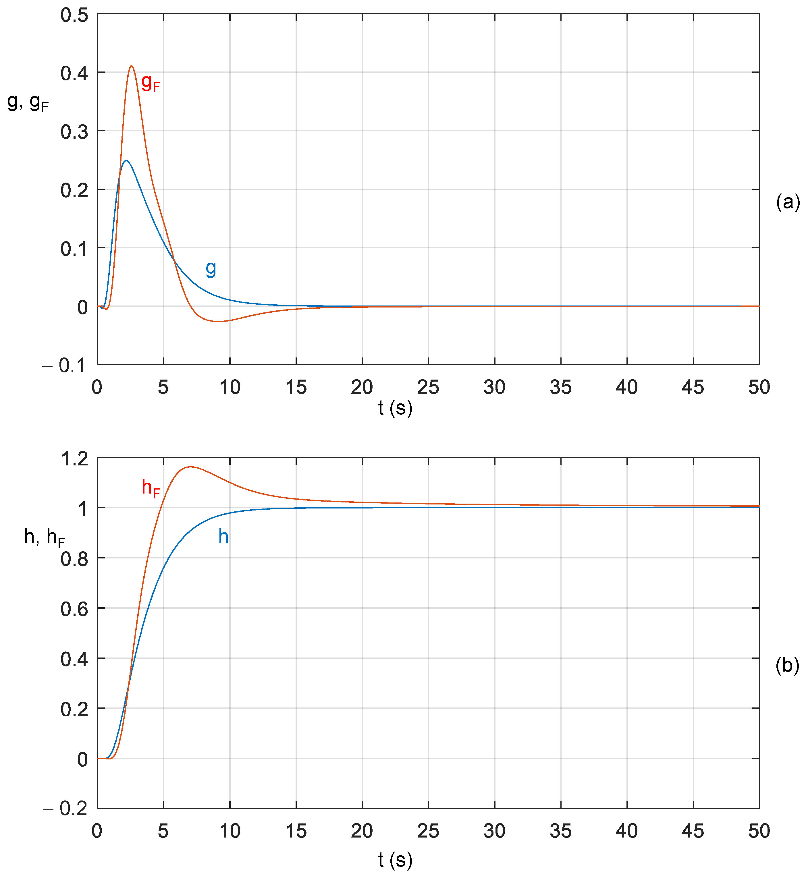
Figure 1 shows the plots of the corresponding impulse and step responses in MATLAB. For illustration, the responses of the IOS (α = 1) were added. Since the same results were obtained in Micro-Cap, they were not added in Figure 1.
It follows from the comparison of the IOS and FOS responses in Figure 1 that the FOS responses exhibit less damping due to the increase in the α parameter from 1 to 1.2. In [35], only the step response hF is published, and its exact comparison with the analysis results of Figure 1 cannot be performed with the lack of numerical data. Therefore, the correctness of the results from Figure 1 was verified with the FFT test.

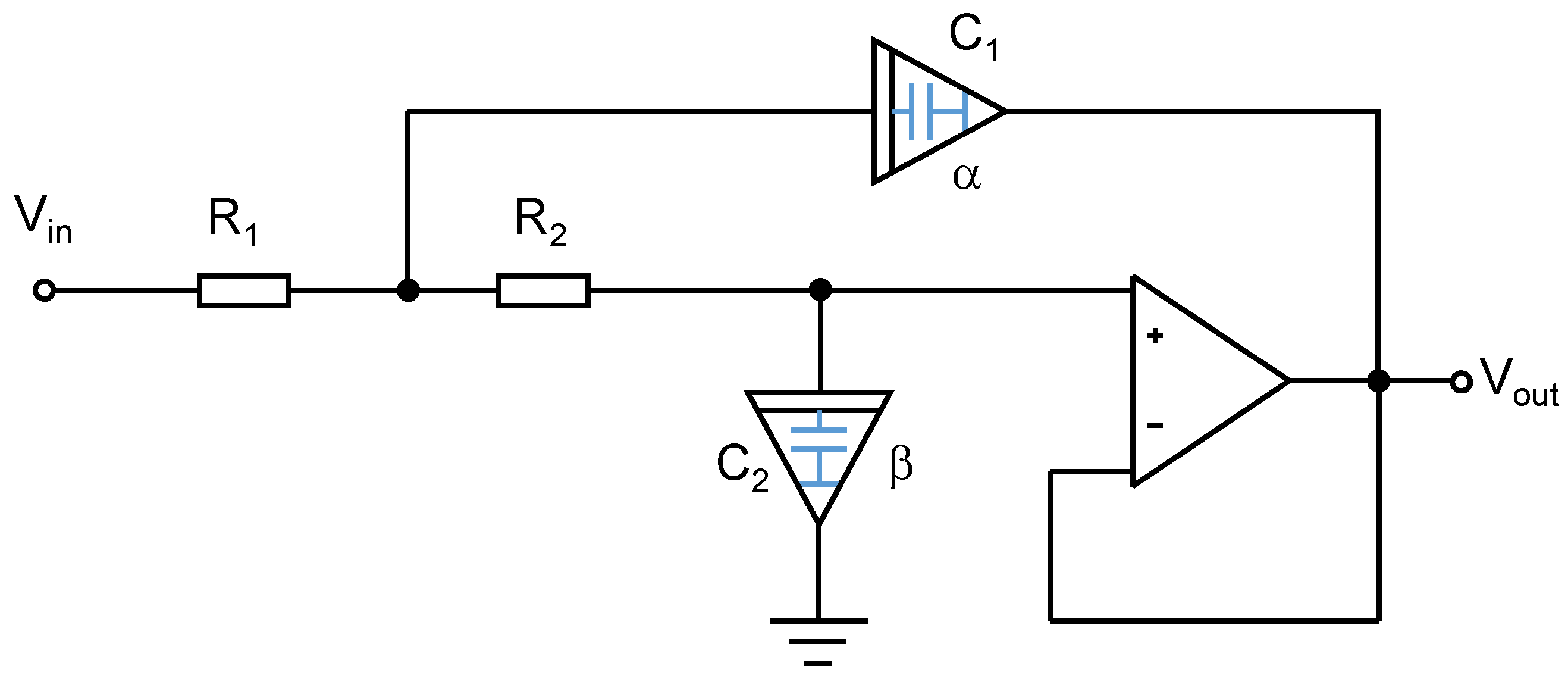
9.2. Commensurate Fractional-Order Sallen–Key Filter

Figure 2 shows a simplified version of the Sallen–Key filter from [35] with an operational amplifier as the voltage buffer. Instead of classical capacitors, fractors of the impedances 1/(sα C1) and 1/(sβ C2) are used, where α, β ∈ R+.
For α = β, the filter behaves like a commensurate FOS with the transfer function
K F ( s ) = ω 0 2 s 2 α + s α ω 0 Q + ω 0 2 ,
where the pseudo-natural frequency and pseudo-quality factor are given by
ω 0 = 1 R 1 R 2 C 1 C 2 , Q = R 1 R 2 R 1 + R 2 C 1 C 2 .
Transfer function (59) can be rewritten in the form
K F ( s ) = 1 s ω 0 F 2 α + 1 Q s ω 0 F α + 1 ,
where
ω 0 F = ω 0 1 / α
is the corner frequency of the asymptotic frequency characteristic of the fractional filter.
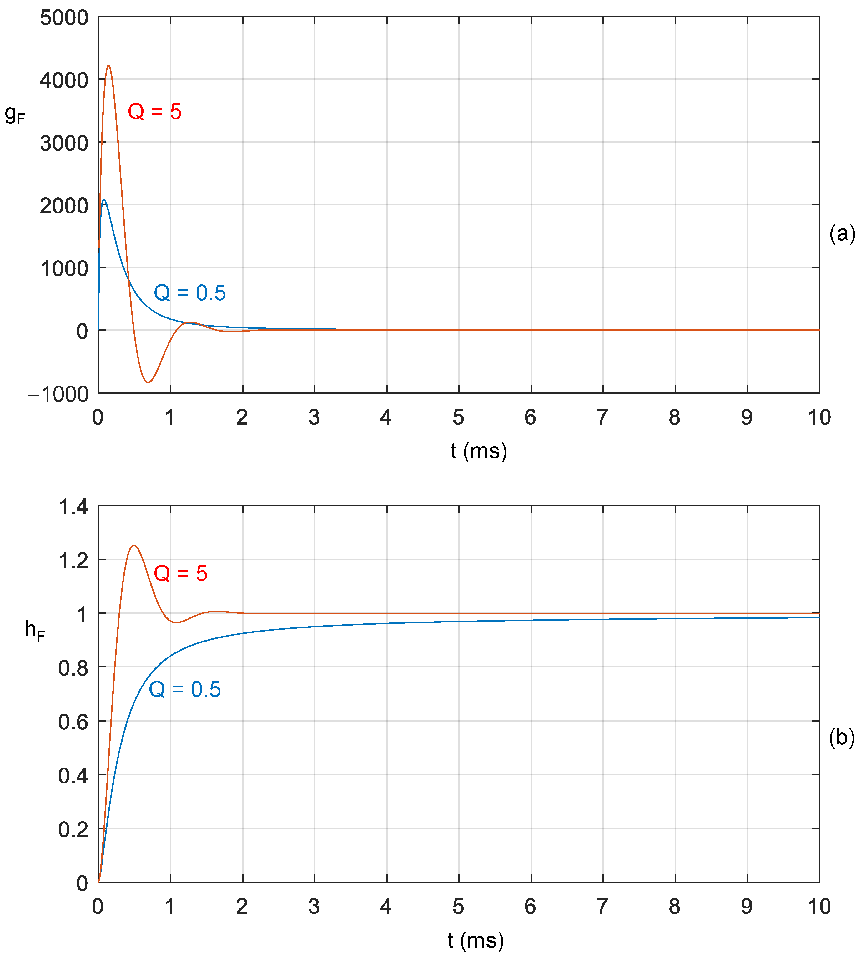
Consider the Sallen–Key filter with the following parameters:
α = 0.8, R1 = R2 = 91 kΩ, C1 = 100 nF/s1−α, C2 = 1 nF/s1−α.
It can be shown that Q = 5 and the corner frequency f0F = ω0F/(2π) is 1 kHz. Note that the natural frequency of the associated IOS, resulting from (60), is about 174 Hz.
First, the impulse response for the case α = 1 will be found. Transfer function (59) has a pair of complex conjugate poles
c = a ± ib, a = −109.2808, b = 1091.4412.
According to Table 3, the impulse response is
g ( t ) = k e a t sin ( b t ) ,
k = ω 0 1 1 4 Q 2 1098.3134 .
Hence the impulse and step responses of the fractional filter are
g F ( t ) = k Im ε 0 ( t , c ; α , α ) ,
h F ( t ) = k Im ε 0 ( t , c ; α , α + 1 ) .
If the parameters C1 and C2 in the filter are changed to have the values C1 = C2 = 10 nF, then the corner and natural frequencies are preserved, but the quality factor is reduced to 0.5. This will correspond to an integer-order filter with critical damping and the two-fold real pole −ω0. For critical damping, the impulse response has the form
g ( t ) = ω 0 2 t e ω 0 t .
The corresponding responses of the fractional filter are then as follows:
g F ( t ) = ω 0 2 ε 1 ( t , ω 0 ; α , α ) ,
h F ( t ) = ω 0 2 ε 1 ( t , ω 0 ; α , α + 1 ) .
The respective waveforms computed in MATLAB are shown in Figure 3.
The obtained plots of the impulse and step responses satisfy the check for the basic features (the limit values at times zero and infinity are correct, and the local maxima and minima of the step response correspond to the impulse response passages through zero). Looking at the step response for Q = 5, we find a much smaller overshoot than for classical second-order IOS. This observation is consistent with the well-known fact that lowering the order 2α below 2 (i.e., α = 0.8 < 1) acts as additional damping.
The filter in Figure 2 was also modeled in SPICE. Two different models were used:
Model 1: Modeling transfer function (61) using the Laplace voltage-controlled voltage source.
Model 2: Model of the circuit in Figure 2.
In Model 2, for a conclusive comparison with the MATLAB results, the OpAmp follower was modeled with a simple controlled source (gain = 1). The fractors were modeled with Laplace current-controlled voltage sources.
Regarding the Micro-Cap outputs, Models 1 and 2 show a perfect match with the MATLAB results.
However, the experiments revealed errors in the SPICE transient analysis if the fractional-order filter was set to an unstable mode due to an inappropriately chosen parameter α. In contrast, the method based on basis functions gives correct results.
The stability analysis of transfer function (59) or (61), respectively, leads to the observation that the fractional-order Sallen–Key filter in Figure 2 is stable for
α < 2 1 1 π tan 1 4 Q 2 1 .
For Q = 5, the threshold value of the parameter α is 1.0638.
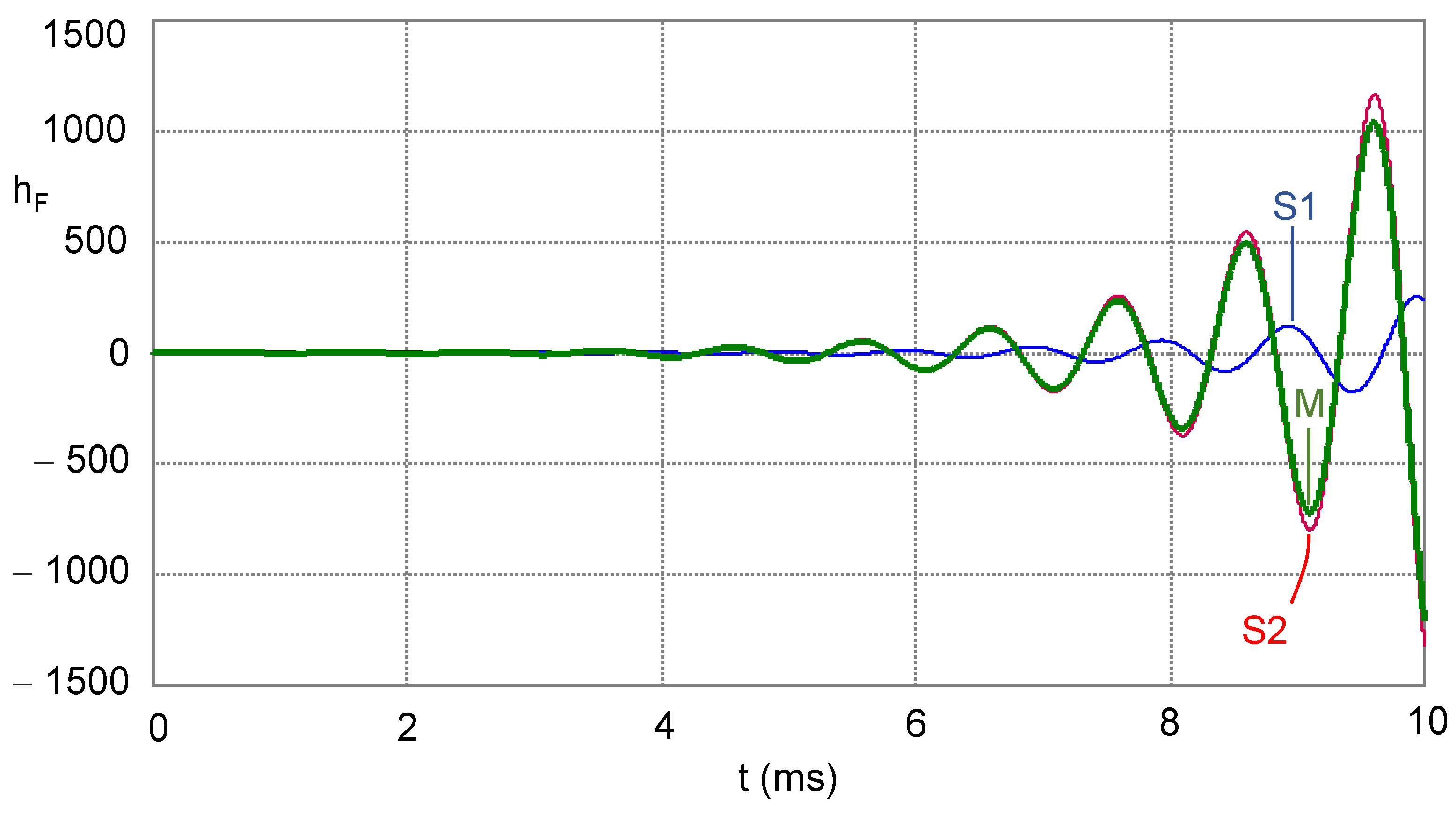
The filter was re-designed for α = 1.15, i.e., for the unstable mode. For Q = 5 and f0F = 1 kHz, it now comes out as
R1 = R2 = 91 kΩ, C1 = 4.71 nF/s1−α, C2 = 47.1 pF/s1−α.
Figure 4 shows the results of the simulation of the step response in Micro-Cap. The simulation was performed with default simulation parameters and with a step ceiling of 10 μs, which is one thousandth of the simulation time. For comparison, data from MATLAB were imported into the simulation program environment, showing the results obtained with the basis functions method.
Figure 4 shows that Micro-Cap calculates completely different responses for Models 1 and 2, which should be interchangeable. The response for Model 2 is close to the response computed from the basis functions in MATLAB. The FFT check cannot be used to verify the results because the system is unstable. However, by lowering the step ceiling 100-fold to 0.1 μs, the simulation program can be forced to perform a more accurate, but time-consuming, transient analysis. Then, the step response obtained using Method 2 is overlaid with the response computed using MATLAB.
The above pitfalls of the transient analysis of FOS in a SPICE simulation environment certainly deserve attention. The unpleasant fact is that different SPICE-family programs may deal with the same simulation task differently depending on the properties of their internal algorithms, and that the particular simulator chosen may evaluate the response differently depending on how the model of a fractional-order circuit is constructed. The cause should be sought in the specifics of the method of a convolutional transient analysis that SPICE uses to solve circuits with Laplace sources. Anyway, the method utilizing basis functions does not deal with such problems in principle.

10. Conclusions

The main results of this work are summarized in the following points:
  • The natural response of an arbitrary commensurate fractional-order system with transfer function (4) and parameter α can be expressed as a linear combination of the basis functions of time t, which are based on the two-parameter Mittag–Leffler functions Eα,β, β =α and their derivatives.
  • All the basis functions can be uniformly generated by using Podlubny’s function εk(t, c; α, α), where c is the corresponding sα-domain pole of the system, and k is its multiplicity.
  • There are unambiguous assignments between the generating functions as well as the individual basis functions of the integer-order system and the associated commensurate fractional-order system according to Table 5. This can be used to quickly construct an analytical formula for the impulse response of the fractional-order system if one knows the response formula of the classical integer-order system.
  • The step response of any commensurate fractional-order system with transfer function (4) can be written as a linear combination of basis functions whose generating function is εk(t, c; α, α + 1).
  • The transient analysis of FOSs via basis functions can lead to credible results also in cases when SPICE-family programs fail.

Author Contributions

Conceptualization, D.B. and V.B.; methodology, D.B.; software, Z.K. and Z.B.; validation, D.B., Z.K. and Z.B.; investigation, D.B.; writing—original draft preparation, D.B.; writing—review and editing, V.B.; visualization, V.B.; supervision, D.B.; project administration, V.B.; funding acquisition, Z.K. All authors have read and agreed to the published version of the manuscript.

Funding

This research was funded by the Czech Science Foundation, grant number: 20-26849S. It was also supported by the infrastructure of K206 and K217, University of Defence Brno, Czech Republic.

Data Availability Statement

Not applicable.

Conflicts of Interest

The authors declare no conflict of interest.

References

  1. Desoer, C.A.; Kuh, E.S. Basic Circuit Theory; McGraw-Hill Book Company: New York, NY, USA, 1969. [Google Scholar]
  2. Zadeh, L.A.; Desoer, C.A. Linear System Theory; The State Space Approach; McGraw-Hill Book Company: New York, NY, USA, 1963. [Google Scholar]
  3. Desoer, C.A. Modes in Linear Circuits. IRE Trans. Circuit Theory 1960, 7, 211–223. [Google Scholar] [CrossRef]
  4. Goldstein, H. Classical Mechanics; Addison-Wesley Publishing Co.: Reading, MA, USA, 1950. [Google Scholar]
  5. Gorenflo, R.; Kilbas, A.A.; Mainardi, F.; Rogosin, S. Mittag-Leffler Functions, Related Topics and Applications, 2nd ed.; Springer: Berlin/Heidelberg, Germany, 2020. [Google Scholar] [CrossRef]
  6. Acar, N.; Atici, F.M. Exponential functions of discrete fractional calculus. Appl. Anal. Discret. Math. 2013, 7, 343–353. [Google Scholar] [CrossRef]
  7. Lorenzo, C.F.; Hartley, T.T. Fractional Trigonometry and the Spiral Functions. Nonlinear Dynam. 2004, 38, 23–60. [Google Scholar] [CrossRef]
  8. Almusharrf, A. Development of Fractional Trigonometry and an Application of Fractional Calculus to Pharmacokinetic Model. Master’s Thesis, Western Kentucky University, Bowling Green, KY, USA, 2011. [Google Scholar]
  9. Yang, X.-J. Fractional Trigonometric Functions in Complex-valued Space: Applications of Complex Number to Local Fractional Calculus of Complex Function. arXiv 2011, arXiv:1106.2783v1. [Google Scholar] [CrossRef]
  10. Cerutti, R.A.; Luque, L.L. k-Fractional Trigonometric Functions. Int. J. Contemp. Math. Sci. 2014, 9, 569–578. [Google Scholar] [CrossRef]
  11. Mei, Z.D.; Peng, J.G.; Zhang, Y. Riemann-Liouville Fractional Cosine Functions. arXiv 2015, arXiv:1505.01388v1. [Google Scholar] [CrossRef]
  12. Chen, M.; Shao, S.; Shi, P. Robust Adaptive Control for Fractional-Order Systems with Disturbance and Saturation, 1st ed.; John Wiley & Sons Ltd.: Hoboken, NJ, USA, 2018. [Google Scholar]
  13. Podlubny, I. Fractional Differential Equations; Mathematics in Science and Engineering; Academic Press: Cambridge, MA, USA, 1999; Volume 198. [Google Scholar]
  14. Biolek, D.; Biolková, V.; Kolka, Z. Semi-Symbolic Transient Analysis of Analog Fractional-Order Systems. In Proceedings of the 18th International Conference on Synthesis, Modeling, Analysis and Simulation Methods and Applications to Circuit Design (SMACD 2022), Villasimius, Italy, 12–15 June 2022. [Google Scholar] [CrossRef]
  15. Monjoe, C.A.; Chen, Y.Q.; Vinagre, B.M.; Xue, D.; Feliu, V. Fractional-Order Systems and Controls; Springer: London, UK, 2010. [Google Scholar] [CrossRef]
  16. Agrawal, O.P.; Kumar, P. Comparison of Five Numerical Schemes for Fractional Differential Equations. In Advances in Fractional Calculus; Sabatier, J., Agrawal, O.P., Machado, J.A.T., Eds.; Springer: Dordrecht, The Netherlands, 2007. [Google Scholar] [CrossRef]
  17. El-Sayed, A.M.A.; El-Mesiry, A.E.M.; El-Saka, H.A.A. Numerical solution for multi-term fractional (arbitrary) orders differential equations. Comput. Appl. Math. 2004, 23, 33–54. [Google Scholar] [CrossRef] [Green Version]
  18. Trigeassou, J.C.; Maamri, N.; Sabatier, J.; Oustaloup, A. State variables and transients of fractional order differential systems. Comput. Math. Appl. 2021, 64, 3117–3140. [Google Scholar] [CrossRef] [Green Version]
  19. Wang, K.-J.; Sun, H.-C.; Fei, Z. The transient analysis for zero-input response of fractal RC circuit based on local fractional derivative. Alex. Eng. J. 2020, 59, 4669–4675. [Google Scholar] [CrossRef]
  20. Rani, D.; Mishra, V.; Cattani, C. Numerical Inverse Laplace Transform for Solving a Class of Fractional Differential Equations. Symmetry 2019, 11, 530. [Google Scholar] [CrossRef] [Green Version]
  21. Yüce, A.; Tan, N. On the approximate inverse Laplace transform of the transfer function with a single fractional order. Trans. Inst. Meas. Control 2020, 43, 1376–1384. [Google Scholar] [CrossRef]
  22. Brzeziński, D.W.; Ostalczyk, P. Numerical calculations accuracy comparison of the Inverse Laplace Transform algorithms for solutions of fractional order differential equations. Nonlinear Dynam. 2016, 84, 65–77. [Google Scholar] [CrossRef]
  23. Sheng, H.; Li, Y.; Chen, Y.Q. Application of numerical inverse Laplace transform algorithms in fractional calculus. J. Frankl. Inst. 2011, 348, 315–330. [Google Scholar] [CrossRef]
  24. Petráš, I. Stability of fractional-order systems with rational orders: A survey. Fract. Calc. Appl. Anal. 2009, 12, 269–298. [Google Scholar]
  25. Biolek, D.; Garrappa, R.; Biolková, V. Impulse response of commensurate fractional-order systems: Multiple complex poles. Fract. Calc. Appl. Anal. 2022, 25, 1837–1851. [Google Scholar] [CrossRef]
  26. Haubold, H.J.; Mathai, A.M.; Saxena, R.K. Mittag-Leffler Functions and their Applications. J. Appl. Math. 2011, 2011, 51. [Google Scholar] [CrossRef] [Green Version]
  27. Podlubny, I. Mittag-Leffler Function. MATLAB Central File Exchange. Available online: https://www.mathworks.com/matlabcentral/fileexchange/8738 (accessed on 10 July 2023).
  28. Xue, D. FOTF Toolbox. MATLAB Central File Exchange. Available online: https://www.mathworks.com/matlabcentral/fileexchange/60874 (accessed on 10 July 2023).
  29. Garrappa, R. The Mittag-Leffler Function. MATLAB Central File Exchange. Available online: https://www.mathworks.com/matlabcentral/fileexchange/48154 (accessed on 10 July 2023).
  30. Gorenflo, R.; Loutchko, J.; Luchko, Y. Computation of the Mittag-Leffler function and its derivatives. Fract. Calc. Appl. Anal. 2002, 5, 1–26. [Google Scholar]
  31. Garrappa, R.; Popolizio, M. Computing the Matrix Mittag-Leffler Function with Applications to Fractional Calculus. J. Sci. Comput. 2018, 77, 129–153. [Google Scholar] [CrossRef] [Green Version]
  32. Bateman, H.; Erdélyi, A. Tables of Integral Transforms; Bateman Manuscript Project; California Institute of Technology: Pasadena, CA, USA; McGraw-Hill Book Company, Inc.: New York, NY, USA, 1954. [Google Scholar]
  33. Garrappa, R. Numerical Evaluation of Two and Three Parameter Mittag-Leffler Functions. SIAM J. Numer. Anal. 2015, 53, 1350–1369. [Google Scholar] [CrossRef] [Green Version]
  34. Saxena, S.; Hote, Y.V.; Arya, P.P. Reduced-order modeling of commensurate fractional-order systems. In Proceedings of the 14th International Conference on Control, Automation, Robotics & Vision (ICARCV 2016), Phuket, Thailand, 13–15 November 2016. [Google Scholar] [CrossRef]
  35. Soltan, A.; Radwan, A.G.; Soliman, A.M. Fractional Order Sallen-Key and KHN Filters: Stability and Poles Allocation. Circuits Syst. Signal Process 2015, 34, 1461–1480. [Google Scholar] [CrossRef]
Figure 1. (a) Impulse responses gF and g, (b) step responses hF and h of the commensurate system with transfer function (55) and associated IOS with α = 1.
Algorithms 16 00335 g001
Figure 2. Fractional-order Sallen–Key filter (adopted from [35]).
Algorithms 16 00335 g002
Figure 3. (a) Impulse responses gF, (b) step responses hF of the commensurate Sallen–Key filter with transfer function (59) for α = 0.8 and for two different values of damping.
Algorithms 16 00335 g003
Figure 4. Simulated step responses hF of the commensurate Sallen–Key filter with transfer function (59) for α = 1.15 and Q = 5 (unstable mode); S1 (SPICE-Micro-Cap, Method 1), S2 (SPICE-Micro-Cap, Method 2), M (MATLAB, basis functions).
Algorithms 16 00335 g004
Table 1. Overview of the types of complex Mittag–Leffler functions (MLF) of the complex argument z and their relationships with each other and with exponential and gamma functions.
e z E α ( z ) E α , β ( z ) E α , β ( m ) ( z ) E α , β χ ( z ) E α , β χ ( m ) ( z )
e z e z E 1 ( z ) E 1 , 1 ( z ) E 1 , 1 ( m ) ( z ) E 1 , 1 1 ( z ) E 1 , 1 1 ( m ) ( z )
E α ( z ) k = 0 z k Γ α k + 1 E α , 1 ( z ) E α , 1 ( 0 ) ( z ) E α , 1 1 ( z ) E α , 1 1 ( 0 ) ( z )
E α , β ( z ) k = 0 z k Γ α k + β E α , β ( 0 ) ( z ) E α , β 1 ( z ) E α , β 1 ( 0 ) ( z )
E α , β ( m ) ( z ) k = 0 ( k + m ) ! k ! z k Γ α k + α m + β m ! E α , α m + β m + 1 ( z ) E α , β 1 ( m ) ( z )
E α , β χ ( z ) k = 0 ( χ ) k k ! z k Γ α k + β E α , β χ ( 0 ) ( z )
E α , β χ ( m ) ( z ) χ m E α , m α + β χ + m ( z ) k = 0 ( χ ) k + m k ! z k Γ α k + α m + β
Eα (z)—MLF with one parameter, α ∈ C, Re(α) > 0; Eα,β (z)—MLF with two parameters, α ∈ C, β ∈ C, Re(α) > 0, Re(β) > 0; E α , β ( m ) ( z ) m-th derivative of Eα,β(z) with respect to z, m ∈ N0, α ∈ C, β ∈ C, Re(α) > 0, Re(β) > 0; E α , β χ ( z ) —generalized MLF with three parameters, α ∈ C, β ∈ C, γ ∈ C, Re(α) > 0, Re(β) > 0, Re(γ) > 0; E α , β χ ( m ) ( z ) m-th derivative of E α , β χ ( z ) with respect to z, m ∈ N0, α ∈ C, β ∈ C, Re(α) > 0, Re(β) > 0; (χ)k = Γ (χ + k)/ Γ (χ) is the Pochhammer symbol.
Table 2. Basic relations between the time and Laplace domains for single and multiple real pole a.
s δ s α a k t α k δ 1 ( k 1 ) ! E α , α δ ( k 1 ) ( a t α )
integer order (α = 1)fractional order
Laplace domaintime domainLaplace domaintime domain
δ = 0 1 s a e a t 1 s α a t α 1 E α , α ( a t α )
1 s a k t k 1 ( k 1 ) ! e a t 1 s α a k t α ( k 1 ) ( k 1 ) ! t α 1 E α , α ( k 1 ) ( a t α )
Table 3. Basic relations between the time and Laplace domains for a simple pair of complex conjugate poles c = a + ib, c* = a − ib.
s δ ( s α a ) 2 + b 2 t α δ 1 b Im E α , α δ c t α
integer order (α = 1)fractional order
Laplace domain time domainLaplace domain time domain
δ = 0 b s a 2 + b 2 e a t sin ( b t ) b s α a 2 + b 2 t α 1 Im E α , α ( c t α )
b s 2 + b 2 sin ( b t ) b s 2 α + b 2 t α 1 Im E α , α ( i b t α ) = t α 1 sin α , α ( b t α )
δ = α s s a 2 + b 2 e a t [ a b sin ( b t ) + cos ( b t ) ] s α s α a 2 + b 2 t α 1 Im c b E α , α ( c t α ) = t α 1 a b Im E α , α ( c t α ) + Re E α , α ( c t α )
s s 2 + b 2 cos ( b t ) s α s 2 α + b 2 t α 1 Re E α , α ( i b t α ) = t α 1 cos α , α ( b t α )
s a s a 2 + b 2 e a t cos ( b t ) s α a s α a 2 + b 2 t α 1 Re E α , α ( c t α )
Table 4. Basic relations between the time and Laplace domains for a multiple pair of complex conjugate poles c = a + ib, c* = a − ib.
s δ [ ( s α a ) 2 + b 2 ] k t α 1 i = 0 k 1 2 ( 1 ) i + 1 A 2 i + 1 t 2 i α δ ( 2 i ) ! Im E α , α δ ( 2 i ) ( c t α ) + t α 1 i = 0 k 2 1 ( 1 ) i + 1 A 2 ( i + 1 ) t ( 2 i + 1 ) α δ ( 2 i + 1 ) ! Re E α , α δ ( 2 i + 1 ) ( c t α )
integer order (α = 1)fractional order
Laplace domain time domainLaplace domaintime domain
δ = 0 1 s a 2 + b 2 k e a t [ i = 0 k 1 2 ( 1 ) i + 1 ( 2 i ) ! A 2 i + 1 t 2 i sin ( b t ) + + i = 0 k 2 1 ( 1 ) i + 1 ( 2 i + 1 ) ! A 2 ( i + 1 ) t 2 i + 1 cos ( b t ) ] 1 s α a 2 + b 2 k t α 1 [ i = 0 k 1 2 ( 1 ) i + 1 ( 2 i ) ! A 2 i + 1 t 2 i α Im E α , α ( 2 i ) ( c t α ) + + i = 0 k 2 1 ( 1 ) i + 1 ( 2 i + 1 ) ! A 2 ( i + 1 ) t ( 2 i + 1 ) α Re E α , α ( 2 i + 1 ) ( c t α ) ]
1 s 2 + b 2 k i = 0 k 1 2 ( 1 ) i + 1 ( 2 i ) ! A 2 i + 1 t 2 i sin ( b t ) + + i = 0 k 2 1 ( 1 ) i + 1 ( 2 i + 1 ) ! A 2 ( i + 1 ) t 2 i + 1 cos ( b t ) 1 s 2 α + b 2 k t α 1 [ i = 0 k 1 2 ( 1 ) i + 1 ( 2 i ) ! A 2 i + 1 t 2 i α sin α , α ( 2 i ) ( b t α ) + + i = 0 k 2 1 ( 1 ) i + 1 ( 2 i + 1 ) ! A 2 ( i + 1 ) t ( 2 i + 1 ) α cos α , α ( 2 i + 1 ) ( b t α ) ]
δ = α s s a 2 + b 2 k e a t { i = 0 k 1 2 ( 1 ) i + 1 ( 2 i ) ! A 2 i + 1 [ 2 i t 2 i 1 sin ( b t ) + + t 2 i a sin ( b t ) + b cos ( b t ) ] + + i = 0 k 2 1 ( 1 ) i + 1 ( 2 i + 1 ) ! A 2 ( i + 1 ) [ ( 2 i + 1 ) t 2 i cos ( b t ) + + t 2 i + 1 a cos ( b t ) b sin ( b t ) ] } s α s α a 2 + b 2 k t α 1 { i = 0 k 1 2 ( 1 ) i + 1 ( 2 i ) ! A 2 i + 1 [ 2 i t ( 2 i 1 ) α Im E α , α ( 2 i 1 ) ( c t α ) + + t 2 i α a Im E α , α ( 2 i ) ( c t α ) + b Re E α , α ( 2 i ) ( c t α ) ] + + i = 0 k 2 1 ( 1 ) i + 1 ( 2 i + 1 ) ! A 2 ( i + 1 ) [ ( 2 i + 1 ) t 2 i α Re E α , α ( 2 i ) ( c t α ) + + t ( 2 i + 1 ) α a Re E α , α ( 2 i + 1 ) ( c t α ) b Im E α , α ( 2 i + 1 ) ( c t α ) ] }
s s 2 + b 2 k i = 0 k 1 2 ( 1 ) i + 1 ( 2 i ) ! A 2 i + 1 [ 2 i t 2 i 1 sin ( b t ) + t 2 i b cos ( b t ) ] + + i = 0 k 2 1 ( 1 ) i + 1 ( 2 i + 1 ) ! A 2 ( i + 1 ) [ ( 2 i + 1 ) t 2 i cos ( b t ) t 2 i + 1 b sin ( b t ) ] s α s 2 α + b 2 k t α 1 { i = 0 k 1 2 ( 1 ) i + 1 ( 2 i ) ! A 2 i + 1 [ 2 i t ( 2 i 1 ) α sin α , α ( 2 i 1 ) ( b t ) + t 2 i α b cos α , α ( 2 i ) ( b t ) ] + + i = 0 k 2 1 ( 1 ) i + 1 ( 2 i + 1 ) ! A 2 ( i + 1 ) [ ( 2 i + 1 ) t 2 i α cos α , α ( 2 i ) ( b t ) t ( 2 i + 1 ) α b sin α , α ( 2 i + 1 ) ( b t ) ] }
Table 5. Correspondence between the basis functions of IOS and FOS for various types of poles.
PolesInteger Order (α = 1)Fractional Order
Basis Functions
exp, sin, cos, tk
Generated from
f ( t ) = t k e c t
Basis Functions
MLF, sin, cos, ẽ, tαk, tα−1
Generated from
f F ( t ) = ε k ( t , c ; α , α )
simple real a e a t t 0 e a t e ˜ α , α ( a , t ) = t α 1 E α , α a t α ε 0 ( t , a ; α , α )
simple complex pair
c = a + ib, c* = a − ib
e a t sin ( b t )
e a t cos ( b t )
Im ( t 0 e c t )
Re ( t 0 e c t )
Im e ˜ α , α ( c , t )
Re e ˜ α , α ( c , t )
Im ε 0 ( t , c ; α , α )
Re ε 0 ( t , c ; α , α )
simple imaginary pair
c = +ib, c* = −ib
sin ( b t )
cos ( b t )
Im ( t 0 e j b t )
Re ( t 0 e j b t )
Im e ˜ α , α ( i b , t ) = si n ˜ α , α ( b , t )
Re e ˜ α , α ( i b , t ) = co s ˜ α , α ( b , t )
Im ε 0 ( t , i b ; α , α )
Re ε 0 ( t , i b ; α , α )
multiple real a t k e a t t k e a t t α k t α 1 E α , α ( k ) a t α ε k ( t , a ; α , α )
multiple complex pair
c = a + ib, c* = a − ib
t k e a t sin ( b t )
t k e a t cos ( b t )
Im ( t k e c t )
Re ( t k e c t )
t α k Im t α 1 E α , α ( k ) ( c t α )
t α k Re t α 1 E α , α ( k ) ( c t α )
Im ε k ( t , c ; α , α )
Re ε k ( t , c ; α , α )
multiple imaginary pair
c = +ib, c* = −ib
t k sin ( b t )
t k cos ( b t )
Im ( t k e i b t )
Re ( t k e i b t )
t α k t α 1 sin α , α ( k ) ( b t α )
t α k t α 1 cos α , α ( k ) ( b t α )
Im ε k ( t , i b ; α , α )
Re ε k ( t , i b ; α , α )
Table 6. Parameters of the partial fraction expansion of transfer function (55).
kakbkPkrPki
1−22.4369 0.0244
2−4.8430 0.9733
3−2.7791 −9.9797
4−2.1809 10.0304
5−1.0017 −3.1207
6−0.4993 1.5711
7−18.80142.1491−0.0086−0.0386
8−18.8014−2.1491−0.00860.0386
9−1.82821.73670.25920.7145
10−1.8282−1.73670.2592−0.7145
Disclaimer/Publisher’s Note: The statements, opinions and data contained in all publications are solely those of the individual author(s) and contributor(s) and not of MDPI and/or the editor(s). MDPI and/or the editor(s) disclaim responsibility for any injury to people or property resulting from any ideas, methods, instructions or products referred to in the content.

