Abstract
Classifying digital images using neural networks is one of the most fundamental tasks within the field of artificial intelligence. For a long time, convolutional neural networks have proven to be the most efficient solution for processing visual data, such as classification, detection, or segmentation. The efficient operation of convolutional neural networks requires the use of data augmentation and a high number of feature maps to embed object transformations. Especially for large datasets, this approach is not very efficient. In 2017, Geoffrey Hinton and his research team introduced the theory of capsule networks. Capsule networks offer a solution to the problems of convolutional neural networks. In this approach, sufficient efficiency can be achieved without large-scale data augmentation. However, the training time for Hinton’s capsule network is much longer than for convolutional neural networks. We have examined the capsule networks and propose a modification in the routing mechanism to speed up the algorithm. This could reduce the training time of capsule networks by almost half in some cases. Moreover, our solution achieves performance improvements in the field of image classification.
1. Introduction
For processing visual data, convolutional neural networks (CNNs) are proving to be the best solutions nowadays. The most popular applications of convolutional neural networks in the field of image processing are image classification [1,2], object detection [3,4], semantic segmentation [5,6] and instance segmentation [7,8]. However, the biggest challenge of convolutional neural networks is their inability to recognize pose, texture and deformations of an object, caused by the pooling layers. Pooling layers are used in the feature maps. Where we can find several types of this layer: max pooling, min pooling, average pooling and sum pooling are the most common types of pooling layers [9]. Due to this layer, the efficiency of the convolutional neural network to recognize the same object in different input images under different conditions is high. At the same time, the size of the tensors is reduced due to the pooling layer, thus reducing the computational complexity of the network. In most cases, pooling layers are one of the best tools for feature extraction; however, they introduce spatial invariance in convolutional neural networks. Due to the nature of the pooling layer, a great amount of information is lost, which in some cases may even be important features in the image. To compensate for this, the convolutional neural network needs a substantial amount of training data where data augmentation is necessary.
Geoffrey Hinton and his research team introduced capsule network theory as an alternative to convolutional neural networks. Hinton et al. published the first paper in the field of capsule networks in 2011 [10], where the potential of the new theory is explained, but the solution for effective training it is not yet available. The next important milestone came in 2017, when Sabour et al. introduced the dynamic routing algorithm between capsule layers [11]. Thanks to this dynamic routing algorithm, the training and optimization of capsule-based networks can be performed efficiently. Finally, Hinton et al. published a matrix capsule-based approach in 2018 [12]. These are the three most important results that the inventors of the theory have published in the field of capsule networks. The basic building block of convolutional neural networks is the neuron, while capsule networks are made up of so-called capsules. A capsule is a group of related neurons, where each neuron’s output represents a different property of the same feature. Hence, the input and output of the capsule networks are both vectors (n-dimensional capsules), while the neural network works with scalar values (neurons). Instead of pooling layers, a dynamic routing algorithm was introduced in capsule networks. In this approach, the lower-level features (lower-level capsules) will only be sent to higher-level capsules that match its contents. This property makes capsule networks a more effective solution than convolutional neural networks in some use cases.
However, the training process for capsule networks can be much longer than for convolutional neural networks, where due to the high number of parameters, the memory requirements of the network can be much higher. Therefore, for complex datasets (e.g., large input images, high number of output classes), presently, capsule networks do not perform well yet. This is due to the complexity of the dynamic routing algorithm. For this reason, we have attempted to make modifications to the dynamic routing algorithm. Our primary aim was to reduce the time of the training process, and secondly to achieve a higher efficiency. In our method, we reduced the weight of the input capsule vector during the optimization in the routing process. We also proposed a parameterizable activation function interpreted in terms of vectors, based on the squash function. In this paper, we demonstrate the effectiveness of our proposed modified routing algorithm and compare it with other capsule network-based methods and convolutional neural network-based approaches.
This paper is structured as follows. In Section 2, we provide the theoretical background of the capsule network theory proposed by Hinton et al. [10] and Sabour et al. [11]. Section 3 clarifies our improved routing mechanism for capsule network and our parameterizable activation squash function. Section 4 describes the capsule network architecture used in this research. In Section 5, we present the datasets used to compare the dynamic routing algorithm and our proposed solution. Our results are summarized in Section 6, where we compare our improved routing solution with Sabour et al.’s method, and with some recently published neural network-based solutions. Finally, our conclusions based on our results are summarized in Section 7.
2. Theory of Capsule Network
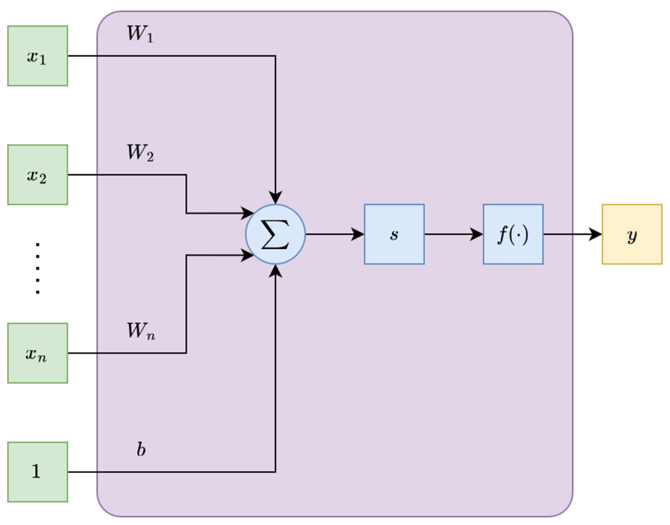
The capsule network [10,11,12] (or CapsNet) is very similar to the classical neural network. The main difference is the basic building block. In the neural network, we use neurons, but in the capsule network, we can find capsules. Figure 1 and Figure 2 show the main differences between the classical artificial neurons and the capsules.
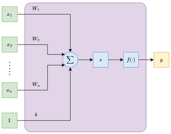
Figure 1.
Typical structure of a neuron. (green: inputs, blue: operations, yellow: output, purple: neuron).

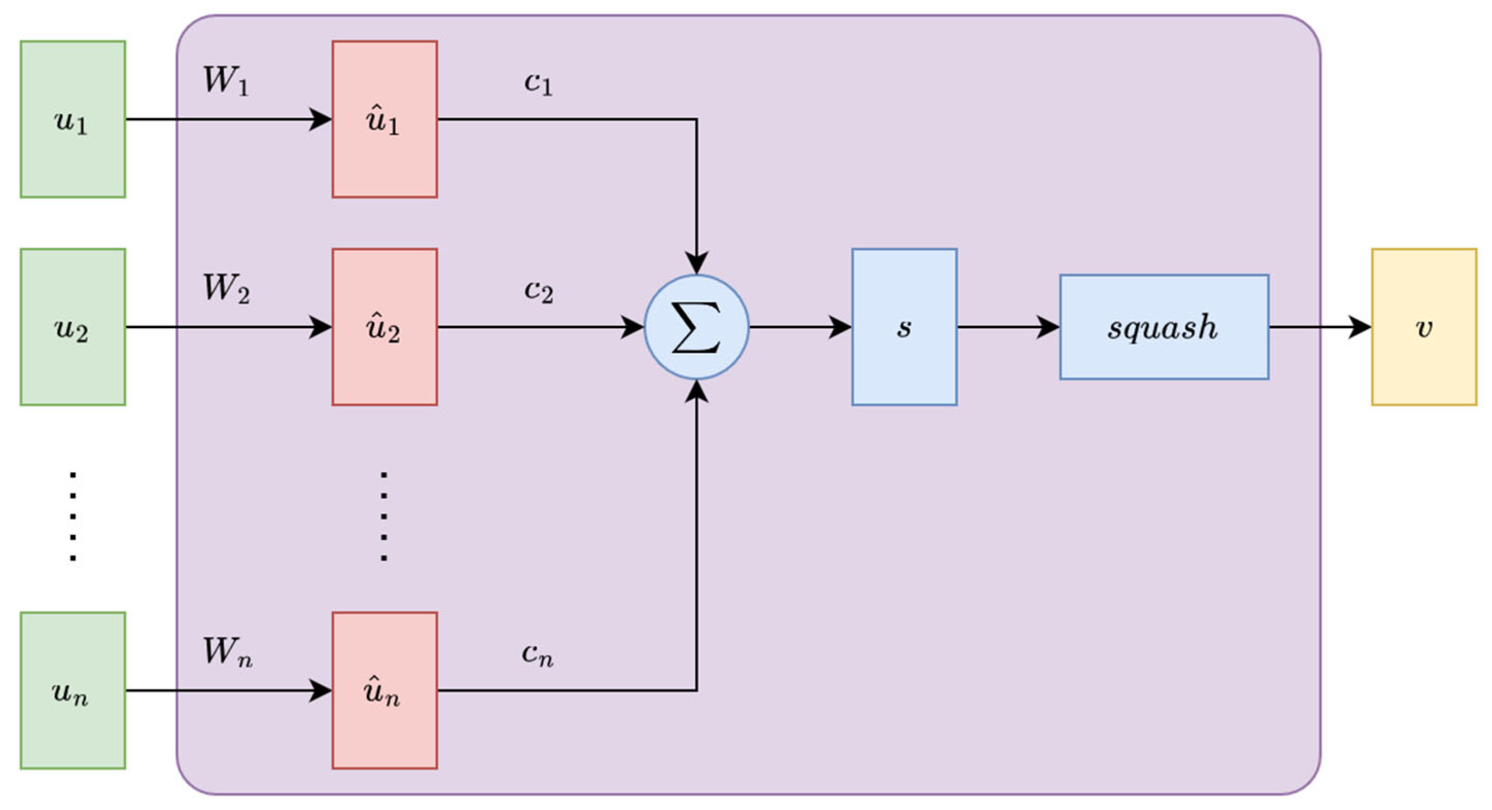
Figure 2.
Typical structure of a capsule. (green: inputs, red: prediction vectors, blue: operations, yellow: output, purple: capsule).
A capsule is a group of neurons that perform a multitude of internal computation and encapsulate the results of the computations into an n-dimensional vector. This vector is the output of the capsule. The length of this output vector is the probability and the direction of the vector, indicating certain properties about the entity.
In a capsule-based network, we use routing-by-agreement, where the output vector of any capsule is sent to all higher-level capsules. Each capsule output is compared with the actual output of the higher-level capsules. Where the outputs match, the coupling coefficient between the two capsules are increased.
Let be a lower-level capsule and be a higher-level capsule. The prediction vector is calculated as follows:
where is a trainable weighting matrix and is an output pose vector from the -th capsule to the -th capsule. The coupling coefficients are calculated with a simple SoftMax function, as follows:
where is the log probability of capsule coupled with capsule , and it is initialized with zero values. The total input to capsule is a weighted sum over the prediction vectors, calculated as follows:
In capsule networks, we use the length of the output vector to represent the probability for the capsule. Therefore, we use a non-linear activation function, which is called the squashing function. The squashing function is the next:
We can use the dynamic routing algorithm (by Sabour et al. [11]) to update the values in every iteration. In this case, the goal is to optimize the vector. In the dynamic routing algorithm, the vector is updated in every iteration, as follows:
3. Improved Routing Algorithm
Our experiments on capsule network theory have shown that the input tensor in the dynamic routing algorithm has too large an impact on the output tensor and greatly increaes the processing time. When calculating the output vector , the formula includes the input twice:
To improve the routing mechanism between lower-level and higher-level capsules, the following modifications to the routing algorithm are proposed:
Let
where is the value of the -th neuron of the -th capsule. If is an intermediate capsule layer, then is the number of output capsules. If is an output capsule layer, then is the number of possible object categories.
Let
where , let
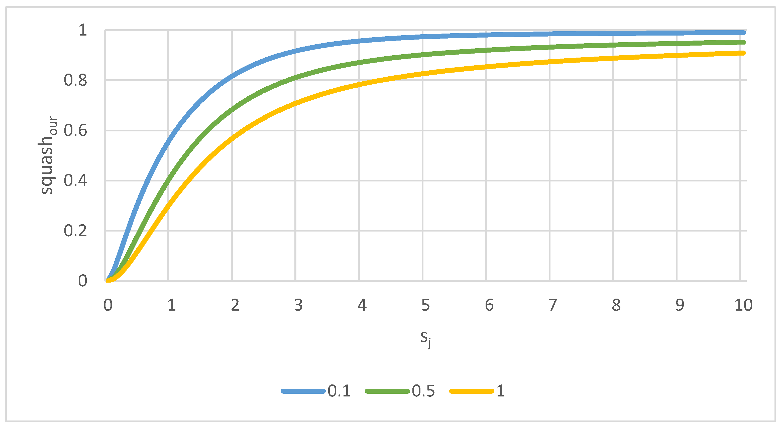
This minimal modification makes the routing algorithm simpler and faster to compute. Our other proposed change concerns the squashing function. In the last capsule layer, we use a modified squashing function, as follows:
where is a fine-tuning parameter. Based on our experience, we used in this work. Figure 3 shows a simple example of our squash function in a one-dimensional case for different values of .

Figure 3.
Our squash activation function with different values.
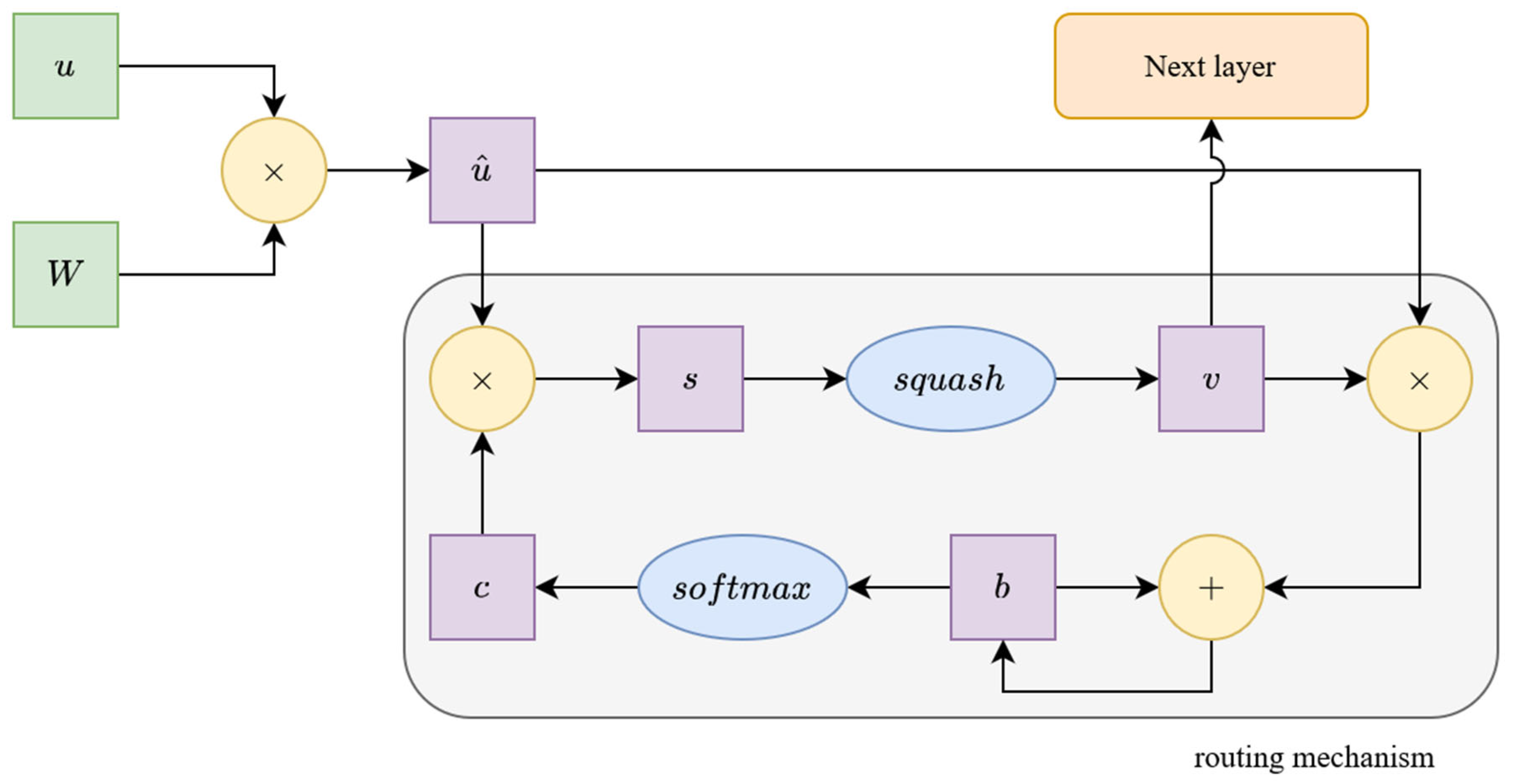
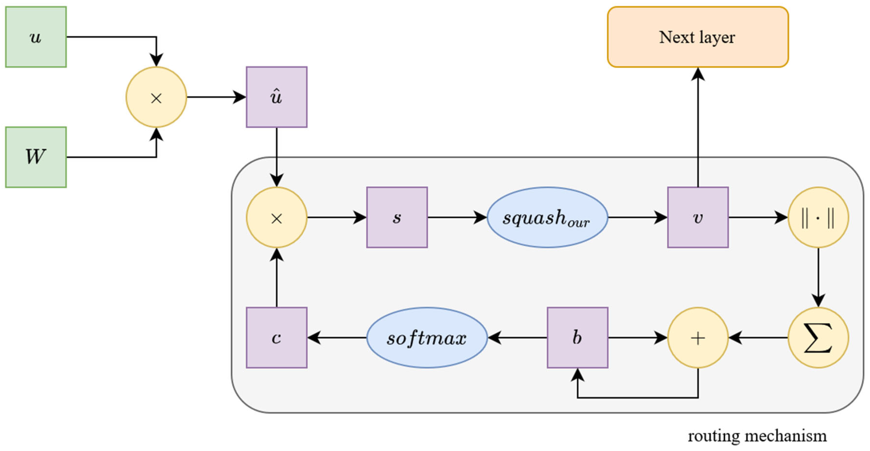
Figure 4 and Figure 5 show a block diagram of the dynamic routing algorithm and our improved routing solution, where the main differences between the two methods are clearly visible.
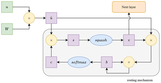
Figure 4.
Block diagram of the dynamic routing algorithm by Sabour et al. [11]. (green: inputs, yellow: operations, blue: activations, purple: internal tensors).

Figure 5.
Block diagram of our proposed routing algorithm. (green: inputs, yellow: operations, blue: activations, purple: internal tensors).
4. Network Architecture
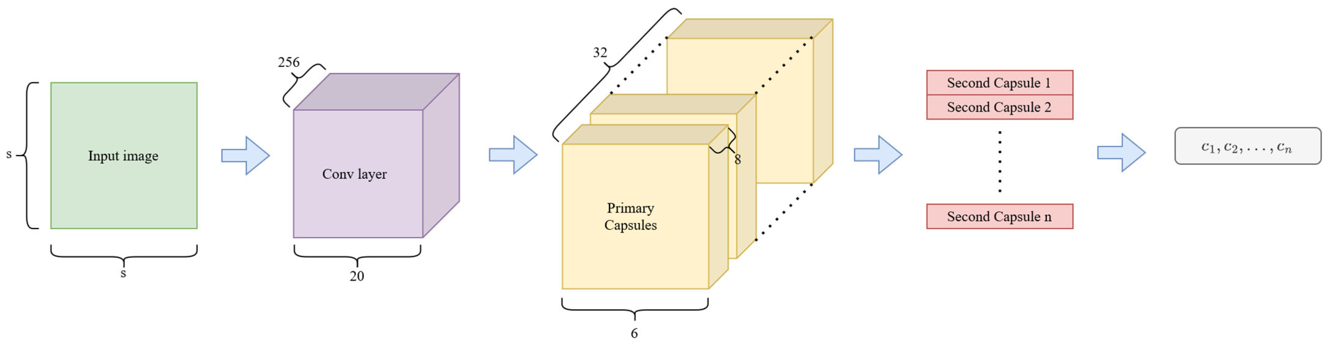
In this work, we have used the network architecture proposed by Sabour et al. [11] to compare our proposed routing mechanism with other optimization solutions in the field of capsule networks. This capsule network architecture is shown in Figure 6. The original paper used a fixed -sized input tensor, because they only tested the network efficiency for the MNIST [13] dataset. In contrast, we trained and tested the capsule networks for six fundamentally different datasets in the field of image classification. In our work, the shape of the input layer varies depending on the dataset. We used the following input shapes: , and . After the input layer, the capsule network architecture consisted of three main components: the first is a convolutional layer, the next is the primary capsule layer, and the last one is the secondary capsule layer.
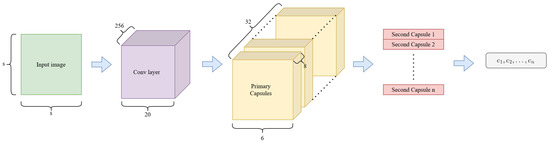
Figure 6.
The capsule network architecture used in the research, based on work by Sabour et al. [11]. (green: input, purple: convolutional layer, yellow: primary capsule layer, red: secondary capsule layer, gray: prediction).
The convolution layer contains convolution kernels of size with a stride of , and a ReLU (rectified linear unit) [14] activation layer. This convolutional layer generates the main visual features based on intensities for the primary capsule layer.
The primary capsule block contains a convolutional layer, where both the input and the output are of the size . This capsule block also contains a squash layer. In this case, the original squash function (Equation (4)) is used for both implementations. The output of this block contains capsules, where each capsule has dimensions. This capsule block contains advanced features, which are passed onto the secondary capsule block.
The secondary capsule block has one capsule per class. As mentioned earlier, we worked with several different datasets, so the number of capsules in this capsule block varied, always according to the class number of the dataset: , or . This capsule block contains the routing mechanism, which is responsible for determining the connection weights between the lower and higher capsules. Therefore, this capsule block represents the main difference between the solution of Sabour et al. and our presented method. In this block, we applied our proposed squash function (Equation (11)). The secondary capsule block contains a trainable matrix, called (Equation (14)). The shape of the matrix, for both solutions, is , where is the number of output classes and depends on the input image shape as follows:
where is the size of the input image. The routing algorithm was run through iterations in both cases. The output of this capsule block is a -dimensional vector per each class. This means that the block produces -dimensional capsules, where is the number of output classes. The length of the output capsules represents the probability values belonging to the given class.
5. Datasets
In this work, different datasets were used. A classification task was performed for each dataset in our work. The datasets needed to have different levels of complexity. This allowed us to test as wide a range of datasets as possible. The selected datasets include grayscale and color images. The number of classes also varies, from to . The size of the images is typically small, but here, again, we tried to experiment with different sizes. The datasets included a fixed background which had been used, as well as a variable color background which had been applied. Table 1 shows the main properties of the datasets that we used in this research.

Table 1.
Main properties of the datasets used.
5.1. MNIST
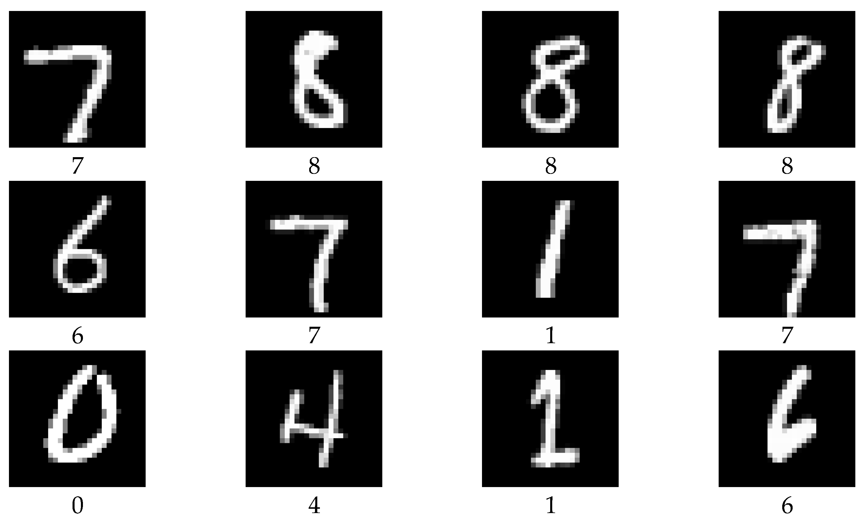
The MNIST dataset (Modified National Institute of Standards and Technology dataset) is a large set of handwritten digits (from to ) that is one of the most widely used datasets in the field of image classification. The MNIST dataset contains training images and testing images, where every image is grayscale with a pixel width and pixel height. Figure 7 shows some samples from this dataset.

Figure 7.
Sample data from MNIST dataset.
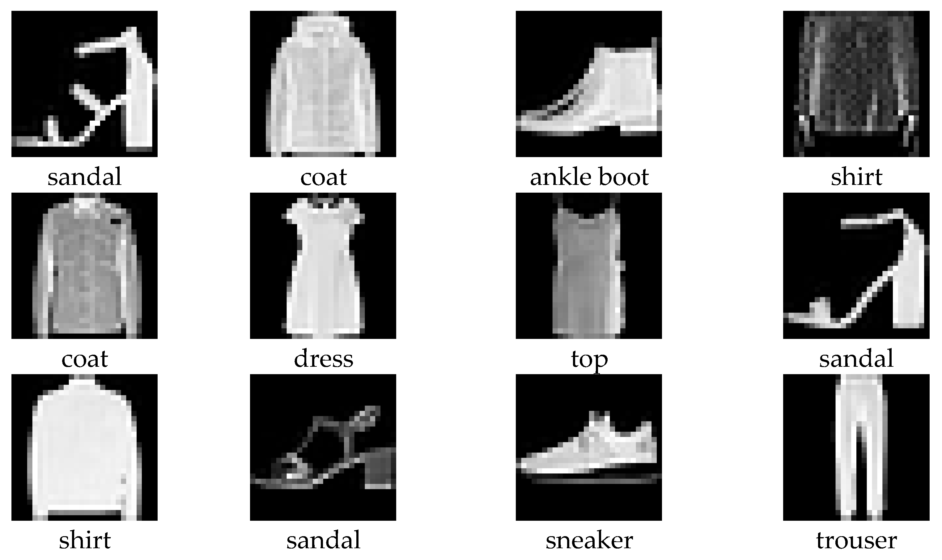
5.2. Fashion-MNIST
The Fashion-MNIST (or F-MNIST) dataset is very similar to the MNIST dataset. The main parameters are the same. It contains training and testing examples. Every sample is pixels in width and pixels in height, and a grayscale image where colors are inverted (an intensity value of represents the darkest color). The Fashion-MINST dataset contains fashion categories: t-shirt/top, trouser, pullover, dress, coat, sandal, shirt, sneaker, bag and ankle boot. Figure 8 shows some samples from this dataset.

Figure 8.
Sample data from Fashion-MNIST dataset.
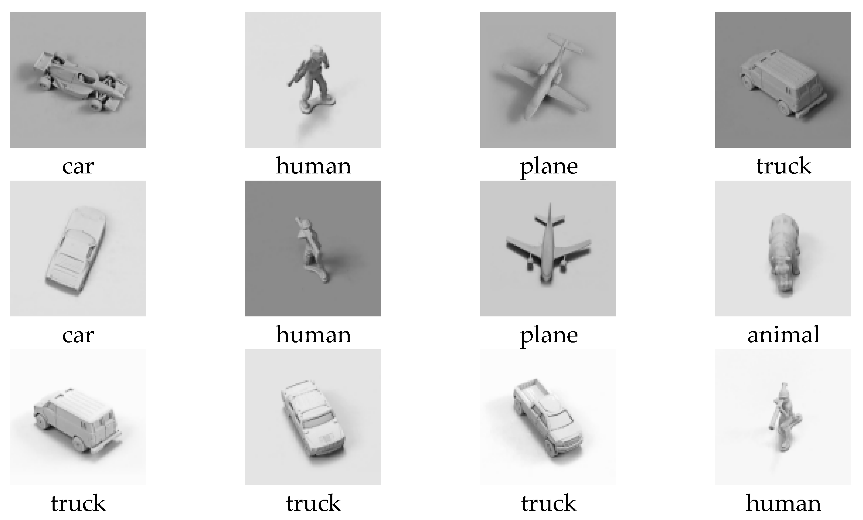
5.3. SmallNORB
The SmallNORB dataset contains images of 3D objects. The specialty of this dataset is that the images were taken under several different lighting conditions and poses. This dataset contains images of toys belonging different categories: four-legged animals, human figures, airplanes, trucks and cars. The images were taken with two cameras under lighting conditions, elevations and azimuths. All images are grayscale, with a size of pixels in width by pixels in height. However, in this work, we resized the images to pixels. Figure 9 shows some samples from this dataset.
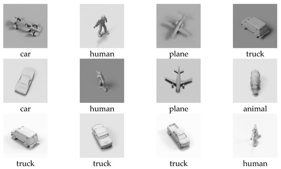
Figure 9.
Sample data from SmallNORB dataset.
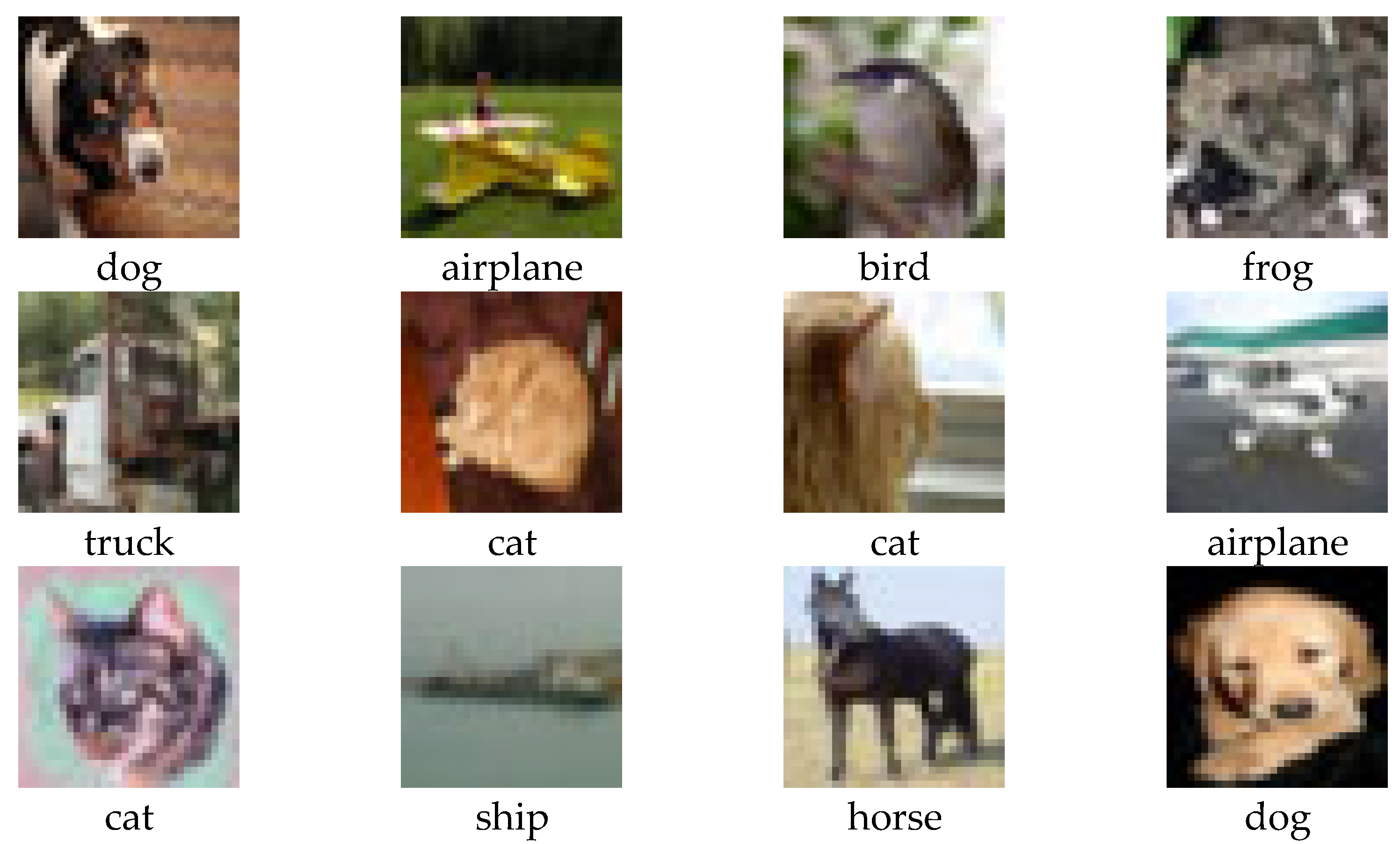
5.4. CIFAR10
The CIFAR10 (Canadian Institute for Advanced Research) dataset is one of the most widely used datasets in the field of machine learning-based image classification. This dataset is composed of RGB colored images, where images are the training samples and images are the testing samples. Each image is pixels wide and pixels high. The object categories are the following: airplanes, cars, birds, cats, deer, dogs, frogs, horses, ships and trucks. Figure 10 shows some samples from this dataset.
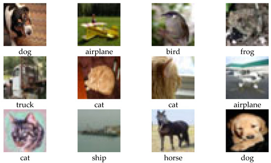
Figure 10.
Sample data from CIFAR10 dataset.
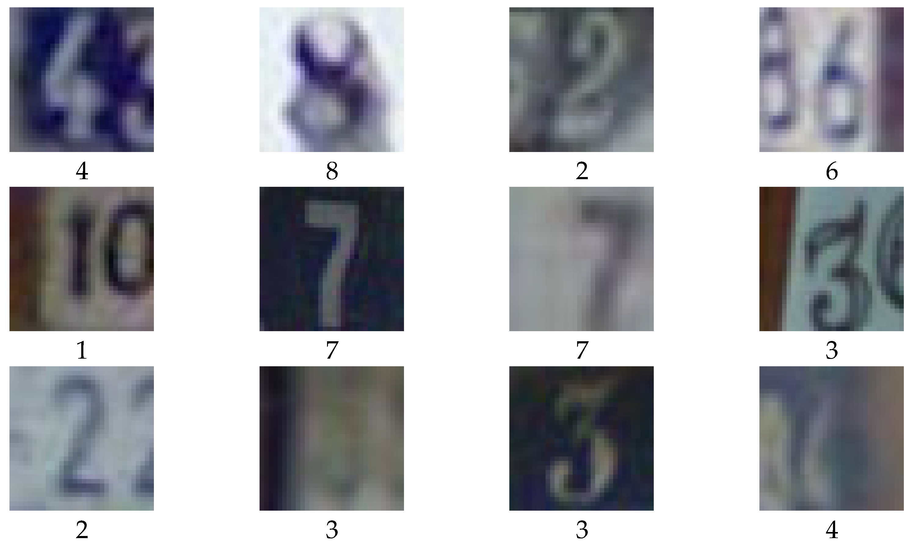
5.5. SVHN
The SVHN (Street View House Numbers) dataset contains small, cropped digits, like the MNIST dataset. However, the SVHN dataset is slightly more complex than the MNIST dataset. The SVHN is obtained from house numbers in Google Street View, where the background of the digits is not homogeneous and images may also include part of the adjacent digit. This property makes the SVHN dataset more difficult to classify than the MNIST dataset. The size of the images in this dataset is pixels wide and pixels high. The SVHN dataset contains training samples and testing samples. Figure 11 shows some samples from this dataset.
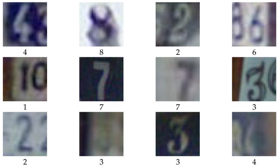
Figure 11.
Sample data from SVHN dataset.
5.6. GTSRB
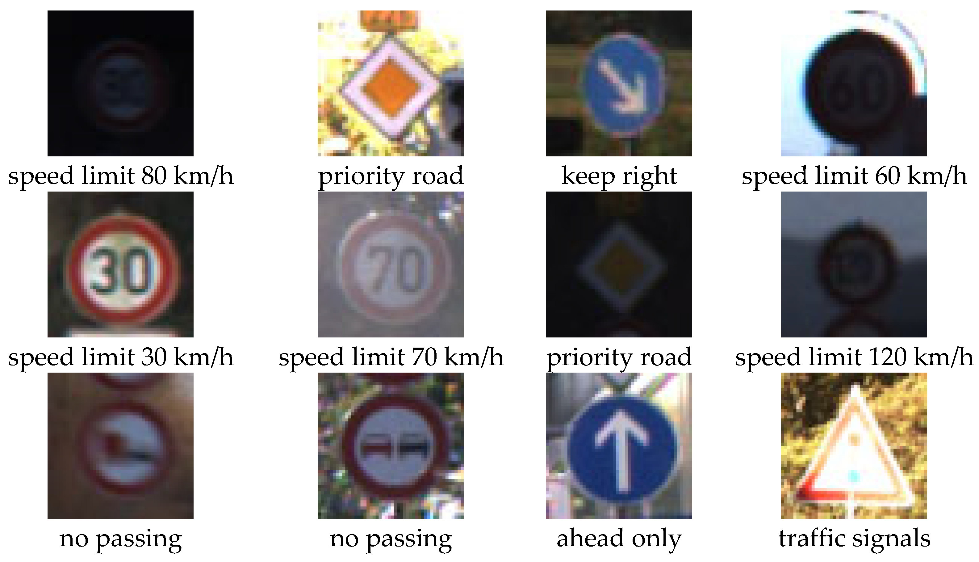
The GTSRB (German Traffic Sign Recognition Benchmark) dataset includes classes of traffic signs. Each image contains one traffic sign with varying light conditions and rich backgrounds. Images are pixels wide and pixels high. The traffic sign classes are the following: speed limit {, , , , , , , } km/h, end of speed limit (80 km/h), no passing, no passing for vehicles over 3.5 metric tons, right-of-way at the next intersection, priority road, yield, stop, no vehicles, vehicles over 3.5 metric tons prohibited, no entry, general caution, dangerous curve to the {left, right}, double curve, bumpy road, slippery road, road narrows on the right, road work, traffic signals, pedestrians, children crossing, bicycles crossing, beware of ice/snow, wild animals crossing, end of all speed and passing limits, turn {right, left} ahead, ahead only, go straight or {right, left}, keep {right, left}, roundabout mandatory, end of no passing and end of no passing by vehicles over 3.5 metric tons. Figure 12 shows some samples from this dataset.

Figure 12.
Sample data from GTSRB dataset.
6. Results
In this work, the network architecture presented in Section 4 has been designed in three different ways and trained separately on the datasets presented in Section 5. The difference between the three networks is the routing algorithm used: the first is the original capsule network by Sabour et al., the second is our modified capsule network with some improvements, and the third is the efficient vector routing by Heinsen [20]. Capsule networks are trained separately on the presented dataset. For the implementation, we used Python 3.9.16 [21] programming language with PyTorch 1.12.1 [22] machine learning framework and CUDA toolkit 11.6 platform. The capsule networks are trained on the Paperspace [23] online artificial intelligence platform with an Nvidia Quadro RTX4000 series graphical processing unit.
We trained all networks for epochs with the Adam [24] optimizer algorithm where the train and test batch size are both . We also attempted to train the networks over many more epochs, but found that the difference between the three solutions does not change significantly after epochs. In this study, we used initial learning rate. In each epoch, we reduced the learning rate as follows:
where is the initial learning rate and is the learning rate in the -th epoch. We used and hyperparameter values to control the exponential decay, and to prevent any division by zero in the implementation. In the training process, we used the same loss function as proposed by Sabour et al.
where
, and are hyperparameters. In the present work, we used the same values for these hyperparameters as proposed by Sabour et al., in this case, , and . The original study also used reconstruction in the training process; however, we did not apply this in our work. During training without reconstruction, the efficiency of the capsule network is reduced. In the long term, we want to translate our results in the field of capsule networks into real-world applications. In this respect, reconstruction of the input image is a rarely necessary step. Therefore, we explicitly investigated the ability of capsule networks without reconstruction.
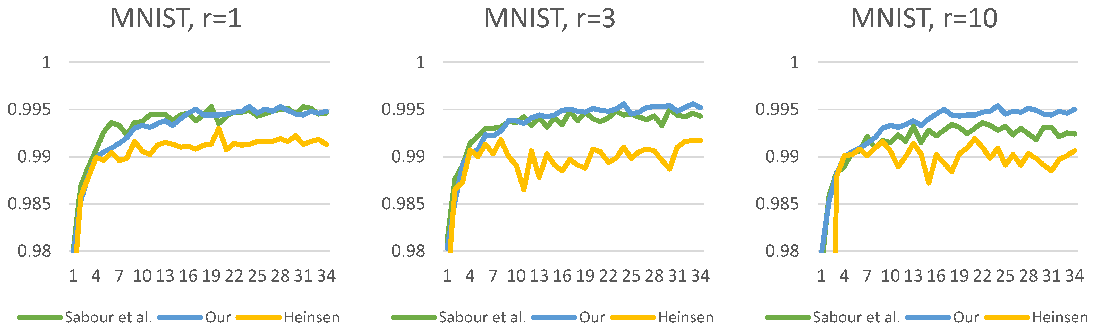
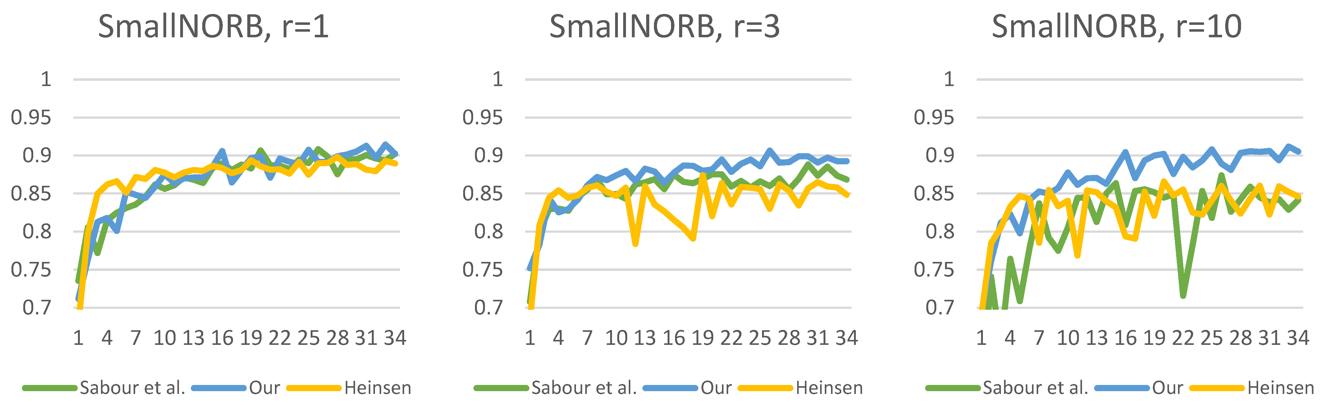
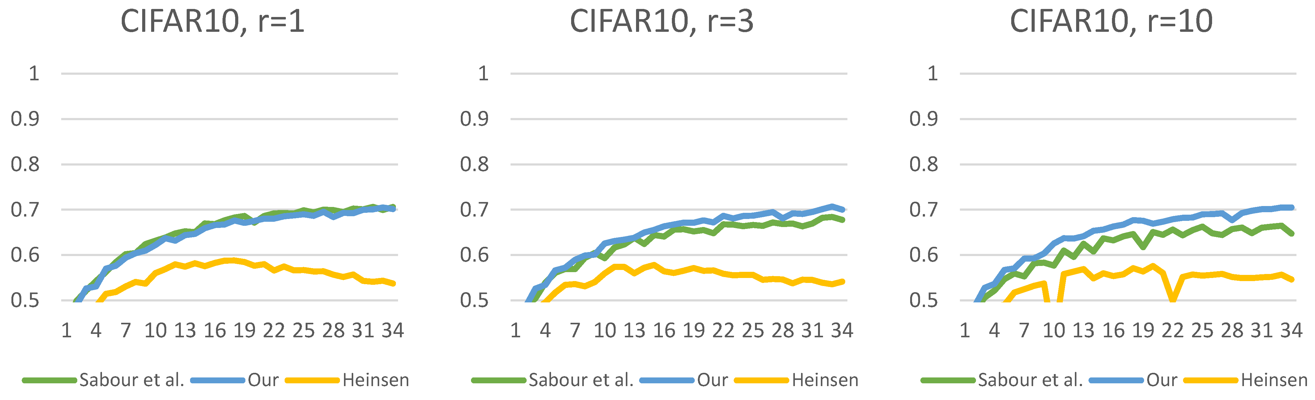
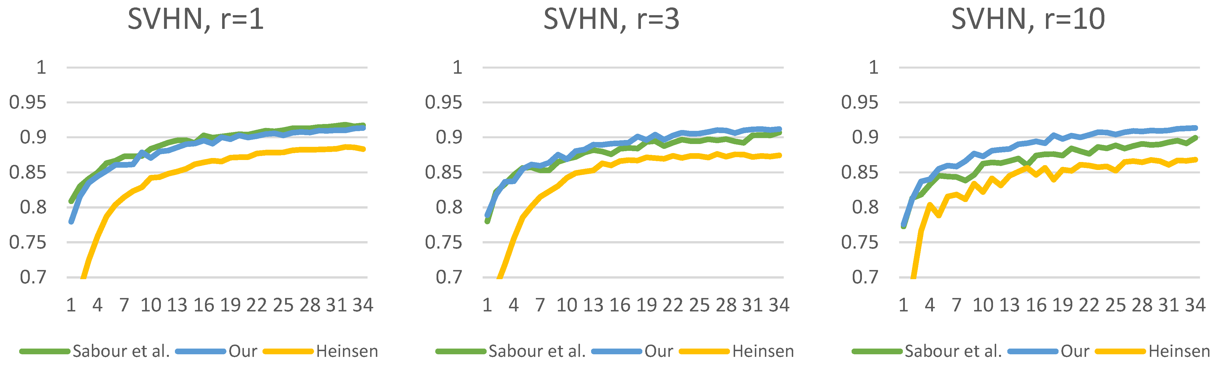
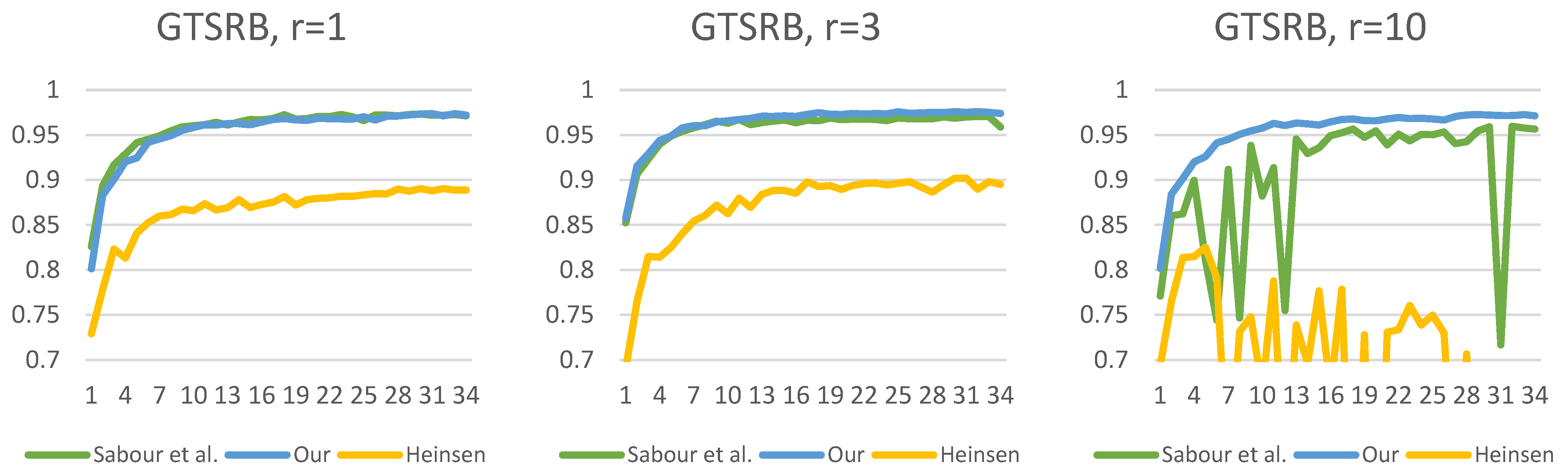
Figure 13, Figure 14, Figure 15, Figure 16, Figure 17 and Figure 18 show the accuracy of the training processes for the test sets of the presented datasets with different numbers of routings. The value of indicates the number of iterations which the routing algorithm has optimized the coefficients. Based on Sabour et al.’s experiment, the is a good choice; however, we showed the efficiency with and . This makes the difference more visible between the routing methods. As can be seen, for all datasets, we have achieved efficiency gains compared to the two other capsule network solutions. The difference in efficiency between our and Sabour et al.’s solutions is minimal for about the first epochs; however, after that, there is a noticeable difference in the learning curve. Although Heinsen’s solution also proves to be effective in most cases; its performance is slightly lower than the other two solutions. It is also noticeable that changing the number of iterations has a much larger impact on Sabour et al.’s solution and that of Heinsen. Our proposed solution is less sensitive to the iteration value chosen during the optimization.
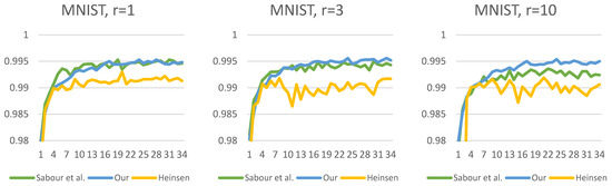
Figure 13.
Classification test accuracy on MNIST dataset.
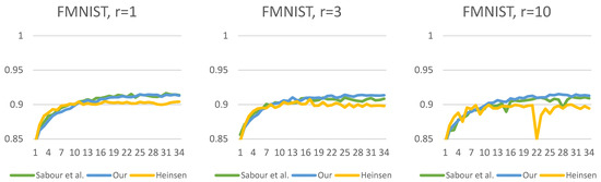
Figure 14.
Classification test accuracy on Fashion-MNIST dataset.
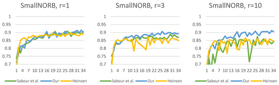
Figure 15.
Classification test accuracy on SmallNORB dataset.
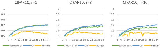
Figure 16.
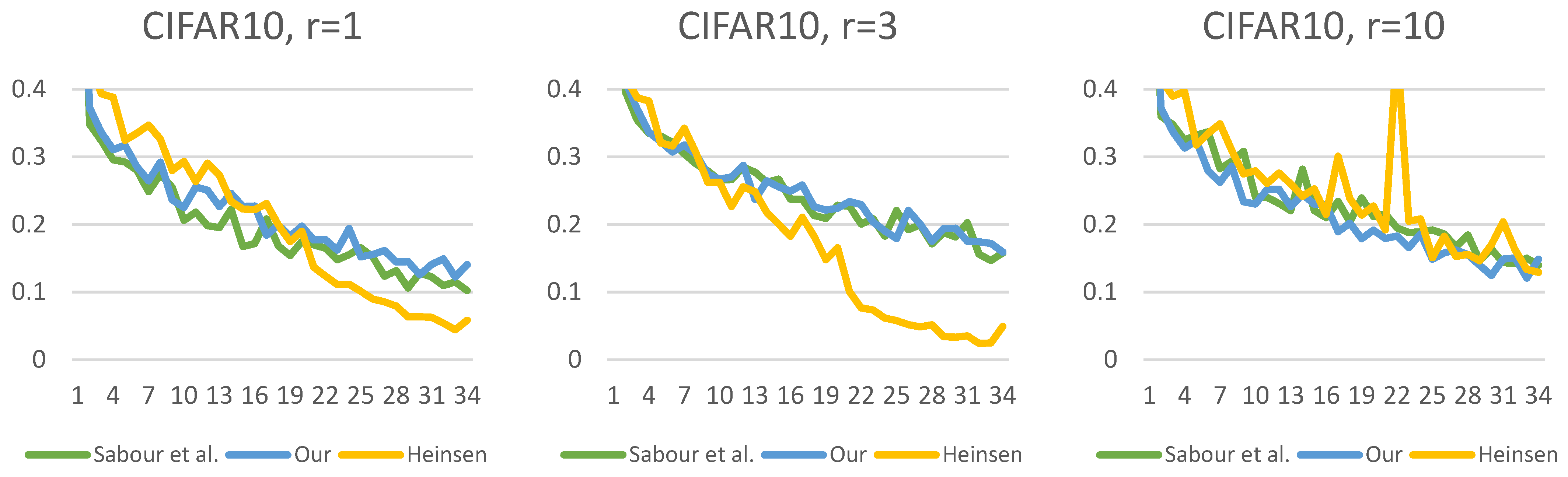
Classification test accuracy on CIFAR10 dataset.

Figure 17.
Classification test accuracy on SVHN dataset.
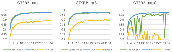
Figure 18.
Classification test accuracy on GTSRB dataset.
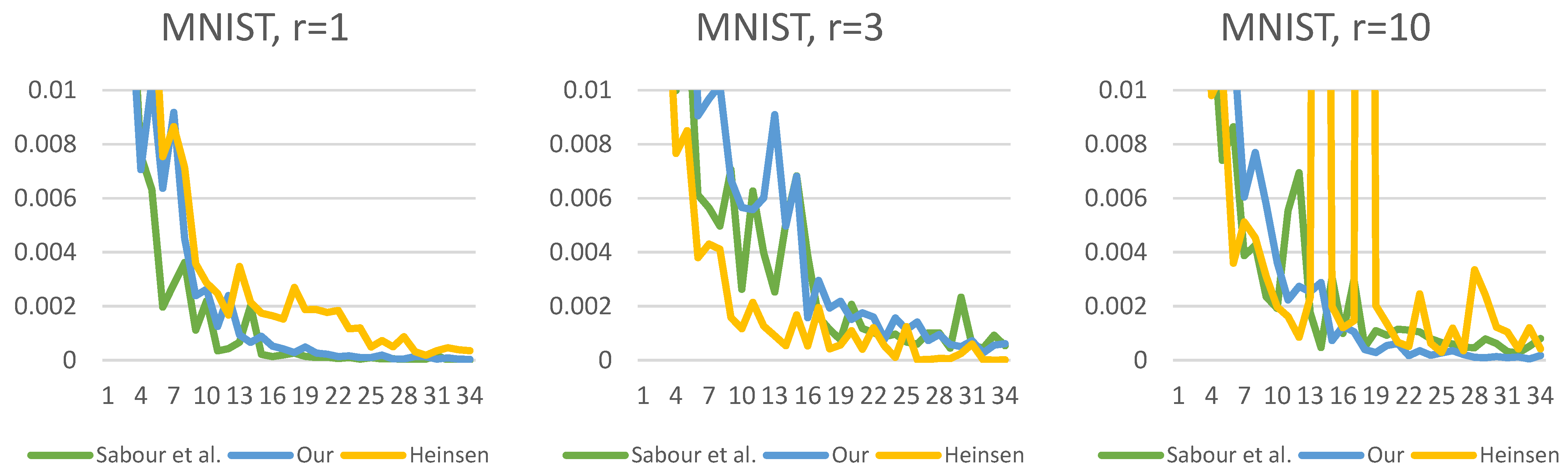
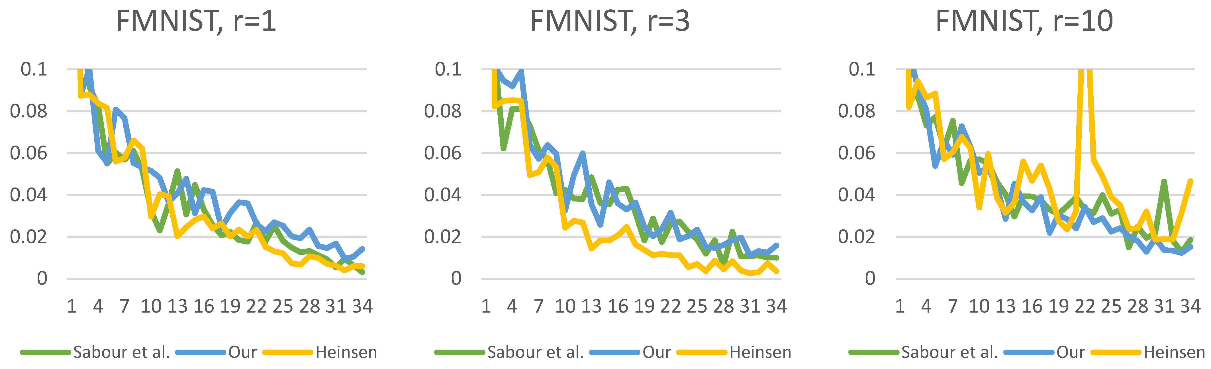
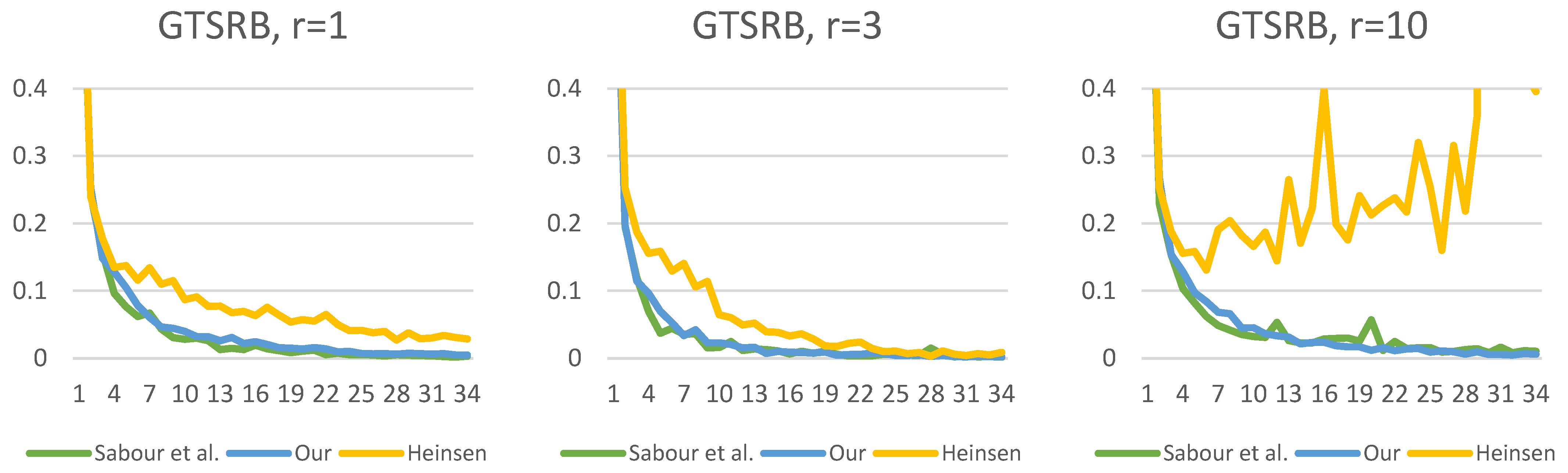
Figure 19, Figure 20, Figure 21, Figure 22, Figure 23 and Figure 24 show the test losses (Equation (14)) during the training processes with different numbers of routings. There is not much difference in the loss function, but it is noticeable that our solution is less noisy and converges more smoothly.

Figure 19.
Classification test loss on MNIST dataset.
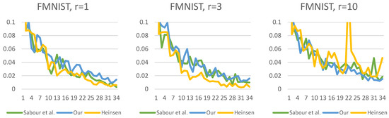
Figure 20.
Classification test loss on Fashion-MNIST dataset.
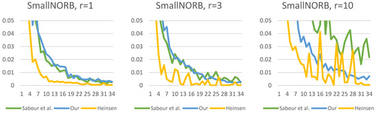
Figure 21.
Classification test loss on SmallNORB dataset.
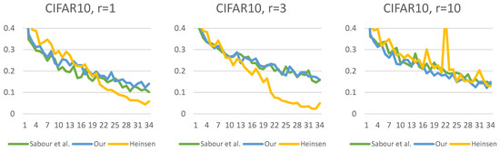
Figure 22.
Classification test loss on CIFAR10 dataset.
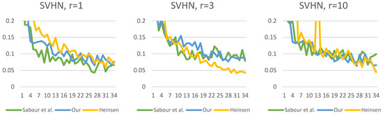
Figure 23.
Classification test loss on SVHN dataset.

Figure 24.
Classification test loss on GTSRB dataset.
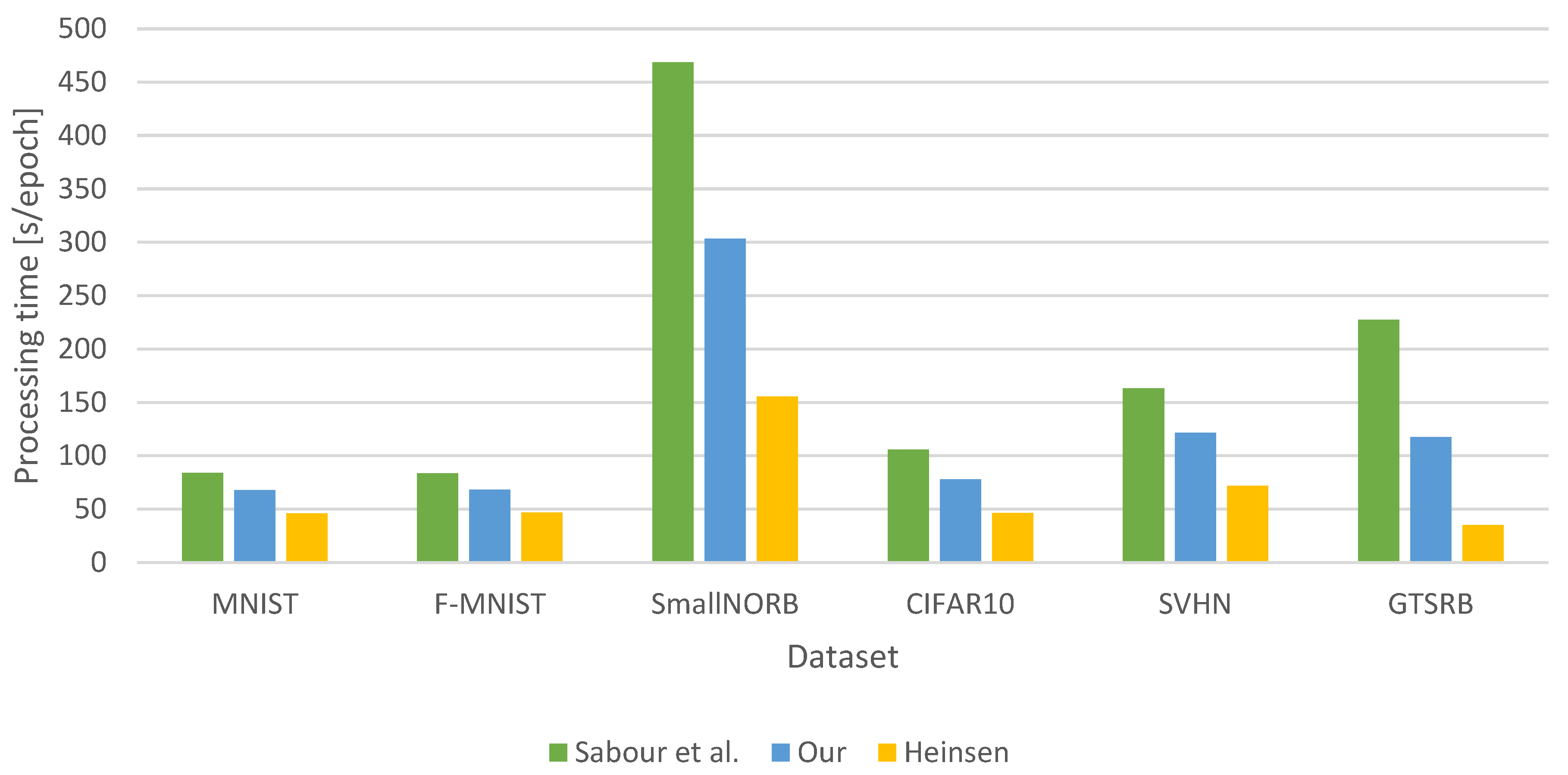
Figure 25 shows the processing times for the three capsule-based networks. It can be seen that for all datasets, the capsule network was faster with our proposed routing algorithm than with the dynamic routing algorithm introduced by Sabour et al. The smallest increase was achieved for the Fashion-MNIST and MNIST datasets, but this still represents an and a speedup. For more complex datasets, much higher speed increases were achieved. A running time reduction of 25.55% was achieved for SVHN and 26.54% for CIFAR10. The best results were observed for the SmallNORB and GTSRB datasets. For SmallNORB it was 35.28%, while for GTSRB, it was 48.30%. Compared to Heinsen’s solution, our proposed algorithm performed worse, but the difference in efficiency between the two solutions is significant.
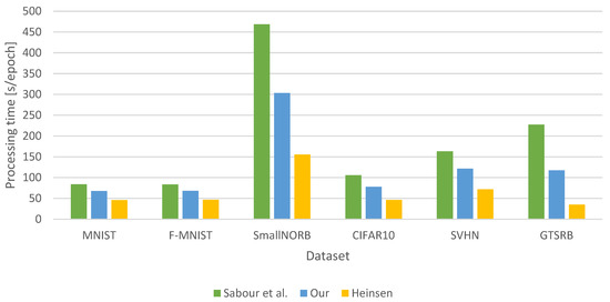
Figure 25.
Comparison of training time on the same hardware (Nvidia Quadro RTX4000 series).
The test errors during the training process are shown in Table 2, where the capsule-based solutions were compared with the recently released neural network-based approaches. It can be clearly seen that our proposed modifications to the routing algorithm have led to efficiency gains. It is important to note that our capsule-based solution does not always approach the effectiveness of the state-of-the-art solutions, however, the capsule network used consists of only three layers with a very minimal number of parameters (). Its architecture is quite simple, but with further improvements, a higher efficiency can be achieved. Prior to this, we felt it necessary to improve the efficiency of the routing algorithm. Experience has shown that designing deep network architecture in the area of capsule networks is too resource-intensive. For this reason, it is necessary to increase the processing speed of the routing algorithm.
Table 2.
Classification test errors on the different datasets, compared with other methods.
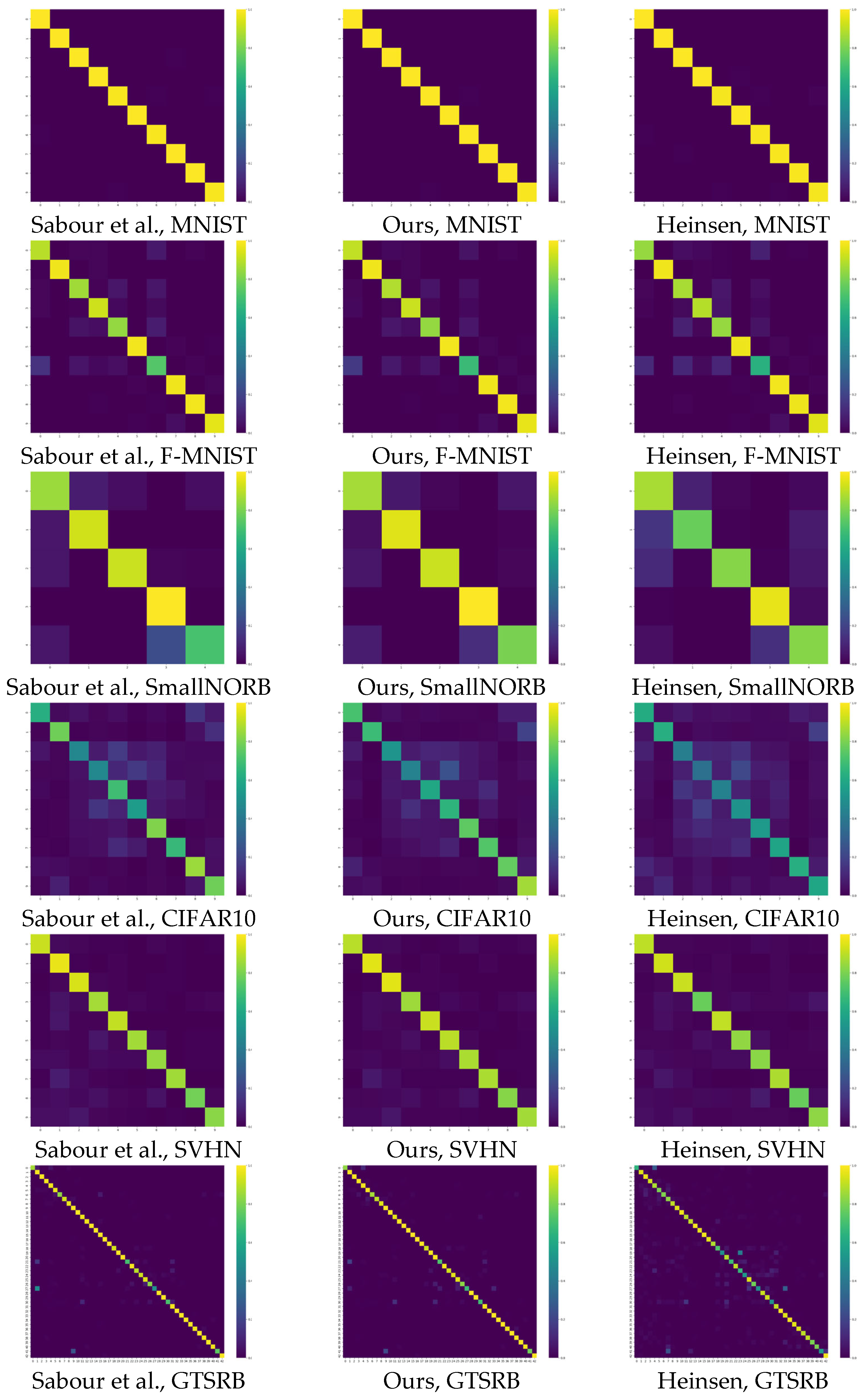
Figure 26 shows the confusion matrices for the capsule network-based approaches in the case of the datasets used. It can be seen that for simpler datasets, such as MNIST, the difference between the three optimization algorithms is minimal. For more complex datasets, the differences are more pronounced. Table 3, Table 4, Table 5, Table 6, Table 7 and Table 8 show the efficiencies achieved by capsule networks for each class, separately. This table also shows that our proposed method is in most cases able to provide a more effective solution than the other solutions tested. However, there are cases where our solution falls short compared with solutions by Sabour et al. and Heinsen.
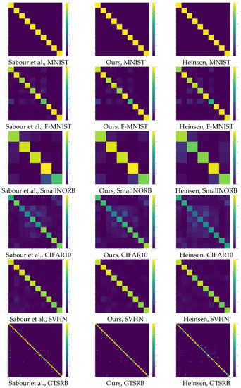
Figure 26.
Confusion matrices for the capsule-based networks.
Table 3.
Classification test accuracy by class for capsule networks on the MNIST dataset.
Table 4.
Classification test accuracy by class for capsule networks on the Fashion-MNIST dataset.
Table 5.
Classification test accuracy by class for capsule networks on the CIFAR10 dataset.
Table 6.
Classification test accuracy by class for capsule networks on the SmallNORB dataset.
Table 7.
Classification test accuracy by class for capsule networks on the GTSRB dataset.
Table 8.
Classification test accuracy by class for capsule networks on the SVHN dataset.
Table 9 summarizes the percentage of classes per dataset that were able to provide the best result for a given solution. From this approach as well, our solution performed the best. Only in the case of the GTSRB dataset was the method proposed by Sabour et al. more efficient. For the other datasets, our proposed method was able to achieve the best accuracy for most classes. Table 10, Table 11 and Table 12 summarize the recall score, dice score and F1-score for the capsule-based implementations under study. It can be observed that, according to all three metrics, our proposed method performs the best. The solution by Sabour et al. performs better only for the Fashion-MNIST dataset, but there was no difference in accuracy of this dataset. The solution by Heinsen underperforms the other two solutions in the cases studied. It can also be seen that, where the method of Sabour et al. and our approach perform worse, the score of Heinsen’s solution also decreases in a similar way.
Table 9.
Best efficiency ratio per class for the presented capsule networks.
Table 10.
Recall scores for the capsule networks.
Table 11.
Dice scores for the capsule networks.
Table 12.
F1-scores for the capsule networks.
7. Conclusions
Our work involved research in the field of capsule networks. We showed the main differences between classical convolutional neural networks and capsule networks, highlighting the new potential of capsule networks. We have shown that the dynamic routing algorithm for capsule networks is too complex and that the training time makes it difficult to build more deep and complex networks. At the same time, capsule networks can achieve very good efficiency, but their practical application is difficult due to the complexity of routing. Therefore, it is important to improve the optimization algorithm and introduce novel solutions.
We proposed a modified routing algorithm for capsule networks and a parameterizable activation function for capsules, based on the dynamic routing algorithm introduced by Sabour et al. In this approach, we aimed to reduce the computational complexity of the current dynamic routing algorithm. Thanks to our proposed routing algorithm and activation function, the training time can be reduced. In our work, we have shown its effectiveness on different datasets, compared with neural network-based solutions and capsule-based solutions. As can be seen, the training time was reduced in all cases, by almost on average. Even in the worst case, a speed increase of almost was achieved. And in some cases, an increase in speed of almost can be seen. Despite the increase in speed, the efficiency of the network has not decreased. For several different metrics, our proposed solution was compared with other capsule-based methods. As we have shown, our proposed approach can increase the efficiency of the routing mechanism. For all six datasets tested in this research, our solution provided the highest results in almost all cases.
In the future, we would like to perform further research on routing algorithms and capsule networks to be able to achieve even greater improvements. We would like to carry out more complex studies on larger datasets, compared with other solutions. We would like to further optimize our solution based on the test results. Our goal is to be able to provide an efficient and fast solution for more complex tasks, such as instance segmentation or reconstruction, in the field of capsule networks. This is necessary to create much deeper and more complex capsule networks, so it is important to address the issue of optimization. This will allow us to apply the theory of capsule networks to real practical applications with great efficiency.
Author Contributions
Conceptualization, J.H., Á.B. and C.R.P.; methodology, J.H., Á.B. and C.R.P.; software, J.H.; validation, J.H.; formal analysis, J.H.; investigation, J.H.; resources, J.H.; data curation, J.H.; writing—original draft preparation, J.H.; writing—review and editing, J.H.; visualization, J.H.; supervision, Á.B. and C.R.P.; project administration, J.H.; funding acquisition, J.H. and Á.B. All authors have read and agreed to the published version of the manuscript.
Funding
This research was funded by the European Union within the framework of the National Laboratory for Artificial Intelligence grant number RRF-2.3.1-21-2022-00004 and the APC was funded by RRF-2.3.1-21-2022-00004.
Data Availability Statement
Data sharing is not applicable.
Acknowledgments
The research was supported by the European Union within the framework of the National Laboratory for Artificial Intelligence (RRF-2.3.1-21-2022-00004).
Conflicts of Interest
The authors declare no conflict of interest.
References
- Chen, X.; Liang, C.; Huang, D.; Real, E.; Wang, K.; Liu, Y.; Pham, H.; Dong, X.; Luong, T.; Hsieh, C.; et al. Symbolic Discovery of Optimization Algorithms. arXiv 2023, arXiv:2302.06675. [Google Scholar]
- Dosovitskiy, A.; Beyer, L.; Kolesnikov, A.; Weissenborn, D.; Zhai, X.; Unterthiner, T.; Dehghani, M.; Minderer, M.; Heigold, G.; Gelly, S.; et al. An Image is Worth 16x16 Words: Transformers for Image Recognition at Scale. In Proceedings of the International Conference on Learning Representations (ICLR), Vienna, Austria, 4 May 2021. [Google Scholar]
- Wang, W.; Dai, J.; Chen, Z.; Huang, Z.; Li, Z.; Zhu, X.; Hu, X.; Lu, T.; Lu, L.; Li, H.; et al. InternImage: Exploring Large-Scale Vision Foundation Models with Deformable Convolutions. arXiv 2023, arXiv:2211.05778. [Google Scholar]
- Ghiasi, G.; Cui, Y.; Srinivas, A.; Qian, R.; Lin, T.; Cubuk, E.D.; Le, Q.V.; Zoph, B. Simple Copy-Paste is a Strong Data Augmentation Method for Instance Segmentation. In Proceedings of the Computer Vision and Pattern Recognition Conference (CVPR), online, 19–25 June 2021. [Google Scholar]
- Su, W.; Zhu, X.; Tao, C.; Lu, L.; Li, B.; Huang, G.; Qiao, Y.; Wang, X.; Zhou, J.; Dai, J. Towards All-in-one Pre-training via Maximizing Multi-modal Mutual Information. arXiv 2022, arXiv:2211.09807. [Google Scholar]
- Yuan, Y.; Chen, X.; Chen, X.; Wang, J. Segmentation Transformer: Object-Contextual Representations for Semantic Segmentation. In Proceedings of the European Conference on Computer Vision (ECCV), Online, 23–28 August 2020. [Google Scholar]
- Fang, Y.; Wang, W.; Xie, B.; Sun, Q.; Wu, L.; Wang, X.; Huang, T.; Wang, X.; Cao, Y. EVA: Exploring the Limits of Masked Visual Representation Learning at Scale. arXiv 2022, arXiv:2211.07636. [Google Scholar]
- Zhang, H.; Li, F.; Zou, X.; Liu, S.; Li, C.; Gao, J.; Yang, J.; Zhang, L. A Simple Framework for Open-Vocabulary Segmentation and Detection. arXiv 2023, arXiv:2303.08131. [Google Scholar]
- Zafar, A.; Aamir, M.; Mohd Nawi, N.; Arshad, A.; Riaz, S.; Alruban, A.; Dutta, A.K.; Almotairi, S. A Comparison of Pooling Methods for Convolutional Neural Networks. Appl. Sci. 2022, 12, 8643. [Google Scholar] [CrossRef]
- Hinton, G.E.; Krizhevsky, A.; Wang, S.D. Transforming Auto-Encoders. International Conference on Artificial Neural Networks; Lecture Notes in Computer Science; Springer: Berlin/Heidelberg, Germany, 2011; Volume 6791, pp. 44–51. [Google Scholar]
- Sabour, S.; Frosst, N.; Hinton, G.E. Dynamic Routing Between Capsules. In Proceedings of the 31st Conference on Neural Information Processing Systems (NIPS), Long Beach, CA, USA, 4–7 December 2017. [Google Scholar]
- Hinton, G.E.; Sabour, S.; Frosst, N. Matrix capsules with EM routing. In Proceedings of the 6th International Conference on Learning Representations, Vancouver, BC, Canada, 30 April–3 May 2018. [Google Scholar]
- LeCun, Y.; Cortes, C.; Burges, C.J.C. The MNIST Database of Handwritten Digits. 2012. Available online: http://yann.lecun.com/exdb/mnist/ (accessed on 9 April 2023).
- Fukushima, K. Visual Feature Extraction by a Multilayered Network of Analog Threshold Elements. In IEEE Transactions on Systems Science and Cybernetics, October 1969; IEEE: Piscataway, NJ, USA, 1969; Volume 5, pp. 322–333. [Google Scholar]
- Xiao, H.; Rasul, K.; Vollgraf, R. Fashion-MNIST: A Novel Image Dataset for Benchmarking Machine Learning Algorithms. arXiv 2017, arXiv:1708.07747. [Google Scholar]
- LeCun, Y.; Huang, F.J.; Bottou, L. Learning methods for generic object recognition with invariance to pose and lighting. In Proceedings of the IEEE Computer Society Conference on Computer Vision and Pattern Recognition (CVPR), Washington, DC, USA, 27 June–2 July 2004; pp. 97–104. [Google Scholar]
- Krizhevsky, A. Learning Multiple Layers of Features from Tiny Images; Technical Report; University of Toronto: Toronto, ON, Canada, 2009. [Google Scholar]
- Netzer, Y.; Wang, T.; Coates, A.; Bissacco, A.; Wu, B.; Ng, A.Y. Reading Digits in Natural Images with Unsupervised Feature Learning. In Proceedings of the 25th Conference on Neural Information Processing Systems, Granada, Spain, 12–17 December 2011. [Google Scholar]
- Stallkamp, J.; Schlipsing, M.; Salmen, J.; Igel, C. The German traffic sign recognition benchmark: A multi-class classification competition. In Proceedings of the International Joint Conference on Neural Networks, San Jose, CA, USA, 31 July–5 August 2011; pp. 1453–1460. [Google Scholar]
- Heinsen, F.A. An Algorithm for Routing Vectors in Sequences. arXiv 2022, arXiv:2211.11754. [Google Scholar]
- Rossum, V.G.; Fred, L.D. Python 3 Reference Manual; CreateSpace: Scotts Valley, CA, USA, 2009. [Google Scholar]
- Paszke, A.; Gross, S.; Massa, F.; Lerer, A.; Bradbury, J.; Chanan, G.; Killeen, T.; Lin, Z.; Gimelshein, N.; Antiga, L.; et al. PyTorch: An Imperative Style, High-Performance Deep Learning Library. Adv. Neural Inf. Process. Syst. 2019, 32, 8024–8035. [Google Scholar]
- Paperspace. Available online: https://www.paperspace.com/ (accessed on 9 April 2023).
- Kingma, D.P.; Ba, J. Adam: A Method for Stochastic Optimization. arXiv 2017, arXiv:1412.6980. [Google Scholar]
- Goyal, P.; Duval, Q.; Seessel, I.; Caron, M.; Misra, I.; Sagun, L.; Joulin, A.; Bojanowski, P. Vision Models Are More Robust and Fair When Pretrained On Uncurated Images without Supervision. arXiv 2022, arXiv:2202.08360. [Google Scholar] [CrossRef]
- Taylor, L.; King, A.; Harper, N. Robust and Accelerated Single-Spike Spiking Neural Network Training with Applicability to Challenging Temporal Tasks. arXiv 2022, arXiv:2205.15286. [Google Scholar] [CrossRef]
- Phaye, S.S.R.; Sikka, A.; Dhall, A.; Bathula, D. Dense and Diverse Capsule Networks: Making the Capsules Learn Better. arXiv 2018, arXiv:1805.04001. [Google Scholar] [CrossRef]
- Remerscheid, N.W.; Ziller, A.; Rueckert, D.; Kaissis, G. SmoothNets: Optimizing CNN Architecture Design for Differentially Private Deep Learning. arXiv 2022, arXiv:2205.04095. [Google Scholar] [CrossRef]
- Dupont, E.; Doucet, A.; Teh, Y.W. Augmented Neural ODEs. In Advances in Neural Information Processing Systems; Curran Associates, Inc.: Red Hook, NY, USA, 2019; Volume 32. [Google Scholar]
- Abad, G.; Ersoy, O.; Picek, S.; Urbieta, A. Sneaky Spikes: Uncovering Stealthy Backdoor Attacks in Spiking Neural Networks with Neuromorphic Data. arXiv 2023, arXiv:2302.06279. [Google Scholar] [CrossRef]


Disclaimer/Publisher’s Note: The statements, opinions and data contained in all publications are solely those of the individual author(s) and contributor(s) and not of MDPI and/or the editor(s). MDPI and/or the editor(s) disclaim responsibility for any injury to people or property resulting from any ideas, methods, instructions or products referred to in the content. |
© 2023 by the authors. Licensee MDPI, Basel, Switzerland. This article is an open access article distributed under the terms and conditions of the Creative Commons Attribution (CC BY) license (https://creativecommons.org/licenses/by/4.0/).