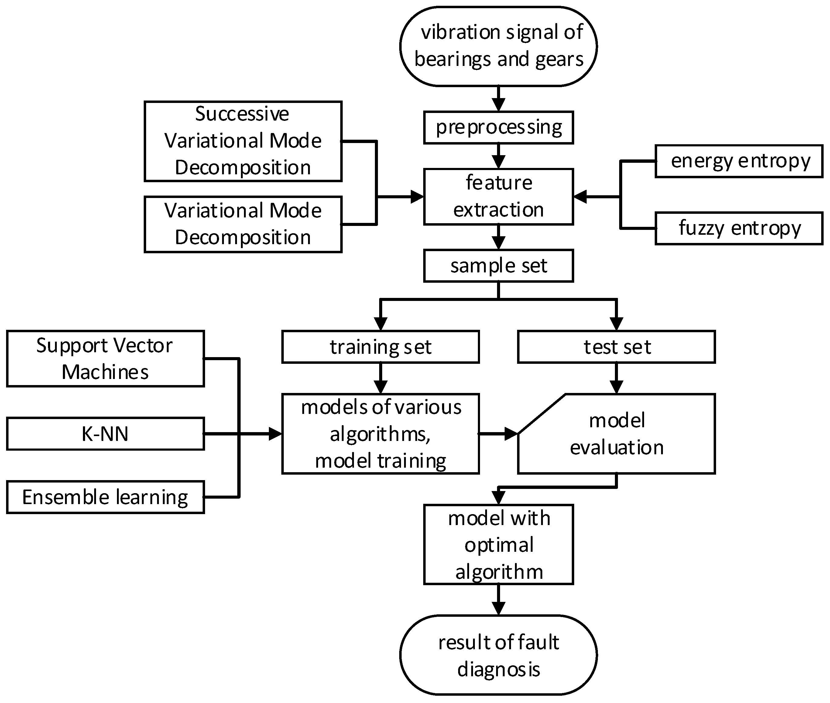
Fault-Diagnosis Method for Rotating Machinery Based on SVMD Entropy and Machine Learning

Abstract

Rolling bearings and gears are important components of rotating machinery. Their operating condition affects the operation of the equipment. Fault in the accessory directly leads to equipment downtime or a series of adverse reactions in the system, which brings enormous pecuniary loss to the institution. Hence, it is of great significance to detect the operating status of rolling bearings and gears for fault diagnosis. At present, the vibration method is considered to be the most common method for fault diagnosis, a method that analyzes the equipment by collecting vibration signals. However, rotating-machinery fault diagnosis is challenging due to the need to select effective fault feature vectors, use appropriate machine-learning classification methods, and achieve accurate fault diagnosis. To solve this problem, this paper illustrates a new fault-diagnosis method combining successive variational-mode decomposition (SVMD) entropy values and machine learning. First, the simulation signal and the real fault signal are used to analyze and compare the variational-mode decomposition (VMD) and SVMD methods. The comparison results prove that SVMD can be a useful method for fault diagnosis. Then, these two methods are utilized to extract the energy entropy and fuzzy entropy of the gearbox dataset of Southeast University (SEU), respectively. The feature vector and multiple machine-learning classification models are constructed for failure-mode identification. The experimental-analysis results successfully verify the effectiveness of the combined SVMD entropy and machine-learning approach for rotating-machinery fault diagnosis.

1. Introduction

As the core components of rotating machinery, rolling bearings have the characteristics of complex structure, high running speed, and large load. However, they have high requirements for precision and are very sensitive to materials such as metal crumbs. Gears are characterized by high working accuracy, a wide application range, and excellent efficiency. However, the manufacturing, installation, and environmental requirements are high. Therefore, rolling bearings and gears have various types of failures and are fragile. Taking wind turbines as an example, as they work in the field and complex environments where temperature and humidity are volatile and loads are unstable, the operational equipment is under heavy stress, which results in a higher probability of damage to rotating parts of wind turbines and high potential maintenance costs [1,2]. Studies have shown that rolling bearings account for 30% of failures in the mechanical drive of wind turbines [3,4]. In addition, an annual check of 40% of train bearings found that one third of them need to be replaced. Meanwhile, gears are easily damaged, accounting for approximately 10% of all rotating-machinery failures [5,6].

In the process of fault diagnosis, the collected vibration signals are used to estimate the occurrence of the fault. However, the collected fault-vibration signals are characterized by nonlinear and non-smooth status. An algorithm is required to decompose the fault-vibration signals into multiple smooth signals and extract the feature signals. Therefore, a series of signal-decomposition algorithms was developed [7] that greatly promoted the development of theoretical research and engineering applications in the field of fault diagnosis.

The requirement of wavelet-transform application is restricted and requires expert a priori knowledge. The mother wavelet and decomposition levels in particular need to be manually determined in advance [8]. Local mean decomposition (LMD) is highly affected by noise and adds redundant frequency components when performing signal decomposition [9]. The mechanical-fault-diagnosis method based on empirical-mode decomposition (EMD) [10,11,12] can adaptively extract the mode components of the local eigen structure of the signal. Ensemble empirical-mode decomposition (EEMD) is a noise-assisted signal-analysis method that is added to EMD to improve the mode-aliasing phenomenon in signal decomposition [13,14]. Complete ensemble empirical-mode decomposition with adaptive noise (CEEMDAN) is an improved EEMD method and has better performance in signal denoising [15,16]. Intrinsic time-scale decomposition (ITD) can suppress endpoint effects more effectively and has good computational efficiency compared with EMD and LMD; however, ITD also has problems with distorting some signals during decomposing. In addition, the quality requirements of the signal are high [17,18]. Variational-mode decomposition (VMD) is a signal-processing method proposed by Dragomiretskiy [19] that has strong robustness to noise and excellent performance [20,21,22]. In recent years, many improved algorithms for VMD have been studied, but the problem of under-decomposition inevitably is caused by the limitations of the algorithm [23,24,25]. Kim presented real case studies of fault diagnosis based on deep convolutional networks and principal component analysis [26,27]. Regarding the topic of fault diagnosis for rotating machinery, many studies have been conducted; however, the following difficulties and challenges are posed:

• Selection of fault-feature vectors. Effective fault-feature vectors are crucial for rotating-machinery fault diagnosis, but it is challenging to choose the right ones due to the many types of faults and their corresponding feature vectors.
• Machine-learning classification methods. Machine-learning algorithms are used for classification, but it is challenging to choose the appropriate algorithm, adjust the hyperparameters, and handle the problem of data imbalance due to the small amount of fault data and the imbalance of sample sizes for different fault types.
• Accurate fault diagnosis. Accurately diagnosing faults is the main goal, but it is challenging due to the need to analyze the fault-feature vectors and machine-learning classification results, select different diagnosis methods for different fault types, and achieve real-time diagnosis during operation.

This paper proposes a new fault-diagnosis method combing successive variational-mode decomposition (SVMD) [28] entropy values and machine learning, which allows for continuous extraction of modes when the number of modes is unknown. This method, similar to the VMD method, treats the modes as the most spectrally compact signals and achieves mode decomposition by adding criteria to deal with the VMD-optimization problem. In this paper, the new method is validated using simulation data. The results show that the new method can basically converge to the same pattern of modes as VMD with a known number of modes, in the case where the number of modes is unknown.

The sections of this paper are organized as follows: Section 2 introduces the basic principles of signal-decomposition methods such as VMD and SVMD, and illustrates the effects of signal decomposition with simulated signals as examples. Section 3 focuses on the fault-specific feature-extraction methods of energy entropy and fuzzy entropy. Section 4 details the experimental dataset, experimental results, and related discussions. The discussion and open issues for future directions are presented in Section 5. Section 6 provides the conclusions of the whole study.

2. Signal-Decomposition Methods

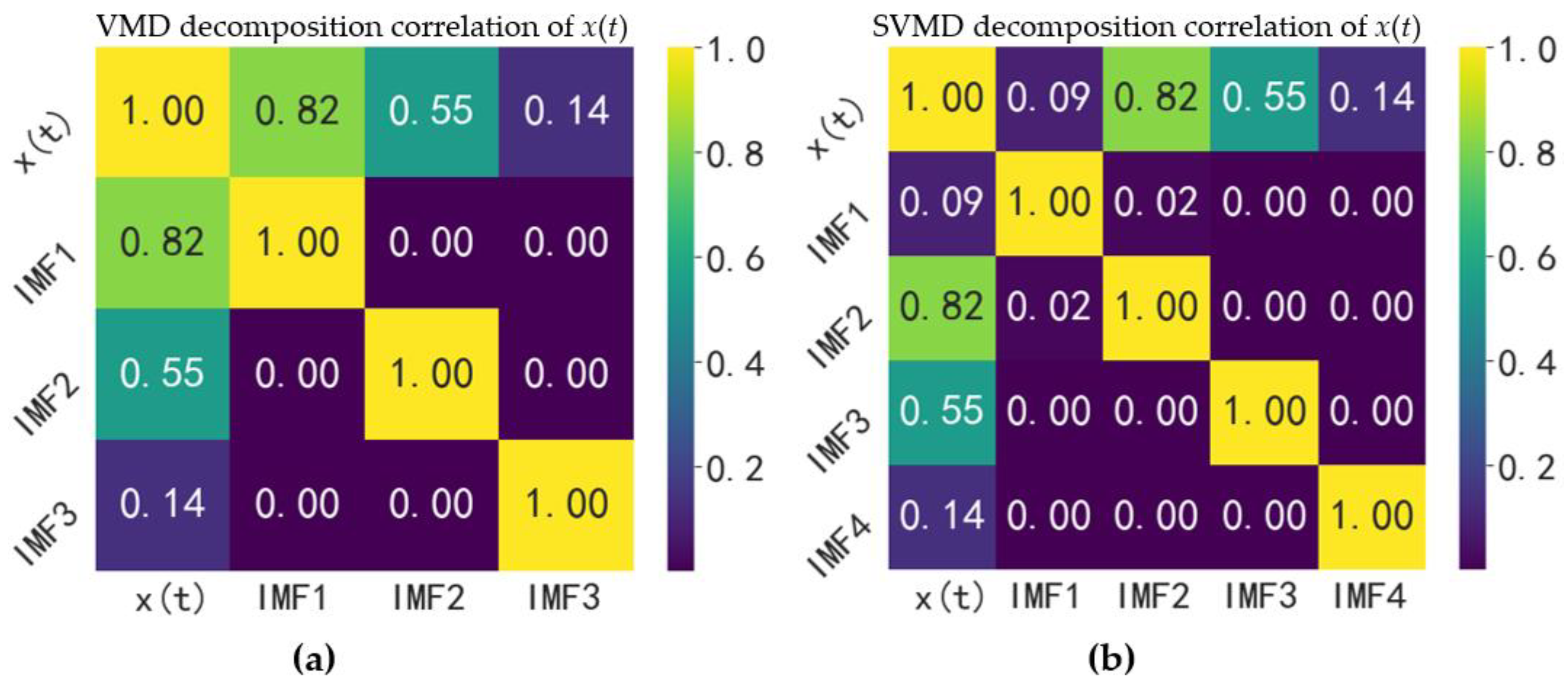
2.1. Variational-Mode Decomposition (VMD)

In the VMD algorithm, the intrinsic-mode function (IMF) is redefined as an AM–FM signal with Equation (1):

$$u_k\left(t\right)=A_k\left(t\right)cos\left({\Phi }_k\right(t\left)\right)$$

(1)

where $A_k\left(t\right)$ is the instantaneous amplitude of $u_k\left(t\right)$; ${\Phi }_k\left(t\right)$ is the instantaneous phase of $u_k\left(t\right)$.

When the VMD algorithm obtains the IMF component, it gets rid of the circular-sieving and stripping-signal-processing method used by the EMD algorithm and transfers the signal-decomposition process to the variational framework, realizing the adaptive decomposition of the signal by searching for the optimal solution of the constrained variational model. The frequency center and bandwidth of each IMF component are constantly updated in the process of iteratively solving the variational model. Finally, the adaptive division of the signal-frequency band can be completed according to the frequency-domain characteristics of the actual signal, and several narrowband IMF components can be obtained. Assuming that the original signal is decomposed into K IMF components, the corresponding expression of the constrained variational model is as follows:

$$\underset{u_k{,\omega }_k}{\min }\left\{\begin{array}{c}{\sum }_k{‖{\partial }_t\left[\left(\delta \left(t\right)+\frac{i}{\pi t}\right)u_k\left(t\right)\right]e^{-i{\omega }_{k}t}‖}_2^2\\ {\sum }_k{u}_k=f\end{array}\right\}$$

(2)

where $u_k$ represents K IMF components obtained by the decomposition, ${\omega }_k$ denotes the central frequency of each component, and $\delta \left(t\right)$ is the Dirac function.

To find the optimal solution of the above constrained variational problem, an incremental Lagrange function of the following form is introduced:

$$\begin{gathered} L(u_k,{\omega }_k,\lambda )=\alpha {\sum }_k{‖{\partial }_t\left[\left(\delta (t)+\frac{i}{\pi t}\right)u_k(t)\right]e^{-i{\omega }_{k}t}‖}_2^2 \\ +{‖f(t)-{\sum }_k{u}_k(t)‖}_2^2+〈\lambda (t),f(t)-{\sum }_k{u}_k(t)〉 \end{gathered}$$

(3)

where $\alpha$ is the penalty factor, and $\lambda$ is the Lagrange multiplier.

The alternating direction-multiplier algorithm is used to find the saddle point of the above incremental Lagrange function, which is the optimal solution of the constrained variational model of Equation (3), so as to decompose the original signal into K narrowband IMF components. The specific implementation process is as follows.

(1)

Initialize $u_k^1$, ${\omega }_k^1$, ${\lambda }^1$, and n to 0.

(2)

n = n + 1; execute the entire loop.

(3)

Execute the first loop of the inner level based on $u_k^{n+1}={\arg }_{u_k}\min L(u_{i<k}^{n+1}{, \lambda }^n$, $u_{i\ge k}^n$, ${\omega }_i^n$) and update $u_k$.

(4)

k = k + 1 and repeat step (3) until k = K; then end the first loop of the inner layer.

(5)

Execute the second loop of the inner level based on ${\omega }_k^{n+1}={\arg }_{{\omega }_k}\min L\left(u_i^{n+1}, {\omega }_{i<k}^{n+1}, {\omega }_{i\ge k}^{n+1}, {\lambda }^n\right)$ and update ${\omega }_k$.

(6)

k = k + 1 and repeat step (5) until k = K, then end the second loop in the inner layer.

(7)

Based on ${\lambda }^{n+1}={\lambda }^n+\tau (f-{\sum }_k{u}_k^{n+1})$, update $\lambda$.

(8)

Repeat steps (2)$~$(7) until the iteration-stop condition $\sum _k({‖u_k^{n+1}-u_k^n‖}_2^2/{‖u_k^n‖}_2^2)<\epsilon$ is satisfied, end the whole loop, and output the result to get K narrowband IMF components.

2.2. Successive Variational-Mode Decomposition (SVMD)

SVMD is an efficient and fast signal-variational adaptive-decomposition method that extends variational-mode extraction (VME) [29]. VME is used to extract specific signal modes by approximating the center frequency of the intrinsic mode function. This new decomposition method extracts all modes in a continuous manner. Compared to VMD, this continuous method does not require mode-number information and is highly robust. The specific implementation of VME is as follows.

(1)

Initialize ${\widehat{u}}_d^1$, ${\widehat{\lambda }}^1$, ${\widehat{w}}_d^1$ and $n$ to $0$.

(2)

$n=n+1$; execute the entire loop.

(3)

Update all ${\widehat{u}}_d$, where $w\ge 0$ based on ${\widehat{u}}_d^{n+1}\left(w\right)=\frac{\widehat{f}\left(w\right)-{\alpha }^2{(w-w_d^{n+1})}^4{\widehat{u}}_d^n(w)+\frac{\widehat{\lambda }\left(w\right)}{2}}{\left[1+{\alpha }^2{(w-w_d^{n+1})}^4\right]\left[1+2\alpha {(w-w_d^n)}^2\right]}$.

(4)

Update $w_d$ based on $w_d^{n+1}=\frac{{\int }_0^{\infty }w{\left|{\widehat{u}}_d^{n+1}\left(w\right)\right|}^{2}dw}{{\int }_0^{\infty }{\left|{\widehat{u}}_d^{n+1}\left(w\right)\right|}^{2}dw}$.

(5)

Update $\widehat{\lambda }$, where all $w\ge 0$ base on ${\widehat{\lambda }}^{n+1}={\widehat{\lambda }}^n+\tau \left[\frac{\widehat{f}\left(w\right)-{\widehat{u}}_d^{n+1}\left(w\right)}{1+{\alpha }_m^2{(w-w_d^{n+1})}^4}\right]$.

(6)

Repeat steps (2)$~$(5) until the iteration-stop condition $\frac{{‖{\widehat{u}}_d^{n+1}-{\widehat{u}}_d^n‖}_2^2}{{‖{\widehat{u}}_d^n‖}_2^2}<ϵ$ is satisfied; then end the whole loop and output the result.

The specific implementation process of SVMD is as follows:

(1)

Set parameters ${\alpha }_{min}$, ${\alpha }_{max}$, ${ϵ}_1$, ${ϵ}_2$, and ${\sigma }^2$.

(2)

$L\leftarrow 0$, $L=L+1$; execute the entire loop.

(3)

Set ${\widehat{u}}_L^1$, ${\widehat{\lambda }}^1$, $n=0$, $m=0$, and ${\alpha }_1\leftarrow {\alpha }_{min}$, and $w_L^1$ is initialized to 0 or a random value between 0 and $\pi$.

(4)

$m=m+1$; execute the first loop of the inner level.

(5)

$n=n+1$; execute the second inner loop.

(6)

Update all ${\widehat{u}}_L$, where $w\ge 0$ based on ${\widehat{u}}_L^{n+1}(w)=\frac{\widehat{f}(w)+{(w-w_L^n)}^4{\widehat{u}}_L^n(w)+\frac{\widehat{\lambda }(w)}{2}}{\left[1+{\alpha }_m^2{(w-w_L^n)}^4\right]\left[1+2{\alpha }_m{(w-w_L^n)}^2+\sum _{i=1}^{L-1}\frac{1}{{\alpha }_m^2{(w-w_i)}^4}\right]}$.

(7)

Update $w_L$ based on $w_L^{n+1}=\frac{{\int }_0^{\infty }w{\left|{\widehat{u}}_L^{n+1}\left(w\right)\right|}^{2}dw}{{\int }_0^{\infty }{\left|{\widehat{u}}_L^{n+1}\left(w\right)\right|}^{2}dw}$.

(8)

Update all $\widehat{\lambda }$, where $w\ge 0$ based on ${\widehat{\lambda }}^{n+1}={\widehat{\lambda }}^n+\tau \left[\widehat{f}(w)-\left({\widehat{u}}_L^{n+1}(w)+\left[\frac{{\alpha }_m^2{(w-w_L^{n+1})}^4(\widehat{f}(w)-{\widehat{u}}_L^{n+1}(w)-\sum _{i=1}^{L-1}{\widehat{u}}_i^{n+1}(w)+\frac{\widehat{\lambda }(w)}{2})-\sum _{i=1}^{L-1}{\widehat{u}}_i(w)}{1+{\alpha }_m^2{(w-w_L^{n+1})}^4}\right]+\sum _{i=1}^{L-1}{\widehat{u}}_i^{n+1}\left(w\right)\right)\right]$.

(9)

Repeat steps (5)$~$(8) until the iteration-stop condition $\frac{{‖{\widehat{u}}_L^{n+1}-{\widehat{u}}_L^n‖}_2^2}{{‖{\widehat{u}}_L^n‖}_2^2}<{ϵ}_1$ is satisfied and end the second loop in the inner layer.

(10)

Set ${\widehat{u}}_L^1$, ${\widehat{\lambda }}^1$, $n=0$, $w_L^1=w_L^{n+1}$, and ${\alpha }_{m+1}=2{\alpha }_m$; repeat step (4)$~$(9) until ${\alpha }_{m+1}\le {\alpha }_{max}$ is satisfied; and end the first loop of the inner layer.

(11)

Repeat steps (2)$~$(10) until $\left|{\sigma }^2-\frac{1}{{\rm T}}{‖\left(f\right(t)-{\sum }_{i=1:L}{u}_i\left(t\right))‖}_2^2\right|/{\sigma }^2<{ϵ}_2$ is satisfied, end the whole loop, and output the result.

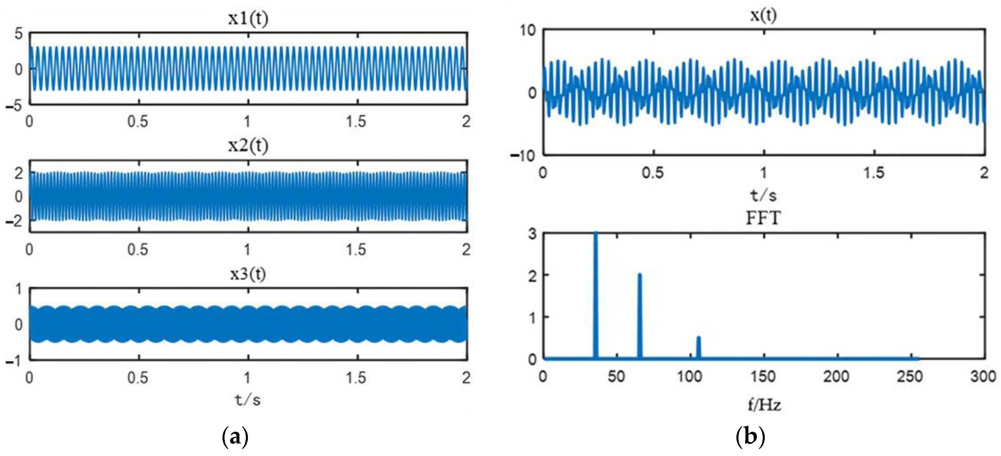
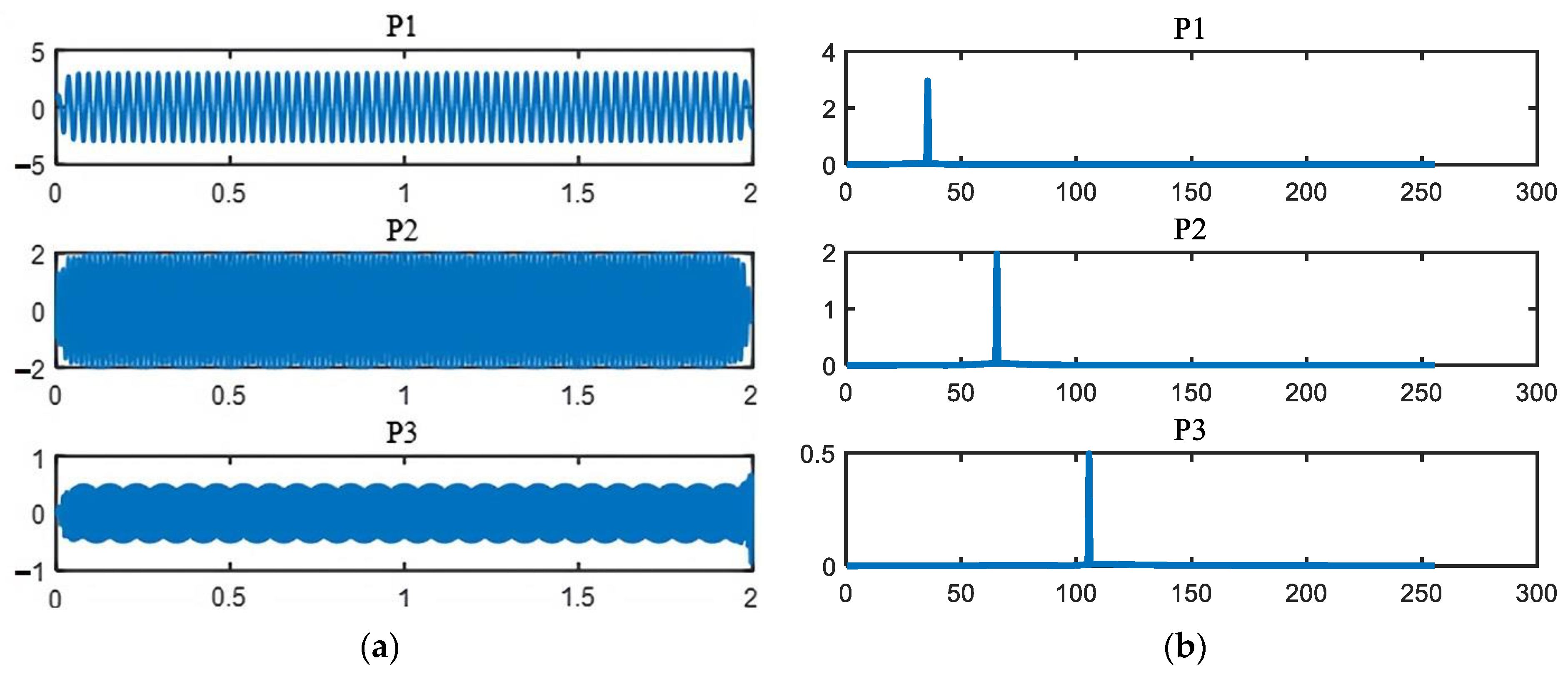
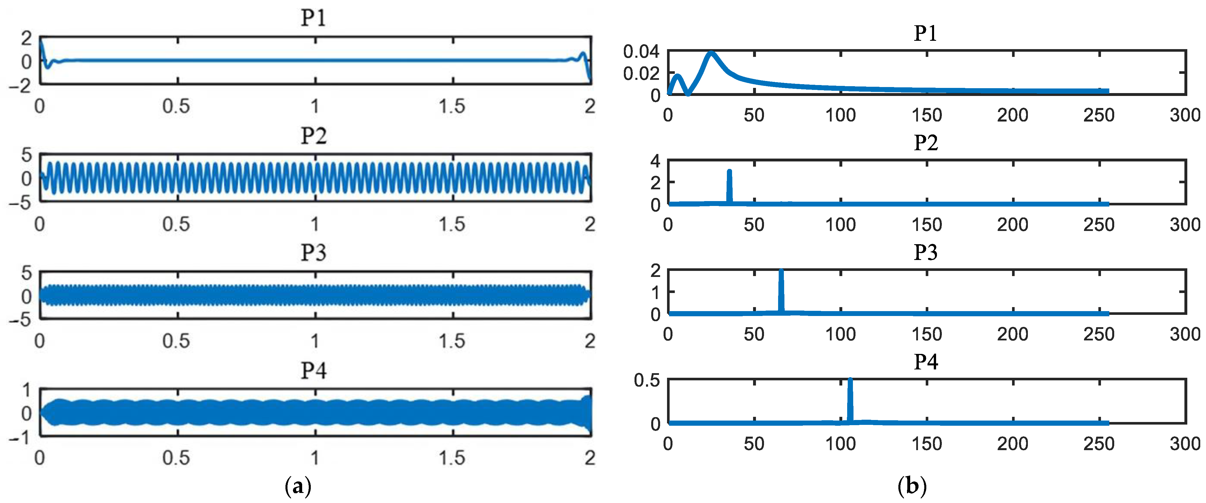
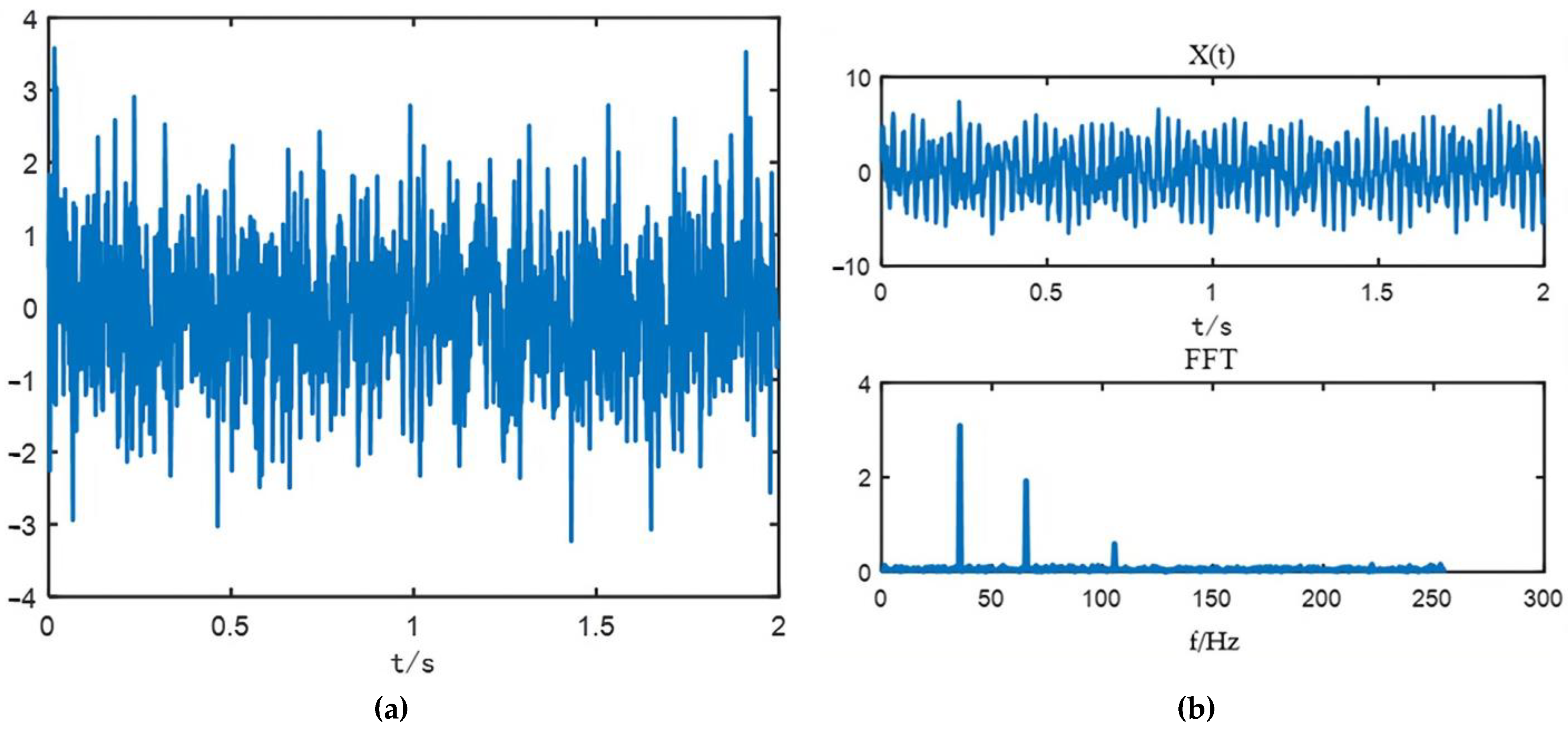
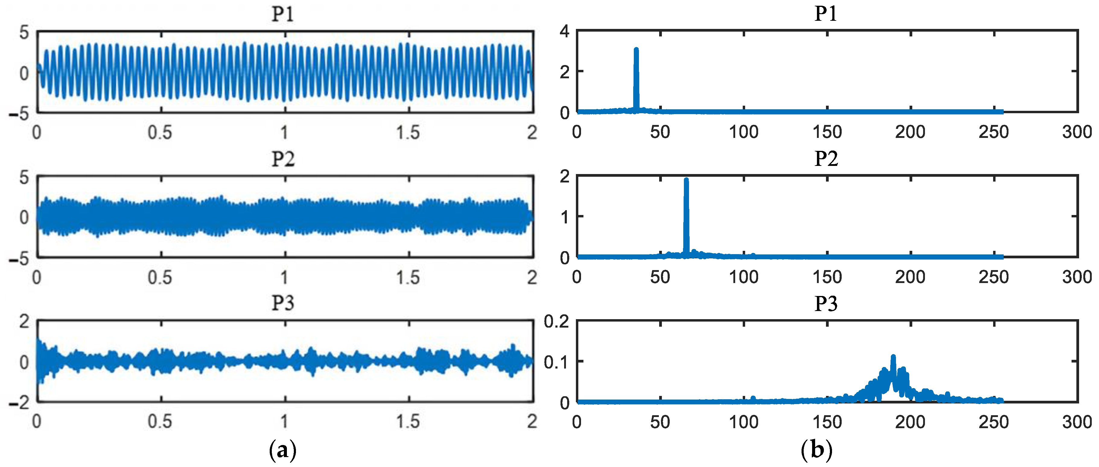
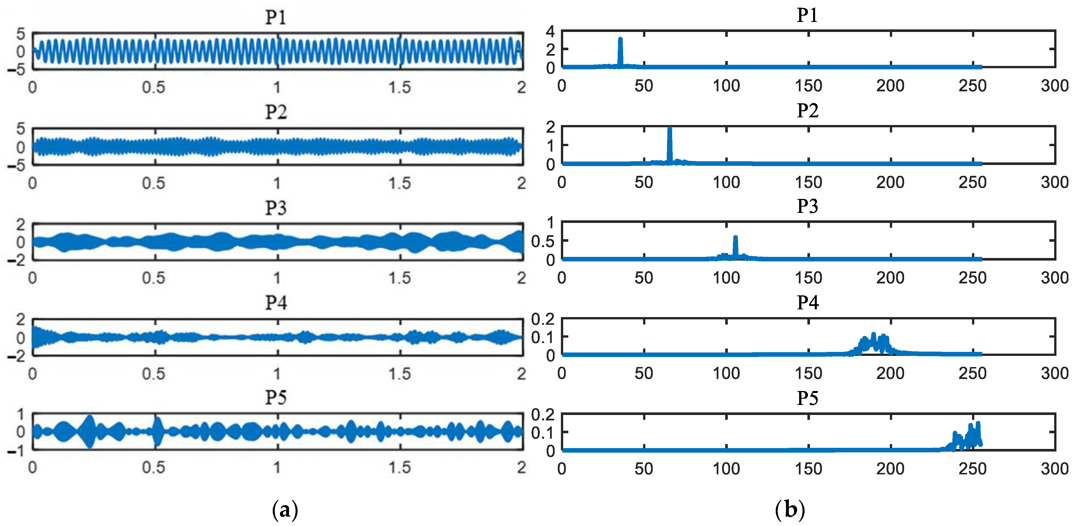
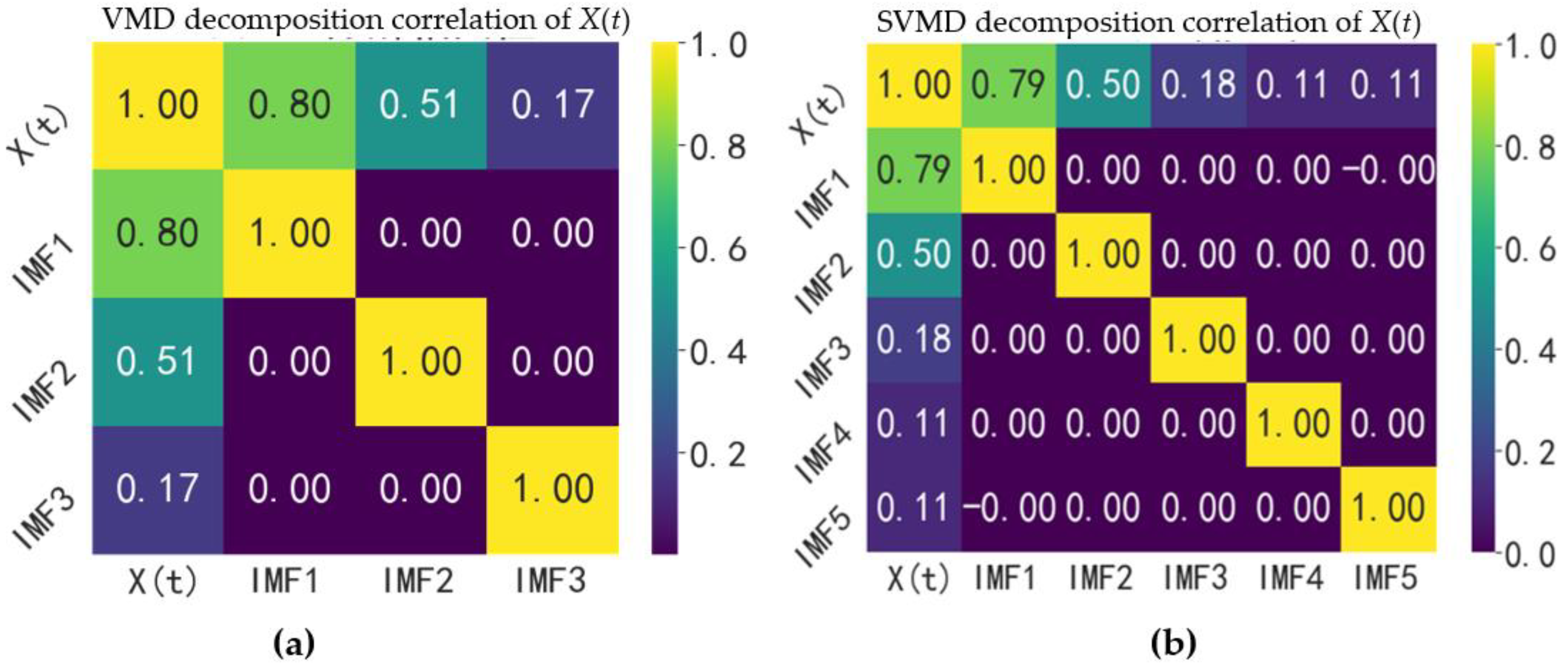
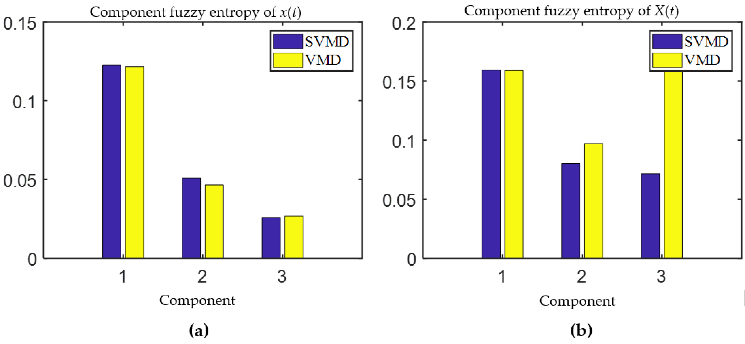
2.3. Simulated Signal Analysis

Create the simulation signal $x\left(t\right)$ as shown in Equations (4) and (5):

$$\left\{\begin{array}{c}x1\left(t\right)=3\ast \sin \left(2\pi 35t\right)\\ x2\left(t\right)=2\ast \sin \left(2\pi 65t\right)\\ x3\left(t\right)=1/2\ast \cos \left(2\pi 105t\right)\end{array}\right\}$$

(4)

$$x\left(t\right)=x1\left(t\right)+x2\left(t\right)+x3\left(t\right)$$

(5)

The time-domain and frequency-domain plots of the simulated signal are shown in Figure 1.

The decomposition of the simulated signal by VMD and SVMD is shown in Figure 2 and Figure 3, respectively. The information on the decomposition of the simulated signal by other signal-decomposition methods is shown in

Table 1. Decomposition of the simulated signal by several signal-decomposition algorithms.

Signal-Decomposition Method	Running Time (s)	Decomposition Fraction (pcs)	Problem
EMD	1.270	7	Mode mixing
LMD	1.857	4	Mode mixing
ITD	1.666	5	Mode mixing
VMD	1.100	3	None
SVMD	1.277	4	One more invalid component

. It can be seen from the figures and tables that VMD had better performance for the simulated signal, SVMD was the second best, and the other methods all showed mode mixing. However, when the value of $K$ was set to 4, mode aliasing occurred.

In the simulated signal $x\left(t\right)$, based on the random function, randn($·$) is superimposed on a random signal composition $X\left(t\right)$. The random signal and $X\left(t\right)$ are shown in Figure 4.

Figure 5 and Figure 6 show the $X\left(t\right)$ signal-decomposition-component of the time-domain–frequency-domain plots for VMD and SVMD, respectively. The statistical results are shown in

Table 2. Decomposition of simulated signals with superimposed random signals by several signal-decomposition algorithms.

Signal-Decomposition Method	Running Time (s)	Decomposition Fraction (pcs)	Problem
EMD	1.692	9	Mode mixing
LMD	2.077	5	All three eigenfrequencies are in the same component
ITD	1.940	7	Mode mixing
VMD	1.558	3	The third characteristic frequency is not effectively separated
SVMD	1.674	5	Invalid fraction exists

. From the experimental results, it can be seen that VMD was the most efficient way to achieve results, but one of the characteristic frequencies could not be separated effectively. The third characteristic frequencies could be separated when the $k$ value was set to 4. SVMD took slightly less time and could separate each feature frequency at one time, which had better robustness. The other methods took more time, had serious mode overlap, and could not separate the feature frequencies effectively.

3. Fault Feature-Extraction Method

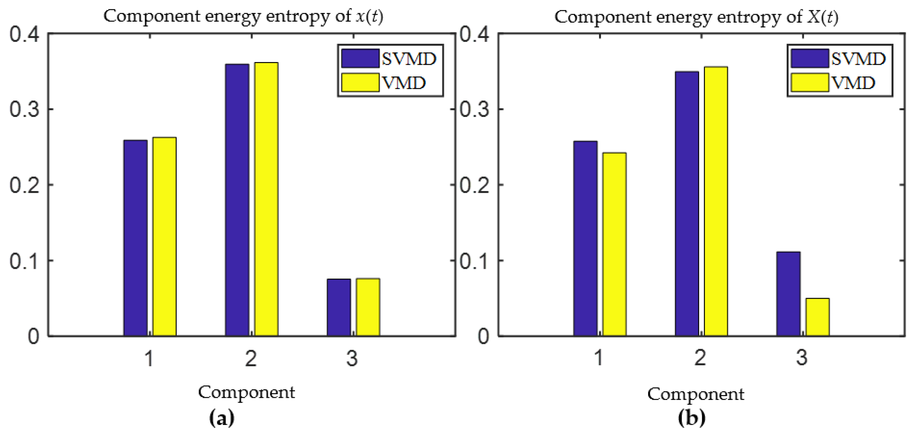
3.1. Energy Entropy

The operation of rolling bearings with different faults produces different resonant-frequency components in the vibration signal. The energy of the fault signal changes in different frequency bands [30]. The IMF components are obtained by decomposing the signal through the adaptive-decomposition method. The energy distribution of each IMF component is different. Therefore, the fault characteristics of the equipment can be characterized by finding the energy entropy of each IMF component.

For the n IMF components decomposed from the vibration signal, $c_1\left(t\right),c_2\left(t\right),\cdots ,c_n\left(t\right)$, and the energy of each component is calculated using Equation (6).

$$E_i={\int }_{-\infty }^{+\infty }{\left|c_i\left(t\right)\right|}^2\mathrm{d}t$$

(6)

Define the energy entropy expressed as:

$$H_{EN}=-\sum _{i=1}^n{p}_i{\log }_2{p}_i$$

(7)

where $p_i=E_i/E$, $E=\sum _{i=1}^n{E}_i$, $x\left(t\right)$ is the simulated signal of Equation (5), and $X\left(t\right)$ is a superimposed random signal by the function randn($·$).

Decomposition of VMD and SVMD is performed to obtain the component-energy entropy, as shown in Figure 7. Figure 7a illustrates that the component-energy entropy of VMD decomposition is basically consistent with that of SVMD decomposition. In addition, it can be seen that the correlations of the IMF1, IMF2, and IMF3 components of VMD decomposition and the correlations of the IMF2, IMF3, and IMF4 components of SVMD decomposition also remained the same. Similarly, the energy entropies of the first two components of $X\left(t\right)$ decomposed by VMD and SVMD from Figure 7b were basically the same, but the IMF3 component of the VMD decomposition was more complex and the eigenfrequencies were masked, at which point its energy-entropy value was half that of the IMF3 component of the SVMD decomposition.

Figure 8 and Figure 9 show the correlation analysis of the simulation signal and components. From Figure 8, it can be seen that the correlation between the components of the VMD decomposition and the simulated signal x(t) was the same size as the correlation between the components of the SVMD decomposition (except IMF1) and the simulated signal x(t), which also indirectly indicates that there was not much difference between the two methods. Similarly, it can be seen from Figure 9 that the correlation between the VMD decomposition components and the simulation signal X(t) remained basically the same as the correlation between the SVMD decomposition components (the first three components), but the IMF3 characteristic frequency of VMD was hidden by other information and it is not easy to determine the effective components if only correlation analysis is performed.

3.2. Fuzzy Entropy

The value of the fuzzy entropy [31] is used to represent the signal complexity, and it uses the mean algorithm and the affiliation-function method to make the similarity measure between vectors fuzzy. The fuzzy entropy is similar to the theoretical properties of sample entropy and approximate entropy, and its fuzzy-entropy value is more stable than when the parameters are changed.

With a set of sampling points of $N$ of sequences $\left\{u\left(i\right):1\le i\le N\right\}$, the fuzzy entropy is solved as follows.

(1)

The sequence is formed as $m$ dimensional vector, as shown in Equation (8):

$$X\left(i\right)=\left\{u\left(i\right), u\left(i+1\right), \cdots , u(i+m-1)\right\}-u_0\left(i\right)$$

(8)

where $i=(1$, $2$, $\cdots$, $N), \mathrm{and} u_0(i)$ is the mean of vector $\left\{u\left(i\right),u\left(i+1\right),\cdots ,u(i+m-1)\right\}$.

(2)

Calculate the maximum amount $d_{ij}$ of the distance difference between the vectors $X_i$ and $X_j$, as shown in Equation (9).

$$d_{ij}=max\left\{\left|X_i-X_j\right|\right\}$$

(9)

(3)

Calculate the similarity $D_{ij}$, which is defined by the exponential function $u$, as shown in Equation (10):

$$D_{ij}=u(d_{ij}, n, r)=exp\left[-{\left(d_{ij}/r\right)}^n\right]$$

(10)

where $u$ is the fuzzy-affiliation function of $X_i$ and $X_j$, and $n$ and $r$ are the gradient and the width of its boundary, respectively.

(4)

Define ${\phi }^m(n,r)$; the result is shown in Equation (11):

$${\phi }^m(n,r)=\frac{1}{N-m}\sum _{i=1}^{N-m}(\frac{1}{N-m+1}\sum _{j=1,j\ne i}^{N-m+1}{D_{ij}}^m)$$

(11)

where the affiliation function ${D_{ij}}^m=e^{-{\left({d_{ij}}^m/r\right)}^n}$, and $r$ is the similarity-tolerance limit.

(5)

Solve the fuzzy-entropy value of $N$ for the infinite value, as shown in Equation (12).

$$FE(m,n,r)=\underset{N\to \infty }{\lim }\left[\ln {\phi }^m(n,r)-\ln {\phi }^{m+1}(n,r)\right]$$

(12)

Generally, $N$ is the finite value, and the above equation is converted as shown in Equation (13).

$$FE(m,n,r)=\ln {\phi }^m(n,r)-\ln {\phi }^{m+1}(n,r)$$

(13)

In the process of fuzzy-entropy calculation, the embedding dimension $m$, threshold $r$, and $n$ are the main factors affecting the accuracy of the calculation, and in this paper $m$ was 3, $r$ was 0.15SD (SD is the standard deviation of the input vibration signal), and $n$ was 2.

Similarly, the fuzzy entropy of the components was obtained by VMD and SVMD decomposition of the simulated signals $x\left(t\right)$ and $X\left(t\right)$, as shown in Figure 10. The fuzzy-entropy values of the components of the VMD decomposition of the simulated signal and the SVMD decomposition remained the same. The fuzzy-entropy value of IMF3 component decomposed by VMD was twice as large as that of IMF3 component decomposed by SVMD, and it can be obviously concluded that the IMF3 component decomposed by VMD was more complicated.

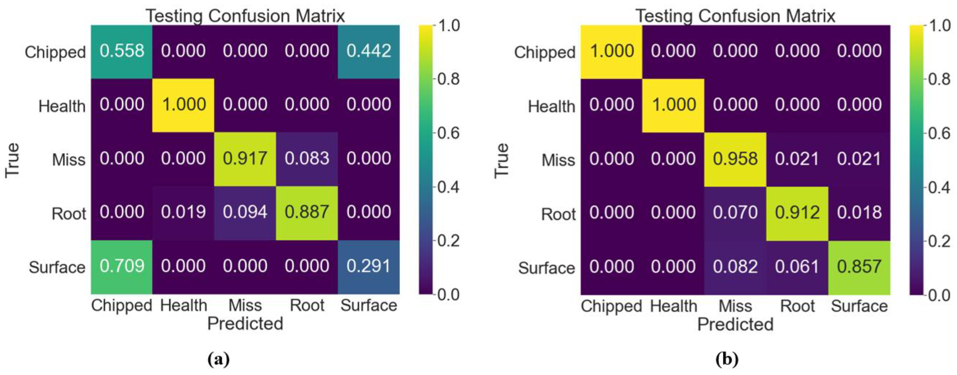
4. Experimental Analysis

In this paper, the above method was investigated through the gearbox-fault-diagnosis dataset of Southeast University (SEU), and the experimental flow is shown in Figure 11.

4.1. SEU Dataset Introduction

The gearbox dataset was from Southeast University (SEU), China. These data were collected from the Drivetrain Dynamic Simulator. This dataset contains two subdatasets, including bearing data and gear data, which were both acquired from the Drivetrain Dynamics Simulator (DDS). There are two kinds of working conditions with the rotating speed-load configurations set to 20-0 and 30-2, which were used to build the separate model. Within each file, there are eight rows of signals, which represent (1) motor vibration; (2, 3, 4) vibration of the planetary gearbox in three directions: x, y, and z; (5) motor torque; and (6, 7, 8) vibration of the parallel gearbox in three directions: x, y, and z. The signals of rows 2, 3, and 4 were all effective. The rolling bearing dataset-failure types were rolling-body failure, inner-ring–outer-ring mixed failure, normal condition, inner-ring failure, and outer-ring failure, as shown in

Table 3. Data set of rolling bearings of SEU.

Operation Conditions	Dataset	Data Length	Fault Type
I	Ball_20_0	1,048,560	Rolling-body failure
	Comb_20_0	1,048,560	Inner-ring and outer-ring mixed failure
	Health_20_0	1,048,560	Normal condition
	Inner_20_0	1,048,560	Inner-ring failure
	Outer_20_0	1,048,560	Outer-ring failure
II	Ball_30_2	1,048,560	Rolling-body failure
	Comb_30_2	1,048,560	Inner-ring and outer-ring mixed failure
	Health_30_2	1,048,560	Normal condition
	Inner_30_2	1,048,560	Inner-ring failure
	Outer_30_2	1,048,560	Outer-ring failure

.

In the planetary-gear dataset, there were five types of broken-tooth faults: normal conditions, missing-tooth faults, root faults, and tooth-surface faults, as shown in

Table 4. Planetary-gear dataset of SEU.

Operation Conditions	Dataset	Data Length	Fault Type
I	Chipped_20_0	1,048,560	Broken-tooth failure
	Health_20_0	1,048,560	Normal condition
	Miss_20_0	1,048,560	Missing-tooth failure
	Root_20_0	1,048,560	Tooth-root failure
	Surface_20_0	1,048,560	Tooth-surface failure
II	Chipped_30_2	1,048,560	Broken-tooth failure
	Health_30_2	1,048,560	Normal condition
	Miss_30_2	1,048,560	Missing-tooth failure
	Root_30_2	1,048,560	Tooth-root failure
	Surface_30_2	1,048,560	Tooth-surface failure

.

4.2. Analytical Comparison

The energy entropy and fuzzy entropy of each component were obtained by decomposing the bearing- and gear-vibration signals through VMD and SVMD. Each of them was constructed into an energy-entropy sample set and a fuzzy-entropy sample set. A machine-learning [32,33] classification model was established to perform intelligent diagnosis of faults.

Firstly, the gear data of two working conditions of the SEU dataset were be studied, and the data length of each class of gear was 1,048,560. This paper took the length of 4096 as a data sample, which could be divided into 255 in total, and then used the VMD and SVMD methods for mode decomposition of each data sample.

When computing energy entropy and fuzzy entropy as feature vectors, it is generally sufficient to take the first six components. The disadvantage of choosing more or fewer components is that choosing more components can increase the computation burden and may lead to overfitting problems, where the model performs well on training data but poorly on unknown data. Additionally, too many components can increase the complexity of the model, making it harder to interpret and understand. Choosing fewer components may result in the loss of important information and a decrease in model accuracy. Therefore, selecting an appropriate number of components, specifically the first six orders, can ensure model accuracy while avoiding issues of excessive complexity and computational burden. Therefore, in this paper, we sought the energy-entropy value and fuzzy-entropy value of the first six components. There were five types of gears. The final composition of the energy-entropy and fuzzy-entropy sample-set size was 1275 × 6 (the former represents rows and the latter represents columns, except for labeled columns). In this paper, there were no training datasets, and all data were used for testing.

Then, a machine-learning classification model was built for pattern recognition. Figure 12 and Figure 13 show the diagnostic effect of the support-vector machine (SVM) [34] in the form of a confusion matrix for the sample set of energy entropy and fuzzy entropy of the SEU gearwork data. The parameters of the two classification models were derived in the form of a grid search. In the SVM model, the penalty factor was [0.01, 0.1, 1, 10, 100] and the kernel-function parameter was [0.01, 0.1, 1, 10, 100]. Here, the optimal parameters were 100 and 100. It was also found that the SVM classification effect of SVMD energy entropy was better than that of VMD energy entropy, whereas the SVM classification effect of the VMD fuzzy-entropy and the SVMD fuzzy-entropy classification effect was about the same.

For the SVM and k-nearest neighbors (k-NN) [35] classification methods, in general, the classification accuracy of SVM is higher than that of k-NN. However, for smaller datasets, k-NN can obtain the same results as SVM or even better. In this paper’s dataset, the number of samples was sourced from the same time series and the sample differences were small, so the results obtained by k-NN were slightly better than those obtained by SVM. In addition, k-NN and SVM can be applied without using a large amount of data for model training and can obtain better models quickly.

Integrated learning is a good strategy to achieve learning by combining multiple learners, both on datasets with large and small amounts of data. The current integrated learning methods can be broadly classified into two categories: One is sequential integration methods, such as boosting in AdaBoost and gradient-boost decision tree (GBDT) [36]. The other is parallel integration methods, such as bagging and random forest (RF) [37].

The classification results of the energy-entropy and fuzzy-entropy sample sets obtained from the VMD and SVMD decompositions of the bearing data in the gearbox of SEU in the SVM, k-NN, RF, and GBDT models are shown in

Table 5. Accuracy of gearbox bearing data at SEU.

Data	Gearbox Bearing Data of SEU
Operation Condition	Operation Condition I				Operation Condition II
Model	SVM	k-NN	RF	GBDT	SVM	k-NN	RF	GBDT
VMD energy entropy	97.57%	97.34%	98.04%	98.04%	97.25%	96.86%	96.08%	97.25%
SVMD energy entropy	97.25%	96.86%	96.47%	97.25%	94.12%	93.33%	91.76%	94.51%
VMD fuzzy entropy	99.13%	98.98%	99.22%	99.22%	99.61%	92.16%	99.61%	99.22%
SVMD fuzzy entropy	93.96%	99.22%	99.22%	99.22%	94.90%	97.25%	95.69%	95.29%

. The table shows that the accuracy of the SVMD fuzzy entropy k-NN, RF, and GBDT models in the gearbox working condition I data of SEU was the same as that of the VMD fuzzy-entropy RF and GBDT models, reaching 99.22%; the accuracy of the VMD fuzzy-entropy SVM and RF models in the working condition II data was the highest, reaching 99.61%.

The SVMD feature-extraction (energy entropy, fuzzy entropy) machine learning in this paper was compared with the machine-learning classification results in the literature [38], as shown in

Table 6. Comparison of SVMD feature extraction and classification results and those from other literature.

	Algorithm	Component: Bearing		Component: Gear
		20-0	30-2	20-0	30-2
Literature [36]	K-NN	80.80%	86.40%	93.20%	89.20%
	SVM	83.30%	88.60%	94.40%	90.10%
Our paper	SVMD fuzzy entropy + k-NN	99.22%	97.25%	94.42%	90.98%
	SVMD energy entropy + SVM	97.25%	94.12%	91.27%	90.20%
	SVMD fuzzy entropy + RF	99.22%	95.69%	96.02%	93.33%
	SVMD fuzzy entropy + GBDT	99.22%	95.29%	95.22%	89.41%

. From the table, it can be seen that in the fault diagnosis of the bearing, the machine-learning classification effect of the SVMD method was better than the identification result of this data in the literature, and in the gearbox, the two were difficult to distinguish.

In the paper, the grid-search method was also chosen to select the two model parameters of RF and GBDT. When performing the grid search, the n_estimators parameter and the max_depth parameter in RF were both set to integers between 5 and 13, the min_samples_split parameter was set to 2, and other parameters were set by default. In GBDT, the n_estimators parameter was set to an integer between 50 and 150 with an interval of 10, and other parameters were set by default.

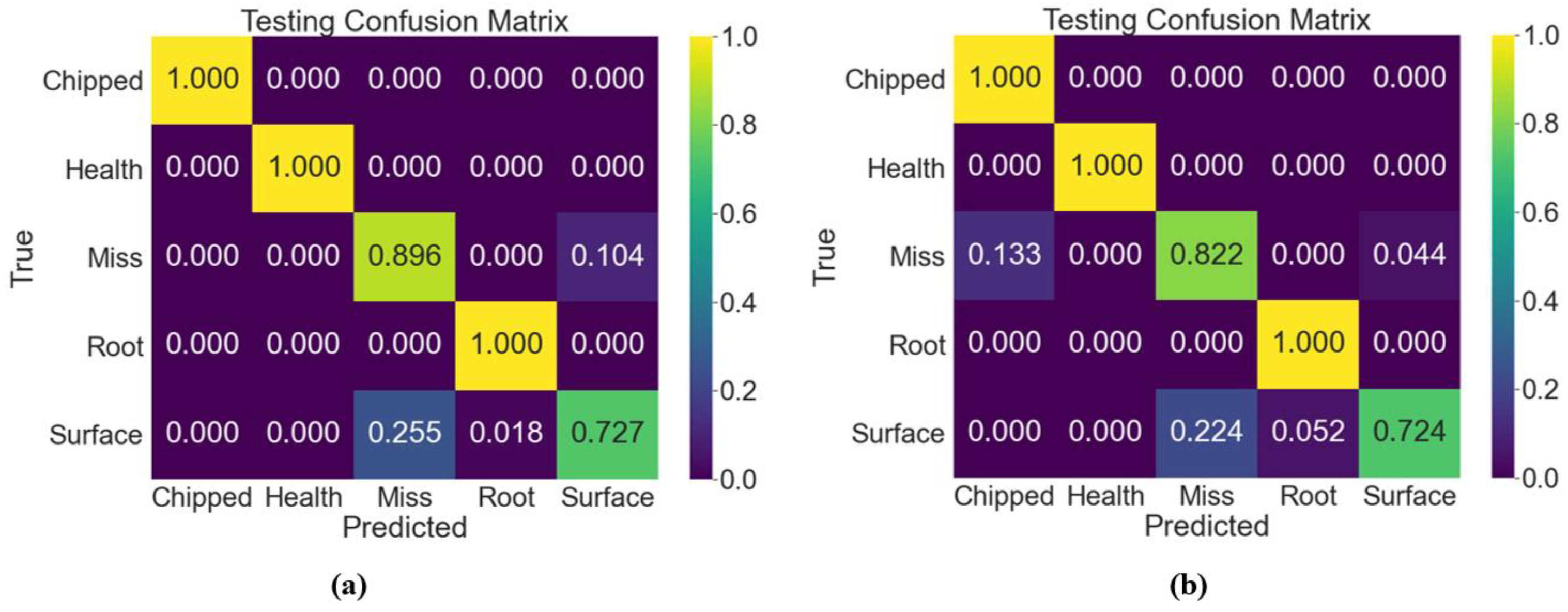
4.3. Additional Dataset Validation

In addition to Southeast University experimental dataset introduced above, to further validate the proposed method, we also used the experimental data collected by the GDS3000 (SpectraQuest, Inc., Richmond, VA, USA) experimental platform. The platform is equipped with switchable normal bearings, inner fault bearings, outer fault bearings, rolling-element fault bearings, and compound fault bearings (with inner and outer fault), as shown in Figure 14.

Using the GDS3000 experimental platform, data were collected based on two working conditions: medium–high speed (1540 r/min) and high speed (1788 r/min). The experimental results in

Table 7. Results of GDS 3000 experimental platform.

Operation Conditions	Medium–High Speed (1540 r/min)				High Speed (1788 r/min)
Model	SVM	KNN	RF	GBDT	SVM	KNN	RF	GBDT
VMD energy entropy	98.40%	98.53%	98.53%	97.44%	98.53%	98.53%	98.17%	97.44%
SVMD energy entropy	98.17%	95.60%	95.24%	94.14%	94.46%	97.42%	94.46%	94.10%
VMD fuzzy entropy	94.56%	98.40%	98.53%	98.17%	96.70%	98.90%	91.58%	95.97%
SVMD fuzzy entropy	97.07%	98.53%	95.97%	96.34%	96.31%	97.42%	95.94%	94.84%

show that the fuzzy entropy was superior to the energy entropy.

5. Discussion and Open Issues

5.1. Classification-Model Design

In this paper, we used four classification models: SVM, KNN, RF, and GBDT.

Table 8. Comparison of classification models.

Model	Applicable Data	Classification Problem	Training Time	Storage Space
SVM	Low-dimensional	Linear classification	Long	Low
KNN	Low-dimensional	Nonlinear classification	Short	High
RF	High-dimensional	Nonlinear classification	Long	Low
GBDT	High-dimensional	Nonlinear classification	Long	Low

shows the comparison of the classification models for reference. However, in practical industrial applications, the design of a classification method requires the consideration of several factors, including the type of data, the type of classification problem, the size of the data set and the number of features, the accuracy requirements, the interpretability, and the complexity of the model. When designing a model, these factors need to be considered comprehensively, and the most appropriate model should be selected based on practical applications.

5.2. Research Limitations

In terms of the limitations of our research, we agree that further optimization of the classification-model parameters is needed to improve accuracy. Additionally, our study focused on a limited dataset, and more industrial data are needed to validate the model’s performance in real-world applications.

As for future research directions, we plan to explore more advanced optimization techniques to further improve the accuracy of the classification model. We also plan to collect more diverse and comprehensive industrial data to better validate the model’s performance in various industrial applications. In addition, we plan to investigate the potential of incorporating other datasets to further enhance the model’s accuracy. We believe that these future research directions will contribute to the development of more robust and accurate models for industrial applications.

6. Conclusions

An effective signal-decomposition method is an important tool for mechanical-fault diagnosis. The original vibration signal contains a lot of information. By decomposing the original signal into individual components and analyzing each of them, it is easy to find the faults present in the machine. This paper used an iterative SVMD method that decomposes the signal into its constituent components, which is a successive implementation of VMD. It can also be seen as an extension of the VME method. This method was built by adding some criteria to the VMD algorithm to distinguish it from the previous one. The advantage of SVMD over VMD is that it does not need to know the number of modes available in the signal and converges to almost the same mode pattern as VMD with a known number of modes k. The performance was even better than VMD in some cases.

The energy entropy and fuzzy entropy of each component were obtained by decomposing the vibration signals under two working conditions of SEU gears by VMD and SVMD. Each of them was constructed into the energy-entropy sample sets and fuzzy-entropy sample sets, which were trained and tested in the established machine-learning classification models SVM, k-NN, RF, and GBDT. The results show that in SEU gearbox working condition I, the SVMD energy entropy, the fuzzy entropy in SVM and k-NN models, and the classification accuracy of VMD energy entropy were above 90%. The classification accuracy of the VMD energy entropy was poor. Whereas in integrated learning, the classification accuracy of VMD and SVMD fuzzy entropy and energy entropy were not much different, in SEU gearbox case II, the classification accuracy of SVMD energy entropy and fuzzy entropy was the highest in SVM and k-NN classification. The accuracy was close to 90%. The classification accuracy of VMD was even worse compared with SVMD. The same phenomenon occurred in integrated learning, as well.

Finally, the SVMD feature-extraction diagnosis results of this paper for the gearbox data of SEU were compared with the results of other literature The overall effect was better than the results of the method in the literature, which verifies the effectiveness of the SVMD feature-extraction method.

References

1. Trizoglou, P.; Liu, X.; Lin, Z. Fault detection by an ensemble framework of Extreme Gradient Boosting (XGBoost) in the operation of offshore wind turbines. Renew. Energy 2021, 179, 945–962. [Google Scholar] [CrossRef]
2. Liu, J.; Yang, G.; Li, X.; Hao, S.; Guan, Y.; Li, Y. A deep generative model based on CNN-CVAE for wind turbine condition monitoring. Meas. Sci. Technol. 2023, 34, 035902. [Google Scholar] [CrossRef]
3. Zhao, H.; Yang, X.; Chen, B.; Chen, H.; Deng, W. Bearing fault diagnosis using transfer learning and optimized deep belief network. Meas. Sci. Technol. 2022, 33, 065009. [Google Scholar] [CrossRef]
4. Xie, T.; Xu, Q.; Jiang, C.; Lu, S.; Wang, X. The fault frequency priors fusion deep learning framework with application to fault diagnosis of offshore wind turbines. Renew. Energy 2023, 202, 143–153. [Google Scholar] [CrossRef]
5. Vukelic, G.; Pastorcic, D.; Vitzentin, G.; Bozic, Z. Failure investigation of a crane gear damage. Eng. Fail. Anal. 2020, 115, 104613. [Google Scholar] [CrossRef]
6. Yang, F.; Huang, D.; Li, D.; Zhao, Y.; Lin, S.; Muyeen, S.M. A novel convolutional network with a self-adaptation high-pass filter for fault diagnosis of wind turbine gearboxes. Meas. Sci. Technol. 2023, 34, 025024. [Google Scholar] [CrossRef]
7. Das, S.; Prusty, B.R.; Bingi, K. Review of adaptive decomposition-based data preprocessing for renewable generation rich power system applications. J. Renew. Sustain. Energy 2021, 13, 062703. [Google Scholar] [CrossRef]
8. Yu, K.; Lin, T.R.; Tan, J.; Ma, H. An adaptive sensitive frequency band selection method for empirical wavelet transform and its application in bearing fault diagnosis. Measurement 2019, 134, 375–384. [Google Scholar] [CrossRef]
9. Liu, X.; Zhu, A.; Song, Y.; Ma, G.; Bai, X.; Guo, Y. Application of Improved Robust Local Mean Decomposition and Multiple Disturbance Multi-Verse Optimizer-Based MCKD in the Diagnosis of Multiple Rolling Element Bearing Faults. Machines 2022, 10, 883. [Google Scholar] [CrossRef]
10. Babu, T.N.; Devendiran, S.; Aravind, A.; Rakesh, A.; Jahzan, M. Fault Diagnosis on Journal Bearing Using Empirical Mode Decomposition. Mater. Today-Proc. 2018, 5, 12993–13002. [Google Scholar] [CrossRef]
11. Vamsi, I.; Sabareesh, G.R.; Vaibhav, S. Integrated Vibro-Acoustic Analysis and Empirical Mode Decomposition for Fault Diagnosis of Gears in a Wind Turbine. Procedia Struct. Integr. 2019, 14, 937–944. [Google Scholar]
12. Xiong, J.; Chen, K.; Cen, J.; Wang, Q.; Liu, X. Application of multi-kernel relevance vector machine and data pre-processing by complementary ensemble empirical mode decomposition and mutual dimensionless in fault diagnosis. Meas. Sci. Technol. 2022, 33, 115018. [Google Scholar] [CrossRef]
13. Hoseinzadeh, M.S.; Khadem, S.E.; Sadooghi, M.S. Quantitative diagnosis for bearing faults by improving ensemble empirical mode decomposition. ISA Trans. 2018, 83, 261–275. [Google Scholar] [CrossRef]
14. Sahu, P.K.; Rain, R.N. Fault Diagnosis of Rolling Bearing Based on an Improved Denoising Technique Using Complete Ensemble Empirical Mode Decomposition and Adaptive Thresholding Method. J. Vib. Eng. Technol. 2023, 11, 513–535. [Google Scholar] [CrossRef]
15. Cheng, Y.; Wang, Z.; Chen, B.; Zhang, W.; Huang, G. An improved complementary ensemble empirical mode decomposition with adaptive noise and its application to rolling element bearing fault diagnosis. ISA Trans. 2019, 91, 218–234. [Google Scholar] [CrossRef]
16. Wang, L.M.; Shao, Y.M. Fault feature extraction of rotating machinery using a reweighted complete ensemble empirical mode decomposition with adaptive noise and demodulation analysis. Mech. Syst. Signal Process. 2020, 138, 106545. [Google Scholar] [CrossRef]
17. Ma, J.; Zhuo, S.; Li, C.; Zhan, L.; Zhang, G. An Enhanced Intrinsic Time-Scale Decomposition Method Based on Adaptive Levy Noise and Its Application in Bearing Fault Diagnosis. Symmetry 2021, 13, 617. [Google Scholar] [CrossRef]
18. Pazoki, M.; Chaitanya, B.K.; Yadav, A. A new wave-based fault detection scheme during power swing. Electr. Power Syst. Res. 2023, 246, 109077. [Google Scholar] [CrossRef]
19. Dragomiretskiy, K.; Zosso, D. Variational Mode Decomposition. IEEE Trans. Signal Process. 2014, 62, 531–544. [Google Scholar] [CrossRef]
20. Li, Y.; Cheng, G.; Liu, C.; Chen, X. Study on planetary gear fault diagnosis based on variational mode decomposition and deep neural networks. Measurement 2018, 130, 94–104. [Google Scholar] [CrossRef]
21. Zhang, J.; Wu, J.; Hu, B.; Tang, J. Intelligent fault diagnosis of rolling bearings using variational mode decomposition and self-organizing feature map. J. Vib. Control 2020, 26, 1886–1897. [Google Scholar] [CrossRef]
22. Liu, W.; Liu, Y.; Li, S.; Chen, Y. A Review of Variational Mode Decomposition in Seismic Data Analysis. Surv. Geophys. 2022, 44, 323–355. [Google Scholar] [CrossRef]
23. Li, C.; Liu, Y.; Liao, Y. An Improved Parameter-Adaptive Variational Mode Decomposition Method and Its Application in Fault Diagnosis of Rolling Bearings. Shock Vib. 2021, 2021, 2969488. [Google Scholar] [CrossRef]
24. Gai, J.; Shen, J.; Hu, Y.; Wang, H. An integrated method based on hybrid grey wolf optimizer improved variational mode decomposition and deep neural network for fault diagnosis of rolling bearing. Measurement 2020, 162, 107901. [Google Scholar] [CrossRef]
25. Yan, X.; Jia, M. Bearing fault diagnosis via a parameter-optimized feature mode decomposition. Measurement 2022, 203, 112016. [Google Scholar] [CrossRef]
26. Nguyen, C.D.; Ahmad, Z.; Kim, J.-M. Gearbox Fault Identification Framework Based on Novel Localized Adaptive Denoising Technique, Wavelet-Based Vibration Imaging, and Deep Convolutional Neural Network. Appl. Sci. 2021, 11, 7575. [Google Scholar] [CrossRef]
27. Ahmad, Z.; Nguyen, T.-K.; Ahmad, S.; Nguyen, C.D.; Kim, J.-M. Multistage Centrifugal Pump Fault Diagnosis Using Informative Ratio Principal Component Analysis. Sensors 2022, 22, 179. [Google Scholar] [CrossRef]
28. Nazari, M.; Sakhaei, S.M. Successive variational mode decomposition. Signal Process. 2020, 174, 107610. [Google Scholar] [CrossRef]
29. Nazari, M.; Sakhaei, S.M. Variational Mode Extraction: A New Efficient Method to Derive Respiratory Signals from ECG. IEEE J. Biomed. Health Inform. 2018, 22, 1059–1067. [Google Scholar] [CrossRef]
30. Chen, X.; Yang, Y.; Cui, Z.; Shen, J. Vibration fault diagnosis of wind turbines based on variational mode decomposition and energy entropy. Energy 2019, 174, 1100–1109. [Google Scholar] [CrossRef]
31. Jiao, J.; Yue, J.; Pei, D. Feature Enhancement Method of Rolling Bearing Based on K-Adaptive VMD and RBF-Fuzzy Entropy. Entropy 2022, 24, 197. [Google Scholar] [CrossRef] [PubMed]
32. Shao, S.; McAleer, S.; Yan, R.; Baldi, P. Highly Accurate Machine Fault Diagnosis Using Deep Transfer Learning. IEEE Trans. Ind. Inform. 2019, 15, 2446–2455. [Google Scholar] [CrossRef]
33. Lei, Y.; Yang, B.; Jiang, X.; Jia, F.; Li, N.; Nandi, A.K. Applications of machine learning to machine fault diagnosis: A review and roadmap. Mech. Syst. Signal Process. 2020, 138, 106587. [Google Scholar] [CrossRef]
34. Cui, M.; Wang, Y.; Lin, X.; Zhong, M. Fault Diagnosis of Rolling Bearings Based on an Improved Stack Autoencoder and Support Vector Machine. IEEE Sens. J. 2021, 21, 4927–4937. [Google Scholar] [CrossRef]
35. Yu, T.; Chen, X.; Yan, W.; Xu, Z.; Ye, M. Leak detection in water distribution systems by classifying vibration signals. Mech. Syst. Signal Process. 2023, 185, 109810. [Google Scholar] [CrossRef]
36. Albaqami, H.; Hassan, G.M.; Subasi, A.; Datta, A. Automatic detection of abnormal EEG signals using wavelet feature extraction and gradient boosting decision tree. Biomed. Signal Process. Control 2021, 70, 102957. [Google Scholar] [CrossRef]
37. Hosseinpour-Zarnaq, M.; Omid, M.; Biabani-Aghdam, E. Fault diagnosis of tractor auxiliary gearbox using vibration analysis and random forest classifier. Inf. Process. Agric. 2022, 9, 60–67. [Google Scholar] [CrossRef]
38. Zhao, R.; Wang, D.; Yan, R.; Mao, K.; Shen, F.; Wang, J. Machine Health Monitoring Using Local Feature-Based Gated Recurrent Unit Networks. IEEE Trans. Ind. Electron. 2018, 65, 1539–1548. [Google Scholar] [CrossRef]
Figure 1. Time-domain–frequency-domain diagram of the simulated signal: (a) signal time-domain waveform; (b) signal frequency-domain diagram.
Algorithms 16 00304 g001
Figure 2. VMD signal-decomposition-component time-domain–frequency-domain diagram: (a) time-domain diagram of each component; (b) frequency-domain diagram of each component.
Algorithms 16 00304 g002
Figure 3. SVMD signal-decomposition-component time-domain–frequency-domain diagram: (a) time-domain diagram of each component; (b) frequency-domain diagram of each component.
Algorithms 16 00304 g003
Figure 4. Time-domain–frequency-domain diagram of the simulated signal with superimposed random signal: (a) time-domain diagram of the random signal; (b) X t signal time-domain frequency-domain diagram.
Algorithms 16 00304 g004
Figure 5. VMD signal-decomposition-component time-domain–frequency-domain diagram: (a) time-domain diagram of each component; (b) frequency-domain diagram of each component.
Algorithms 16 00304 g005
Figure 6. SVMD signal-decomposition-component time-domain–frequency-domain plots: (a) time-domain plots of each component; (b) frequency-domain plots of each component.
Algorithms 16 00304 g006
Figure 7. Simulated signal-component energy entropy: (a) component energy entropy of x t ; (b) component energy entropy of X t .
Algorithms 16 00304 g007
Figure 8. Correlation-confusion matrix of x t : (a) VMD decomposition correlation of x t ; (b) SVMD decomposition correlation of x t .
Algorithms 16 00304 g008
Figure 9. Correlation-confusion matrix of X(t): (a) VMD decomposition correlation of X(t); (b) SVMD decomposition correlation of X(t).
Algorithms 16 00304 g009
Figure 10. Simulated signal-component fuzzy entropy: (a) component fuzzy entropy of x(t); (b) component fuzzy entropy of X(t).
Algorithms 16 00304 g010
Figure 11. Experimental flowchart.
Algorithms 16 00304 g011
Figure 12. Confusion matrix of SVM classification of gearbox working condition I energy entropy in the SEU dataset: (a) VMD; (b) SVMD.
Algorithms 16 00304 g012
Figure 13. Confusion matrix of fuzzy-entropy SVM classification of gearbox working condition I in the SEU dataset: (a) VMD; (b) SVMD.
Algorithms 16 00304 g013
Figure 14. GDS3000 experimental platform.
Algorithms 16 00304 g014